The numerical computation of unstable manifolds for infinite dimensional dynamical systems by embedding techniques

Abstract.

In this work we extend the novel framework developed in [9] to the computation of finite dimensional unstable manifolds of infinite dimensional dynamical systems. To this end, we adapt a set-oriented continuation technique developed in [10] for the computation of such objects of finite dimensional systems with the results obtained in [9]. We show how to implement this approach for the analysis of partial differential equations and illustrate its feasibility by computing unstable manifolds of the one-dimensional Kuramoto-Sivashinsky equation as well as for the Mackey-Glass delay differential equation.

Adrian Ziessler, Michael Dellnitz and Raphael Gerlach

Department of Mathematics

Paderborn University

33095 Paderborn, Germany

1. Introduction

Set-oriented numerical methods have been developed in the context of the numerical treatment of dynamical systems (e. g. [11, 12, 16, 18]). The basic idea of these methods is to cover the objects of interest – for instance invariant sets or global attractors – by outer approximations which are created via multilevel subdivision or continuation techniques. They have been used in several different application areas such as molecular dynamics ([42]), astrodynamics ([13]) or ocean dynamics ([17]).

The computation of (global) invariant manifolds has attracted a lot of interest in recent years. Approaches based on geometric concepts can be used to approximate (up to two-dimensional) unstable manifolds of vector fields (see [33] for an overview). The approximation by geodesic level sets, for instance, produces a regular mesh that consists of geodesic circles by solving appropriate boundary value problems (e.g., [31, 32]). Topological methods are used to create outer approximations of invariant manifolds. In [33] a survey of different approaches for computing global stable or unstable manifolds of vector fields is given.

In this paper, we will focus on the set-oriented continuation method that has been developed in [10] and we will show how to use it for the computation of unstable manifolds of infinite dimensional dynamical systems. We will, in particular, approximate unstable manifolds for semiflows of Banach spaces (cf. [20, 22, 3, 5]). Our approach relies on the results obtained in [9], where the subdivision technique developed in [11] has been extended to the infinite dimensional context. The underlying idea is to compute low dimensional invariant sets of infinite dimensional dynamical systems by utilizing embedding techniques for infinite dimensional systems [24, 40]. To this end, a delay embedding technique has been used in order to obtain a one-to-one representation of the (infinite dimensional) dynamics by the so-called core dynamical system (CDS). The CDS is a continuous dynamical system on a state space of moderate dimension which we will refer to as the observation space. Then the subdivision scheme from [11] has been applied to the CDS in order to analyze one-to-one images of global attractors for the infinite dimensional dynamical system. The feasibility of this approach has been illustrated by computing invariant sets for delay differential equations with constant time delay. Recently, this approach has also been generalized to delay differential equations with state dependent time delay [47]. In [2] low-dimensional transition manifolds of stochastic dynamical systems showing metastable behavior have been parameterized by using a combination of embedding and manifold learning techniques.

In addition to delay differential equations, other application scenarios in which finite dimensional invariant sets arise are certain types of dissipative dynamical systems described by partial differential equations, for instance the Kuramoto-Sivashinsky equation [34, 44], the Ginzburg-Landau equation, or scalar reaction-diffusion equations with cubic nonlinearity [27]. For all these systems a finite dimensional so-called inertial manifold exists to which trajectories are attracted exponentially fast, e.g., [7, 15, 45].

In this paper we extend the classical set-oriented continuation technique developed in [10] to the infinite dimensional context. This method allows us to approximate unstable manifolds of infinite dimensional dynamical systems in observation space. The general numerical approach we are proposing is in principle applicable to infinite dimensional dynamical systems described by a Lipschitz continuous operator on a Banach space. However, in this article we will focus on partial differential equations (PDEs). To this end, we will develop an appropriate numerical realization of the CDS for PDEs and illustrate the efficiency of our method for a one-dimensional Kuramoto-Sivashinsky equation. The Kuramoto-Sivashinsky equation has attracted a lot of interest as a model for complex spatio-temporal dynamics and has been derived in the context of several extended physical problems, e.g., phase dynamics in reaction-diffusion systems [34] or small thermal diffusive instabilities in laminar flame fronts [44]. It is also a paradigm for the existence of complex finite dimensional dynamics in a PDE. In addition, we will also illustrate the efficiency of our method for the Mackey-Glass delay differential equation by using the numerical realization of the CDS introduced in [9]. In the context of delay differential equations a related – though not set-oriented – approach has recently been utilized in [19] for the numerical approximation of unstable manifolds. In this work the authors compute high order Taylor and Fourier-Taylor approximations of unstable manifolds for equilibria or periodic solutions.

A detailed outline of the paper is as follows. In Section 2 we briefly summarize the results of [9]. We state the main results of [24] and [40] and we describe the construction of the CDS on the observation space. In Section 3 we first briefly review the continuation method developed in [10] for the computation of unstable manifolds of finite dimensional dynamical systems. Then we explain how to use this technique in the context of infinite dimensional dynamical systems. In [10] convergence has been shown for compact subsets of unstable manifolds. Here we will extend this convergence result to the closure of the entire unstable manifold. In particular, we will prove that in this setting the embedding of the local unstable manifold (in infinite dimensional space) is identical to the local embedded unstable manifold (cf. Proposition 4 (b)). A numerical realization for the construction of the CDS for PDEs is given in Section 4. Finally, in Section 5, we illustrate the efficiency of our method for the Mackey-Glass delay differential equation and for a one-dimensional Kuramoto-Sivashinsky equation. We will, in particular, generate numerical approximations of one-to-one copies of unstable manifolds for the Kuramoto-Sivashinsky equation for different parameter values.

2. Review of subdivision and embedding results

Since our set-oriented continuation method is based on the framework developed in [9] we start with a short review of the related material.

2.1. Basic definitions and results from embedding theory

We consider dynamical systems of the form

$$u_{j+1}=\Phi(u_{j}),\quad j=0,1,\ldots,$$ (1)

where $\Phi:Y\rightarrow Y$ is Lipschitz continuous on a Banach space $Y$. Moreover we assume that $\Phi$ has an invariant compact set $\mathcal{A}$, that is

$$\Phi(\mathcal{A})=\mathcal{A}.$$

This assumption is justified by several classical results, where it has been shown that for many dissipative systems on Banach spaces there exist (non-trivial) compact attractors of finite capacity or Hausdorff dimension (see [38, 36, 8, 6, 21]). In order to approximate the set $\mathcal{A}$ we combine a classical subdivision technique for the computation of such objects in a finite dimensional space with infinite dimensional embedding results (cf. [24, 40]). For the statement of the main result of [40] we need three particular notions: prevalence [41], upper box counting dimension and thickness exponent [24].

Definition 2.1.

1. A Borel subset $S$ of a normed linear space $V$ is prevalent if there is a finite dimensional subspace $E$ of $V$ (the ‘probe space’) such that for each $v\in V,\ v+e$ belongs to $S$ for (Lebesgue) almost every $e\in E$.

2. Let $Y$ be a Banach space, and let $\mathcal{A}\subset Y$ be compact. For $\varepsilon>0$, denote by $N_{Y}(\mathcal{A},\varepsilon)$ the minimal number of balls of radius $\varepsilon$ (in the norm of $Y$) necessary to cover the set $\mathcal{A}$. Then

   $$d(\mathcal{A};Y)=\limsup\limits_{\varepsilon\rightarrow 0}\frac{\log N_{Y}(\mathcal{A},\varepsilon)}{-\log\varepsilon}=\limsup_{\varepsilon\to 0}\;-\log_{{\varepsilon}}N_{Y}(\mathcal{A},\varepsilon)$$

   denotes the upper box-counting dimension of $\mathcal{A}$.

3. Let $Y$ be a Banach space, and let $\mathcal{A}\subset Y$ be compact. For $\varepsilon>0$, denote by $d_{Y}(\mathcal{A},\varepsilon)$ the minimal dimension of all finite dimensional subspaces $V\subset Y$ such that every point of $\mathcal{A}$ lies within distance $\varepsilon$ of $V$; if no such $V$ exists, $d_{Y}(\mathcal{A},\varepsilon)=\infty$. Then

   $$\sigma(\mathcal{A},Y)=\limsup_{\varepsilon\to 0}\;-\log_{{\varepsilon}}d_{Y}(\mathcal{A},\varepsilon)$$

   is called the thickness exponent of $\mathcal{A}$ in $Y$.

With these definitions the main results relevant for our framework are as follows:

Theorem 2.2 ([24]).

Let $Y$ be a Banach space and $\mathcal{A}\subset Y$ compact, with upper box counting dimension $d=d(\mathcal{A};Y)$ and thickness exponent $\sigma=\sigma(\mathcal{A},Y)$. Let $N>2d$ be an integer, and let $\alpha\in\mathbb{R}$ with

$$0<\alpha<\frac{N-2d}{N\cdot(1+\sigma)}.$$

Then for a prevalent set of bounded linear maps $\mathcal{L}:Y\to\mathbb{R}^{N}$ there is $C>0$ such that

$$C\cdot\|\mathcal{L}(x-y)\|^{\alpha}\geq\|x-y\|\quad\text{for all }x,y\in\mathcal{A}.$$

Note that this result implies that – if $N$ is large enough – a prevalent set of bounded linear maps ${\mathcal{L}:Y\to\mathbb{R}^{N}}$ will be one-to-one on $\mathcal{A}$. This theorem lays the foundation for Robinson’s main result concerning delay embedding techniques:

Theorem 2.3 ([40]).

Let $Y$ be a Banach space and $\mathcal{A}\subset Y$ a compact, invariant set, with upper box counting dimension $d$, and thickness exponent $\sigma$. Choose an integer $k>2(1+\sigma)d$ and suppose further that the set $\mathcal{A}_{p}$ of $p$-periodic points of $\Phi$ satisfies $d(\mathcal{A}_{p};Y)<p/(2+2\sigma)$ for $p=1,\ldots,k$. Then for a prevalent set of Lipschitz maps $f:Y\rightarrow\mathbb{R}$ the observation map $D_{k}[f,\Phi]:Y\rightarrow\mathbb{R}^{k}$ defined by

$$D_{k}[f,\Phi](u)=\left(f(u),f(\Phi(u)),\ldots,f(\Phi^{k-1}(u))\right)^{T}$$ (2)

is one-to-one on $\mathcal{A}$.

Remark 1.

1. This result can be generalized to the case where several different observables are evaluated. More precisely, for a prevalent set of Lipschitz maps ${f_{i}:Y\to\mathbb{R}}$, $i=1,\dots,q\leq k$, the observation map ${D_{k}[f_{1},\ldots,f_{q},\Phi]:Y\to\mathbb{R}^{k}}$,

   $$u\mapsto\left(f_{1}(u),\ldots,f_{1}\left(\Phi^{k_{1}-1}(u)\right),\ldots,f_{q}(u),\ldots,f_{q}\left(\Phi^{k_{q}-1}(u)\right)\right)^{T}$$

   is also one-to-one on $\mathcal{A}$, provided that

   $$k=\sum_{i=1}^{q}k_{i}>2(1+\sigma)\cdot d\ \mbox{ and }\ {d(\mathcal{A}_{p})<p/(2+2\sigma)}\quad\forall p\leq\max(k_{1},\ldots,k_{q}).$$

2. As observed in [24], the thickness exponent is always bounded by the (upper) box-counting dimension, i.e.,

   $$\sigma(\mathcal{A},Y)\leq d(\mathcal{A};Y).$$

   Thus, providing that we know the upper box-counting dimension $d$ of $\mathcal{A}$ we can in principle always choose a worst-case embedding dimension $k$ such that

   $$k>2(1+d)d$$

   is satisfied (cf. Theorem 2.3).

2.2. The core dynamical system (CDS)

In [9] the results from Section 2.1 have been used to create a finite dimensional dynamical system that allows to approximate invariant sets for infinite dimensional dynamical systems on Banach spaces. In this section we will briefly review the construction of the CDS.

Let $\mathcal{A}$ be a compact invariant set of the infinite dimensional dynamical system (1). We denote by $A_{k}$ the image of $\mathcal{A}\subset Y$ under the observation map $R:Y\rightarrow\mathbb{R}^{k}$, that is

$$A_{k}=R(\mathcal{A}),$$ (3)

where $R=\mathcal{L}$ according to Theorem 2.2 or $R=D_{k}[f,\Phi]$ according to Theorem 2.3. We then construct the CDS

$$x_{j+1}=\varphi(x_{j}),\quad j=0,1,2,\ldots,$$ (4)

with $\varphi:\mathbb{R}^{k}\rightarrow\mathbb{R}^{k}$ as follows: At first we define $\varphi$ on the set $A_{k}$ by

$$\varphi=R\circ\Phi\circ\widetilde{E},$$

where $\widetilde{E}:A_{k}\rightarrow Y$ is the continuous map satisfying

$$(\widetilde{E}\circ R)(u)=u\quad\forall u\in\mathcal{A}\quad\text{ and }\quad(R\circ\widetilde{E})(x)=x\quad\forall x\in A_{k}.$$ (5)

In fact, this is possible since $R$ is invertible as a mapping from $\mathcal{A}$ to $A_{k}$. Observe that by this construction $A_{k}$ is an invariant set for $\varphi$. By using a generalization of Tietze’s extension theorem by Dugundji [14] we extend $\widetilde{E}$ to a continuous map $E:\mathbb{R}^{k}\to Y$ with $E_{|A_{k}}=\widetilde{E}$ (see Fig. 1).

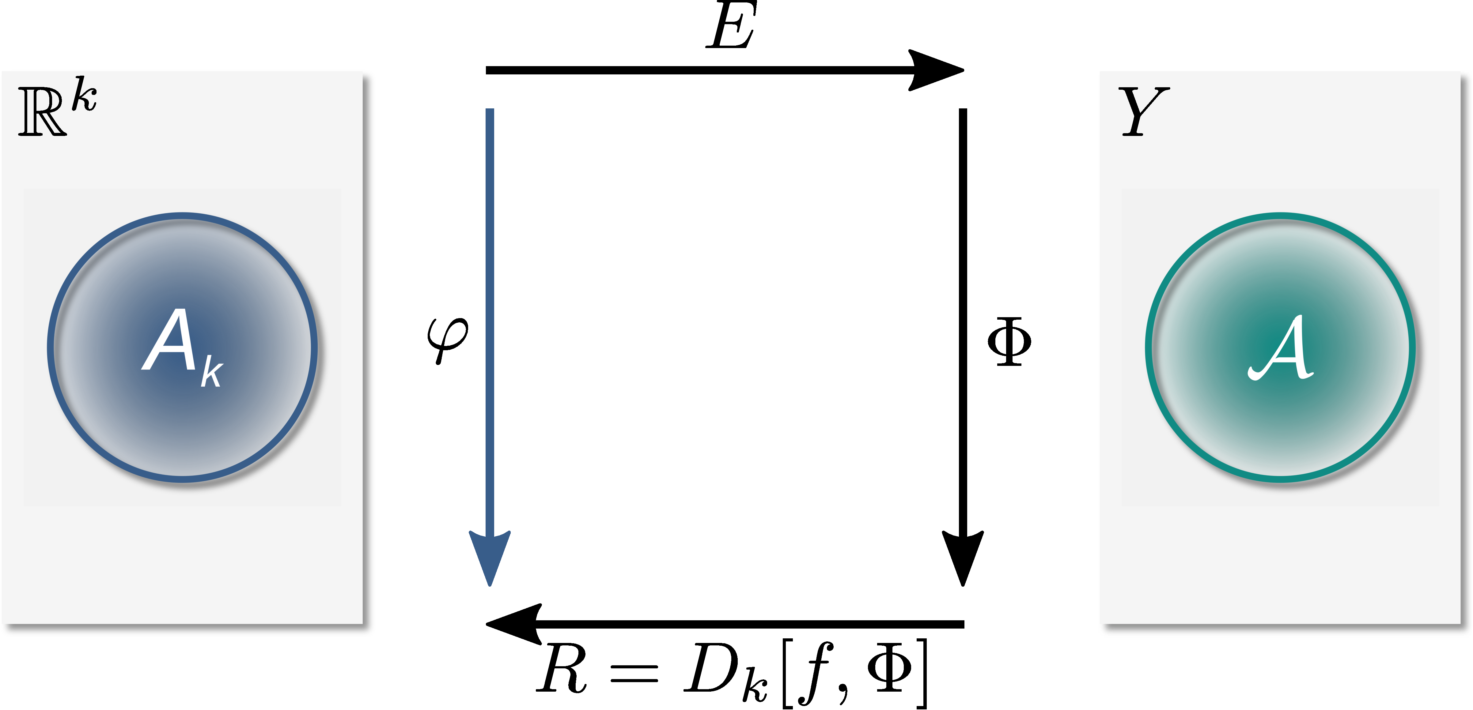
Figure 1. Definition of the CDS $\varphi$.

Now we are in the position to extend the CDS $\varphi$ to $\mathbb{R}^{k}$:

Proposition 1.

There is a continuous map $\varphi:\mathbb{R}^{k}\to\mathbb{R}^{k}$ satisfying

$$\varphi(R(u))=R(\Phi(u))\text{ for all }u\in\mathcal{A}.$$

For the proof the reader is referred to [9].

2.3. Computation of embedded attractors via subdivision

By our construction, the dynamics of the CDS $\varphi$ on $A_{k}$ is topologically conjugate to that of $\Phi$ on $\mathcal{A}$. In what follows we will briefly review the main statements of [9]. We will use (4) in order to approximate the embedded invariant set $A_{k}$ (cf. (3)) via subdivision. To this end, we give a brief review of the related subdivision scheme.

Subdivision scheme: Let $Q\subset\mathbb{R}^{k}$ be a compact set. We define the global attractor relative to $Q$ by

$$A_{Q}=\bigcap_{j\geq 0}\varphi^{j}(Q).$$ (6)

The aim is to approximate this set with the subdivision procedure. By using the subdivision algorithm we obtain a sequence ${\mathcal{B}}_{0},{\mathcal{B}}_{1},\ldots$ of finite collections of compact subsets of $\mathbb{R}^{k}$ such that the diameter

$$\mathop{\rm diam}\nolimits({\mathcal{B}}_{\ell})=\max_{B\in{\mathcal{B}}_{\ell}}\mathop{\rm diam}\nolimits(B)$$

converges to zero for $\ell\rightarrow\infty$. Given an initial collection ${\mathcal{B}}_{0}$, we inductively obtain ${\mathcal{B}}_{\ell}$ from ${\mathcal{B}}_{\ell-1}$ for $\ell=1,2,\ldots$ in two steps.

1. Subdivision: Construct a new collection $\hat{\mathcal{B}}_{\ell}$ such that

   $$\bigcup_{B\in\hat{\mathcal{B}}_{\ell}}B=\bigcup_{B\in{\mathcal{B}}_{\ell-1}}B$$ (7)

   and

   $$\mathop{\rm diam}\nolimits(\hat{\mathcal{B}}_{\ell})=\theta_{\ell}\mathop{\rm diam}\nolimits({\mathcal{B}}_{\ell-1}),$$ (8)

   where $0<\theta_{\min}\leq\theta_{\ell}\leq\theta_{\max}<1$.

2. Selection: Define the new collection ${\mathcal{B}}_{\ell}$ by

   $${\mathcal{B}}_{\ell}=\left\{B\in\hat{\mathcal{B}}_{\ell}:\exists\hat{B}\in\hat{\mathcal{B}}_{\ell}\leavevmode\nobreak\ \mbox{such that}\leavevmode\nobreak\ \varphi^{-1}(B)\cap\hat{B}\neq\emptyset\right\}.$$ (9)

The first step guarantees that the collections ${\mathcal{B}}_{\ell}$ contains successively finer sets for increasing $\ell$. In fact, by construction

$$\mathop{\rm diam}\nolimits({\mathcal{B}}_{\ell})\leq\theta_{\max}^{\ell}\mathop{\rm diam}\nolimits({\mathcal{B}}_{0})\rightarrow 0\quad\mbox{for $\ell\rightarrow\infty$.}$$ (10)

In the second step we remove each subset whose preimage does neither intersect itself nor any other subset in $\hat{\mathcal{B}}_{\ell}$.

Denote by $Q_{\ell}$ the collection of compact subsets obtained after $\ell$ subdivision steps, that is

$$Q_{\ell}=\bigcup_{B\in{\mathcal{B}}_{\ell}}B.$$

Observe that the $Q_{\ell}$’s define a nested sequence of compact sets, that is, $Q_{\ell+1}\subset Q_{\ell}$. Therefore, for each $m$,

$$Q_{m}=\bigcap\limits_{\ell=1}^{m}Q_{\ell},$$ (11)

and we may view

$$Q_{\infty}=\bigcap\limits_{\ell=1}^{\infty}Q_{\ell}$$ (12)

as the limit of the $Q_{\ell}$’s. Then the selection step is responsible for the fact that the unions $Q_{\ell}$ approach the relative global attractor:

Proposition 2.

Suppose that $A_{Q}$ satisfies $\varphi^{-1}(A_{Q})\subset A_{Q}$. Then

$$A_{Q}=Q_{\infty}.$$

Observe that in contrast to [11] we have to assume that $\varphi^{-1}(A_{Q})\subset A_{Q}$ since the CDS is only continuous and not homeomorphic. Moreover, we note that we can, in general, not expect that $A_{k}=A_{Q}$. In fact, by construction $A_{Q}$ may contain several invariant sets and related heteroclinic connections. However, if $\mathcal{A}$ is an attracting set we can prove equality:

Proposition 3.

1. Let $A_{Q}$ be the global attractor relative to the compact set $Q$, and suppose that the embedded attractor $A_{k}$ satisfies $A_{k}\subset Q$. Then

   $$A_{k}\subset A_{Q}.$$ (13)

2. Suppose that $\mathcal{A}$ is an attracting set with basin of attraction $\mathcal{U}\supset\mathcal{A}$ and choose $Q\subset\mathbb{R}^{k}$ such that $A_{k}\subset Q$ and $E(Q)\subset\mathcal{U}$. Define for $m\geq 1$ the continuous maps

   $$\varphi_{m}=R\circ\Phi^{m}\circ E$$

   and denote the corresponding relative global attractors by $A_{Q}^{m}$, where

   $$A_{Q}^{m}=\bigcap_{j\geq 0}\varphi_{m}^{j}(Q).$$

   Then

   $$A_{k}=A_{Q}^{\infty},$$

   where $A_{Q}^{\infty}=\bigcap_{m\geq 1}A_{Q}^{m}$.

Remark 2.

Roughly speaking Proposition 3 (b) states that it is possible to approximate an attracting set for $\Phi$ if we perform the computations with appropriately high iterates of $\Phi$.

3. A subdivision and continuation technique for embedded unstable manifolds

In this section we extend the results of [10] for the computation of finite dimensional unstable manifolds of infinite dimensional dynamical systems of the form (1). We will in particular focus on invariant manifolds for semiflows on Banach spaces (cf. [20, 22, 3, 5]).

3.1. Approximation of the local unstable manifold

Let us denote by

$${\mathcal{W}}_{\Phi}^{u}(u^{*})\subset\mathcal{A}$$ (14)

the unstable manifold of $u^{*}\in\mathcal{A}$, where $u^{*}$ is a steady state solution of the infinite dimensional dynamical system $\Phi$ (cf. (1)). Furthermore, let us define the embedded unstable manifold $W^{u}(p)$ by

$$W^{u}(p)=R({\mathcal{W}}_{\Phi}^{u}(u^{*}))\subset A_{k},$$ (15)

where $p=R(u^{*})$ and $R$ is the observation map introduced in Section 2. Observe that, by construction, $W^{u}(p)$ is an invariant set for $\varphi$ (cf. (5)). Our goal is to approximate compact subsets of $W^{u}(p)$ or even the entire closure $\overline{W^{u}(p)}$ via an adaptation of a set-oriented continuation method introduced in [10].

Let us denote by ${\mathcal{W}}_{\Phi,loc}^{u}(u^{*})\subset\mathcal{A}$ the local unstable manifold of the steady state $u^{*}$ and choose a compact neighborhood ${C\subset A_{k}}$ such that

$$W_{loc}^{u}(p)=R(\overline{{\mathcal{W}}_{\Phi,loc}^{u}(u^{*})})\subset C.$$

Since $R$ is a homeomorphism on $\mathcal{A}$ we can conclude that $W_{loc}^{u}(p)$ is compact. Then the following proposition holds:

Proposition 4.

1. Let $A_{C}$ be the global attractor relative to $C$. Then

   $$W_{loc}^{u}(p)\subset A_{C}.$$

2. Let us suppose that $\overline{{\mathcal{W}}_{\Phi,loc}^{u}(u^{*})}$ is a compact attracting set with basin of attraction ${\mathcal{U}\supset\overline{{\mathcal{W}}_{\Phi,loc}^{u}(u^{*})}}$. Choose $C\subset\mathbb{R}^{k}$ such that $W_{loc}^{u}(p)\subset C\subset A_{k}$ and $E(C)\subset\mathcal{U}$. Then

   $$W_{loc}^{u}(p)=A_{C}.$$

Proof.

1. By assumption $W_{loc}^{u}(p)\subset A_{k}$ and by construction of the CDS (cf. (5)) it is easy to see that $W_{loc}^{u}(p)\subset\varphi\left(W_{loc}^{u}(p)\right)$. Thus, by [9, Lemma 4.1] it follows that

   $$W_{loc}^{u}(p)\subset A_{C}.$$

2. Define for $m\geq 1$ the continuous maps

   $$\varphi_{m}=R\circ\Phi^{m}\circ E$$

   and denote the corresponding relative global attractors by $A_{C}^{m}$, where

   $$A_{C}^{m}=\bigcap_{j\geq 0}\varphi_{m}^{j}(C).$$

   By Proposition 3 (b) we obtain

   $$W_{loc}^{u}(p)=A_{C}^{\infty}.$$

   It remains to show that $A_{C}^{\infty}=A_{C}$. Since $C\subset A_{k}$, it is easy to see that

   $$\varphi_{m}(C)=\varphi^{m}(C)\quad\mbox{for all }m\in\mathbb{N}.$$

   (cf. (5)). Thus,

   $$A_{C}^{\infty}=\bigcap_{m\geq 1}\bigcap_{j\geq 0}\varphi_{m}^{j}(C)=\bigcap_{m\geq 1}\bigcap_{j\geq 0}\varphi^{jm}(C)=\bigcap_{i\geq 0}\varphi^{i}(C)=A_{C}.$$

∎

Remark 3.

1. Observe that Proposition 4 (b) states that the embedding of the local unstable manifold (in infinite dimensional space) is identical to the local embedded unstable manifold.

2. If the steady state $u^{*}\in\mathcal{A}$ is hyperbolic, then $\overline{{\mathcal{W}}_{\Phi,loc}^{u}(u^{*})}$ is attractive since by assumption its dimension is finite (cf. (14)). In particular, the compact set $C$ can be chosen, such that the assumed properties are satisfied.

From now on we assume that the assumptions of Proposition 4 (b) are satisfied. The idea of the continuation algorithm is to globalize the local covering of $W_{loc}^{u}(p)$ in order to obtain an approximation of the entire embedded unstable manifold $W^{u}(p)$.

3.2. The continuation method

The continuation starts at $p=R(u^{*})$ of the embedded unstable manifold $W^{u}(p)$. We choose a compact set $Q\subset\mathbb{R}^{k}$ containing $p$ and we assume that $Q$ is large enough so that it contains the entire embedded unstable manifold of $p$, i.e.,

$$\overline{W^{u}(p)}\subset Q.$$ (16)

We remark that this assumption can be relaxed, and we will discuss this point later in the context of the realization of the approximation scheme.

In order to combine the subdivision process with a continuation method, we realize the subdivision using a family of partitions of $Q$. We define a partition ${\mathcal{P}}$ of $Q$ to be a finite family of compact subsets of $Q$ such that

$$\bigcup_{B\in{\mathcal{P}}}B=Q\quad\mbox{and}\quad\mbox{int}B\cap\mbox{int}B^{\prime}=\emptyset,\ \mbox{for all }B,B^{\prime}\in{\mathcal{P}},\leavevmode\nobreak\ B\neq B^{\prime}.$$

Moreover, we denote by ${\mathcal{P}}(x)\in{\mathcal{P}}$ the element of ${\mathcal{P}}$ containing $x\in Q$. We consider a nested sequence ${\mathcal{P}}_{s},\ s\in\mathbb{N}$, of successively finer partitions of $Q$, requiring that for all $B\in{\mathcal{P}}_{s}$ there exist $B_{1},\ldots,B_{m}\in{\mathcal{P}}_{s+1}$ such that $B=\cup_{i}B_{i}$ and ${\mathop{\rm diam}\nolimits(B_{i})\leq\theta\mathop{\rm diam}\nolimits(B)}$ for some $0<\theta<1$. A set $B\in{\mathcal{P}}_{s}$ is said to be of level $s$.

In what follows, we assume that ${C={\mathcal{P}}_{s}(p)\subset A_{k}}$ for $s$ sufficiently large such that $p\in\mbox{int }C$. The purpose is to approximate subsets $W_{j}\subset W^{u}(p)$ where $W_{0}=W_{loc}^{u}(p)$ and

$$W_{j+1}=\varphi(W_{j})\quad\mbox{for $j=0,1,2,\ldots$}$$

Here $\varphi$ is the CDS (see (4)).

The numerical realization of the continuation algorithm for the approximation of embedded unstable manifolds can be described as follows:

Algorithm 1 The continuation method for embedded unstable manifolds

Initialization: Given $k>2(1+\sigma)d$ we choose an initial box $Q\subset\mathbb{R}^{k}$, defined by a $k$-dimensional generalized rectangle of the form

$$Q(c,r)=\left\{y\in\mathbb{R}^{k}:|y_{i}-c_{i}|\leq r_{i}\mbox{ for }i=1,\ldots,k\right\},$$

where $c,r\in\mathbb{R}^{k},\ r_{i}>0$ for $i=1,\ldots,k$, are the center and the radii, respectively. Choose a partition ${\mathcal{P}}_{s}$ of $Q$ and a box $C\in{\mathcal{P}}_{s}$ such that $p=R(u^{*})\in C$.

1. Apply the subdivision algorithm with $\ell$ subdivision steps to ${\mathcal{B}}_{0}=\{C\}$ to obtain a covering ${\mathcal{B}}_{\ell}\subset{\mathcal{P}}_{s+\ell}$ of the local embedded unstable manifold $A_{C}$.

2. Set

   $$C_{0}^{(\ell)}={\mathcal{B}}_{\ell}.$$

3. For $j=0,1,2,\ldots$ define

   $$C_{j+1}^{(\ell)}=\left\{B\in{\mathcal{P}}_{s+\ell}:\exists B^{\prime}\in C_{j}^{(\ell)}\mbox{ such that }B\cap\varphi(B^{\prime})\neq\emptyset\right\}.$$ (17)

Remark 4.

1. Observe that the unions

   $$C_{j}^{(\ell)}=\bigcup_{B\in{\mathcal{C}}_{j}^{(\ell)}}B$$

   form a nested sequence in $\ell$, i.e.,

   $$C_{j}^{(0)}\supset C_{j}^{(1)}\supset\ldots\supset C_{j}^{(\ell)}\ldots.$$

   In fact, it is also a nested sequence in $j$, i.e.,

   $$C_{0}^{(\ell)}\subset C_{1}^{(\ell)}\ldots\subset C_{j}^{(\ell)}\ldots.$$

2. Due to the compactness of $Q$ the continuation in Step 3 of Algorithm 1 will terminate after finitely many, say $J_{\ell}$, steps. We denote the corresponding box covering obtained by the continuation method by

   $$G_{\ell}=\bigcup_{j=0}^{J_{\ell}}C_{j}^{(\ell)}=C_{J_{\ell}}^{(\ell)}.$$ (18)

In Fig. 2 we illustrate the continuation method described in Algorithm 1.

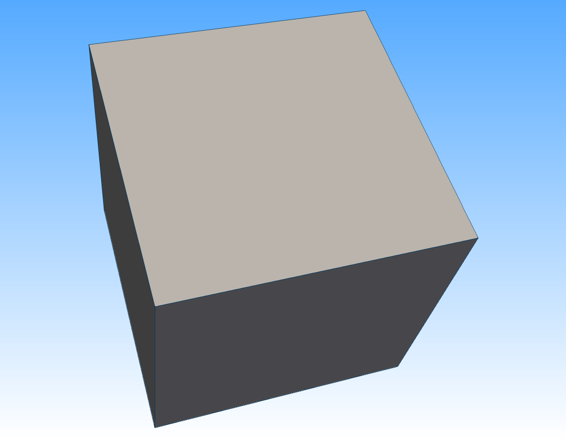
(a)

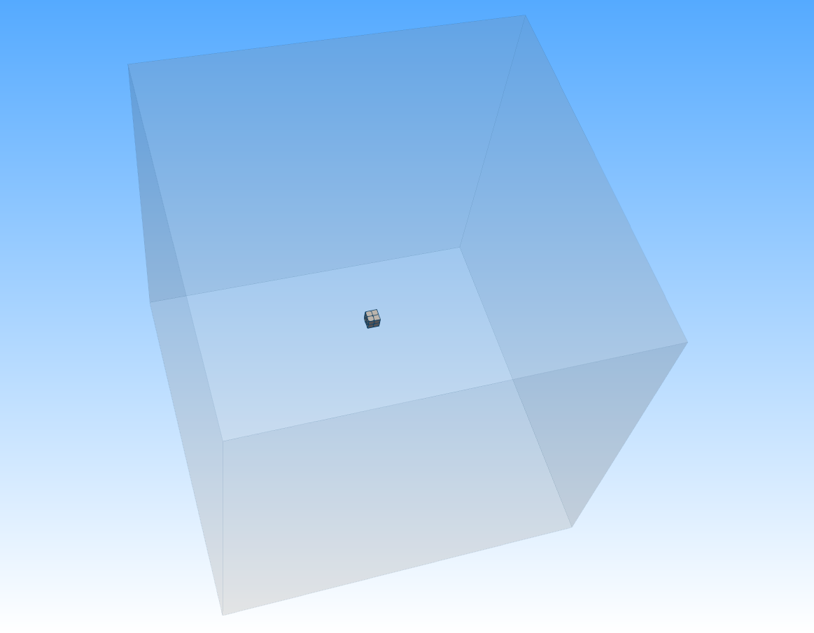
(b)

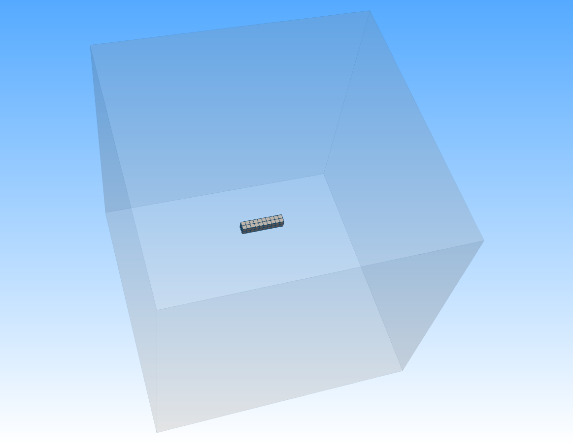
(c)

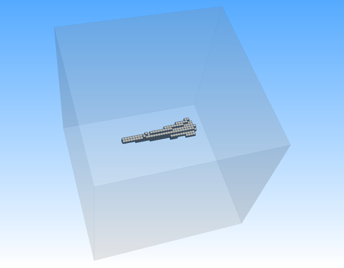
(d)

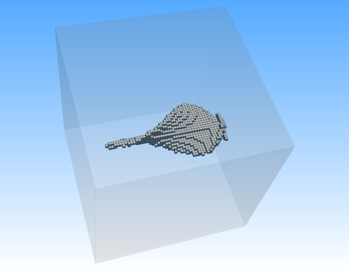
(e)

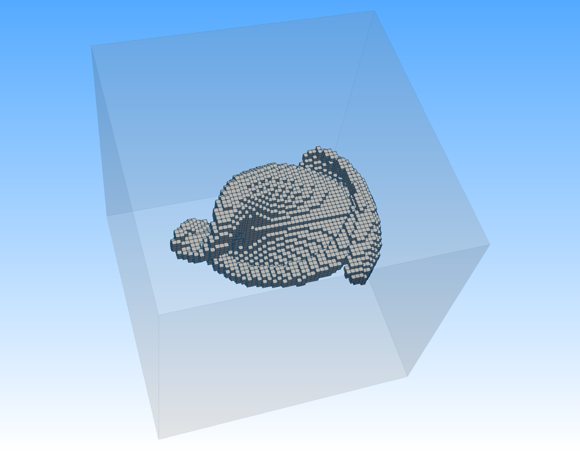
(f)

Figure 2. (a) Initial box $Q\supset A_{k}$. (b) Let $C\in{\mathcal{P}}_{s}$ be the box containing $p=R(u^{*})$ ($\ell=0$). (c) First continuation step. (d)-(f) Repeat step (c) with those boxes that are contained in the previous covering until no additional boxes were marked. A detailed discussion of the underlying dynamical system can be found in Section 5.1.3.

Intuitively it is clear that the algorithm, as constructed, generates an approximation of the embedded unstable manifold $W^{u}(p)$. In particular, we expect that the bigger $s$ and $\ell$ are the better the approximation will be.

Proposition 5.

1. The sets $C_{j}^{(\ell)}$ are coverings of $W_{j}$ for all $j,\ell=0,1,\ldots$. Moreover, for fixed $j$, we have

   $$\bigcap_{\ell=0}^{\infty}C_{j}^{(\ell)}=W_{j}.$$

2. Suppose that $\overline{W^{u}(p)}$ is linearly attractive, i.e., there is a $\lambda\in(0,1)$ and a neighborhood $U\supset Q\supset\overline{W^{u}(p)}$ such that

   $$\text{{dist}}\left(\varphi(y),\overline{W^{u}(p)}\right)\leq\lambda\leavevmode\nobreak\ \text{{dist}}\left(y,\overline{W^{u}(p)}\right)\quad\forall y\in U.$$ (19)

   Then the box coverings obtained by Algorithm 1 converge to the closure of the embedded unstable manifold $\overline{W^{u}(p)}$. That is,

   $$\bigcap_{\ell=0}^{\infty}G_{\ell}=\overline{W^{u}(p)}.$$

Proof.

1. Applying the subdivision algorithm with $\ell$ subdivision steps to the initial covering ${{\mathcal{B}}_{0}=\{C\}}$, we obtain ${\mathcal{B}}_{\ell}\subset{\mathcal{P}}_{s+\ell}$ of $A_{C}$, that is,

   $$A_{C}\subset\bigcup_{B\in{\mathcal{B}}_{\ell}}B.$$

   Here we assume that the subdivision scheme is creating coverings using elements from the partitions ${\mathcal{P}}_{n}$. By Proposition 4 (b) $A_{C}=W_{loc}^{u}(p)$ and by Proposition 2 the box coverings converge to $A_{C}$ for $\ell\rightarrow\infty$. Therefore, $A_{C}=W_{loc}^{u}(p)=W_{0}$ for $\ell\to\infty$. Since $j$ is fixed a continuity argument shows that the sets $C_{j}^{(\ell)}$ converge to $W_{j}$ for $\ell\rightarrow\infty$, i.e.,

   $$\bigcap_{\ell=0}^{\infty}C_{j}^{(\ell)}=W_{j}.$$

2. For each $\ell$ Algorithm 1 yields a covering of $\overline{W^{u}(p)}$, and therefore

   $$\bigcap_{\ell=0}^{\infty}G_{\ell}\supset\overline{W^{u}(p)}.$$

   Suppose there is $x\in\bigcap_{\ell=0}^{\infty}G_{\ell}\setminus\overline{W^{u}(p)}$. Since $\overline{W^{u}(p)}$ is compact, it follows that $\text{{dist}}\left(x,\overline{W^{u}(p)}\right)>0$. By definition of $x$, Algorithm 1 generates a $\mbox{diam}({\mathcal{B}}_{\ell})$-pseudo orbit $\{x_{0},\ldots,x_{j(\ell)}\}$ for each $\ell\geq 0$, where $x_{j(\ell)}=x$. That is

   $$x_{j}\in C_{j}^{(\ell)}\mbox{ and }\varphi(x_{j})\in{\mathcal{P}}_{s+\ell}(x_{j+1})\quad\forall j\in\{0,\ldots,j(\ell)-1\}.$$

   Here ${\mathcal{P}}_{s+\ell}(x_{j+1})\subset C_{j+1}^{(\ell)}$ denotes the element of ${\mathcal{P}}_{s+\ell}$ containing $x_{j+1}\in C_{j+1}^{(\ell)}$ and $j(\ell)=\min\{j\in\{0,\ldots,J_{\ell}\}:x\in C_{j}^{(\ell)}\}$, i.e., for each $j\geq j(\ell)$ continuation steps $x$ is covered. Observe that the sequence $j(\ell)$ is monotonically increasing in $\ell$ (cf. Step 3 of Algorithm 1 and Remark 4) and

   $$\|{x_{j}-\varphi(x_{j-1})}\|\leq\mathop{\rm diam}\nolimits(B_{\ell})\quad\forall j\in\{0,\ldots,j(\ell)-1\}.$$ (20)

   We first show by contradiction that $j(\ell)$ is unbounded. Suppose that $j(\ell)$ is bounded by some $J\in\mathbb{N}_{0}$, i.e., $\max{j(\ell)}=J$. Hence, by monotony of $j(\ell)$ there is $\ell_{0}\in\mathbb{N}_{0}$ such that $j(\ell)=J$ for all $\ell\geq\ell_{0}$. Using Remark 4 (a) we have

   $$x\in\left(\bigcap_{\ell=0}^{\ell_{0}-1}C_{j(\ell)}^{(\ell)}\right)\cap\left(\bigcap_{\ell=\ell_{0}}^{\infty}C_{J}^{(\ell)}\right)\subset\bigcap_{\ell=\ell_{0}}^{\infty}C_{J}^{(\ell)}=\bigcap_{\ell=0}^{\infty}C_{J}^{(\ell)}.$$

   However, by Proposition 5 (a) it follows that $x\in W_{J}\subset\overline{W^{u}(p)}$ which is a contradiction to $\text{{dist}}\left(x,\overline{W^{u}(p)}\right)>0$. Thus, $j(\ell)$ is unbounded.

   By assumption $\overline{W^{u}(p)}$ is linearly attractive in a neighborhood $U$. Hence, we can use (19) and (20) on the $\mbox{diam}({\mathcal{B}}_{\ell})$-pseudo orbit $\{x_{0},\ldots,x_{j(\ell)}\}$, where $x_{j(\ell)}=x$, in combination with the triangle inequality to obtain

   $$\text{{dist}}\left(x,\overline{W^{u}(p)}\right) \leq\text{{dist}}\left(\varphi(x_{j(\ell)-1}),\overline{W^{u}(p)}\right)+\mathop{\rm diam}\nolimits({\mathcal{B}}_{\ell})$$

   $$\leq\lambda\leavevmode\nobreak\ \text{{dist}}\left(x_{j(\ell)-1},\overline{W^{u}(p)}\right)+\mathop{\rm diam}\nolimits({\mathcal{B}}_{\ell})$$

   $$\ \vdots$$

   $$\leq\lambda^{j(\ell)}\leavevmode\nobreak\ \text{{dist}}\left(x_{0},\overline{W^{u}(p)}\right)+\mathop{\rm diam}\nolimits({\mathcal{B}}_{\ell})\sum_{i=0}^{j(\ell)-1}\lambda^{i}$$

   $$\leq\lambda^{j(\ell)}\leavevmode\nobreak\ \text{{dist}}\left(x_{0},\overline{W^{u}(p)}\right)+\frac{\mathop{\rm diam}\nolimits({\mathcal{B}}_{\ell})}{1-\lambda}\quad\longrightarrow 0\mbox{ for }\ell\rightarrow\infty.$$

   Here the last expression converges to zero because $\lambda\in(0,1)$ and $\mathop{\rm diam}\nolimits({\mathcal{B}}_{\ell})$ converges to zero for $\ell\rightarrow\infty$ (see (10)). Again we have an contradiction to $\text{{dist}}\left(x,\overline{W^{u}(p)}\right)>0$. It follows that

   $$\bigcap_{\ell=0}^{\infty}G_{\ell}\subset\overline{W^{u}(p)},$$

   which yields the desired statement.

∎

Remark 5.

1. If (16) would not be satisfied, then it can in general not be guaranteed that the continuation method leads to an approximation of the entire set $\overline{W^{u}(p)}$ or even ${\overline{W^{u}(p)}\cap Q}$. Rather it has to be expected that this is not the case. The reason is that the embedded unstable manifold $W^{u}(p)$ may ’leave’ $Q$ but may as well ’wind back’ into it. In this scenario the continuation method, as described above, will not cover all of $\overline{W^{u}(p)}\cap Q$. This situation is illustrated in Fig. 3 (a).

2. The assumption in Proposition 5 (b) is, for instance, not satisfied if $\overline{W^{u}(p)}$ forms a heteroclinic connection between the steady state solution $p$ and another unstable hyperbolic steady state $q$. In fact, in this case the algorithm would also generate a covering of the embedded unstable manifold of $q$. This situation is illustrated in Fig. 3 (b).

3. If (19) is not satisfied, but $\overline{{\mathcal{W}}_{\Phi}^{u}(u^{*})}$ is attractive, one can apply the subdivision scheme introduced in [9] to $G_{\ell}$ in order to approximate $\overline{W^{u}(p)}$ more accurately (cf. Proposition 3 (b)).

4. Note that (19) is satisfied if the observation map $R$ is bi-Lipschitz with Lipschitz constant $L\geq 1$ and $\overline{{\mathcal{W}}_{\Phi}^{u}(u^{*})}$ is linearly attractive with $\lambda\in(0,L^{-2})$.

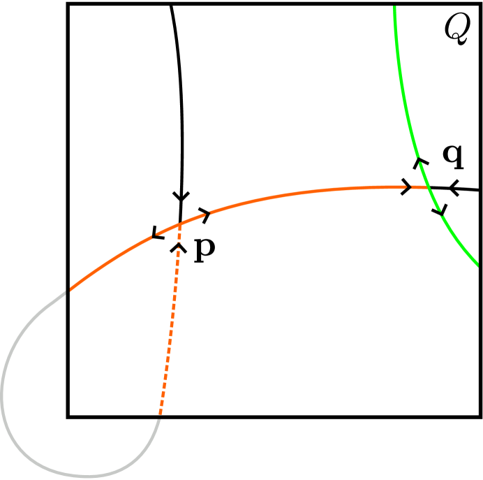
(a)

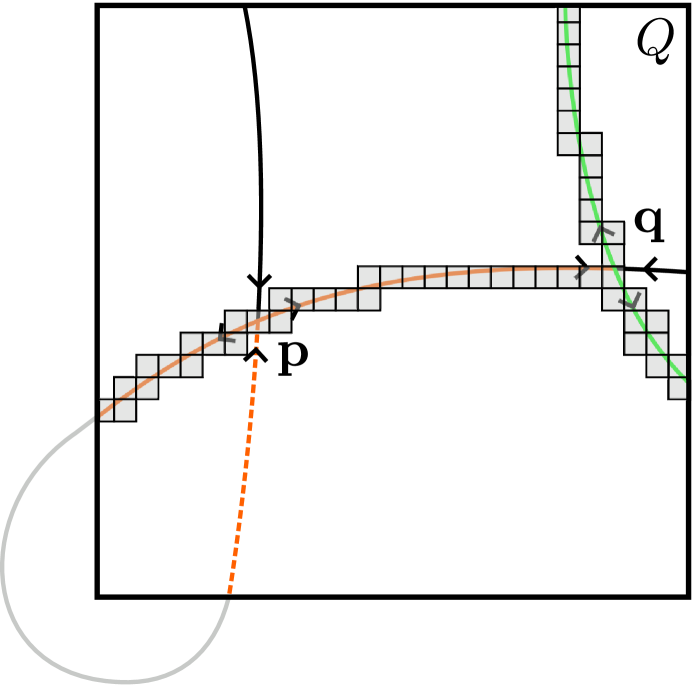
(b)

Figure 3. Illustration of the possible situations discussed in Remark 5 (a) and (b).
(a) The dashed line will not be covered by the continuation method and thus, we will not approximate the entire set $W^{u}(p)\cap Q$. (b) Schematic box covering obtained by the continuation method, where in this particular case we also obtain a covering of $W^{u}(q)\cap Q$.

4. Numerical realization of the CDS $\varphi$ for partial differential equations

As discussed in the introduction, dynamical systems with infinite dimensional state space, but finite dimensional attractors arise in particular in two areas of applied mathematics, namely dissipative partial differential equations and delay differential equations with small constant time delay. In this article we will focus on the PDE case, and we will present one specific realization of the maps $R$ and $E$ for this situation.

More precisely, we will consider explicit differential equations of the form

$$\frac{\partial}{\partial t}u(y,t)=F(y,u),\leavevmode\nobreak\ u(y,0)=u_{0}(y),$$ (21)

where $u:\mathbb{R}^{n}\times\mathbb{R}\rightarrow\mathbb{R}^{n}$ is in some Banach space $Y$ and $F$ is a (nonlinear) differential operator. We assume that the dynamical system $\eqref{eq:PDE}$ has a well-defined semiflow on $Y$.

In order to numerically realize the construction of the map $\varphi=R\circ\Phi\circ E$ described in Section 2.2, we have to work on three tasks: the implementation of $E$, the implementation of $R$, and the realization of the time-$T$-map of (21), denoted by $\Phi$, respectively. For the latter we will rely on standard methods for forward time integration of PDEs, e.g., a fourth-order time stepping method for the one-dimensional Kuramoto-Sivashinsky equation [29]. Observe that the numerical realization of $\Phi$ strongly depends on the underlying PDE. The map $R$ will be realized on the basis of Theorem 2.2 or Remark 1, respectively. For the numerical construction of the continuous map $E$ we will present a new method that uses statistical information from previous computations. This step is in particular crucial for the continuation step, since we want to restart the algorithm with initial conditions that satisfy the identities

$$(E\circ R)(u)=u\quad\forall u\in\mathcal{W}_{\Phi}^{u}(u^{*})\quad\text{ and }\quad(R\circ E)(x)=x\quad\forall x\in W^{u}(p).$$

(cf. (5)) at least approximately.

From now on we assume that upper bounds for both the box counting dimension $d$ and the thickness exponent $\sigma$ are available. This allows us to fix $k>2(1+\sigma)d$ according to Remark 1.

4.1. Numerical realization of $R$

In [9] $R$ has been defined on the basis of Theorem 2.3, where function evaluations at a fixed time have been used. Thus, in the case of scalar delay differential equations $R$ has been defined as the delay coordinate map

$$R=D_{k}[f,\Phi](u)=(u(-\tau),\Phi(u)(-\tau),\ldots,\Phi^{k-1}(u)(-\tau))^{T},$$ (22)

where $\tau>0$ is the constant time-delay of the underlying DDE. In principle it would also be possible to observe the evolution of a partial differential equation by a delay coordinate map. However, from a computational point of view this would be very inefficient. The reason is that for the realization of the map ${E:\mathbb{R}^{k}\to Y}$ one would have to reconstruct functions from time delay coordinates. Thus, for each point in observation space one would essentially have to store the entire corresponding function. To overcome this problem, in this work we will present a different approach. In what follows, we will assume that the function $u\in Y$ can be represented in terms of an orthonormal basis $\{\Psi_{i}\}_{i=1}^{\infty}$, i.e.,

$$u(y,t)=\sum_{i=1}^{\infty}x_{i}(t)\Psi_{i}(y),$$ (23)

where the $\Psi_{i}$ are elements from a Hilbert space (e.g., $L^{2}$). Then our observation map $R$ will be defined by projecting a function onto $k$ coefficients $x_{i}$ of its Galerkin expanion. For the approximation of $u$, i.e.,

$$u(y,t)\approx\sum_{i=1}^{S}x_{i}(t)\Psi_{i}(y)$$ (24)

we want to use an optimal basis $\{\Psi_{i}\}_{i=1}^{S}$ (i.e., as small as possible) in the sense that it contains the ’most characteristic’ data from an ensemble of functions. The notion ’most characteristic’ implies the use of an averaging operation. Furthermore, this basis has to be capable of representing the solution $u\in Y$ of the underlying PDE (21) with a small error. Both requirements can be addressed by the proper orthogonal decomposition (POD) (c.f. [43, 1, 23]), also known as the principal component analysis or the Karhunen-Loève transformation. In order to compute a basis $\{\Psi_{i}\}$ for $i=1,\ldots,S$ and $S>k$, we first generate time-snapshots of a long-time simulation for some set of initial conditions of the underlying PDE. Then we approximate the POD-basis via the singular value decomposition (e.g., [4, 35, 46]). Using this basis we then approximate $u\in Y$ by (24) where $x_{i}(t)$ denotes the $i$-th POD-coefficient at time $t$.

Given the basis $\{\Psi_{i}\}_{i=1}^{S}$ and using the fact that this basis is orthogonal, we then define the observation map by choosing $k$ different observables

$$f_{i}(u)=\langle u,\Psi_{i}\rangle=x_{i}\quad\mbox{for }i=1,\ldots,k.$$ (25)

This yields

$$R(u)=(f_{1}(u),\ldots,f_{k}(u))^{\top}=(x_{1},\ldots,x_{k})^{\top}.$$ (26)

Observe that $R$ is linear and bounded and hence, for $k$ sufficiently large, Theorem 2.2 and Remark 1, respectively, guarantee that generically (in the sense of prevalence) $R$ will be a one-to-one map on $\mathcal{A}$.

4.2. Numerical realization of $E$

In the application of the continuation scheme for the computation of embedded unstable manifolds $W^{u}(p)$ described in Section 3 one has to perform the continuation step

$${\mathcal{C}}_{j+1}^{(\ell)}=\left\{B\in{\mathcal{P}}_{s+\ell}:\exists B^{\prime}\in{\mathcal{C}}_{j}^{(\ell)}\mbox{ such that }B\cap\varphi(B^{\prime})\neq\emptyset\right\}$$

(see (17)). Numerically this is realized as follows: At first $\varphi$ is evaluated for a large number of test points $x\in B^{\prime}$ for each box $B^{\prime}\in{\mathcal{C}}_{j}^{(\ell)}$. Then a box $B\in{\mathcal{P}}_{s+\ell}$ is added to the collection ${\mathcal{C}}_{j+1}^{(\ell)}$ if there is a least one $x\in B^{\prime}$ such that $\varphi(x)\in B$.

Remark 6.

In practice the test points $x\in B^{\prime}$ can be chosen according to several different strategies: In low dimensional problems one can choose them from a regular grid within each box $B$. Alternatively one can select the test points from the boundaries of the boxes. In our computations we use a Monte Carlo sampling.

By Section 4.1 the state space for the CDS $\varphi$ is given by points $x\in\mathbb{R}^{k}$ where $x_{1},\ldots,x_{k}$ are the POD-coefficients. For the evaluation of $\varphi=R\circ\Phi\circ E$ at a test point $x$ we need to define the image $E(x)$, that is, we need to generate adequate initial conditions for the forward integration of the PDE (21). In the first step of the continuation method we proceed as follows. Given the POD-basis $\{\Psi_{i}\}$ for $i=1,\ldots,S$ and $S>k$, we simply construct initial conditions $u=E(x)$ near the unstable (hyperbolic) steady state by defining the map $E$ as

$$E(x)=\sum_{i=1}^{k}x_{i}\Psi_{i}.$$ (27)

Observe that by this choice of $E$ and $R$ both conditions $(R\circ E)(x)=x$ and ${(E\circ R)(u)=u}$ are satisfied for each test point $x\in{\mathcal{C}}_{0}^{(\ell)}$ (see (5) and (26)). Then we use the time-$T$-map $\Phi$ of the underlying PDE to obtain a function $\bar{u}=\Phi(E(x))$. If $k$ is not sufficiently large, then $(E\circ R)(\bar{u})=\bar{u}$ will in general not be satisfied anymore. Therefore, it is possible that initial conditions $u=E(x)$ for $x\in{\mathcal{C}}_{j+1}^{(\ell)}$, $j=0,1,\ldots$, generated by (27) are not even close to the unstable manifold. This is not acceptable since the requirement $(E\circ R)(u)=u$ for all $u\in{\mathcal{W}}_{\Phi}^{u}(u^{*})$ (see (5)) is crucial in order to compute a reliable covering of the embedded unstable manifold.

To enforce this equality at least approximately we extend the expansion and construct initial functions by

$$E(x)=\sum_{i=1}^{k}x_{i}\Psi_{i}+\sum_{l=k+1}^{S}x_{l}\Psi_{l}.$$ (28)

Here only the first $k$ POD-coefficients are given by the coordinates of points inside $B\subset\mathbb{R}^{k}$. Thus, it remains to discuss how to choose the POD-coefficients $x_{k+1},\ldots,x_{S}$. The idea is to use a new heuristic strategy that utilizes statistical information obtained in the previous continuation step: Suppose we want to evaluate $\varphi$ for a large number of test points $x$ in a box $B\in{\mathcal{C}}_{j+1}^{(\ell)}$. By the continuation step (cf. Algorithm 1), there must have been at least one ${\hat{B}\in{\mathcal{C}}_{j}^{(\ell)}}$ such that $\bar{x}=R(\Phi(E(\hat{x})))\in B$ for at least one test point $\hat{x}\in\hat{B}$. For all these points $\bar{x}$ we can compute the POD-coefficients $\bar{x}_{k+1},\ldots,\bar{x}_{S}$ by

$$\bar{x}_{i}=\langle\Phi(E(\hat{x})),\Psi_{i}\rangle,\quad i=k+1,\ldots,S.$$

Then we sample the box $B$ with all points $\bar{x}$ for which additional information is available. However, the number of these points $\bar{x}$ might be too small, such that $B$ is not discretized sufficiently well and we have to generate additional test points. For this, we first choose a certain number of points $\widetilde{x}\in B$ at random. Then we extend these points to elements in $\mathbb{R}^{S}$ as follows: We first compute componentwise the mean value $\mu_{i}$ and the variance $\sigma_{i}^{2}$ of all POD-coefficients $\bar{x}_{i}$, for $i=k+1,\ldots,S$. This allows us to make a Monte Carlo sampling for the additional coefficients of $\widetilde{x}_{i}$ for $i=k+1,\ldots,S$, i.e.,

$$\widetilde{x}_{i}\sim\mathcal{N}(\mu_{i},\sigma_{i}^{2})\quad\mbox{ for }i=k+1,\ldots,S.$$

Finally, we compute initial functions of the form

$$E(\widetilde{x})=\sum_{i=1}^{S}\widetilde{x}_{i}\Psi_{i}.$$

By this construction we expect in each continuation step to generate initial functions that satisfy an approximation of the identity $(E\circ R)(u)=u$ for all $u\in{\mathcal{W}}_{\Phi}^{u}(u^{*})$. We will illustrate our statistical approach in the next section for the one-dimensional Kuramoto-Sivashinsky equation.

5. Numerical results

In this section we present results of computations carried out for the Mackey-Glass delay differential equation and the Kuramoto-Sivashinsky equation, respectively. For the numerical realization of the CDS $\varphi$ for delay differential equations the reader is referred to [9].

5.1. The Kuramoto-Sivashinsky equation

We start with the well-known
Kuramoto-Sivashinsky equation in one spatial dimension which is given by

$$u_{t}+\nu u_{yyyy}+u_{yy}+\frac{1}{2}(u_{y})^{2}=0,\quad 0\leq y\leq L,$$ (29)

$$u(y,0)=u_{0}(y),\quad u(y+L,t)=u(y,t).$$

This equation has been studied extensively over the past $40$ years. It has, for instance, been used to model phase dynamics in reaction-diffusion systems [34] or small thermal diffusive instabilities in laminar flame fronts [44]. Following [25, 30], we normalize the K-S equation to an interval length of $2\pi$ and set the damping parameter to the original value derived by Sivashinsky, i.e., $\nu=4$. Then equation (LABEL:eq:KS) can be written as

$$u_{t}+4u_{yyyy}+\mu\left[u_{yy}+\cfrac{1}{2}(u_{y})^{2}\right]=0,\quad 0\leq y\leq 2\pi,$$ (30)

$$u(y,0)=u_{0}(y),\quad u(y+2\pi,t)=u(y,t).$$

In equation (LABEL:eq:KS_normalized) we introduce a new parameter $\mu=L^{2}/4\pi^{2}$, where $L$ denotes the size of a typical pattern scale (cf. (LABEL:eq:KS)). In [25, 30] numerical and analytical studies were made by varying $\mu$ over a finite interval, showing the complex hierarchy of bifurcations. We are in particular interested in computing the unstable manifold of the trivial unstable steady state for different parameter values $\mu$. In order to use our algorithm developed in Section 3 it is crucial to have a good estimate of the dimension of the invariant set $\mathcal{A}$ and ${\mathcal{W}}_{\Phi}^{u}(y)$, respectively (cf. Section 2). In [39] it has been shown that the dimension of the inertial manifold of (LABEL:eq:KS) for $\nu=1$ is $d\leq L^{2.46}$, i.e., each invariant set has finite dimension. However, these estimates are very pessimistic and we expect that we will obtain one-to-one images of the unstable manifold for smaller related embedding dimensions $k$.

In what follows, the observation space is defined through projections onto the first $k$ POD-coefficients. For each parameter value $\mu$ we compute the POD-basis by using the snapshot-matrix obtained through a long-time integration with the initial condition

$$u_{0}(y)=10^{-4}\cdot\cos\left(y\right)\cdot\left(1+\sin\left(y\right)\right)$$

(cf. Section 4.1).

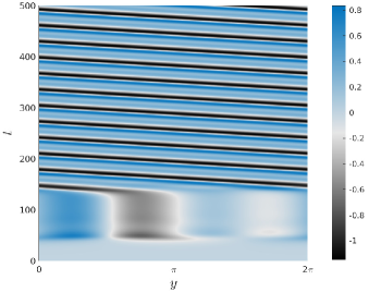
(a) Direct simulation

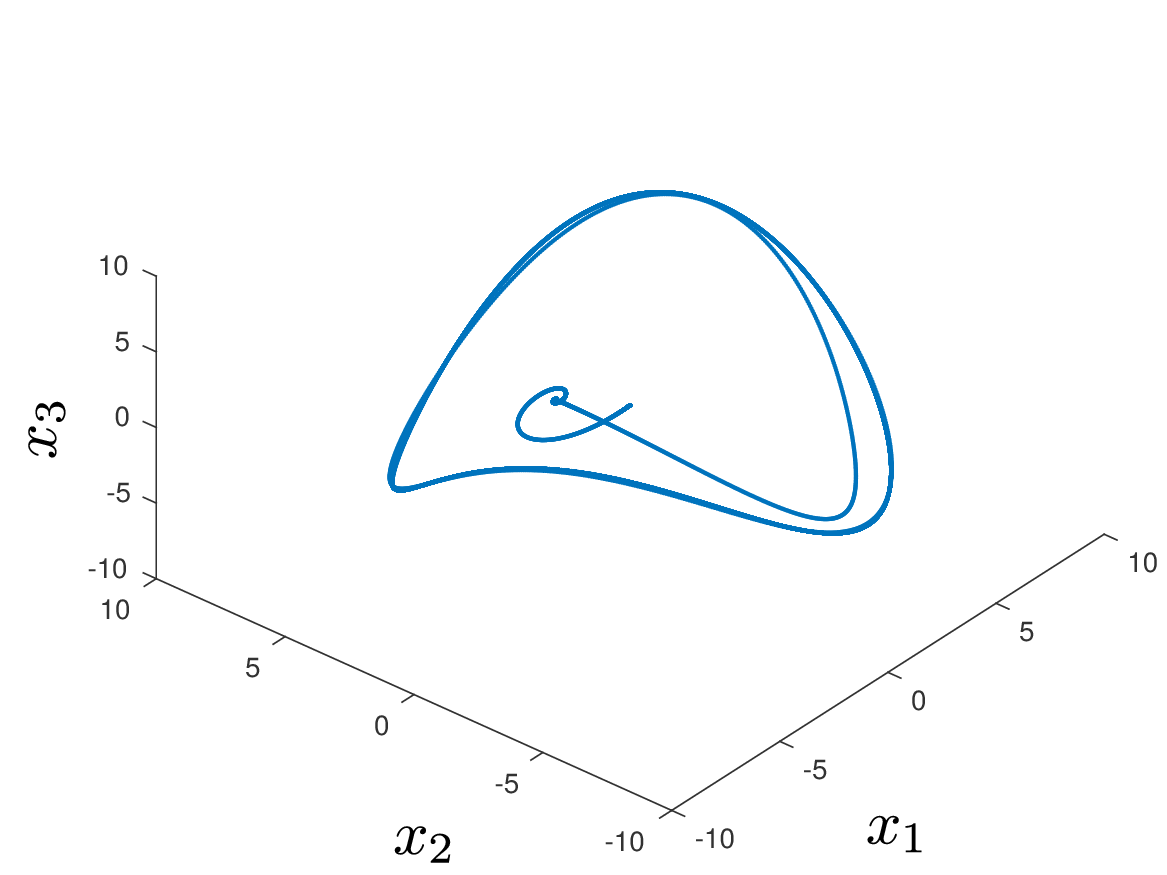
(b) Observation space

Figure 4. (a) Direct simulation of the Kuramoto-Sivashinsky equation for $\mu=15$. The initial value is attracted to a traveling wave solution; (b) Corresponding embedding in observation space. As expected the CDS possesses a related limit cycle.

5.1.1. The traveling wave

For the parameter value $\mu=15$ the Kuramoto-Sivashinsky equation possesses a stable traveling wave solution (cf. Fig. 4 (a)). Due to the symmetry imposed by the periodic boundary conditions there are two waves traveling in opposite directions [30]. Correspondingly the CDS possesses for each traveling wave a limit cycle in observation space (cf. Fig. 4 (b)). We expect that the dimension of the embedded unstable manifold is approximately two since different initial conditions result in trajectories in observation space that are rotations of each other about the origin.

By choosing the embedding dimension $k=7$ we restrict the initial functions in the first continuation step to the subspace that is spanned by the first seven POD-modes and since $d(\overline{W^{u}(p)};\mathbb{R}^{k})\approx 2$, we expect to obtain a one-to-one image of ${\mathcal{W}}_{\Phi}^{u}(u^{*})$. In Fig. 5 we show a comparison of the numerical realization of the continuous map $E$ with initial functions generated by (27), i.e., where $x_{k+1}=\ldots=x_{S}=0$ for all test points $x$ (red) and the statistical approach discussed in Section 4.2 (blue). By using only $k=3$ POD-coefficients, we construct initial functions that by far do not satisfy $(E\circ R)(u)=u$.

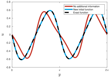
Figure 5. Illustration of the numerical realization of $E$ for the Kuramoto-Sivashinsky equation for $\mu=15,\ k=3$ and $S=13$ in one specific box $B$ after at least one continuation step: The black function represents $\Phi(E(\hat{x}))$ from the previous continuation step; the red function is generated by (27); the blue function is generated by (28), where we use additional statistical information for the POD-coefficients $x_{k+1},\ldots,x_{S}$.

We choose $Q=[-8,8]^{7}$ and initialize a fine partition ${\mathcal{P}}_{s}$ of $Q$ for $s=21,35,49,63$. Next we set $T=200$. In addition, we define a finite time grid $\{t_{0},\ldots,t_{N}\}$, where $t_{N}=T$, and mark all boxes that are hit in each time step (a similar approach has been used in [28]). This strategy will be used for each example in this section.

In Fig. 6 (a)-(d) we illustrate successively finer box coverings of the unstable manifold as well as a transparent box covering depicting the complex internal structure of the unstable manifold. Observe that the boundary of the unstable manifold consists of two limit cycles which are symmetric in the first POD-coefficient $x_{1}$. This is due to the fact that the Kuramoto-Sivashinsky equation with periodic boundary conditions (LABEL:eq:KS_normalized) possesses $O(2)$-symmetry.

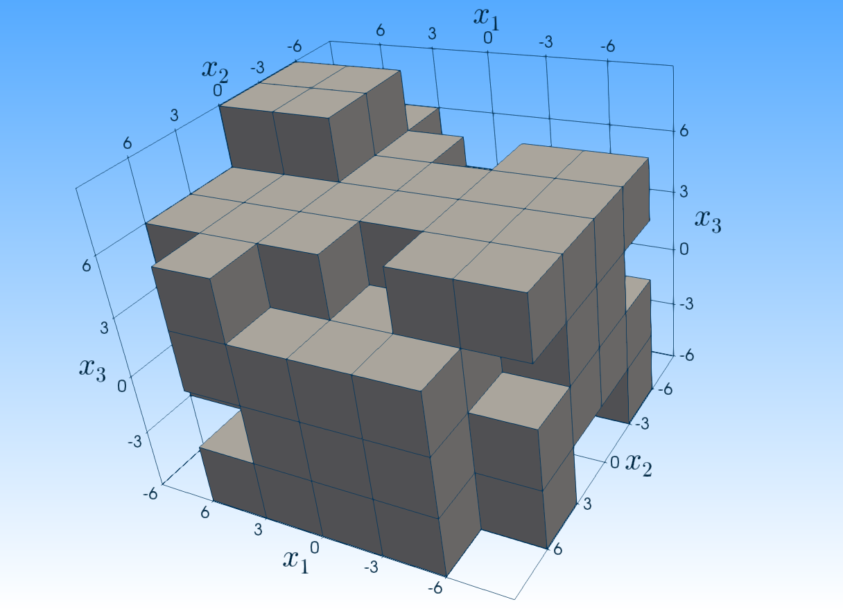
(a) $s=21$ and $\ell=0$

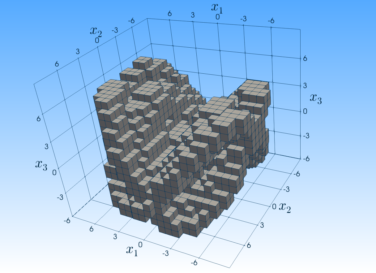
(b) $s=35$ and $\ell=0$

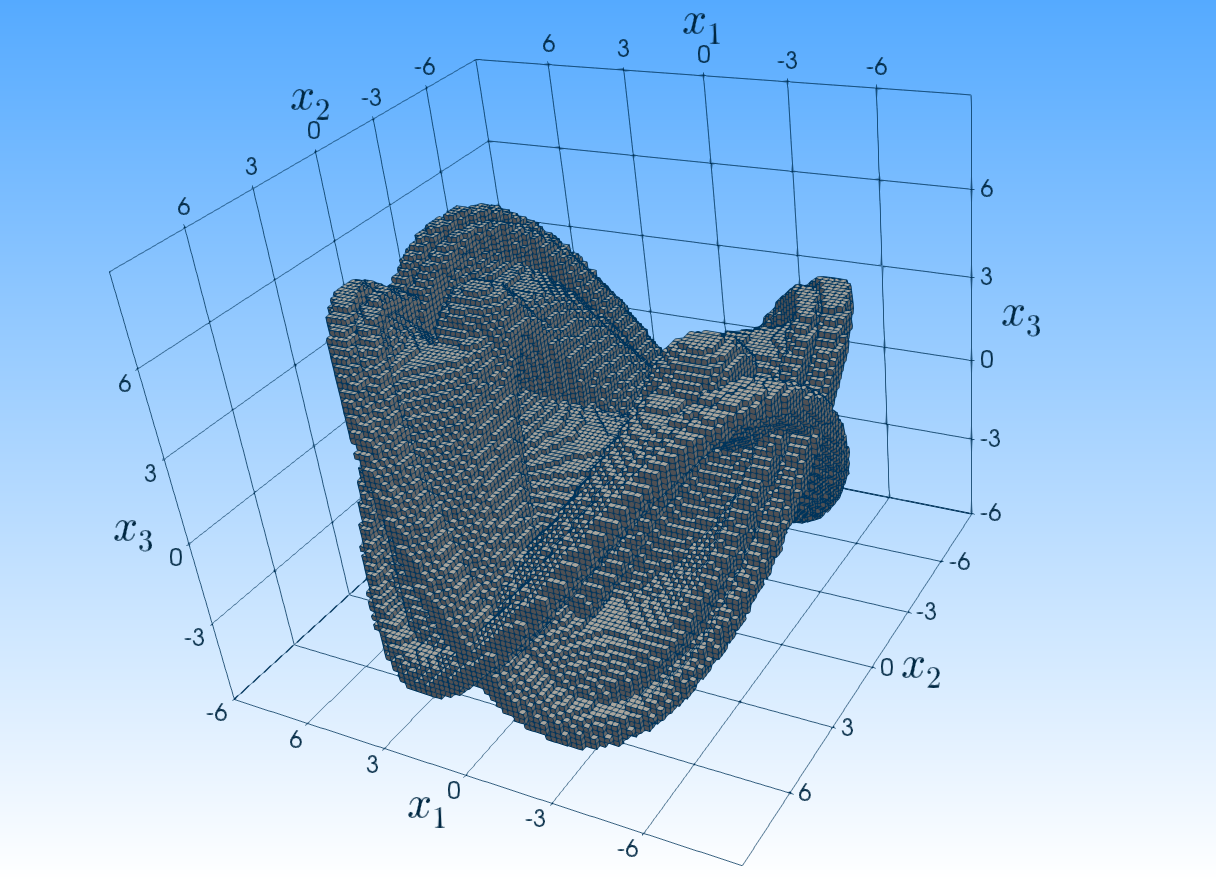
(c) $s=49$ and $\ell=0$

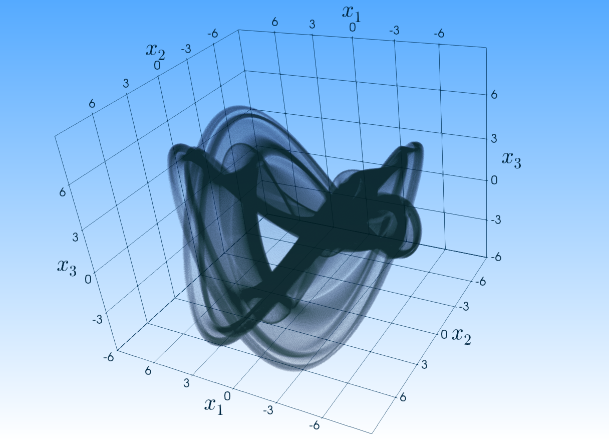
(d) $s=63$ and $\ell=0$

Figure 6. (a)-(d) Successively finer box-coverings of the unstable manifold for $\mu=15$. (d) Transparent box covering for $s=63$ and $\ell=0$ depicting the internal structure of the unstable manifold.

5.1.2. The stable heteroclinic cycle

For $\mu=18$, the observed long-term behavior consists of a pulsation between two states, which appear to be $\pi/2$-translations of each other. The transients linger close to one of these states for a comparatively long time before they pulse back to the other (cf. Fig. 7 (a)).

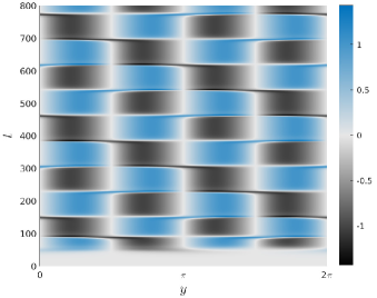
(a) Direct simulation

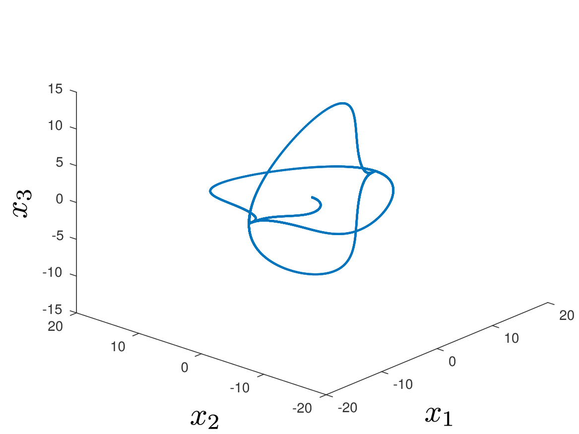
(b) Observation space

Figure 7. (a) Direct simulation of the Kuramoto-Sivashinsky equation for $\mu=18$; (b) Corresponding embedding in observation space depicting the stable heteroclinic loop.

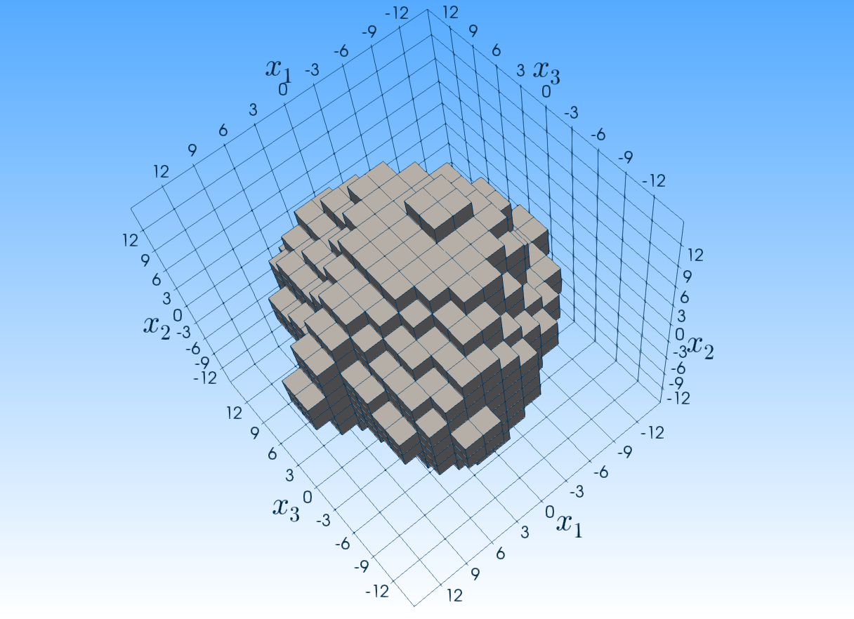
$s=12$ and $\ell=0$

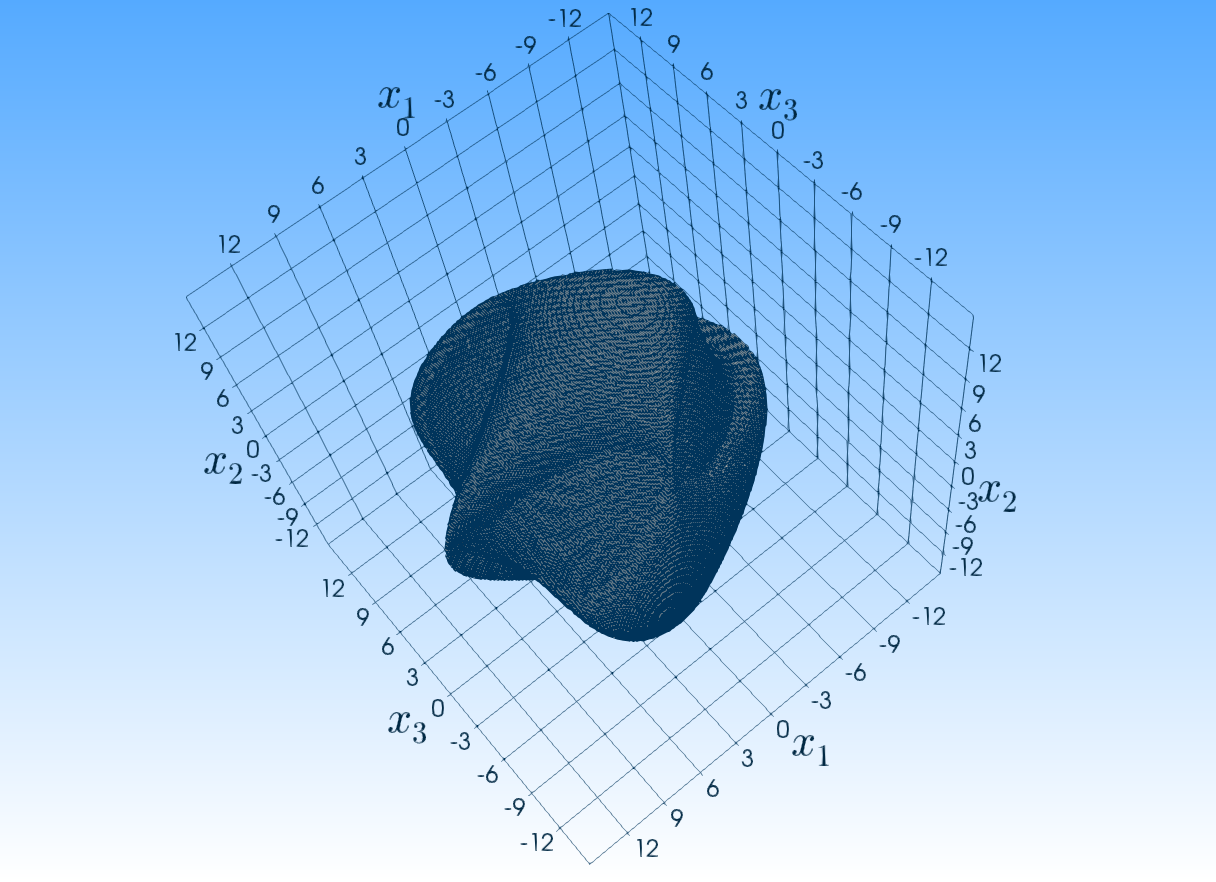
$s=24$ and $\ell=0$

Figure 8. (a)-(b) Successively finer box-coverings of the unstable manifold for $\mu=18$.

It was observed in [30] that the pulsation projected onto the $\cos(2x)$ and $\sin(2x)$ coefficient plane, respectively, appears as a straight line passing through the origin. In addition, different pulsations, resulting from different initial conditions, give straight lines that are rotations of each other about the origin. By projecting the pulsation onto the first three POD-coefficients, we observe a similar behavior in observation space. Thus, we expect that the unstable manifold will be of dimension at least three. The projection of the long time simulation (cf. Fig. 8 (a)) onto the first three POD-coefficients is shown in Fig. 7 (b).

For the initialization of Algorithm 1, we choose the embedding dimension $k=3$ and, therefore, restrict our initial functions to the function space generated by the first three POD-modes. Since the embedding dimension is too small, we expect to approximate just a projection of the unstable manifold. For a related discussion in the finite dimensional context we refer the interested reader to [41]. Moreover, we choose $Q=[-20,20]^{3}$ and set $T=200$. In Fig. 8 (a) and (b) we show two box coverings obtained by our continuation method for different values $s\in\mathbb{N}$ of the partition ${\mathcal{P}}_{s}$ of $Q$. As expected, we observe that the embedded unstable manifold appears to be a solid three-dimensional object. This corresponds to the observation mentioned above.

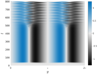
(a) Direct simulation

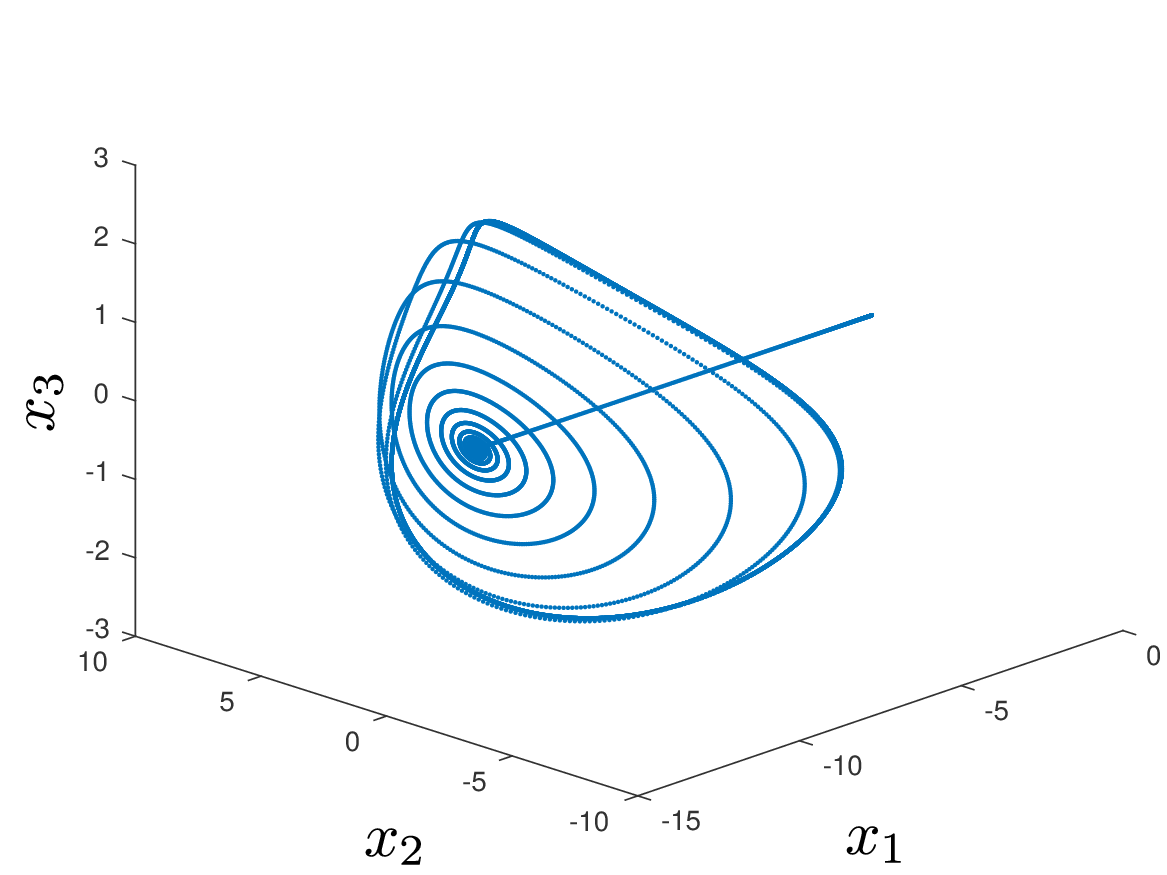
(b) Observation space

Figure 9. (a) Direct simulation of the Kuramoto-Sivashinsky equation for $\mu=32$; (b) Corresponding embedding in observation space.

5.1.3. The Oseberg transition

In the last example we have chosen $\mu=32$. In Fig. 9 (a) and (b) we show a direct simulation as well as the corresponding embedding in the observation space. The initial condition $u_{0}$ is first attracted to an unstable so-called bimodal steady state, and eventually accumulates on a limit cycle as $t\rightarrow\infty$.

In Fig. 10 (a) and (b) we show successively finer box coverings of the unstable manifold obtained by our continuation method. We remark that already previously a similar result has been obtained by [26] which the authors called the Oseberg transition. In this work, the authors restricted the phase space to the invariant subspace of odd functions, in which the solutions can be represented by the Fourier series

$$u(y,t)=\sum_{j=1}^{\infty}b_{j}(t)\sin(jy),$$

where an eight-mode Galerkin truncation of the PDE was used. The restricted global attractor, illustrated through the first, second and third Fourier coefficients as observables, look qualitatively very similar to our unstable manifold illustrated in Fig. 10.

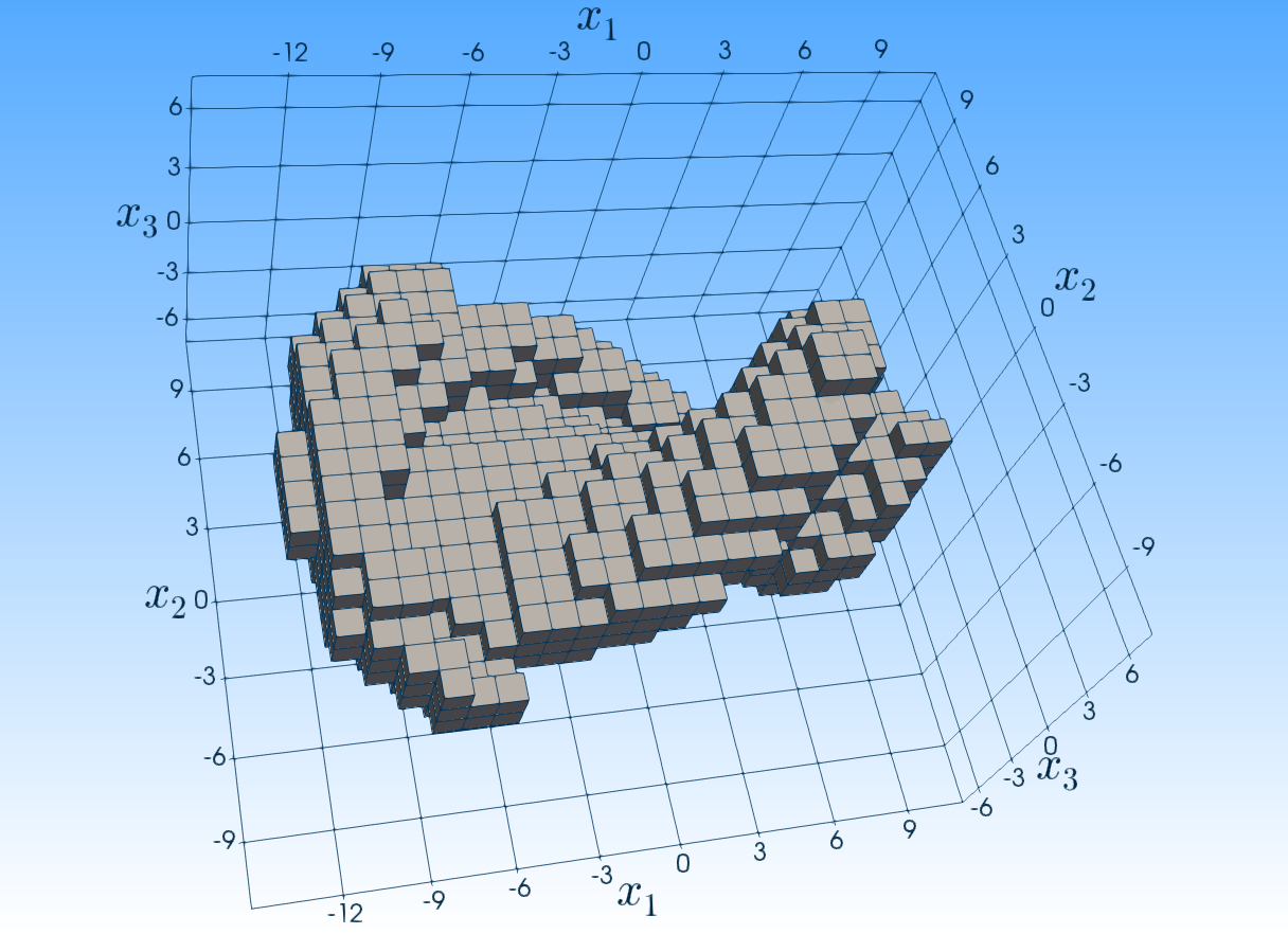
(a) $s=15$ and $\ell=0$

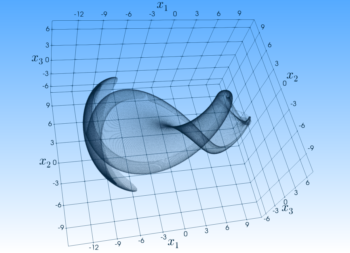
(b) $s=27$ and $\ell=0$

Figure 10. Successively finer box-coverings of the unstable manifold for $\mu=32$. Furthermore, in (b) we show a transparent box covering for $s=27$ and $\ell=0$ depicting the internal structure of the unstable manifold.

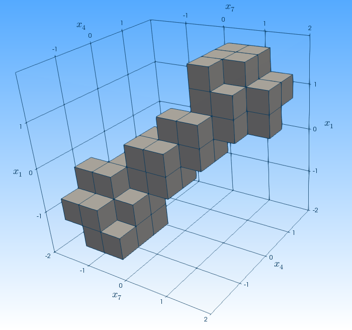
(a) $s=21$ and $\ell=0$

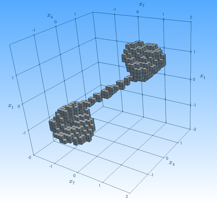
(b) $s=35$ and $\ell=0$

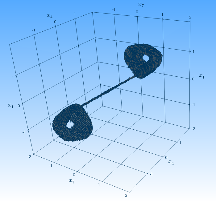
(c) $s=49$ and $\ell=0$

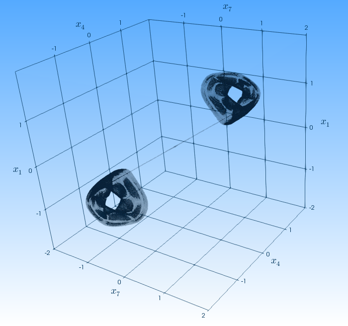
(d) $s=49$ and $\ell=14$

Figure 11. (a)-(c) Successively finer box-coverings of the unstable manifold of the Mackey-Glass equation (31). (d) Transparent box covering for $s=49$ and $\ell=14$.

5.2. The Mackey-Glass equation

Finally, we show the feasibility of our method by computing an unstable manifold for one delay differential equation with constant delay. Here, we consider the delay differential equation introduced by Mackey and Glass in 1977 [37] defined by

$$\dot{u}(t)=\beta\frac{u(t-\tau)}{1+u(t-\tau)^{\eta}}-\gamma u(t),$$ (31)

where we choose $\beta=2,\gamma=1$, $\eta=9.65$, and $\tau=2$. This equation is a model of blood production, where $u(t)$ represents the concentration of blood at time $t$, $\dot{u}(t)$ represents production at time $t$ and $u(t-\tau)$ is the concentration at an earlier time, when the request for more blood is made. This equation possesses an unstable steady state $u_{0}(t)=0$. To this end, we start the continuation method in ${p=R(u_{0})\in\mathbb{R}^{k}}$, where $R$ is defined by (22). Furthermore, we choose $k=7$ and $Q=[-1.5,1.5]^{7}\subset\mathbb{R}^{7}$.

In Fig. 11 (a) – (c), we show projections of the coverings obtained via the continuation method for $s=21,35,49$ ($\ell=0$ in all three cases). In addition, in Fig. 11 (d) we also show a transparent box covering for $s=49$ and $\ell=14$.

References

- [1] G. Berkooz, P. Holmes, and J. L. Lumley. The proper orthogonal decomposition in the analysis of turbulent flows. Annual Review of Fluid Mechanics, 25(1):539–575, 1993.
- [2] Andreas Bittracher, Péter Koltai, Stefan Klus, Ralf Banisch, Michael Dellnitz, and Christof Schütte. Transition manifolds of complex metastable systems. Journal of Nonlinear Science, 28(2):471–512, 2018.
- [3] J. Carr. Applications of centre manifold theory, volume 35. Springer Science & Business Media, 2012.
- [4] A. Chatterjee. An introduction to the proper orthogonal decomposition. Current Science, 78(7):808–817, 2000.
- [5] S. N. Chow and J. K. Hale. Methods of bifurcation theory, volume 251. Springer Science & Business Media, 2012.
- [6] S. N. Chow and K. Lu. Invariant manifolds for flows in Banach spaces. Journal of Differential Equations, 74(2):285–317, 1988.
- [7] P. Constantin, C. Foias, B. Nicolaenko, and R. Temam. Integral manifolds and inertial manifolds for dissipative partial differential equations. Springer-Verlag, 1988.
- [8] P. Constantin, C. Foias, and R. Temam. Attractors representing turbulent flows. Memoirs of the American Mathematical Society, 1985.
- [9] M. Dellnitz, M. Hessel-von Molo, and A. Ziessler. On the computation of attractors for delay differential equations. Journal of Computational Dynamics, 3(1):93–112, 2016.
- [10] M. Dellnitz and A. Hohmann. The Computation of Unstable Manifolds using Subdivision and Continuation. In Nonlinear Dynamical Systems and Chaos, pages 449–459. Springer, 1996.
- [11] M. Dellnitz and A. Hohmann. A subdivision algorithm for the computation of unstable manifolds and global attractors. Numerische Mathematik, 75:293–317, 1997.
- [12] M. Dellnitz and O. Junge. On the approximation of complicated dynamical behavior. SIAM Journal on Numerical Analysis, 36(2):491–515, 1999.
- [13] M. Dellnitz, O. Junge, M. Lo, J. E. Marsden, K. Padberg, R. Preis, S. Ross, and B. Thiere. Transport of Mars-crossing asteroids from the quasi-Hilda region. Physical Review Letters, 94(23):231102, 2005.
- [14] J. Dugundji. An extension of Tietze’s theorem. Pacific Journal of Mathematics, 1(3):353–367, 1951.
- [15] C. Foias, M. S. Jolly, I. G. Kevrekidis, G. R. Sell, and E. S. Titi. On the computation of inertial manifolds. Physics Letters A, 131(7):433–436, 1988.
- [16] G. Froyland and M. Dellnitz. Detecting and locating near-optimal almost invariant sets and cycles. SIAM Journal on Scientific Computing, 24(6):1839–1863, 2003.
- [17] G. Froyland, C. Horenkamp, V. Rossi, N. Santitissadeekorn, and A. Sen Gupta. Three-dimensional characterization and tracking of an Agulhas ring. Ocean Modelling, 52-53:69–75, 2012.
- [18] G. Froyland, S. Lloyd, and N. Santitissadeekorn. Coherent sets for nonautonomous dynamical systems. Physica D: Nonlinear Phenomena, 239:1527–1541, 2010.
- [19] C.M. Groothedde and J.D.M. James. Parameterization method for unstable manifolds of delay differential equations. Journal of Computational Dynamics, pages 340–367, 2017.
- [20] J. Hale. Functional Differential Equations, volume 3. Springer-Verlag, 1971.
- [21] J. K. Hale. Asymptotic Behavior of Dissipative Systems, volume 25. American Mathematical Society, 2010.
- [22] D. Henry. Geometric Theory of Semilinear Parabolic Equations, volume 840 of Lecture Notes in Mathematics. Springer-Verlag, 2006.
- [23] P. Holmes, J. L. Lumley, G. Berkooz, and C. W. Rowley. Turbulence, Coherent Structures, Dynamical Systems and Symmetry. Cambridge University Press, 2012.
- [24] B. R. Hunt and V. Y. Kaloshin. Regularity of embeddings of infinite-dimensional fractal sets into finite-dimensional spaces. Nonlinearity, 12(5):1263–1275, 1999.
- [25] J. M. Hyman, B. Nicolaenko, and S. Zaleski. Order and complexity in the Kuramoto-Sivashinsky model of weakly turbulent interfaces. Physica D: Nonlinear Phenomena, 23(1-3):265–292, 1986.
- [26] M. E. Johnson, M. S. Jolly, and I. G. Kevrekidis. The Oseberg transition: Visualization of global bifurcations for the Kuramoto–Sivashinsky equation. International Journal of Bifurcation and Chaos, 11(01):1–18, 2001.
- [27] M. S. Jolly. Explicit construction of an inertial manifold for a reaction diffusion equation. Journal of Differential Equations, 78(2):220–261, 1989.
- [28] O. Junge. Mengenorientierte Methoden zur numerischen Analyse dynamischer Systeme. Shaker Verlag, 1999.
- [29] A. K. Kassam and L. N. Trefethen. Fourth-order time-stepping for stiff pdes. SIAM Journal on Scientific Computing, 26(4):1214–1233, 2005.
- [30] I. G. Kevrekidis, B. Nicolaenko, and J. C. Scovel. Back in the saddle again: a computer assisted study of the Kuramoto-Sivashinsky equation. SIAM Journal on Applied Mathematics, 50(3):760–790, 1990.
- [31] B. Krauskopf and H. M. Osinga. Computing geodesic level sets on global (un) stable manifolds of vector fields. SIAM Journal on Applied Dynamical Systems, 2(4):546–569, 2003.
- [32] B. Krauskopf and H. M. Osinga. Computing invariant manifolds via the continuation of orbit segments. In Numerical Continuation Methods for Dynamical Systems, pages 117–154. Springer, 2007.
- [33] B. Krauskopf, H. M. Osinga, E. J. Doedel, M. E. Henderson, J. Guckenheimer, A. Vladimirsky, M. Dellnitz, and O. Junge. A survey of methods for computing (un)stable manifolds of vector fields. International Journal of Bifurcation and Chaos, 15(03):763–791, 2005.
- [34] Y. Kuramoto and T. Tsuzuki. Persistent propagation of concentration waves in dissipative media far from thermal equilibrium. Progress of Theoretical Physics, 55(2):356–369, 1976.
- [35] Y. C. Liang, H. P. Lee, S. P. Lim, W. Z. Lin, K. H. Lee, and C. G. Wu. Proper orthogonal decomposition and its applications – part I: Theory. Journal of Sound and Vibration, 252(3):527–544, 2002.
- [36] R. Mañé. On the dimension of the compact invariant sets of certain non-linear maps. In Dynamical Systems and Turbulence, Warwick 1980, Lecture Notes in Mathematics, volume 898, pages 230–242. Springer-Verlag, 1981.
- [37] M. C. Mackey and L. Glass. Oscillation and chaos in physiological control systems. Science, 197(4300):287–289, 1977.
- [38] J. Mallet-Paret. Negatively invariant sets of compact maps and an extension of a theorem of cartwright. Journal of Differential Equations, 22(2):331–348, 1976.
- [39] J. C. Robinson. Inertial manifolds for the Kuramoto-Sivashinsky equation. Physics Letters A, 184(2):190–193, 1994.
- [40] J. C. Robinson. A topological delay embedding theorem for infinite-dimensional dynamical systems. Nonlinearity, 18:2135–2143, 2005.
- [41] T. Sauer, J. A. Yorke, and M. Casdagli. Embedology. Journal of Statistical Physics, 65(3-4):579–616, 1991.
- [42] C. Schütte, W. Huisinga, and P. Deuflhard. Transfer operator approach to conformational dynamics in biomolecular systems. In Ergodic Theory, Analysis, and Efficient Simulation of Dynamical Systems, pages 191–223. Springer-Verlag, 2001.
- [43] L. Sirovich. Turbulence and the dynamics of coherent structures part I: coherent structures. Quarterly of Applied Mathematics, 45(3):561–571, 1987.
- [44] G. Sivashinsky. Nonlinear analysis of hydrodynamic instability in laminar flames – I. Derivation of basic equations. Acta Astronautica, 4(11-12):1177–1206, 1977.
- [45] R. Temam. Infinite-Dimensional Dynamical Systems in Mechanics and Physics, volume 68 of Applied Mathematical Sciences. Springer-Verlag, 1997.
- [46] S. Volkwein. Model reduction using proper orthogonal decomposition. Lecture Notes, Institute of Mathematics and Scientific Computing, University of Graz, see http://www.math.uni-konstanz.de/numerik/personen/volkwein/teaching/POD-Vorlesung.pdf, 2011.
- [47] A. Ziessler. Analysis of Infinite Dimensional Dynamical Systems by Set-Oriented Numerics. PhD thesis, Paderborn University, 2018.