Amobee at IEST 2018: Transfer Learning from Language Models

Abstract

This paper describes the system developed at Amobee for the WASSA 2018 implicit emotions shared task (IEST). The goal of this task was to predict the emotion expressed by missing words in tweets without an explicit mention of those words. We developed an ensemble system consisting of language models together with LSTM-based networks containing a CNN attention mechanism. Our approach represents a novel use of language models—specifically trained on a large Twitter dataset—to predict and classify emotions. Our system reached 1st place with a macro F₁ score of 0.7145.

1 Introduction

Sentiment analysis (SA) is a sub-field of natural language processing (NLP) that explores the automatic deduction of feelings and attitudes from textual data. One popular choice of source to study is Twitter, a social network website where people publish short messages, called tweets, with a maximum length of 280 characters. People write on various topics, including global and local events, public figures, brands and products. Twitter data has attracted the interest of both academia and industry for the last several years. It contains some unique features, such as emojis, misspelling and slang that are of interest to NLP researchers while also containing insights relevant for business intelligence, marketing and e-governance.

The implicit emotions shared task (IEST) is part of the WASSA 2018 workshop, and is concerned with classifying tweets into one of 6 emotions—anger, disgust, fear, joy, sadness and surprise—without an explicit mention of emotion words. There were 30 teams who participated in the task; for a description and analysis of the task and the datasets, see Klinger et al. (2018).

This paper describes our specially developed system for the shared task; it comprises several ensembles, where our new contribution is the use of a language model as an emotion classifier. A language model, based on the Transformer-Decoder architecture (Vaswani et al., 2017) was trained using a large Twitter dataset, and used to produce probabilities for each of the 6 emotions.

The paper is organized as follows: Sections 2 and 3 describe our data sources and the embedding training, Section 4 describes the training and usage of the language models. In Section 5 we describe the resources that are used as features; Section 6 describes the architecture, broken into smaller components. Finally, we review and conclude in Section 7.

2 Data Sources

We used several data sources for the shared task:

1. Twitter Firehose: we took a random sample of 5 billion unique tweets using the Twitter Firehose service. The tweets were used to train language models and word embeddings; in the following, we will refer to this as the Tweets_5B dataset.

2. Semeval 2018 shared task 1 datasets, specifically subtasks 1 and 5 in which tweets are classified into one of 4 emotions (anger, fear, joy and sadness; subtask 1) and a multi-label classification of tweets into 11 emotions (sub-task 5). We used both the datasets and our trained models; Rozental and Fleischer (2018) describes the system and Mohammad et al. (2018) describes the shared task.

3. The official IEST 2018 task datasets; the missing emotion words are replaced by the keyword [#TRIGGERWORD#]. Table

   Label	Train	Dev	Test
   Anger	$25562$	$1600$	$4794$
   Disgust	$25558$	$1597$	$4794$
   Fear	$25575$	$1598$	$4791$
   Joy	$27958$	$1736$	$5246$
   Sad	$23165$	$1460$	$4340$
   Surprise	$25565$	$1600$	$4792$
   Total	$153383$	$9591$	$28757$

   Table 1: Distributions of labels in the train, dev and test datasets.

   1 presents the label distributions; refer to the task paper for a description of the dataset.

We used different pre-processing procedures on the aforementioned tweets for our different learning algorithms. Those procedures ranged from no pre-processing at all (for language models), through a simple cleanup (for word embeddings) to an extensive pre-processing, used with our Semeval (2018) system to produce predictions, with the following processing steps: word tokenization, part of speech tagging, regex treatment, lemmatization, named entity recognition, synonym replacement and word replacement using a wikipedia-based dictionary.

3 Embeddings Training

Word embeddings are a set of algorithms designed to encode a large vocabulary using low-dimensional real vectors. Depending on the algorithm, the vectors carry additional semantic information, and are used in down-stream NLP tasks. We trained word embeddings specifically for the task; first, starting with the Tweets_5B dataset, we removed exact duplicates. Then we used a regex process: URLs, emails and Twitter usernames were replaced with special keywords. Next we removed tweets by using a text similarity threshold. Finally, we replaced rare words with a special token; the criterion was to have a vocabulary of 300K unique tokens in total. We used the Gensim package (Řehůřek and Sojka, 2010) to train 4 embeddings with sizes of 300, 500, 700 and 1000 with the Word2vec (Mikolov et al., 2013) algorithm. Similarly, we trained 4 embeddings using the FastText algorithm (Bojanowski et al., 2017). We found that for the purpose of downstream tasks, the Word2vec embeddings outperformed the FastText embeddings for each of the 4 sizes. In addition, the Word2vec embedding of size 1000 performed better than the others, provided that the training set is large enough. The size of the IEST 2018 train set was sufficiently large for us to use that single word embedding. The embeddings usage is described in the architecture section 6.

4 Language Models

We trained a language model (LM) using the Transformer-Decoder architecture, introduced in Vaswani et al. (2017). We used the Tensor2Tensor library (Vaswani et al., 2018) with the built-in transformer-big parameter set, where we only set the tweet maximum length to be 64 tokens. The model was trained for 2 days using the Tweets_5B dataset on 8 Nvidia Tesla V100 GPUs. We will refer to this model as LM1. We built a pipeline around the trained model, such that given a sentence, its probability to be randomly generated by the model is returned. For example, under LM1 the probability of the text “I was surprised to see you here” (S1) being generated is $\exp\left(-25.76\right)$ and the text “I was afraid to see you here” (S2) has a probability of $\exp\left(-27.86\right)$. One can then calculate the conditional probability of having S1 given only S1 or S2 were generated, with a resulting value of $0.89$.

In order to use LM1 to predict the correct label for a tweet, we created a list of possible words for each of the six emotions, presented in appendix A. For each tweet, we replaced the trigger word with each of the words from the list and then selected the most probable version of each emotion. The resulting 6 normalized probabilities are considered to be the probabilities assigned by the LM for the possible labels. See table

Emotion	Possible Tweet	Log Probability	Max	Final Probability
Joy	I’m happy than you.	$-24.38$	$-19.7$	$0.89995$
	I’m happier than you.	$-19.7$
Angry	I’m angry than you.	$-26.8$	$-21.9$	$0.09972$
	I’m angrier than you.	$-21.9$
Surprise	I’m surprise than you.	$-27.6$	$-27.6$	$0.00033$
	I’m surprised than you.	$-31.5$

Table 2: Probability calculation of the sentence “I’m #{TRIGGERWORD} than you.” with 3 emotions using the language models. Notice that the sentences which are grammatically incorrect have much lower probabilities.

2 for a more detailed example with 3 emotions.

In addition to LM1, we trained another language model, denoted by LM2; it was generated by taking LM1 and continuing its training using just the tweets of the shared task dataset, where the trigger word was replaced by the most probable word (according to LM1 predictions) in the emotional category matching the label. LM2 was trained for a day using a single V100 GPU. The prediction procedure was the same as for LM1. For the purposes of downstream analysis, the features we extracted from these models are the final 6 probabilities $p_{i}\left(s\right)$, the log probability to generate the most likely candidate tweet by random—referred to as tweet complexity—given by $\text{comp}\left(s\right)=\underset{w\in\text{W}}{\max}\log p_{w}\left(s\right)$, where W is the set of possible replacement words and finally, for each candidate tweet, its shifted log probability, given by $\log\tilde{p}_{w}\left(s\right)=\log p_{w}\left(s\right)-\text{comp}\left(s\right)$.

5 Features

We used 4 types of features in our system: first we used predictions from the language models; we took both the log-probabilities of the tweets with the trigger words replaced by each word from appendix A, as well as the final 6 probabilities for each tweet, for each of the two language model. Next, we used our system for the Semeval 2018 task 1 competition to generate features and predictions for sub-tasks 1 and 5 (as mentioned in section 2). Next we used 2 external resources for tweets embedding: Universal Sentence Embedding (Cer et al., 2018), using the Tensorflow Hub service and the DeepMoji package (Felbo et al., 2017). We created 7 versions of each tweet by replacing the trigger word with one of the 6 emotions and an unrecognized word, thus creating 7 Universal Sentence Embedding of dimension 512. The DeepMoji embedding size is 2304 and only one was produced for each tweet. Finally, we added a binary feature that captures whether the trigger word has a prefix in each tweet. These features are used in the 1st (6.2) and 2nd (6.3) ensembles.

6 Architecture Overview

The system comprises of a multi-level soft-voting ensemble. Each building block described in this section is a classifier by itself and is presented as such. For our submitted solution, the building blocks were trained jointly in the manner described in the next section, using a single Nvidia GTX 1080 Ti GPU. We used the Keras library (Chollet et al., 2015) and the TensorFlow framework (Abadi et al., 2016).

6.1 Mini ASC Modules

This component consists of a bi-LSTM layer with a CNN-based attention mechanism, similar to a single module in the Amobee Sentiment Classifier (ASC) architecture described in (2018). A Dropout layer (Srivastava et al., 2014) of $0.5$ was applied between each 2 consecutive layers except for the word embedding layer; for an illustration, see figure

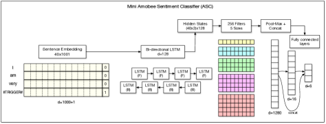
Figure 1: Architecture of the mini Amobee sentiment classifier.

1. The input was the official dataset, transformed using our trained embeddings, where the trigger word was embedded as an unknown word using the rare-words token. We concatenated an additional bit to each word vector, denoting whether it is the missing trigger-word, differentiating it from other unknown words. There are three key differences from our original work:

1. The GRU layer was replaced by an LSTM layer.

2. Residual connections were added from the output of the max-pooling layer to the network output.

3. Hyper parameters values were in the following ranges: embedding size=1000, LSTM hidden size=[128, 512], number of filters=[128, 512] and dense layer size=[16, 32].

Training a single mini-ASC module on the IEST 2018 training set using the Adam optimizer (Kingma and Ba, 2014), categorial cross entropy loss function and a batch size of 32, results in an average accuracy of $0.669$ on the official validation set.

6.2 First Ensemble

The first level ensemble incorporates 4 mini ASC modules and 3 identical sub-networks (see figure 2). The sub-networks share the same architecture and their inputs are the following:

1. Universal + DeepMoji embeddings; this network reaches an average F₁ score of 0.587 by itself on the validation set.

2. The LM1 + LM2 predictions; this network reaches an average F₁ score of 0.637 by itself on the validation set.

3. The Semeval 2018 predictions, together with the LM1 predictions; this network reaches an average F₁ score of 0.646 by itself on the validation set.

These networks share the same structure: the input is connected to a dense layer of dimension 16 and then concatenated with the input going into a final dense layer of size 6 with a softmax activation function. Dropout layers of $0.5$ are applied after the input and before the output layers.

The other 4 models are copies of the architecture described in 6.1. All orange layers of size 6 are outputs of the model and are trained against the labels with equal contribution to the total loss. We used the Adam optimizer with a batch size of 32, a learning rate of $5\cdot 10^{-4}$ and a decay of $5\cdot 10^{-5}$ (decay in Adam is introduced in Keras, and is not part of the original algorithm; it represents decay between batches). This network reaches an average F₁ score of $0.700$ on the validation set. This first ensemble is denoted by E1.

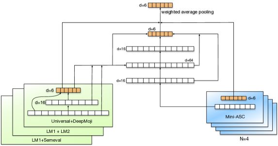
Figure 2: Architecture of the first-level ensemble.

6.3 Second Ensemble

In the second level ensemble (figure

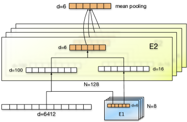
Figure 3: Architecture of the second-level ensemble.

3), we started with 8 copies of the aforementioned E1 models (with different parameters for the Mini ASC modules in the ranges described in section 6.1) and combined them with a concatenation of the following features (described in section 5): two external embeddings (Universal Sentence Embedding, DeepMoji) and our Semeval 2018 pipeline predictions.

We have used a dense layer of size 16 over the outputs of the 8 E1 models and a dense layer of size 100 over all of the above features (including the E1 outputs). These two layers were concatenated into a softmax layer of size 6 which was the output of the second ensemble; we denote this by E2. This E2 network reaches an average F₁ score of 0.702 on the validation set. The final model is a soft voting ensemble, comprising 128 networks of type E2; this probability averaging is meant to decrease the variance of the model which reaches an average F₁ score of 0.705 on the validation set.

Since the final model is an ensemble, where some models are somewhat overfitted with respect to the training dataset (e.g. E1) and some models are not overfitted at all (LM1), we decided to use the validation dataset to train the final model for an additional 4 epochs using a large batch size of 900. After this procedure, the system scored an F₁ of 0.7145 on the test dataset.

7 Review and Conclusions

In this paper we described the system developed for the WASSA 2018 implicit emotion shared task. It consists of a multi-level ensemble, combining a novel use of language models to predict the right emotion word, together with previous high-ranking architecture, used in the Semeval 2018 sentiment shared task, and two external embeddings. The system reached 1st place with macro F₁ of 0.7145, with the next system scoring 0.7105. Examining the nature of the this task, it is a combination of both sentiment classification and word prediction; this was the motivation of using the Semeval 2018 models, which were designed to classify emotions. On the other hand, the language model is specifically trained to maximize the likelihood of matching a word to a given sentence, thus naturally lending itself to the word prediction aspect of the task.

We have seen that splitting the dataset into two parts, one for training our models and the other for the ensembling process (in this case the second part is the validation set) is much more beneficial than training our models on the combined bigger dataset, in cases when some of the models are expected to be much less generalizable than others.

It is interesting to note the task organizers have tested human performance on a subset sample, achieving macro F₁ of 0.45, which is much lower than the automated systems.

We released the word embeddings and language model as open-source in order to benefit further research and increase sharing of resources.

Appendix A Emotions Lexicon

Emotion	Words
Anger	Anger, angry, fuming, angrily, angrier, angers, angered, furious.
Disgust	Disgust, disgusted, disgusting, disgustedly, disgusts.
Fear	Fear, feared, fearing, fearfully, frightens, fearful, afraid, scared.
Joy	Joy, happy, thrilling, joyfully, happily, happier, delights, joyful, joyous.
Sad	Sad, sadden, depressing, depressingly, sadder, depresses, sorrowful, saddened.
Surprise	Surprise, surprised, surprising, surprisingly, surprises, shocked.

Table 3: Emotion lexicon used to produce predictions using the language models.

References

- Abadi et al. (2016) Martín Abadi, Paul Barham, Jianmin Chen, Zhifeng Chen, Andy Davis, Jeffrey Dean, Matthieu Devin, Sanjay Ghemawat, Geoffrey Irving, Michael Isard, et al. 2016. Tensorflow: A system for large-scale machine learning. In OSDI, volume 16, pages 265–283.
- Bojanowski et al. (2017) Piotr Bojanowski, Edouard Grave, Armand Joulin, and Tomas Mikolov. 2017. Enriching word vectors with subword information. Transactions of the Association for Computational Linguistics, 5:135–146.
- Cer et al. (2018) Daniel Cer, Yinfei Yang, Sheng-yi Kong, Nan Hua, Nicole Limtiaco, Rhomni St. John, Noah Constant, Mario Guajardo-Cespedes, Steve Yuan, Chris Tar, Yun-Hsuan Sung, Brian Strope, and Ray Kurzweil. 2018. Universal sentence encoder. CoRR, abs/1803.11175.
- Chollet et al. (2015) François Chollet et al. 2015. Keras. https://github.com/keras-team/keras.
- Felbo et al. (2017) Bjarke Felbo, Alan Mislove, Anders Søgaard, Iyad Rahwan, and Sune Lehmann. 2017. Using millions of emoji occurrences to learn any-domain representations for detecting sentiment, emotion and sarcasm. In Conference on Empirical Methods in Natural Language Processing (EMNLP).
- Kingma and Ba (2014) Diederik P Kingma and Jimmy Ba. 2014. Adam: A method for stochastic optimization. arXiv preprint arXiv:1412.6980.
- Klinger et al. (2018) Roman Klinger, Orphée de Clercq, Saif M. Mohammad, and Alexandra Balahur. 2018. Iest: Wassa-2018 implicit emotions shared task. In Proceedings of the 9th Workshop on Computational Approaches to Subjectivity, Sentiment and Social Media Analysis, Brussels, Belgium. Association for Computational Linguistics.
- Mikolov et al. (2013) Tomas Mikolov, Ilya Sutskever, Kai Chen, Greg S Corrado, and Jeff Dean. 2013. Distributed representations of words and phrases and their compositionality. In C. J. C. Burges, L. Bottou, M. Welling, Z. Ghahramani, and K. Q. Weinberger, editors, Advances in Neural Information Processing Systems 26, pages 3111–3119. Curran Associates, Inc.
- Mohammad et al. (2018) Saif M. Mohammad, Felipe Bravo-Marquez, Mohammad Salameh, and Svetlana Kiritchenko. 2018. Semeval-2018 Task 1: Affect in tweets. In Proceedings of International Workshop on Semantic Evaluation (SemEval-2018), New Orleans, LA, USA.
- Řehůřek and Sojka (2010) Radim Řehůřek and Petr Sojka. 2010. Software Framework for Topic Modelling with Large Corpora. In Proceedings of the LREC 2010 Workshop on New Challenges for NLP Frameworks, pages 45–50, Valletta, Malta. ELRA. http://is.muni.cz/publication/884893/en.
- Rozental and Fleischer (2018) Alon Rozental and Daniel Fleischer. 2018. Amobee at semeval-2018 task 1: GRU neural network with a CNN attention mechanism for sentiment classification. CoRR, abs/1804.04380.
- Srivastava et al. (2014) Nitish Srivastava, Geoffrey Hinton, Alex Krizhevsky, Ilya Sutskever, and Ruslan Salakhutdinov. 2014. Dropout: a simple way to prevent neural networks from overfitting. The Journal of Machine Learning Research, 15(1):1929–1958.
- Vaswani et al. (2018) Ashish Vaswani, Samy Bengio, Eugene Brevdo, Francois Chollet, Aidan N. Gomez, Stephan Gouws, Llion Jones, Łukasz Kaiser, Nal Kalchbrenner, Niki Parmar, Ryan Sepassi, Noam Shazeer, and Jakob Uszkoreit. 2018. Tensor2tensor for neural machine translation. CoRR, abs/1803.07416.
- Vaswani et al. (2017) Ashish Vaswani, Noam Shazeer, Niki Parmar, Jakob Uszkoreit, Llion Jones, Aidan N. Gomez, Lukasz Kaiser, and Illia Polosukhin. 2017. Attention is all you need. CoRR, abs/1706.03762.