Abstract

In this paper, we adopt results in nonlinear time series analysis for causal inference in dynamical settings. Our motivation is policy analysis with panel data, particularly through the use of “synthetic control” methods. These methods regress pre-intervention outcomes of the treated unit to outcomes from a pool of control units, and then use the fitted regression model to estimate causal effects post-intervention. In this setting, we propose to screen out control units that have a weak dynamical relationship to the treated unit. In simulations, we show that this method can mitigate bias from “cherry-picking” of control units, which is usually an important concern. We illustrate on real-world applications, including the tobacco legislation example of Abadie et al., (2010), and Brexit.

1 Introduction

In causal inference, we compare outcomes of units who received the treatment with outcomes from units who did not. A key assumption, often made implicitly, is that the relationships of interest are static and invariant. For example, in studying the effects of schooling on later earnings, we usually consider potential outcomes $Y_{i}(k)$, for some student $i$ had the student received $k$ years of schooling. Since only one potential outcome can be observed for each student, causal inference needs to rely on comparisons between students who received varying years of schooling. The validity of the results therefore rests upon the assumption that the relationship between years of schooling and earnings is temporally static and unidirectional.

However, in many real-world settings, different variables exhibit dynamic interdependence, sometimes showing positive correlation and sometimes negative. Such ephemeral correlations can be illustrated with a popular dynamical system shown in Figure 1, the Lorenz system (Lorenz,, 1963). The trajectory resembles a butterfly shape indicating varying correlations at different times: in one wing of the shape, variables $X$ and $Y$ appear to be positively correlated, and in the other they are negatively correlated. Such dynamics present new methodological challenges for causal inference that have not been addressed. In relation to the schooling example, our analysis of schooling effect on earnings could occur on one wing of the system, where the correlation is, say, positive. However, crucial policy decisions, such as college subsidies, could occur on the other wing where the relationship is reversed. Such discord between data analysis and policy making is clearly detrimental to policy effectiveness.

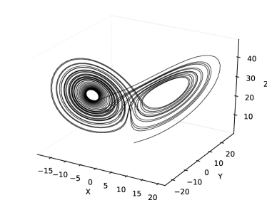
Figure 1: A Lorenz attractor plotted in 3D.

Despite its longstanding importance in many scientific fields, dynamical systems theory has not found a way into modern causal inference (Durlauf,, 2005). The main goal of this paper is to leverage key results from dynamical systems to guide causal inference in the presence of dynamics. For concreteness, we focus on synthetic control methods (Abadie et al.,, 2010), which are popular for policy analysis with panel data. Our methods, however, can more generally be applied when causal inference involves some form of matching between treated and control units in the time domain.

2 Preliminaries

Here, we give a brief overview of comparative case studies with panel data to fix concepts and notation. Later, in Section 3, we describe our method.

Following standard notation, we consider $J+1$ units, with only one unit being treated. Let $Y_{it}^{N}$ be the potential outcome for unit $i$ at time $t$ in a hypothetical world where the intervention did not occur (denoted by the exponent “N”), where $i=1,2,\ldots,J+1$, and $t=1,2,\ldots,T$; also let $Y_{it}^{I}$ be the corresponding potential outcome assuming the intervention did occur. Let $D_{it}$ be a binary indicator of whether unit $i$ is treated at time $t$. By convention, and without loss of generality, only unit 1 receives the treatment, and there exists $T_{0}\in(0,T)$ such that

$$D_{it}=1,~{}\text{if and only if}~{}i=1~{}\text{and}~{}t>T_{0}.$$

The observed outcome for unit $i$ at time $t$, denoted by $Y_{it}$, therefore satisfies:

$$Y_{it}=Y_{it}^{N}+(Y_{it}^{I}-Y_{it}^{N})D_{it},$$ (1)

where $\tau_{it}=Y_{it}^{I}-Y_{it}^{N}$ is the causal effect of intervention on unit $i$ at time $t$. Suppose there exist weights $w_{2},\ldots,w_{J+1}$ such that $\sum_{j=2}^{J+1}w_{j}=1$ and $w_{j}\geq 0$, and $Y_{1t}^{N}=\sum_{j=2}^{J+1}w_{j}Y_{jt}$, for $t=1,\ldots,T_{0}$. Then, the causal effect of the intervention can be estimated through:

$$\hat{\tau}_{1t}=Y_{1t}-\sum_{j=2}^{J+1}w_{j}Y_{jt},~{}\text{for every}~{}t>T_{0}.$$ (2)

The time series defined with the term $\sum_{j=2}^{J+1}w_{j}Y_{jt}$ in Equation (2) is the synthetic control. This synthetic control unit can be construed to be representative of the treated unit ($i=1$) had the treated unit not received treatment. Because of the constraints put on $w_{j}$, namely that they are nonnegative and sum to one, the fitted values of the weights reside on the edges of a polytope, and so many weights are set to 0. Such sparsity in the weights corresponds to control selection, and so only a few control units are used to model the outcomes of the treated unit.

The synthetic control methodology is an important example of comparative case studies (Angrist and Pischke,, 2008; Card and Krueger,, 1994), and generalizes other well-known methods, such as “difference-in-differences”. As a methodology it is simple and transparent, and so synthetic controls have become widely popular in the fields of policy analysis (Abadie et al.,, 2010; Kreif et al.,, 2016; Shaikh and Toulis,, 2019), criminology (Saunders et al.,, 2015), politics (Abadie and Gardeazabal,, 2003; Abadie et al.,, 2015), and economics (Billmeier and Nannicini,, 2013).

Theoretically, the treatment effect estimator, $\hat{\tau}_{1t}$, is asymptotically unbiased as the number of pre-intervention periods grows when the outcome model is linear in (possibly unobserved) factors and the treated unit “lives” in the convex hull of the controls (Abadie et al.,, 2010, Theorem 1). As such, a key assumption of model continuity is implicitly made for identification, where the weights $w_{j}$ are assumed to be time-invariant. Furthermore, control selection in synthetic controls depends only on the statistical fit between treated and control outcomes in the pre-intervention period, which opens up the possibility of cherry-picking controls to bias causal inference. In the following section, we illustrate these problems with an example.

2.1 Motivation: an Adversarial Attack to the Synthetic Control Method

As a motivation, we use the example of California’s tobacco control program in 1989, as described in the original paper of synthetic controls (Abadie et al.,, 2010). The goal is to estimate the effect of Proposition 99, a large-scale tobacco control program passed by electorate majority in 1988 in California. The proposition took effect in 1989 through a sizeable tax hike per cigarette packet. The panel data include annual state per-capita cigarette sales from 1970 to 2000 as outcome, along with related predictors, such as state median income and %youth population. We have a pool with 38 states as potential controls, after discarding states that adopted similar programs during the 1980’s.

The synthetic control methodology proceeds by calculating a weighted combination of control unit outcomes to fit cigarette sales of California, using only pre-1989 data. In this application, the weighted combination is: Colorado (0.164), Connecticut (0.069), Montana (0.199), Nevada (0.234), and Utah (0.334), where the numbers in the parentheses are the corresponding weights. The implied model is the following:

$$\widehat{Y}_{\mathrm{CA},t} =0.164\times Y_{\mathrm{CO},t}+0.069\times Y_{\mathrm{CT},t}$$ (3)

$$+0.199\times Y_{\mathrm{MO},t}+0.234\times Y_{\mathrm{NV},t}+0.334\times Y_{\mathrm{UT},t},$$

where $Y$ denotes packet sales at a particular state and time (a state is denoted by a two-letter code; e.g., $\mathrm{CA}$ stands for California). We note that time $t$ in the model of Equation (3) is before intervention ($t\leq 1989$), so that all states in the data, including California, are in control for the entire period considered in the model.

The idea for causal inference through this approach is that the same model in Equation (3) can be used to estimate the counterfactual outcomes for California, $Y_{\mathrm{CA},t}$, for $t>1989$, had California not been treated with the tax hike in 1989. By comparing the post-intervention data from actual California that was treated with the tobacco control program in 1989, and predictions for synthetic California that hypothetically stayed in control in 1989, we can estimate that per-capita cigarette sales reduced by 19 packs on average by Proposition 99, suggesting a positive causal effect. This is illustrated in the left figure of Figure 2. As mentioned earlier, an implicit assumption here is that of model continuity: we assume that the same model that fits pre-intervention California can be used to predict the counterfactual outcomes of a post-intervention, non-treated California.

This model continuity assumption relies critically on the choice of control units in the model of Equation (3). Currently, this choice relies mostly on the subject-matter expert, which leaves open opportunities for cherry-picking in constructing the control pool. To illustrate this problem we can perform the following manipulation. First, we add 9 unemployment-related time series, namely $Y^{\prime}_{\mathrm{AD1},t},\ldots,Y^{\prime}_{\mathrm{AD9},t}$, into the pool of potential controls, where “$\mathrm{AD}$” stands for “adversarial”. Second, before adding these units to the control pool we transform the time series as follows: $Y_{\mathrm{AD}i,t}=Y^{\prime}_{\mathrm{AD}i,t}-50+90\cdot\mathbb{I}\{t\leq 1989\}$. This transformation ensures that the adversarial time series has similar scale to time series on cigarette consumption before treatment. Since the synthetic control method only relies on statistical fit, it may pick up the artificial time series from the new control pool. Indeed, the new synthetic California is now described by the following model:

$$\widehat{Y}_{\mathrm{CA},t} =0.247\times Y_{\mathrm{CO},t}+0.179\times Y_{\mathrm{CT},t}$$ (4)

$$+0.196\times Y_{\mathrm{NV},t}+0.06\times Y_{\mathrm{NH},t}+0.011\times Y_{\mathrm{WY},t}$$

$$+0.3\times Y_{\mathrm{AD}\ast,t},$$

where $Y_{\mathrm{AD}\ast,t}$ represents that the adversarial time series was selected — the specific index is irrelevant. This produces a new synthetic California that is drastically different than before. The weight on the artificial control unit is in fact the highest compared to the weights on all other units, which is clearly undesirable. More importantly, with the new synthetic control California, we estimate a negative causal effect of 8 packs on average (see right sub-figure in Figure 2).

Figure 2: Trends in per-capita cigarette sales. The solid line is actual California and the dashed line is synthetic California, while the vertical line indicates time of intervention. Left: original setting. Right: adversarial setting where the synthetic California is created according to Equation (4).

To address this problem, our paper leverages fundamental results in dynamical systems theory, such as time-delay embeddings. The goal is to pre-screen control units based on how strongly related they are to treated units from a dynamical point of view. The key idea is that state cigarette consumption data evolve on the same attractor, whereas adversarial time series do not. Thus, the latter should be less dynamically related to the treated state, and so they should be removed from the control pool.

We note that our proposed method differs from recent work in synthetic controls, which has mainly focused on high-dimensional, matrix completion, or de-biasing methods (Amjad et al.,, 2018; Ben-Michael et al.,, 2018; Athey et al.,, 2018; Hazlett and Xu,, 2018). These methods take a regression model-based approach, whereas we treat panel data as a nonlinear dynamical system. More broadly, our approach shows that dynamical systems theory can be integrated into statistical frameworks of causal inference, a goal that so far has remained elusive (Rosser,, 1999; Durlauf,, 2005).

3 Methods

In this section, we describe our proposed method. In Section 3.1, we present the method of convergent cross mapping (CCM), which is the fundamental building block of our method. In Section 3.2, we motivate CCM through a theoretical analysis on a simple, non-trivial time-series model. Finally, in Section 3.3, we give details on our proposed method.

3.1 Convergent Cross Mapping (CCM)

The basis of our approach is to consider the available panel data as a dynamical system. In particular, the state of the system at time $t$ is the collection of all time series, $(Y_{1t},Y_{2t},\ldots,Y_{(J+1)t})$, where $J$ is the number of controls. Taken across all possible $t$, this implies a manifold, known as the phase space, denoted by $M=\left\{(Y_{jt}:j\in 1,\ldots,J+1):t\in[0,T]\right\}$, where $T$ denotes the length of time series, and is fixed. For example, when $J=1$ there are two units in total and $M$ is a curve (possibly self-intersecting) on the plane.

A seminal result in nonlinear dynamics is Takens’ theorem (Takens,, 1981), which shows that the phase space of a dynamical system can be reconstructed through time-delayed observations from the system. Specifically, let us define a delay-coordinate embedding of the form

$$\widetilde{Y}_{jt}=[Y_{jt},Y_{j(t-\tau)},\ldots,Y_{j(t-(d-1)\tau)}],$$ (5)

where $\tau>0$ is the time delay. The key theoretical result of Takens, (1981) is that the manifold, $\widetilde{M}_{j}$, defined from outcomes $\{\widetilde{Y}_{jt}\}$ is diffeomorphic (i.e., the mapping is differentiable, invertible, and smooth) to the original manifold $M$, meaning that some important topological information is preserved, such as invariance to coordinate changes. In other words, $\widetilde{M}_{j}$ is a reconstruction of $M$. It follows that different reconstructions $\widetilde{M}_{j}$, for various $j$, are diffeomorphic to each other, including the original manifold $M$, which implies cross-predictability. For two different reconstructions $\widetilde{M}_{j}$ and $\widetilde{M}_{j^{\prime}}$, with their corresponding base time series $Y_{jt}$ and $Y_{j^{\prime}t}$, we could use $\widetilde{M}_{j}$ to predict $Y_{j^{\prime}t}$ and use $\widetilde{M}_{j^{\prime}}$ to predict $Y_{j}$. By measuring this cross-predictability, the relative strength of dynamical relationship between any two variables in the system can be quantified (Schiff et al.,, 1996; Arnhold et al.,, 1999).

One recent method utilizing this idea is convergent cross mapping (Sugihara et al.,, 2012, CCM). In addition to the idea of cross-predictability, CCM also relies on a smoothness implication of Takens’ theorem, whereby neighboring points in the reconstructed manifold are close to neighboring points in the original manifold. This suggests that cross predictability will increase and stabilize as the number of data points grow. The cross predictability is quantified by a CCM score, which we will address later.

Operationally, the generic CCM algorithm considers two time series, say $X_{t}$ and $Y_{t}$, and their corresponding delay-coordinate embedding vectors at time $t$, namely

$$\widetilde{X}_{t}=[X_{t},X_{(t-\tau)},\ldots,X_{(t-d\tau+\tau)}],$$ (6)

$$\widetilde{Y}_{t}=[Y_{t},Y_{(t-\tau)},\ldots,Y_{(t-d\tau+\tau)}],$$

where $d$ is known as the embedding dimension and $t\in\{1+(d-1)\tau,1+d\tau,\ldots,T\}$. The manifold based on the phase space of $\widetilde{Y}_{t}$ is denoted by $M_{Y}$, and the manifold based on $\widetilde{X}_{t}$ is denoted by $M_{X}$, where the manifold definitions follow from Equation (5). The idea is that these manifolds are diffeomorphic to the original manifold of the dynamical system of $Y$ and $X$. A manifold from the delay embedding of one variable can be used to predict the other variable, and the quality of this prediction is an indication of which variable “drives” the other.

Such prediction proceeds in discrete steps as follows. First, we build a nonparametric model of $X_{t}$ using the reconstruction manifold based on $Y_{t}$. For a given time point $t$ we pick the $(d+1)$-nearest neighbors from $t\in\{1+(d-1)\tau,1+d\tau,\ldots,L\}$ in $\widetilde{Y}_{t}$, where $L<T$ is called the library size, and denote their time indices (from closest to farthest) as $\{t_{1},\cdots,t_{d+1}\}$. A linear model for $X_{t}$ is as follows:

$$\widehat{X}_{t}=\sum\nolimits_{i=1}^{d+1}w(t_{i},t)X_{t_{i}},$$ (7)

where $w(t_{i},t)$ is the weight based on the Euclidean distance between $\widetilde{Y}_{t}$ and its $i$-th nearest neighbor on $\widetilde{Y}_{t_{i}}$, for example, $w(t_{i},t)=\exp(-d_{i}/d_{1})/\sum_{j}\exp(-d_{j}/d_{1})$ and $d_{i}=||\widetilde{Y}_{t}-\widetilde{Y}_{t_{i}}||$, with the usual $L_{2}$ norm. The difference defined by mean absolute error (MAE) between $X_{t}$ and $\widehat{X}_{t}$ across $t$ is defined as the CCM score of $Y_{t}$ on $X_{t}$ (lower is better):

$$\mathrm{CCM}(X_{t}\mid Y_{t})=|X_{t}-\widehat{X}_{t}|,$$ (8)

$$\mathrm{CCM}(Y_{t}\mid X_{t})=|Y_{t}-\widehat{Y}_{t}|.$$

Intuitively, the CCM score captures how much information is in $Y_{t}$ about $X_{t}$. For instance, if $X_{t}$ dynamically drives $Y_{t}$ we expect $\widehat{X}_{t}$ to be close to $X_{t}$. Similarly, $\mathrm{CCM}(Y_{t}\mid X_{t})$ is obtained by repeating the above procedure symmetrically, using $M_{X}$ of the values from the delay embedding $\widetilde{X}_{t}$ of $X_{t}$. The value of $\mathrm{CCM}(Y_{t}\mid X_{t})$ quantifies the information in $X_{t}$ about $Y_{t}$. The two CCM scores jointly quantify the dynamic coupling between the two variables. As mentioned earlier, Takens’ theorem implies that there exists a one-to-one mapping such that the nearest neighbors of $Y_{t}$ identify the corresponding time indices of nearest neighbors of $X_{t}$, if $X_{t}$ and $Y_{t}$ are dynamically related. As the library size, $L$, increases, the reconstruction manifolds $M_{X}$ and $M_{Y}$ become denser and the distances between the nearest neighbors shrink, and so the CCM scores will converge; see Sugihara and May, (1990); Casdagli et al., (1991) for more details.

From a statistical perspective, the CCM method is a form of nonparametric time-series estimation (Härdle et al.,, 1997). The unique feature of CCM, and more generally of delay embedding methods, is that the nonparametric components are in fact the time indices $t_{1},\ldots,t_{d+1}$ in Equation (7). This differs from, say, kernel smoothing (Hastie et al.,, 2001), where the target point $X_{t}$ is fitted by neighboring observations to smooth estimation. Importantly, CCM is not in competition with Granger causality (Granger,, 1969), but rather complements it. The key problem with Granger causality is that it requires “separability” of the effects from different causal factors. This condition generally does not hold in real-world dynamical systems that exhibit so called “weak coupling”. CCM is unique because it can work in such systems (Sugihara et al.,, 2012). Finally, CCM is backed up by a growing literature in the physical sciences as it is tailored to dynamical complex systems (Runge et al.,, 2019).

3.2 Theory of CCM on Autoregressive Model

In this section, we illustrate CCM through an AR(1) autoregression model. Of course, AR(1) is a simple model that most certainly does not capture the details of real-world time series. However, its simplicity allows us to do two things. First, we derive analytic formulas for the CCM scores in Equation (8). Due to CCM’s nonlinear nature, such formulas are not easily attainable, in general. In fact, we are unaware of any other analytic expressions for CCM in the literature, so our work here makes a broader contribution. Second, we can compare the CCM formulas with the parameters of the AR(1) model to better understand CCM as a tool; this is only possible because AR(1) is simple enough that the strength of causal relationships between variables is discernible from the model parameters.

The outcome model we consider is as follows:

$$X_{t}=\alpha X_{t-1}+\mu+\epsilon_{t},\quad\quad Y_{t}=\beta X_{t-1}+\mu+\zeta_{t},$$ (9)

where $\alpha$, $\beta$ are fixed, with $|\alpha|<1$, $\beta\geq 0$, $\mu$ is the drift, $\epsilon_{t}\sim N(0,\sigma_{X}^{2})$ and $\zeta_{t}\sim N(0,\sigma_{Y}^{2})$ are zero-mean and constant-variance normal errors, with $\sigma_{Y}>\sigma_{X}$. In this joint dynamical system of $X$ and $Y$, it is evident that $X$ generally drives $Y$ since $X$ evolves independently of $Y$, whereas the evolution of $Y$ depends on $X$. We are interested in knowing how CCM quantifies this asymmetric dynamic relationship between $X$ and $Y$, and whether it captures the dependence on parameters $\alpha,\beta,\mu,\sigma_{X}^{2},\sigma_{Y}^{2}$.

Assumption 1.

Fix $t$ and let $L\to\infty$. Suppose that:

1. $\min_{i=1,\ldots,d+1}\min\{t_{i}^{\prime},t_{i}\}\to\infty$;

2. for both crossmaps, $\max_{i}|w_{Y}(t_{i},t)-\frac{1}{d+1}|\to 0$, and $\max_{i}|w_{X}(t_{i}^{\prime},t)-\frac{1}{d+1}|\to 0$;

3. $\min_{i\neq j}{|t_{i}-t_{j}|}\to\infty$ and $\min_{i\neq j}{|t_{i}^{\prime}-t_{j}^{\prime}|}\to\infty$.

Remarks. Assumption 1(a) requires some form of smoothness for the delay-coordinate system, and is mild. Assumption 1(b) is similar to stationarity as it implies exchangeability within the sets $\{t_{i}:i=1,\ldots,d+1\}$ and $\{t_{i}^{\prime}:i=1,\ldots,d+1\}$. Assumption 1(c) may be strict. It could fail, for instance, when the order statistics (e.g., $\{\widetilde{Y}_{t_{i}}\}$) are periodic.

Theorem 1.

Suppose that Assumptions 1(a)-(c) hold for the CCM scores of the autoregressive model in Equation (9), then

$$\mathrm{CCM}(X_{t}\mid Y_{t}) \xrightarrow{\text{d}}\mathrm{FN}\bigg{(}(X_{0}-\frac{\mu}{1-\alpha})\alpha^{t},\frac{2-\alpha^{2t}}{1-\alpha^{2}}\sigma_{X}^{2}\bigg{)},$$

$$\mathrm{CCM}(Y_{t}\mid X_{t}) \xrightarrow{\text{d}}\mathrm{FN}\bigg{(}\beta(X_{0}-\frac{\mu}{1-\alpha})\alpha^{t-1},$$

$$\frac{2-\alpha^{2t}}{1-\alpha^{2}}\beta^{2}\sigma_{X}^{2}+2\sigma_{Y}^{2}\bigg{)},$$

where $\mathrm{FN}(\mu,\sigma^{2})=|N(\mu,\sigma^{2})|$ is the folded normal distribution with mean $\mu$ and variance $\sigma^{2}$.

Remarks. To unpack this theoretical result, we make the following remarks:

1. When $\beta=0$, the dependence of $Y_{t}$ on $X_{t}$ is entirely lost, and so $X_{t}$ and $Y_{t}$ evolve independently implying that there is no driving factor in the system. CCM captures this relationship, since $\mathrm{CCM}(X_{t}\mid Y_{t})=O_{P}(\sigma_{X})$ and $\mathrm{CCM}(Y_{t}\mid X_{t})=O_{P}(\sigma_{Y})$, with the two scores being independent (this is shown in the proof of the theorem in the Supplement).

2. When $\beta$ is small or moderately large, $Y_{t}$ is weakly dependent on $X_{t}$. On average, we expect to see that $\mathrm{CCM}(Y_{t}\mid X_{t})>\mathrm{CCM}(X_{t}\mid Y_{t})$. CCM analysis indicates correctly that the driving factor in the system is $X_{t}$ and not $Y_{t}$ (recall that we are using the absolute error-CCM, and so smaller values are better).

3. When $\beta$ is very large we could sometimes have $\mathrm{CCM}(Y_{t}\mid X_{t})<\mathrm{CCM}(X_{t}\mid Y_{t})$, which leads to the wrong “causal direction”. This shows some inherent limitations of CCM, as it depends to some extent on predictive ability, and so it can fail in similar ways as Granger causality.

In conclusion, Theorem 1 is a new connection of statistics and nonlinear dynamics. As mentioned earlier, the goal is not to analyze AR(1) per se, which indeed is a simple model, but to understand CCM’s causal predictions by comparing to AR(1) coefficients. The theorem explains how and why CCM is capturing the directions correctly, and justifies using CCM in synthetic controls. A similar analysis of CCM in more complex models would be desirable, but is generally hard since CCM is highly nonlinear. We leave this for future work.

3.3 CCM+SCM Method and Proposition 99

Here, we present CCM scores in the Proposition 99 example introduced in Section 2.1. Specifically, California (CA) is cross-mapped with five control states selected by the standard synthetic control method as shown in Equation (3). We use per-capita cigarette sales from the pre-intervention period as the outcome variable, which gives 19 data points for each unit’s time-series. The cross predictability measured by the CCM scores for each pair is shown in Figure 3. For example, the California-Colorado pair includes two CCM curves, namely, $\mathrm{CCM}(Y_{\mathrm{CA},t}\mid Y_{\mathrm{CO},t})$ and $\mathrm{CCM}(Y_{\mathrm{CO},t}\mid Y_{\mathrm{CA},t})$.

We see that cross predictability for all pairs roughly converge as the library size, $L$, grows. Furthermore, most pairs converge to the same low level of CCM score, indicating a strong and bidirectional dynamical relationship between the state pairs. The only obvious exception is the California-Connecticut pair, where a big gap occurs between the two curves exists, indicating a weak dynamical relationship between them.

In particular, we see that Connecticut is better predicted from California than the other way round. For this reason, we argue that Connecticut is not a suitable control for California and should be removed from the donor pool. If we apply an averaging transformation to smooth out the 1970-1980 trend of Connecticut, the CCM score changes and now shows a strong dynamic coupling between the two states (bottom-right plot in Figure 3). If Connecticut is removed, SCM will pick Minnesota. However, CCM will screen Minnesota as well because the cigarette price trends are similar between Minnesota and Connecticut, but distinct from California.

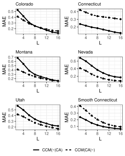
Figure 3: CCM scores based on MAE between California and control states with varying library size $L$. $\mathrm{CCM}(CA\mid\sim)$ means cross predicting California from control, and $\mathrm{CCM}(\sim\mid CA)$ means cross predicting control from California.

Figure 4: Trends in per-capita cigarette sales after CCM pre-screening. The solid line is actual California and the dashed line is synthetic California, while the vertical line indicates time of intervention. Left: original setting. Right: adversarial setting where artificial units are added to the donor pool.

Our proposed method is therefore to use CCM to filter out controls that have a weak dynamical relationship with the treated unit, and then apply the standard SCM method as described in Section 2. We refer to this method as “CCM+SCM". In practice, we propose that CCM+SCM filters out a control unit if in the two CCM plots with the treated unit, either the minimum MAE or the MAE gap exceed some thresholds. To determine the cutoff values, we may use Monte-Carlo simulations where we add noise to the original series, and then estimate the null distribution of CCM values under a hypothesis of weak dynamical relationship.

To illustrate the potential of CCM+SCM, we return to the example of Section 2.1, where we showed that adversarial units in the control pool affected the performance of synthetic controls. Figure 4 shows that CCM+SCM is able to screen the adversarial units, and is able to produce a synthetic control that is indistinguishable from the non-adversarial setting. In the following section, we explore the performance of CCM+SCM further through simulated studies and real-world data.

4 Experiments and Applications

Here, we design adversarial settings where artificial units are added to the donor pool to bias the synthetic control method. Of particular interest is whether CCM+SCM can help filter out the artificial units in all cases, without affecting the baseline performance when artificial units are not present. We also consider real-world applications.

4.1 Simulations with Artificial Units

First, we expand the tobacco legislation example of Section 2.1 by introducing a larger set of artificial units, which are created adversarially. These artificial data were created based on real-world time series macroeconomic data. The detailed generation process can be found in the Supplement. We run simulation studies in which the true effect is known for the treated unit. We replace the true California with the following formula:

$$\widetilde{Y}_{\mathrm{CA},t} =0.164\times Y_{\mathrm{CO},t}+0.069\times Y_{\mathrm{CT},t}+0.199\times Y_{\mathrm{MO},t}$$

$$+0.234\times Y_{\mathrm{NV},t}+0.334\times Y_{\mathrm{UT},t}+\tau\mathbb{I}\{t\geq 1989\},$$

where $\tau$ is the true treatment effect and the other terms construct the synthetic California from the original data. This construction ensures that the ground truth of synthetic California in the post-intervention period is known. To illustrate that CCM is a general framework for pre-screening, we incorporate CCM to three different synthetic control methods: 1) SCM: vanilla synthetic control method by Abadie et al., (2010); 2) MC: matrix completion method for causal panel data by Athey et al., (2017); 3) RSC: robust synthetic control method by Amjad et al., (2018).

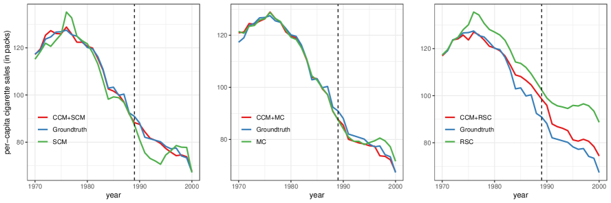
Figure 5: Comparisons of between ground truth and constructed synthetic California with and without CCM by three synthetic control methods. (In this simulation, $\tau=4$, but the results are robust to this value).

The comparisons between the ground truth and three synthetic control methods with and without CCM are visualized in Figure 5. The different methods lead to the same conclusion: with CCM pre-screening the outcome estimates, in both pre- and post-intervention periods, are closer to the ground truth than the original method alone. We note that MC works by matrix completion instead of selecting control units so CCM+MC behaves very similarly to MC. RSC alone does not work well because it uses the artificial unit to construct the synthetic control, and the denoising via singular value thresholding does not help here. The result suggests that CCM can help in synthetic control models, and is robust to the selection of the underlying outcome imputation model. Intuitively, this is because CCM is able to capture nonlinear dynamical information that is not captured by standard statistical models.

4.2 Real-World Applications

Here, we consider how many artificial units CCM is able to filter out with real-world data. To that end, we work with two real applications: one is still the California’s Tobacco Control Program studied in Abadie et al., (2010); and the other is on the economic costs of the Brexit referendum vote on UK’s GDP reported in Born et al., (2017). We only compare SCM and CCM+SCM. Our results are robust to the selection of the underlying model. As before, artificial units are created from noisy copies of real-world time series.

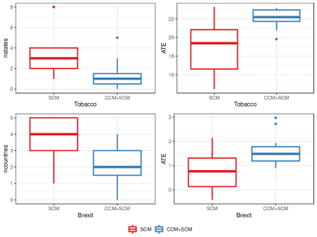
Figure 6: Box plots of the number of artificial control units selected by each method (left), namely SCM and CCM+SCM, and average treatment effect (right) in the Tobacco and Brexit applications.

Figure 6 shows the number of artificial units that are selected as controls, and the corresponding average treatment effect (ATE). Clearly, CCM+SCM selects much fewer artificial units than just SCM. In addition, CCM+SCM generates more stable estimates of ATE. Specifically, in the tobacco example, the ATE reported by CCM+SCM remains stable around 20, which is close to the original ATE ($\approx 19$ packets) estimated by SCM without artificial controls. In contrast, the ATE estimate from SCM with artificial controls is more varied in a range from 5 to 23. Another interesting phenomenon is that the ATE estimate from SCM can be negative under certain artificial controls in Brexit. This means that the effects of the Brexit vote may have been overstated in ongoing econometric work that uses synthetic control methods, as the estimates are likely to be sensitive to control pool construction.

5 Discussion

In this section, we discuss some general aspects of our work, particularly CCM as a causal inference method, and its underlying assumptions.

Our first point revolves around the use of CCM, and related dynamical systems methods, for causal inference. In particular, due to the success of CCM in quantifying dynamical relationships illustrated here, it may be tempting to consider CCM as a general method for causal inference (Sugihara et al.,, 2012; Deyle et al.,, 2013). However, we do not advocate doing that directly, for two main reasons. First, the statistical properties of methods such as CCM are not well known. Theorem 1 in this paper is a step to this direction, but more work is needed. Second, CCM does not account for the observation model (e.g., the treatment assignment mechanism), which is crucial in causal inference (Imbens and Rubin,, 2015). We also provide counterexamples and additional discussion in the Supplement.

Regarding the stationarity assumption in Theorem 1 (i.e., $|\alpha|<1$, and Assumption 1(b)), we note that CCM assumes a deterministic (possibly chaotic) system, and so stationarity is roughly mapped to “evolution on an attractor”. Stationarity in Theorem 1 is thus not directly applicable to Takens’ theorem, and is assumed only in our effort to understand CCM vis-à-vis AR(1). In this work, we argue that CCM can strengthen the model continuity assumption (pre- and post-treatment), which is left implicit in synthetic controls. But there is much left to understand about the connection between chaotic and stochastic systems (Casdagli,, 1992). We hope that this work provides a good motivation.

6 Conclusion

In this paper, we leveraged results from dynamical systems theory to quantify the strength of dynamic relationship between treated and control units in causal inference. We showed that this is useful in the context of comparative cases studies to guard against cherry-picking of potential controls, which is an important concern in practice.

More generally, our work opens up the potential for an interplay between dynamical systems theory and causal inference. In practice, interventions typically occur on complex dynamical systems, such as an auction or a labor market, which always evolve, before and after treatment. Future work could focus more on theoretical connections between embedding methods, such as CCM, and standard treatment effects in econometrics, especially if we view the filtering process described in Section 3 as a way to do treated-control matching.

References

- Abadie et al., (2010) Abadie, A., Diamond, A., and Hainmueller, J. (2010). Synthetic control methods for comparative case studies: Estimating the effect of california’s tobacco control program. Journal of the American Statistical Association, 105(490):493–505.
- Abadie et al., (2015) Abadie, A., Diamond, A., and Hainmueller, J. (2015). Comparative politics and the synthetic control method. American Journal of Political Science, 59(2):495–510.
- Abadie and Gardeazabal, (2003) Abadie, A. and Gardeazabal, J. (2003). The economic costs of conflict: A case study of the basque country. American Economic Review, 93(1):113–132.
- Amjad et al., (2018) Amjad, M., Shah, D., and Shen, D. (2018). Robust synthetic control. The Journal of Machine Learning Research, 19(1):802–852.
- Angrist and Pischke, (2008) Angrist, J. D. and Pischke, J.-S. (2008). Mostly Harmless Econometrics: An Empiricist’s Companion. Princeton University Press.
- Arnhold et al., (1999) Arnhold, J., Grassberger, P., Lehnertz, K., and Elger, C. E. (1999). A robust method for detecting interdependences: Application to intracranially recorded eeg. Phys. D, 134(4):419–430.
- Athey et al., (2017) Athey, S., Bayati, M., Doudchenko, N., Imbens, G., and Khosravi, K. (2017). Matrix completion methods for causal panel data models.
- Athey et al., (2018) Athey, S., Bayati, M., Doudchenko, N., Imbens, G., and Khosravi, K. (2018). Matrix completion methods for causal panel data models. Technical report, National Bureau of Economic Research.
- Ben-Michael et al., (2018) Ben-Michael, E., Feller, A., and Rothstein, J. (2018). The augmented synthetic control method. arXiv preprint arXiv:1811.04170.
- Billmeier and Nannicini, (2013) Billmeier, A. and Nannicini, T. (2013). Assessing economic liberalization episodes: A synthetic control approach. The Review of Economics and Statistics, 95(3):983–1001.
- Born et al., (2017) Born, B., Müller, G. J., Schularick, M., and Sedlacek, P. (2017). The Economic Consequences of the Brexit Vote. Discussion Papers 1738, Centre for Macroeconomics (CFM).
- Bureau of Labor Statistics, (2018) Bureau of Labor Statistics, U. D. o. L. (2018). Local Area Unemployment Statistics.
- Card and Krueger, (1994) Card, D. and Krueger, A. (1994). Minimum wages and employment: A case study of the fast-food industry in new jersey and pennsylvania. American Economic Review, 84(4):772–93.
- Casdagli, (1992) Casdagli, M. (1992). Chaos and deterministic versus stochastic non-linear modelling. Journal of the Royal Statistical Society: Series B (Methodological), 54(2):303–328.
- Casdagli et al., (1991) Casdagli, M., Eubank, S., Farmer, J. D., and Gibson, J. (1991). State space reconstruction in the presence of noise. Phys. D, 51(1-3):52–98.
- Deyle et al., (2013) Deyle, E. R., Fogarty, M., Hsieh, C.-h., Kaufman, L., MacCall, A. D., Munch, S. B., Perretti, C. T., Ye, H., and Sugihara, G. (2013). Predicting climate effects on pacific sardine. Proceedings of the National Academy of Sciences, 110(16):6430–6435.
- Durlauf, (2005) Durlauf, S. N. (2005). Complexity and empirical economics. The Economic Journal, 115(504):F225–F243.
- Granger, (1969) Granger, C. W. J. (1969). Investigating causal relations by econometric models and cross-spectral methods. Econometrica, 37(3):424–438.
- Härdle et al., (1997) Härdle, W., Lütkepohl, H., and Chen, R. (1997). A review of nonparametric time series analysis. International Statistical Review, 65(1):49–72.
- Hastie et al., (2001) Hastie, T., Tibshirani, R., and Friedman, J. (2001). The Elements of Statistical Learning. Springer.
- Hazlett and Xu, (2018) Hazlett, C. and Xu, Y. (2018). Trajectory balancing: A general reweighting approach to causal inference with time-series cross-sectional data.
- Imbens and Rubin, (2015) Imbens, G. W. and Rubin, D. B. (2015). Causal inference in statistics, social, and biomedical sciences. Cambridge University Press.
- Kreif et al., (2016) Kreif, N., Grieve, R., Hangartner, D., Turner, A. J., Nikolova, S., and Sutton, M. (2016). Examination of the synthetic control method for evaluating health policies with multiple treated units. Health Economics, 25(12):1514–1528.
- Lorenz, (1963) Lorenz, E. N. (1963). Deterministic nonperiodic flow. Journal of the Atmospheric Sciences, 20(2):130–141.
- Rosser, (1999) Rosser, J. B. (1999). On the complexities of complex economic dynamics. The Journal of Economic Perspectives, 13(4):169–192.
- Runge et al., (2019) Runge, J., Bathiany, S., Bollt, E., Camps-Valls, G., Coumou, D., Deyle, E., Glymour, C., Kretschmer, M., Mahecha, M. D., Muñoz-Marí, J., et al. (2019). Inferring causation from time series in earth system sciences. Nature communications, 10(1):1–13.
- Saunders et al., (2015) Saunders, J., Lundberg, R., Braga, A. A., Ridgeway, G., and Miles, J. (2015). A synthetic control approach to evaluating place-based crime interventions. Journal of Quantitative Criminology, 31(3):413–434.
- Schiff et al., (1996) Schiff, S. J., So, P., Chang, T., Burke, R. E., and Sauer, T. (1996). Detecting dynamical interdependence and generalized synchrony through mutual prediction in a neural ensemble. Phys. Rev. E, 54:6708–6724.
- Shaikh and Toulis, (2019) Shaikh, A. and Toulis, P. (2019). Randomization tests in observational studies with staggered adoption of treatment. University of Chicago, Becker Friedman Institute for Economics Working Paper, (2019-144).
- Sugihara et al., (2012) Sugihara, G., May, R., Ye, H., Hsieh, C.-h., Deyle, E., Fogarty, M., and Munch, S. (2012). Detecting causality in complex ecosystems. 338.
- Sugihara and May, (1990) Sugihara, G. and May, R. M. (1990). Nonlinear forecasting as a way of distinguishing chaos from measurement error in time series. Nature, 344(6268):734–741.
- Takens, (1981) Takens, F. (1981). Detecting strange attractors in turbulence. Lecture Notes in Mathematics, Berlin Springer Verlag, 898:366.