Transport in a thin topological insulator with potential and magnetic barriers

Abstract

We study transport across either a potential or a magnetic barrier which is placed on the top surface of a three-dimensional thin topological insulator (TI). For such thin TIs, the top and bottom surfaces interact via a coupling $\lambda$ which influences the transport properties of junctions constructed out of them. We find that for junctions hosting a potential barrier, the differential conductance oscillates with the barrier strength. The period of these oscillations doubles as the coupling $\lambda$ changes from small values to a value close to the energy of the incident electrons. In contrast, for junctions with a magnetic barrier, the conductance approaches a nonzero constant as the barrier strength is increased. This feature is in contrast to the case of transport across a single TI surface where the conductance approaches zero as the strength of a magnetic barrier is increased. We also study the spin currents for these two kinds of barriers; in both cases, the spin current is found to have opposite signs on the top and bottom surfaces. Thus this system can be used to split applied charge currents to spin currents with opposite spin orientations which can be collected by applying opposite spin-polarized leads to the two surfaces. We show that several of these features of transport across finite width barriers can be understood analytically by studying the $\delta$-function barrier limit. We discuss experiments which may test our theory.

I Introduction

Three-dimensional topological insulators have been extensively studied for the last several years both theoretically kane1 ; bern ; kane2 ; moore ; hasan1 ; qi2 and experimentally chen ; cheng ; hsieh1 ; hsieh2 ; xia ; roushan . A topological insulator (TI) is a material which is gapped in the bulk and has gapless states at all the surfaces which have a Dirac-type linear energy-momentum dispersion and are protected by time-reversal symmetry. Examples of such materials include Bi₂Se₃ and Bi₂Te₃. The bulk topological aspects of these TIs can be characterized by four integers $\nu_{0}$ and $\nu_{1,2,3}$ kane2 . The first integer $\nu_{0}$ classifies these TIs as strong ($\nu_{0}=1$) or weak ($\nu_{0}=0$), while the others, $\nu_{1,2,3}$, characterize the time-reversal invariant momenta at which the bulk Kramer pair bands cross: $\vec{L}_{0}=(\nu_{1}\vec{b}_{1},\nu_{2}\vec{b}_{2},\nu_{3}\vec{b}_{3})/2$, where $\vec{b}_{1,2,3}$ are the reciprocal lattice vectors. The strong topological insulators are robust against the presence of time-reversal invariant perturbations such as nonmagnetic disorder or lattice imperfections. It is well-known that kane2 ; qi2 ; hasan1 the surface of a strong TI has an odd number of Dirac cones. The positions of these cones are determined by the projection of $\vec{L}_{0}$ on to the surface Brillouin zone. The number of these cones depends on the nature of the surface; for example, for materials such as ${\rm HgTe}$ and ${\rm Bi_{2}Se_{3}}$, surfaces with a single Dirac cone at the center of the two-dimensional Brillouin zone have been found hasan1 ; hsieh1 ; hsieh2 .

The effective Dirac Hamiltonians governing the surface states can be derived starting from the bulk continuum Hamiltonian liu2 ; zhang3 ; deb1 . The surface states are known to exhibit spin-momentum locking in which the directions of spin angular momentum and linear momentum lie in the same plane and are perpendicular to each other hsieh4 . Several interesting properties of these surface Dirac electrons have been studied. These include proximity effects between an s-wave superconductor and the surface states and the consequent appearance of Majorana states fu2 . Various properties of junctions between different surfaces of TIs have been studied in Refs. deb2, ; wickles, ; biswas, ; alos, ; sitte, ; apalkov, ; habe, . Junctions of surfaces of a TI with normal metals, magnetic materials and superconductors have also been studied modak ; soori ; nuss . The effects of potential, magnetic and superconducting barriers on the surface of a TI have been studied in Refs. mondal, and peeters, . Spin-charge coupled transport on the surface of a TI has been studied in Ref. burkov, , leading to interesting magnetoresistance effects. Magnetic textures, such as domain walls and vortices, in a ferromagnetic thin film deposited on the surface of a TI have been examined in Ref. nomura, . The dynamics of magnetization coupled to the surface Dirac fermions has been investigated theoretically in Ref. yoko, . There have also been studies of transport in TI $p-n$ junctions in the presence of a magnetic field ilan ; dai , magnetotransport in patterned TI nanostructures moors , and the effects of disorder on transport zhou .

More recently, several theoretical studies have been carried out for thin films of a TI where the hybridization of the states on the opposite surfaces of the system shan gives rise to interesting phenomena. These phenomena include quantum phase transitions in the presence of a parallel magnetic field zyu and the appearance of a number of topological and nontopological phases asmar . It has been shown that a Coulomb interaction between the opposite surfaces can give rise to a topological exciton condensate serad1 , and a Zeeman field and a proximate superconductor can then give rise to Majorana edge modes serad2 . A number of other effects of finite width have been studied in Refs. shen, ; linder, ; egger, ; kundu, ; shenoy, ; pertsova, . However, the transport properties of such thin TIs in the presence of potential or magnetic barriers have not been studied before. Motivated by the above studies, we will consider in this paper a simple model of a TI with a coupling, characterized by a strength $\lambda$, between the top and the bottom surfaces; we will study the various features of electronic transport in such a system when a potential or magnetic barrier is applied on one of the surfaces.

The main results that arise out of our study can be summarized as follows. First, we show that for junctions with a potential barrier on the top surface, the tunneling conductance $G$ of the junctions oscillates with the barrier strength. The period of these oscillations can be tuned by changing $\lambda$; it doubles as $\lambda$ is increased from zero to a value close to the incident energy of the Dirac electrons on the surface. Second, for a magnetic barrier, we find that the tunneling conductance reaches a nonzero and $\lambda$-dependent value as the barrier strength is increased. This is in sharp contrast to the behavior of $G$ for a single TI surface where it approaches zero with increasing magnetic barrier strength. Third, for both potential and magnetic barriers, we compute the spin current for the top and the bottom surfaces and demonstrate that they always have opposite signs which implies opposite spin polarizations. The origin of this can be traced to the opposite helicities of the Dirac electrons on these two surfaces. Our results thus indicate that these junctions may be used to split an applied charge current into two spin currents with opposite directions of spins. These spin currents may be collected, for example, by connecting spin-polarized leads to the top and the bottom surfaces.

The plan of this paper is as follows. In Sec. II, we discuss a model of the top and bottom surfaces of a TI such as Bi₂Se₃, with a coupling $\lambda$ between the two surfaces. We will then present the form of the Hamiltonian when a potential or magnetic barrier of finite width is applied on the top surface. Next, in Sec. III, we will discuss the forms of the wave functions in the two regions where there are no barriers and the matching conditions at the interfaces between these regions and the middle region where there is a barrier. We will introduce a basis in which the transmitted charge currents can be calculated most easily, and we will present expressions for the transmitted charge and spin currents. This will be followed by Sec. IV where we will discuss the case of $\delta$-function barriers. Such barriers induce discontinuities in the wave functions. This problem turns out to be easier to study than the case of finite width barriers since the matching conditions involve four equations instead of eight equations. We obtain analytical expressions for the reflection and transmission amplitudes in some special cases. Next, in Sec. V, we will study the case of a potential barrier with a finite width and present numerical results as a function of various parameters such as $\lambda$, the angle of incidence $\theta$, and the barrier strength $V_{0}$. We point out certain symmetries of the transmission probabilities under $\theta\to\pi-\theta$. We also study the transmitted charge and spin currents at the top and bottom surfaces separately. This is followed by Sec. VI, where we will present numerical results for the case of a magnetic barrier with a finite width. Finally, in Sec. VII, we will summarize our main results, suggest possible experiments which can test our theory, and conclude.

II Model of top and bottom surfaces

As mentioned above, a three-dimensional TI has gapless surface states on all its surfaces and the eigenstates of the Hamiltonian at the top and bottom surfaces exhibit spin-momentum locking. Namely, on a given surface, the directions of the linear and spin angular momentum are perpendicular to each other, and the relation between the two is opposite on the top and bottom surfaces. To show this, we begin with the bulk Hamiltonian of the system near the $\Gamma$ point. This is known to have the form qi2

$$H_{\vec{k}}~{}=~{}m\tau^{z}~{}+~{}\hbar v_{z}\tau^{y}k_{z}~{}+~{}\hbar v\tau^{x}(\sigma^{x}k_{y}-\sigma^{y}k_{x}).$$ (1)

In Bi₂Se₃, which is a well-known TI, the parameters in Eq. (1) have the values $m=0.28$ eV, $\hbar v_{z}=0.226$ eV-nm, and $\hbar v=0.333$ eV-nm. (We will henceforth set $\hbar=1$ unless explicitly mentioned). The energy-momentum dispersion is found by solving the equation $H\psi=E\psi$, where $\psi$ is a four-component wave function given by

$$\psi~{}=~{}e^{i(k_{x}x+k_{y}y+k_{z}z-Et)}~{}\begin{pmatrix}\phi_{1}\\ \phi_{2}\\ \phi_{3}\\ \phi_{4}\\ \end{pmatrix},$$ (2)

where two of the components represent wave functions of electrons localized on different orbitals (for example, Bi and Se in the material Bi₂Se₃) and the other two components represent the spin degrees of freedom (up and down). The matrices $\tau^{a}$ act on the pseudospin components and the matrices $\sigma^{a}$ act on the spin components. [We will work in a basis in which $\tau^{z}$ and $\sigma^{z}$ are diagonal matrices; the diagonal entries of the two matrices are given by $\tau^{z}=(1,1,-1,-1)$ and $\sigma^{z}=(1,-1,1,-1)$]. Since the four matrices appearing in Eq. (1), $\tau^{z},~{}\tau^{y},~{}\tau^{x}\sigma^{x}$ and $\tau^{x}\sigma^{y}$ anticommute with each other, the Hamiltonian has the form of an anisotropic Dirac equation in three dimensions; the dispersion is given by

$$E~{}=~{}\pm~{}\sqrt{m^{2}~{}+~{}v_{z}^{2}k_{z}^{2}~{}+~{}v^{2}(k_{x}^{2}~{}+~{}k_{y}^{2})}.$$ (3)

At the $\Gamma$ point, there is a gap equal to $2m$ between the positive and negative energy bands.

To derive the Hamiltonian on the surface from the bulk Hamiltonian zhang3 ; deb1 , we consider the top surface to be at $z=0$ with the region with $z<0$ being the TI and $z>0$ being the vacuum. Further, we will assume $m$ in Eq. (1) to be a function of $z$; in the vacuum, we take $m$ to be large and negative, while in the interior of the TI (with $z<0$), $m$ is a positive constant ($0.28$ eV in Bi₂Se₃). Since the momentum along $z$ is not a good quantum number, we replace $k_{z}\to-i\partial/\partial z$. Writing the bulk Hamiltonian as a sum, $H_{\vec{k}}=H_{0}+H_{s}$ with

$$H_{0} = m\tau^{z}-iv_{z}\tau^{y}\dfrac{\partial}{\partial z},$$

$$H_{s} = v\tau^{x}(\sigma^{x}k_{y}-\sigma^{y}k_{x}),$$ (4)

acting on the wave function $\psi(x,y,z)=e^{ik_{x}x+ik_{y}y}~{}f(z)~{}\phi,$ where $\phi$ is a four-component column. (For convenience, we will not write the time-dependent factor $e^{-iEt}$ any longer). For ${\vec{k}}=0$, we know that $H_{0}$ has a zero energy eigenstate localized near the surface, namely, $H_{0}\psi=0$, where $f(z)$ has the form

$$f(z)~{}=~{}e^{\frac{1}{v_{z}}\int_{0}^{z}dz^{\prime}m(z^{\prime})}.$$ (5)

This gives the condition $(\tau^{z}-i\tau^{y})\psi=0$. This implies that $(\tau^{z}+i\tau^{y})(\tau^{z}-i\tau^{y})\psi=0$ giving $\tau^{x}\psi=\psi$. Since $H_{s}$ commutes with $\tau^{x}$ and $H_{s}\psi=E\psi$, we find from the above that $v(k_{y}\sigma^{x}-k_{x}\sigma^{y})\psi=E\psi$ with $E=\pm\sqrt{v^{2}(k_{x}^{2}+k_{y}^{2})}$. Thus the Hamiltonian on the top surface is

$$H_{top}=v(\sigma^{x}k_{y}-\sigma^{y}k_{x}).$$ (6)

Similarly on the bottom surface, we get

$$H_{bottom}=-v(\sigma^{x}k_{y}-\sigma^{y}k_{x}),$$ (7)

again with $E=\pm v\sqrt{k_{x}^{2}+k_{y}^{2}}$. We note that the Hamiltonians in Eqs. (6) and (7)) have opposite signs. This leads to opposite forms of spin-momentum locking on the two surfaces; an electron with positive energy and moving in the $\hat{k}$ direction on the top (bottom) surface has a spin pointing in the $-{\hat{z}}\times{\hat{k}}$ (${\hat{z}}\times{\hat{k}}$) direction, respectively.

If the separation between the two surfaces is not much larger than the decay length of the surface states (Eq. (5) implies that this length is about $v_{z}/m$), there will be some hybridization between the two surfaces states. We can parametrize this by a tunneling coupling $\lambda$ which has dimensions of energy. The total Hamiltonian for the two surfaces then becomes shan

$$H_{0}=\begin{pmatrix}H_{top}&\lambda I_{2}\\ \lambda I_{2}&H_{bottom}\end{pmatrix},$$ (8)

where $I_{2}$ denotes the two-dimensional identity matrix. The value of $\lambda$ can be estimated as follows. If $w$ is the width of the material in the $\hat{z}$ direction, so that the top and bottom surfaces lie at $z=0$ and $z=-w$, respectively, the tunneling $\lambda$ between the two surfaces can be shown to be proportional to $me^{-mw/v_{z}}$. Note that for such a finite width sample, the momentum $k_{z}$ of the bulk states will be quantized in units of $\pi/w$. However, Eq. (3) shows that the bulk states will continue to have a gap equal to $2m$. Hence, they will not affect our results since we are only interested in the contributions of the surface states which lie within the bulk gap.

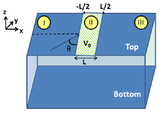
Figure 1: Schematic picture of the system showing the top and bottom surfaces of a TI, a potential barrier with strength $V_{0}$ and width $L$ on the top surface (region $II$), and a wave coming in from region $I$ with an angle of incidence $\theta$.

We will study the effects of two kinds of barriers on the top surface. In Sec. V, we will study what happens if the top surface has a potential barrier which is independent of the $y$ coordinate and has the form $V(x)=V_{0}$ in a region of width $L$. (A schematic picture of this is shown in Fig. 1). The Hamiltonian of this system is given by

$$H_{0}=\begin{pmatrix}H_{top}+V_{0}I_{2}&\lambda I_{2}\\ \lambda I_{2}&H_{bottom}\end{pmatrix}$$ (9)

for $-L/2<x<L/2$, and by Eq. (8) for $x<-L/2$ and $x>L/2$. In Sec. VI, we will study what happens if the top surface has a magnetic barrier of strength $V_{0}$ in a region of width $L$. As explained below, we will choose the direction of the magnetization in the barrier in such a way that the Hamiltonian in the region $-L/2<x<L/2$ has the form

$$H_{0}=\begin{pmatrix}H_{top}+V_{0}\sigma^{x}&\lambda I_{2}\\ \lambda I_{2}&H_{bottom}\end{pmatrix}.$$ (10)

(In Fig. 1, this corresponds to having a barrier with strength $V_{0}\sigma^{x}$ in region $II$). In both cases, our aim will be to study the transmitted charge and spin currents and their dependences on the various parameters of the system, namely, the energy $E$, the coupling between the two surfaces $\lambda$, and the width and height of the potential barrier $L$ and $V_{0}$.

In this paper, we are assuming that the TI is in the form of a thin film whose top and bottom surfaces cover a large area in the $x-y$ plane and whose thickness in the $z$-direction is small. In this situation, which is common for experimental measurements of transport, the contributions of the side surfaces are much smaller than those of the top and bottom surfaces and can therefore be ignored.

III Barrier-free regions

In the barrier-free regions denoted as $I$ and $III$, the Hamiltonian is

$$H_{0}=\begin{pmatrix}0&vke^{i\theta}&\lambda&0\\ vke^{-i\theta}&0&0&\lambda\\ \lambda&0&0&-vke^{i\theta}\\ 0&\lambda&-vke^{-i\theta}&0\end{pmatrix},$$ (11)

where $ke^{i\theta}=k_{y}+ik_{x}$. Thus $k=\sqrt{k_{x}^{2}+k_{y}^{2}}$ and $\theta=\tan^{-1}(k_{x}/k_{y})$. Defining $E=\sqrt{v^{2}k^{2}+\lambda^{2}}$, the eigenvalues of the Hamiltonian in Eq. (11) are

$$e_{1} = e_{2}~{}=~{}-~{}e_{3}~{}=~{}-~{}e_{4}~{}=~{}E,$$ (12)

with corresponding eigenstates

$$|e_{1}\rangle = \frac{1}{2E}~{}\begin{pmatrix}\sqrt{v^{2}k^{2}+\lambda^{2}}\\ \lambda+vke^{-i\theta}\\ \lambda-vke^{i\theta}\\ -\sqrt{v^{2}k^{2}+\lambda^{2}}\end{pmatrix},$$

$$|e_{2}\rangle = \frac{1}{2E}~{}\begin{pmatrix}\sqrt{v^{2}k^{2}+\lambda^{2}}\\ -\lambda+vke^{-i\theta}\\ \lambda+vke^{i\theta}\\ \sqrt{v^{2}k^{2}+\lambda^{2}}\end{pmatrix},$$

$$|e_{3}\rangle = \frac{1}{2E}~{}\begin{pmatrix}-\sqrt{v^{2}k^{2}+\lambda^{2}}\\ \lambda-vke^{-i\theta}\\ \lambda-vke^{i\theta}\\ \sqrt{v^{2}k^{2}+\lambda^{2}}\end{pmatrix},$$

$$|e_{4}\rangle = \frac{1}{2E}~{}\begin{pmatrix}\sqrt{v^{2}k^{2}+\lambda^{2}}\\ \lambda+vke^{-i\theta}\\ -\lambda-vke^{i\theta}\\ \sqrt{v^{2}k^{2}+\lambda^{2}}\end{pmatrix}.$$ (13)

III.1 Wave functions and boundary conditions

In the presence of a potential or a magnetic barrier on the top surface, the reflection and transmission amplitudes can be calculated as follows.

On the top surface, we have three regions: the incident region, the potential region of width $L$, and the transmitted region. Since the Hamiltonian has the Dirac form (i.e., first order in the spatial derivatives), we must match the wave functions (but not their derivatives) at the boundaries between the incident region $I$ and the barrier region (labeled as $II$), and between the barrier region $II$ and the transmitted region $III$. Let these boundaries be at $x=-L/2$ and $x=L/2$. We then have the following wave functions in the three regions.

In the incident region $I$, we consider an incident wave with positive energy, $E=\sqrt{v^{2}k^{2}+\lambda^{2}}$, and one of the eigenstates, say, $|e_{3}\rangle$. There will then be two possible reflected wave functions with the same energy $E$ and amplitudes $r_{1}$ and $r_{2}$. The incident and reflected waves are given by

$$|\psi_{in}\rangle = |e_{3}\rangle e^{i(k_{x}x+k_{y}y)},$$

$$|\psi_{ref}\rangle = (r_{1}|e_{-3}\rangle~{}+~{}r_{2}|e_{-4}\rangle)~{}e^{i(-k_{x}x+k_{y}y)},$$ (14)

where $|e_{3}\rangle$ and $|e_{4}\rangle$ have been defined earlier, and $|e_{-3}\rangle$ and $|e_{-4}\rangle$ can be obtained from those by changing $k_{x}\to-k_{x}$ since these are reflected wave functions. The total wave function in this region is $|\psi_{I}\rangle=|\psi_{in}\rangle+|\psi_{ref}\rangle$.

In the transmitted region $III$, we have two possible wave functions, with amplitudes $t_{1}$ and $t_{2}$. Thus

$$|\psi_{III}\rangle~{}=~{}(t_{1}|e_{3}\rangle~{}+~{}t_{2}|e_{4}\rangle)~{}e^{i(k_{x}x+k_{y}y)}.$$ (15)

We now turn to the barrier region $II$. Since the barrier is independent of the $y$ coordinate, the momentum in the $\hat{y}$ direction, $k_{y}$, and, of course, the energy $E$ will be the same in all the regions. However, the momentum in the $\hat{x}$ direction will generally be different in region $II$ as compared to regions $I$ and $III$. In region $II$, therefore, we will have four different eigenstates having amplitudes $C_{1},C_{2},C_{3}$ and $C_{4}$. Namely, we have

$$|\psi_{II}\rangle = C_{1}|e_{1}^{\prime}\rangle e^{i(k_{x1}^{\prime}x+k_{y}y)}~{}+~{}C_{2}|e_{2}^{\prime}\rangle e^{i(k_{x2}^{\prime}x+k_{y}y)}$$

$$+~{}C_{3}|e_{3}^{\prime}\rangle e^{i(k_{x3}^{\prime}x+k_{y}y)}~{}+~{}C_{4}|e_{4}^{\prime}\rangle e^{i(k_{x4}^{\prime}x+k_{y}y)},$$

where $k_{xi}^{\prime}$ denotes the four possible values of the momentum in region $II$; these four values and the corresponding wave functions $|e_{i}^{\prime}\rangle$ depend on the nature of the barrier (potential and magnetic), and we will present them in Secs. V and VI.

Applying the matching conditions at the boundaries, we obtain

$$|\psi_{I}\rangle = |\psi_{II}\rangle~{}~{}~{}~{}\text{at}~{}~{}~{}x=-L/2,$$

$$|\psi_{II}\rangle = |\psi_{III}\rangle~{}~{}~{}\text{at}~{}~{}~{}x=L/2.$$ (17)

There are thus eight unknowns, $r_{1},r_{2},t_{1},t_{2},C_{1},C_{2},C_{3},C_{4}$, and we have eight equations from matching the four-component wave functions at $x=\pm L/2$. We can therefore solve for the unknowns by writing the eight-dimensional columns $A=(r_{1},r_{2},t_{1},t_{2},C_{1},C_{2},C_{3},C_{4})^{T}$ and $B=(\psi_{in},0,0,0,0)^{T}$ which are related by a matrix $M$ such that $MA=B$; the elements of $M$ are obtained by writing the amplitudes from the various equations above. We can then find the unknowns numerically.

III.2 Basis of eigenstates of $\tau^{x}\sigma^{z}$

Once we obtain the transmission amplitudes $t_{1}$ and $t_{2}$ after solving for the column $A$, the transmitted current and its properties can be studied. This calculation becomes simpler if we make a change of basis as follows. We observe that the Hamiltonian in the barrier-free regions $I$ and $III$ can be written as

$$H_{0}~{}=~{}v\tau^{z}(\sigma^{x}k_{y}-\sigma^{y}k_{x})~{}+~{}\lambda\tau^{x}.$$ (18)

We note that $\tau^{x}\sigma^{z}$ commutes with $H_{0}$. Next, we see that

$$\tau^{x}\sigma^{z}~{}=~{}\begin{pmatrix}0&0&1&0\\ 0&0&0&-1\\ 1&0&0&0\\ 0&-1&0&0\end{pmatrix}$$ (19)

has eigenvalues $\pm 1$ (both doubly degenerate) and corresponding eigenstates of the form

$$|1\rangle~{}=~{}\begin{pmatrix}a\\ b\\ a\\ -b\end{pmatrix}~{}~{}~{}{\rm and}~{}~{}~{}|-1\rangle~{}=~{}\begin{pmatrix}a^{\prime}\\ b^{\prime}\\ -a^{\prime}\\ b^{\prime}\end{pmatrix}.$$ (20)

Since we can find simultaneous eigenstates of $\tau^{x}\sigma^{z}$ and $H_{0}$ in regions $I$ and $III$, we look for eigenstates of $H_{0}$ which have the forms given in Eq. (20) and which satisfy

$$H_{0}|1\rangle = E|1\rangle,$$

$$H_{0}|-1\rangle = E|-1\rangle,$$ (21)

with energy $E=\sqrt{v^{2}k^{2}+\lambda^{2}}$. We find that the eigenstates for the incident waves have the form

$$|1_{in}\rangle = \dfrac{1}{2\sqrt{E}}\begin{pmatrix}\sqrt{E+\lambda}\\ \sqrt{E-\lambda}e^{-i\theta}\\ \sqrt{E+\lambda}\\ -\sqrt{E-\lambda}e^{-i\theta}\end{pmatrix},$$

$$|-1_{in}\rangle = \dfrac{1}{2~{}\sqrt{E}}\begin{pmatrix}\sqrt{E-\lambda}\\ \sqrt{E+\lambda}e^{-i\theta}\\ -\sqrt{E-\lambda}\\ \sqrt{E+\lambda}e^{-i\theta}\end{pmatrix}.$$ (22)

We can see that in the $\lambda\to 0$ limit, there are two linear combinations of the above wave functions which have components only at the top and bottom surfaces, respectively.

To obtain the reflected waves, we change $k_{x}\to-k_{x}$, i.e., $\theta\to-\theta$. This gives

$$|1_{ref}\rangle = \dfrac{1}{2\sqrt{E}}\begin{pmatrix}\sqrt{E+\lambda}\\ \sqrt{E-\lambda}e^{i\theta}\\ \sqrt{E+\lambda}\\ -\sqrt{E-\lambda}e^{i\theta}\end{pmatrix},$$

$$|-1_{ref}\rangle = \dfrac{1}{2\sqrt{E}}\begin{pmatrix}\sqrt{E-\lambda}\\ \sqrt{E+\lambda}e^{i\theta}\\ -\sqrt{E-\lambda}\\ \sqrt{E+\lambda}e^{i\theta}\end{pmatrix}.$$ (23)

Choosing $|1_{in}\rangle$ to be the incident wave, we have

$$|\psi_{I}\rangle = |1_{in}\rangle e^{i(k_{x}x+k_{y})}$$ (24)

$$+~{}(r_{1}|1_{ref}\rangle~{}+~{}r_{2}|-1_{ref}\rangle)~{}e^{i(-k_{x}x+k_{y}y)}$$

in region $I$, and

$$|\psi_{III}\rangle~{}=~{}(t_{1}|1_{in}\rangle~{}+~{}t_{2}|-1_{in}\rangle)~{}e^{i(k_{x}x+k_{y}y)}$$ (25)

in region $III$.

The advantage of working in the basis of eigenstates of $\tau^{x}\sigma^{z}$ is that the charge current, when calculated in regions $I$ and $III$, will not have any cross-terms involving $r_{1},~{}r_{2}$ and $t_{1},~{}t_{2}$. To see this, we note that for the Hamiltonian $H_{0}$, the current operators can be found using the equation of continuity and are given by

$$J_{x} = -v\tau^{z}\sigma^{y}~{}=~{}\begin{pmatrix}0&iv&0&0\\ -iv&0&0&0\\ 0&0&0&-iv\\ 0&0&iv&0\end{pmatrix},$$

$$J_{y} = v\tau^{z}\sigma^{x}~{}=~{}\begin{pmatrix}0&v&0&0\\ v&0&0&0\\ 0&0&0&-v\\ 0&0&-v&0\end{pmatrix}.$$ (26)

We see that both $J_{x}$ and $J_{y}$ commute with the operator $\tau^{x}\sigma^{z}$. We will only study $J_{x}$ below. We now note that

$$\langle 1|J_{x}|-1\rangle = \langle 1|J_{x}(\tau^{x}\sigma^{z})^{2}|-1\rangle$$ (27)

$$= \langle 1|\tau^{x}\sigma^{z}J_{x}\tau^{x}\sigma^{z}|-1\rangle$$

$$= -~{}\langle 1|J_{x}|-1\rangle.$$

This implies that $\langle 1|J_{x}|-1\rangle=0$; hence there will be no cross-terms when we calculate the expectation value of $J_{x}$ in regions $I$ and $III$.

III.3 Conservation of charge current in the $\hat{x}$ direction

Given the wave functions and the form of $J_{x}$, we can calculate $\langle J_{x}\rangle$ in regions $I$ and $III$ and check for conservation of the charge current. In region $I$, we have

$$J_{x}|\psi_{I}\rangle = J_{x}[|1_{in}\rangle e^{i(k_{x}x+k_{y})}$$ (28)

$$+(r_{1}|1_{ref}\rangle+r_{2}|-1_{ref}\rangle)e^{i(-k_{x}x+k_{y}y)}].$$

Since

$$\langle\psi_{I}| = \langle 1_{in}|e^{-i(k_{x}x+k_{y})}$$ (29)

$$+(r_{1}^{*}\langle 1_{ref}|+r_{2}^{*}\langle-1_{ref}|)e^{-i(-k_{x}x+k_{y}y)},$$

we find that

$$\langle\psi_{I}|J_{x}|\psi_{I}\rangle~{}=~{}\dfrac{v\sqrt{E^{2}-\lambda^{2}}}{E}~{}\sin\theta~{}(1-|r_{1}|^{2}-|r_{2}|^{2}).$$ (30)

Using the relation $E^{2}=v^{2}k^{2}+\lambda^{2}$, we can simplify this to obtain

$$\langle J_{x}\rangle_{I}~{}=~{}\dfrac{v^{2}k}{E}~{}\sin\theta~{}(1-|r_{1}|^{2}-|r_{2}|^{2}).$$ (31)

In region $III$, we calculate $\langle\psi_{III}|J_{x}|\psi_{III}\rangle$, and find that

$$\langle J_{x}\rangle_{III}~{}=~{}\dfrac{v^{2}k}{E}~{}\sin\theta~{}(|t_{1}|^{2}+|t_{2}|^{2}).$$ (32)

Equating the expressions in Eqs. (31) and (32), we find that

$$1~{}-~{}|r_{1}|^{2}~{}-~{}|r_{2}|^{2}~{}=~{}|t_{1}|^{2}~{}+~{}|t_{2}|^{2}$$ (33)

in the basis of eigenstates of $\tau^{x}\sigma^{z}$. We have checked numerically that the computed values of the various probabilities satisfy Eq. (33).

We will also calculate the spin current of $\vec{\sigma}$ in the $\hat{x}$ direction by taking the expectation of the operator $J_{x}\sigma^{i}$. Choosing the $\tau^{x}\sigma^{z}$ basis as before, we find that

$$\langle J_{x}\sigma^{y}\rangle_{III}~{}=~{}-\dfrac{v^{2}k}{E}~{}[(t_{1}^{*}t_{2}+t_{1}t_{2}^{*})].$$ (34)

We note that

$$J_{x}\sigma^{y}=-v\tau^{z}.$$ (35)

We therefore anticipate that the expectation values of $J_{x}\sigma^{y}$ will have opposite signs on the two surfaces (which correspond to $\tau^{z}=\pm 1$); this is a consequence of opposite helicities of the Dirac electrons on these surfaces. We will see that this is borne out by the numerical results presented below.

III.4 Differential conductance

Having chosen the incident waves in the basis of eigenstates of $\tau^{x}\sigma^{z}$, we can calculate the transmission probabilities $|t_{i}|^{2}$ and transmitted currents $\langle J_{x}\rangle$. We can then calculate the differential conductance $G$ as follows deb2 . If the system has a large width in the $\hat{y}$ direction given by $W$, the net current going from the left of the barrier to the right is given by

$$I~{}=~{}qW\int\int\frac{dk_{x}dk_{y}}{(2\pi)^{2}}~{}\langle J_{x}\rangle,$$ (36)

where $q$ is the charge of the electrons. We now change variables from $k_{x},~{}k_{y}$ to the energy $E=\hbar v\sqrt{k_{x}^{2}+k_{y}^{2}}$ and the angle of incidence $\theta=\tan^{-1}(k_{x}/k_{y})$ which goes from 0 to $\pi$. If $\mu_{L}$ and $\mu_{R}$ denote the chemical potentials of the left and right leads which are attached to the system, then $E$ goes from $\mu_{R}$ to $\mu_{L}$ in the integral in Eq. (36); we are assuming here that $\mu_{L}>\mu_{R}$. The voltage applied in a lead is related to its chemical potential as $\mu=qV$. In the zero-bias limit, $\mu_{L},~{}\mu_{R}~{}\to~{}\mu$, the differential conductance is given by

$$G~{}=~{}\frac{dI}{dV}~{}=~{}\frac{q^{2}W\mu}{(2\pi v\hbar)^{2}}~{}\int_{0}^{\pi}d\theta~{}\langle J_{x}\rangle.$$ (37)

It is convenient to define a quantity $G_{0}$ which is the maximum possible value of $G$ that arises when the transmission probabilities have the maximum possible values, $|t_{1}|^{2}=|t_{2}|^{2}=1$. Equation (32) then gives $\langle J_{x}\rangle=2v\sqrt{1-\lambda^{2}/\mu^{2}}\sin\theta$, where we have used the relations $E=\mu$ and $vk=\sqrt{E^{2}-\lambda^{2}}$. The conductance in this case is given by

$$G_{0}~{}=~{}\frac{q^{2}W}{v(\pi\hbar)^{2}}~{}\sqrt{\mu^{2}~{}-~{}\lambda^{2}}.$$ (38)

In the figures presented below, we will plot the dimensionless ratio $G/G_{0}$ whose maximum possible value is 1. In the plots, the conductance will be calculated at a value of the incident electron energy $E$ which is equal to $\mu$. We will always choose $E$ to lie in the range $\lambda<E<m$, so that the energy lies in the upper (positive energy) band of the surface states but in the gap of the bulk states; hence the bulk states will not contribute to the conductance.

IV $\delta$-function barrier

Before studying the more realistic case of barriers with finite widths, it turns out to be instructive to study the simpler problem of a $\delta$-function barrier. This can be thought of as the limit of a finite width barrier in which the barrier height $V_{0}\to\infty$ and barrier width $L\to 0$, keeping the product $V_{0}L=c$ fixed. We will discover later that many of the results obtained for barriers with finite widths can be understood qualitatively by considering the problem of $\delta$-function barriers.

IV.1 $\delta$-function potential barrier  -  single surface

We first consider the case of a single surface of a TI with a potential barrier of the form $V_{0}\delta(x)$. For a single surface, the wave function is a two-component object. Due to the Dirac nature of the Hamiltonian, we find that a $\delta$-function barrier produces a discontinuity in the wave function. To show this, we consider

$$H = v(-i\sigma^{x}\partial_{y}+i\sigma^{y}\partial_{x})~{}+~{}c~{}\delta(x),$$

$$H\psi = E\psi.$$ (39)

Following a procedure similar to the one used to study the effect of a $\delta$-function barrier in a Schrödinger equation, we integrate the second equation in Eq. (39) through the $\delta$-function at $x=0$. This gives a matching condition at $x=0$ of the form

$$\psi_{x\to 0^{+}}=e^{i(c/v)\sigma^{y}}\psi_{x\to 0^{-}}.$$ (40)

For $x<0$, the wave function has an incident part with amplitude 1 and a reflected part with amplitude $r$; for $x>0$, the wave function has a transmitted part with amplitude $t$. We therefore have

$$\psi_{x\to 0^{-}} = \begin{pmatrix}1\\ e^{-i\theta}\end{pmatrix}~{}+~{}r\begin{pmatrix}1\\ e^{i\theta}\end{pmatrix},$$

$$\psi_{x\to 0^{+}} = t\begin{pmatrix}1\\ e^{-i\theta}\end{pmatrix}.$$ (41)

Equation (40) then gives

$$t\begin{pmatrix}1\\ e^{-i\theta}\end{pmatrix} = \begin{pmatrix}\cos(c/v)&\sin(c/v)\\ -\sin(c/v)&\cos(c/v)\end{pmatrix}$$ (42)

$$\times~{}\bigg{[}\begin{pmatrix}1\\ e^{-i\theta}\end{pmatrix}~{}+~{}r\begin{pmatrix}1\\ e^{i\theta}\end{pmatrix}\bigg{]}.$$

The above equation gives two equations involving two variables $r$ and $t$. Solving them we obtain

$$r = \dfrac{\sin(c/v)~{}(1~{}+~{}e^{-i2\theta})}{2~{}[i\cos(c/v)\sin\theta~{}-~{}\sin(c/v)]},$$

$$t = \dfrac{i\sin\theta}{i\cos(c/v)\sin\theta~{}-~{}\sin(c/v)}.$$ (43)

It can be verified that $|r|^{2}+|t|^{2}$ =1. For $c/v=2n\pi$, we find that $t=1$ and $r=0$, while for $c/v=(2n+1)\pi$, we get $t=-1$ and $r=0$.

IV.2 $\delta$-function potential barrier  -  two surfaces

Next we consider the case where we have top and bottom surfaces of a TI with a coupling $\lambda$ between them. We apply a $\delta$-function potential barrier $V_{0}\delta(x)$ to only the top surface. The wave function $\psi$ now has four components with the first two corresponding to the top surface and the last two to the bottom. The boundary condition at $x=0$ on the top surface remains the same as in the previous section. Using the wave vectors obtained in Eq. (22) and Eq. (23) in order to obtain the condition from Eq. (40), we get

$$t_{1}|1_{in}\rangle~{}+~{}t_{2}|-1_{in}\rangle$$

$$=~{}\Lambda_{0}~{}\left[|1_{in}\rangle~{}+~{}r_{1}|1_{ref}\rangle~{}+~{}r_{2}|-1_{ref}\rangle\right],$$ (44)

where the matrix $\Lambda_{0}$ is given by

$$\Lambda_{0} = \begin{pmatrix}\cos(c/v)&\sin(c/v)&0&0\\ -\sin(c/v)&\cos(c/v)&0&0\\ 0&0&1&0\\ 0&0&0&1\end{pmatrix},$$ (45)

$r_{1}$ and $t_{1}$ are the reflection and transmission amplitudes for $|1_{in}\rangle$, $r_{2}$ and $t_{2}$ are the reflection and transmission amplitudes for $|-1_{in}\rangle$, and the incident wave vector has been chosen to be $|1_{in}\rangle$.

Solving the four-component equation in Eq. (44), we get, for $c/v=2n\pi$,

$$r_{1}=0,~{}~{}~{}r_{2}=0,~{}~{}~{}t_{1}=1,~{}~{}~{}\text{and}~{}~{}~{}t_{2}=0.$$ (46)

If we choose the incident wave vector to be $|-1_{in}\rangle$, we get

$$r_{1}=0,~{}~{}~{}r_{2}=0,~{}~{}~{}t_{1}=0,~{}~{}~{}\text{and}~{}~{}~{}t_{2}=1.$$ (47)

For $c/v=(2n+1)\pi$, we obtain from Eq. (44)

$$r_{2} = 0,~{}~{}~{}~{}t_{1}~{}=~{}0,$$

$$r_{1} = \dfrac{\lambda e^{-i\theta}}{iE\sin\theta-\lambda\cos\theta},$$

$$t_{2} = -~{}\dfrac{i\sin\theta\sqrt{E^{2}-\lambda^{2}}}{iE\sin\theta-\lambda\cos\theta}.$$ (48)

In contrast to the case of a single surface with $c/v$ equal to an odd multiple of $\pi$, we see that that the reflection amplitude does not vanish completely. In Eq. (48), we see that as $\lambda\to 0$, $r_{1}\to 0$ and $t_{2}\to-1$. As $\lambda\to E$, $t_{2}\to 0$ and $r_{1}\to-1$. Similarly for $|-1_{in}\rangle$ as the incident wave vector, we obtain

$$r_{1} = 0,~{}~{}~{}~{}t_{2}~{}=~{}0,$$

$$r_{2} = -~{}\dfrac{\lambda e^{-i\theta}}{iE\sin\theta~{}+~{}\lambda\cos\theta},$$

$$t_{1} = -~{}\dfrac{i\sin\theta\sqrt{E^{2}-\lambda^{2}}}{iE\sin\theta~{}+~{}\lambda\cos\theta}.$$ (49)

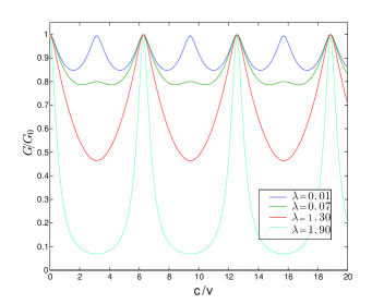
Figure 2: Conductance as a function of $c/v$ for different couplings $\lambda$, when both incident waves are present, and $E=2$.

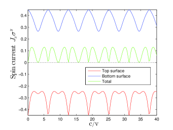
Figure 3: Transmitted spin currents (in units of $v$) as a function of $c/v$ when both incident waves are present, $E=2$ and $\lambda=1$.

In Figs. 2 and 3, we show the differential conductance and spin currents as a function of $c/v$ for certain values of $\lambda$; in both cases, we assume that both incident waves $|1_{in}\rangle$ and $|-1_{in}\rangle$ are present, and we integrate over the angle of incidence $\theta$. Figure 2 shows that the oscillation period of the conductance as a function of $c/v$ changes from $\pi$ to $2\pi$ as $\lambda$ increases; the amplitude of the oscillations increases as $\lambda$ increases from 0 to $E$. These observations agree with our analytic results for a single surface and two coupled surfaces. In Fig. 3 we show the transmitted spin currents integrated over $\theta$ at the top and bottom surfaces as a function of $c/v$. As mentioned above, the spin current at the top (bottom) surface is negative (positive) although the sum of the two is positive. The oscillation period at both surfaces is $2\pi$. (In Figs. 2-5, the values of $E$ and $\lambda$ are in units of $0.01$ eV, $c/v$ is in units of $\hbar$, and $\langle J_{x}\sigma^{y}\rangle$ is in units of $v$).

IV.3 $\delta$-function magnetic barrier  -  single surface

Now we consider a $\delta$-function magnetic barrier of the form $V_{0}\delta(x)\sigma^{x}$ on the surface of a TI. We have

$$H = v(-i\sigma^{x}\partial_{y}+i\sigma^{y}\partial_{x})~{}+~{}c~{}\delta(x)~{}\sigma^{x},$$

$$H\psi = E\psi.$$ (50)

Integrating over the $\delta$-function at $x=0$ now gives the following matching condition for the wave function,

$$\psi_{x\to 0^{+}}~{}=~{}e^{(c/v)\sigma^{z}}\psi_{x\to 0^{-}}.$$ (51)

(Interestingly, Eqs. (40) and (51) both satisfy continuity of the current $\psi^{\dagger}J_{x}\psi$ at $x=0$, although Eq. (40) is a unitary transformation while Eq. (51) is not). Using the same wave functions as in the case of a $\delta$-function potential barrier, we obtain

$$t\begin{pmatrix}1\\ e^{-i\theta}\end{pmatrix}~{}~{}=~{}~{}\begin{pmatrix}e^{c/v}&0\\ 0&e^{-c/v}\end{pmatrix}\bigg{[}\begin{pmatrix}1\\ e^{-i\theta}\end{pmatrix}~{}+~{}r\begin{pmatrix}1\\ e^{i\theta}\end{pmatrix}\bigg{]}.$$ (52)

Solving for $r$ and $t$, from the two conditions above, we get

$$r = -~{}\dfrac{e^{-2c/v}-1}{e^{-2c/v}e^{i2\theta}-1},$$

$$t = \dfrac{e^{-c/v}(e^{i2\theta}-1)}{e^{-2c/v}e^{i2\theta}-1}.$$ (53)

It can be checked that $|r|^{2}+|t|^{2}=1$. In the limit $c/v\to\infty$, we get $r=-1$ and $t=0$. Hence the transmission probability goes to zero as the strength of the barrier increases; this is in contract to the $\delta$-function potential barrier where the transmission probability oscillates with the barrier strength.

IV.4 $\delta$-function magnetic barrier  -  two surfaces

Similar to the case of a $\delta$-function potential barrier, we apply a $\delta$-function magnetic barrier on the top surface of a TI, with the bottom surface being coupled to the top with the coupling $\lambda$ as usual. The same boundary condition in this case gives the following equation for the case that the incident wave vector is chosen to be $|1_{in}\rangle$,

$$t_{1}|1_{in}\rangle~{}+~{}t_{2}|-1_{in}\rangle$$

$$=~{}\Lambda_{1}~{}\left[|1_{in}\rangle~{}+~{}r_{1}|1_{ref}\rangle~{}+~{}r_{2}|-1_{ref}\rangle\right],$$ (54)

where the matrix $\Lambda_{1}$ is given by

$$\Lambda_{1} = \begin{pmatrix}\exp(c/v)&0&0&0\\ 0&\exp(-c/v)&0&0\\ 0&0&1&0\\ 0&0&0&1\end{pmatrix}.$$ (55)

Here $r_{1}$ and $t_{1}$ are the reflection and transmission amplitude of $|1_{in}\rangle$, and $r_{2}$ and $t_{2}$ are the reflection and transmission amplitude of $|-1_{in}\rangle$. Upon solving these equations in the limit $c/v\to\infty$, we get

$$t_{1} = \dfrac{\sin\theta~{}(E^{2}-\lambda^{2})}{(2E^{2}-\lambda^{2})\sin\theta~{}-~{}i\lambda^{2}\cos\theta},$$

$$r_{1} = -~{}\dfrac{E\sin\theta~{}(E+\lambda)~{}+~{}\lambda^{2}e^{-i\theta}}{(2E^{2}-\lambda^{2})\sin\theta~{}-~{}i\lambda^{2}\cos\theta},$$

$$r_{2} = -~{}\dfrac{E\sin\theta~{}\sqrt{E^{2}-\lambda^{2}}}{(2E^{2}-\lambda^{2})\sin\theta~{}-~{}i\lambda^{2}\cos\theta},$$

$$t_{2} = -~{}\dfrac{\sin\theta(E-\lambda)~{}\sqrt{E^{2}-\lambda^{2}}}{(2E^{2}-\lambda^{2})\sin\theta~{}-~{}i\lambda^{2}\cos\theta}.$$ (56)

We see that unless $E\to\lambda$, the transmission probability does not vanish even in the limit of $c/v\to\infty$. This is because the bottom surface (which does not have a magnetic barrier) allows for the conduction of electrons since it is coupled to the top surface.

Figure 4 shows the differential conductance as a function of $c/v$ for various values of $\lambda$; we see that there are no oscillations, unlike the case of a $\delta$-function potential barrier (Fig. 2). For a very large value of $c/v$, the conductance does not vanish but reaches a constant value. However, as $\lambda$ approaches $E$, the conductance approaches zero for a large barrier. This matches with the analytic expressions presented in Eqs. (56). Figure 5 shows the transmitted spin current as a function of $c/v$; this too does not show any oscillations.

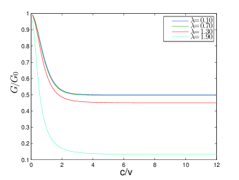
Figure 4: Conductance as a function of $c/v$ for different values of $\lambda$, when both incident waves are present, and $E=2$.

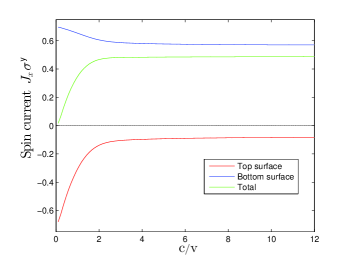
Figure 5: Transmitted spin currents (in units of $v$) integrated over $\theta$ as a function of $c/v$, when both incident waves are present, $E=2$ and $\lambda=1$.

V Potential barrier with finite width

We now study the case of a finite width potential barrier on the top surface. In region $II$ where the potential is nonzero, the Hamiltonian is

$$H_{II}=\begin{pmatrix}V_{0}&vk^{\prime}e^{i\theta^{\prime}}&\lambda&0\\ vk^{\prime}e^{-i\theta^{\prime}}&V_{0}&0&\lambda\\ \lambda&0&0&-vk^{\prime}e^{i\theta^{\prime}}\\ 0&\lambda&-vk^{\prime}e^{-i\theta^{\prime}}&0\end{pmatrix}$$ (57)

The eigenvalues of $H_{II}$ and the respective eigenstates are

$$e_{1}^{\prime} = \dfrac{V_{0}}{2}+\dfrac{1}{2}\sqrt{(V_{0}+2vk^{\prime})^{2}+4\lambda^{2}}$$

$${\rm and}~{}~{}~{}|e_{1}^{\prime}\rangle = \frac{1}{\sqrt{2(1+\alpha_{1}^{2})}}~{}\begin{pmatrix}1\\ e^{-i\theta^{\prime}}\\ \alpha_{1}\\ \alpha_{1}e^{-i\theta^{\prime}}\end{pmatrix},$$

$$e_{2}^{\prime} = \dfrac{V_{0}}{2}-\dfrac{1}{2}\sqrt{(V_{0}+2vk^{\prime})^{2}+4\lambda^{2}}$$

$${\rm and}~{}~{}~{}|e_{2}^{\prime}\rangle = \frac{1}{\sqrt{2(1+\alpha_{2}^{2})}}~{}\begin{pmatrix}1\\ e^{-i\theta^{\prime}}\\ \alpha_{2}\\ \alpha_{2}e^{-i\theta^{\prime}}\end{pmatrix},$$

$$e_{3}^{\prime} = \dfrac{V_{0}}{2}+\dfrac{1}{2}\sqrt{(V_{0}-2vk^{\prime})^{2}+4\lambda^{2}}$$

$${\rm and}~{}~{}~{}|e_{3}^{\prime}\rangle = \frac{1}{\sqrt{2(1+\alpha_{3}^{2})}}~{}\begin{pmatrix}1\\ -e^{-i\theta^{\prime}}\\ \alpha_{3}\\ -\alpha_{3}e^{-i\theta^{\prime}}\end{pmatrix},$$

$$e_{4}^{\prime} = \dfrac{V_{0}}{2}-\dfrac{1}{2}\sqrt{(V_{0}-2vk^{\prime})^{2}+4\lambda^{2}}$$

$${\rm and}~{}~{}~{}|e_{4}^{\prime}\rangle = \frac{1}{\sqrt{2(1+\alpha_{4}^{2})}}~{}\begin{pmatrix}1\\ -e^{-i\theta^{\prime}}\\ \alpha_{4}\\ -\alpha_{4}e^{-i\theta^{\prime}}\end{pmatrix},$$ (58)

where

$$\alpha_{1} = \dfrac{-V_{0}-2vk^{\prime}+\sqrt{(V_{0}+2vk^{\prime})^{2}+4\lambda^{2}}}{2\lambda},$$

$$\alpha_{2} = \dfrac{-V_{0}-2vk^{\prime}-\sqrt{(V_{0}+2vk^{\prime})^{2}+4\lambda^{2}}}{2\lambda},$$

$$\alpha_{3} = \dfrac{-V_{0}+2vk^{\prime}+\sqrt{(V_{0}-2vk^{\prime})^{2}+4\lambda^{2}}}{2\lambda},$$

$$\alpha_{4} = \dfrac{-V_{0}+2vk^{\prime}-\sqrt{(V_{0}-2vk^{\prime})^{2}+4\lambda^{2}}}{2\lambda},$$

$$k^{\prime}e^{i\theta^{\prime}} = k_{y}+ik_{x}^{\prime}~{}~{}~{}{\rm and}~{}~{}~{}k^{{}^{\prime}2}~{}=~{}k_{x}^{{}^{\prime}2}+k_{y}^{2}.$$ (59)

[In the limit $\lambda\to 0$, we note that the states labeled 1 and 3 reduce to states at the top surface (namely, $e_{1}^{\prime}\to V_{0}+vk^{\prime}$, $e_{3}^{\prime}\to V_{0}-vk^{\prime}$, and the lower two components of $|e_{1}^{\prime}\rangle$ and $|e_{3}^{\prime}\rangle\to 0$), while states 2 and 4 reduce to states at the bottom surface (namely, $e_{2}^{\prime}\to-vk^{\prime}$, $e_{4}^{\prime}\to vk^{\prime}$, and the upper two components of $|e_{2}^{\prime}\rangle$ and $|e_{4}^{\prime}\rangle\to 0$. We have assumed here that $V_{0}\pm 2vk^{\prime}>0$]. To find the allowed values of $k_{x}^{\prime}$, we note that $k_{y}$ is conserved, i.e., has the same value as in the barrier-free region, because the potential is independent of $y$. We now equate the four eigenvalues shown in Eq. (58) to the energy $E$ in the barrier-free region since the energy is conserved. We then obtain for $k^{\prime}$ the expression

$$k^{\prime}~{}=~{}\pm\frac{1}{2v}(V_{0}\pm\sqrt{(2E-V_{0})^{2}-4\lambda^{2}}),$$ (60)

in which all four combinations of plus and minus signs can appear. We then find that

$$k_{x1}^{\prime} = \sqrt{\dfrac{1}{v^{2}}\bigg{(}-\dfrac{V_{0}}{2}+\sqrt{\big{(}E-\dfrac{V_{0}}{2}\big{)}^{2}-\lambda^{2}}\bigg{)}^{2}-k_{y}^{2}}~{},$$

$$k_{x2}^{\prime} = -~{}\sqrt{\dfrac{1}{v^{2}}\bigg{(}-\dfrac{V_{0}}{2}+\sqrt{\big{(}E-\dfrac{V_{0}}{2}\big{)}^{2}-\lambda^{2}}\bigg{)}^{2}-k_{y}^{2}}~{},$$

$$k_{x3}^{\prime} = \sqrt{\dfrac{1}{v^{2}}\bigg{(}-\dfrac{V_{0}}{2}-\sqrt{\big{(}E-\dfrac{V_{0}}{2}\big{)}^{2}-\lambda^{2}}\bigg{)}^{2}-k_{y}^{2}}~{},$$

$$k_{x4}^{\prime} = -~{}\sqrt{\dfrac{1}{v^{2}}\bigg{(}-\dfrac{V_{0}}{2}-\sqrt{\big{(}E-\dfrac{V_{0}}{2}\big{)}^{2}-\lambda^{2}}\bigg{)}^{2}-k_{y}^{2}}~{}.$$

V.1 Numerical results

We will now present our results for the transmission probabilities $|t_{1}|^{2}$ and $|t_{2}|^{2}$, transmitted current $\langle J_{x}\rangle$, the differential conductance $G/G_{0}$, and the transmitted spin current $\langle J_{x}\sigma^{y}\rangle$ for various parameter values. In all the plots, the values of $E$, $\lambda$ and $V_{0}$ are in units of $0.01$ eV, the barrier width $L$ is in units of $\hbar v/(0.02$ eV) $~{}\simeq 17$ nm, and the currents are in units of $v$ (we have taken $v=0.333$ eV-nm as in Bi₂Se₃). We have chosen these units of energy and barrier width as they are experimentally realistic (see Ref. kats, where tunneling through barriers in single- and bilayer graphene was studied). Further, we want the incident energy $E$ to be much smaller than $m=0.28$ eV (for Bi₂Se₃) so that the bulk states do not contribute to the conductance.

Figures 6 show the transmitted probabilities $|t_{i}|^{2}$ and currents $\langle J_{x}\rangle$ for different choices of the incident waves. In Fig. 6 (a), where the incident wave has been chosen to be $|1_{in}\rangle$, we see that $|t_{1}|^{2}$ is symmetric about $\theta=\pi/2$, whereas $|t_{2}|^{2}$, which is the probability of $|-1_{in}\rangle$ in region $III$, is asymmetric. Similarly, in Fig. 6 (b), where the incident wave is $|-1_{in}\rangle$, we see that $|t_{2}|^{2}$ is symmetric, whereas $|t_{1}|^{2}$, which is the probability of $|1_{in}\rangle$ in region $III$, is asymmetric about $\theta=\pi/2$. In Fig. 6 (c), both are symmetric as the transmitted current gets an equal contribution from the two waves, $|1_{in}\rangle$ and $|-1_{in}\rangle$; this makes $|t_{1}|^{2}$, $|t_{2}|^{2}$ and the total current symmetric about $\theta=\pi/2$. We can understand these symmetries as follows.

$\sigma^{y}$ symmetry: The symmetry between $|t_{1}|^{2}$ and $|t_{2}|^{2}$ at the incident angles $\theta$ and $\pi-\theta$ can be understood by looking at the effect of a unitary transformation by the operator $\sigma^{y}$. We observe that

(i)  $\sigma^{y}H(k_{x},k_{y})\sigma^{y}=H(k_{x},-k_{y})$, where $H(k_{x},k_{y})$ is the total Hamiltonian in region $II$ given by

$$H(k_{x},k_{y})~{}=~{}v\tau^{z}(\sigma^{x}k_{y}-\sigma^{y}k_{x})~{}+~{}\lambda\tau^{x}~{}+~{}\frac{V_{0}}{2}(1+\tau^{z}).$$ (62)

(ii)  Since $\sigma^{y}$ anticommutes with $\sigma^{z}$, we have $\tau^{x}\sigma^{z}\sigma^{y}=-\sigma^{y}\tau^{x}\sigma^{z}$. Hence $\sigma^{y}$ changes the eigenvalue of $\tau^{x}\sigma^{z}$ from $+1$ to $-1$, thus changing $|1_{in}\rangle$ to $|-1_{in}\rangle$, and vice versa.

Using the above results, we can understand why (i) $|t_{1}|^{2}$ in Fig. 6 (a) and $|t_{2}|^{2}$ in Fig. 6 (b) are related by $k_{y}\to-k_{y}$, i.e., by $\theta\to\pi-\theta$, and (ii) $|t_{2}|^{2}$ in Fig. 6 (a) and $|t_{1}|^{2}$ in Fig. 6 (b) are also related by $\theta\to\pi-\theta$. These symmetries imply that the total transmission probability, $|t_{1}|^{2}+|t_{2}|^{2}$, when both incident waves are present, must be symmetric under $\theta\to\pi-\theta$. This is consistent with Fig. 6 (c).

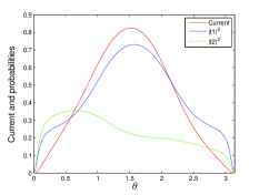
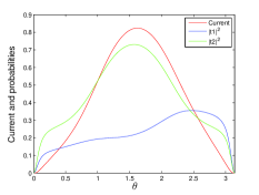
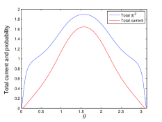
Figure 6: Transmitted currents (in units of $v$) and probabilities as a function of $\theta$ when (a) the incident wave is $|1_{in}\rangle$, (b) the incident wave function is $|-1_{in}\rangle$, and (c) both incident waves are present. We have taken $E=2$, $\lambda=1$, $V_{0}=1$, and $L=1$.

In Fig. 7, the conductance has been plotted as a function of $V_{0}L/v$ (which is in units of $\hbar$). The conductance is seen to oscillate with a period which depends on the parameter $\lambda$. The conductance decreases with increase in $\lambda$ as expected. An interesting phenomenon is that for small values of $\lambda$ (much smaller than the incident energy $E$), the period of oscillation of the current with $V_{0}L/v$ is $\pi$. However, for large values of $\lambda$, comparable to $E$, the oscillation period is $2\pi$, which is twice the previous value. The oscillation period for small $\lambda$ can been understood analytically as follows. For $\lambda\simeq 0$, the top and bottom states are decoupled, and we can find the transmitted amplitudes analytically. For $V_{0}\gg E$, we find that

$$|t_{1}|^{2}~{}=~{}\dfrac{\sin^{2}\theta}{\sin^{2}(V_{0}L/v)\cos^{2}\theta~{}+~{}\sin^{2}\theta}.$$ (63)

It is clear that the maxima of $|t_{1}|^{2}$ lie at $V_{0}L/v=n\pi$. For $\lambda$ close to $E$, we do not have an analytical expression for $|t_{1}|^{2}$, and we therefore do not have an analytical understanding of the oscillation period. However, we have gained some understanding of this by looking at the limit of a $\delta$-function potential barrier in Sec. IV.

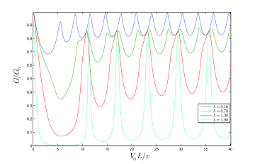
Figure 7: Conductance versus $V_{0}L/v$ for different values of $\lambda$, with $E=2$ and $L=1$.

V.2 Currents at the top and bottom surfaces

It is interesting to look at the currents at the top and bottom surfaces separately. (It may be possible to experimentally detect these currents by attaching leads to the system which couple differently to the top and bottom surfaces). This is done by taking the projections of the previously obtained transmitted wave functions on to the top and bottom surfaces (i.e., taking the upper and lower two components, respectively) and then calculating the expectation value of $J_{x}$ for these wave functions. (In Eq. (26), we note that $J_{x}$ is block diagonal in the basis of top and bottom surface states).

In region $III$, we have

$$|1_{in}\rangle = \dfrac{1}{2\sqrt{E}}\begin{pmatrix}\sqrt{E+\lambda}\\ \sqrt{E-\lambda}e^{-i\theta}\\ \sqrt{E+\lambda}\\ -\sqrt{E-\lambda}e^{-i\theta}\end{pmatrix},$$

$$|-1_{in}\rangle = \dfrac{1}{2\sqrt{E}}\begin{pmatrix}\sqrt{E-\lambda}\\ \sqrt{E+\lambda}e^{-i\theta}\\ -\sqrt{E-\lambda}\\ \sqrt{E+\lambda}e^{-i\theta}\end{pmatrix}.$$ (64)

For the top and bottom surfaces,

$$|\psi_{III,t/b}\rangle~{}=~{}(t_{1}|1_{in,t/b}\rangle~{}+~{}t_{2}|-1_{in,t/b}\rangle)~{}e^{i(k_{x}x+k_{y}y)},$$ (65)

where $|1_{in,t/b}\rangle=[(1\pm\tau^{z})/2]|1_{in}\rangle$ and $|-1_{in,t/b}\rangle=[(1\pm\tau^{z})/2]|-1_{in}\rangle$. Namely,

$$|1_{in,t}\rangle = \dfrac{1}{2\sqrt{E}}\begin{pmatrix}\sqrt{E+\lambda}\\ \sqrt{E-\lambda}e^{-i\theta}\\ 0\\ 0\end{pmatrix},$$

$$|-1_{in,t}\rangle = \dfrac{1}{2\sqrt{E}}\begin{pmatrix}\sqrt{E-\lambda}\\ \sqrt{E+\lambda}e^{-i\theta}\\ 0\\ 0\end{pmatrix},$$ (66)

are the wave functions at the top surface, and

$$|1_{in,b}\rangle = \dfrac{1}{2\sqrt{E}}\begin{pmatrix}0\\ 0\\ \sqrt{E+\lambda}\\ -\sqrt{E-\lambda}e^{-i\theta}\end{pmatrix},$$

$$|-1_{in,b}\rangle = \dfrac{1}{2\sqrt{E}}\begin{pmatrix}0\\ 0\\ -\sqrt{E-\lambda}\\ \sqrt{E+\lambda}e^{-i\theta}\end{pmatrix},$$ (67)

are the wave functions at the bottom surface. Since $J_{x}$ is block diagonal in this basis, we can calculate $\langle J_{x,t/b}\rangle$ where

$$J_{x,t}~{}=~{}\frac{1~{}+~{}\tau^{z}}{2}~{}J_{x}~{}~{}~{}~{}{\rm and}~{}~{}~{}~{}J_{x,b}~{}=~{}\frac{1~{}-~{}\tau^{z}}{2}~{}J_{x}.$$ (68)

We then get for the top and bottom surfaces

$$\langle\psi_{III,t}|J_{x,t}|\psi_{III,t}\rangle~{}=~{}\dfrac{v^{2}k}{2E}\sin\theta~{}(|t_{1}|^{2}+|t_{2}|^{2})$$

$$+ \dfrac{v}{2E}~{}[E\sin\theta(t_{1}^{*}t_{2}+t_{1}t_{2}^{*})~{}+~{}i\lambda\cos\theta(t_{1}^{*}t_{2}-t_{1}t_{2}^{*})],$$

$$\langle\psi_{III,b}|J_{x,b}|\psi_{III,b}\rangle~{}=~{}\dfrac{v^{2}k}{2E}\sin\theta~{}(|t_{1}|^{2}+|t_{2}|^{2})$$

$$- \dfrac{v}{2E}[E\sin\theta(t_{1}^{*}t_{2}+t_{1}t_{2}^{*})~{}+~{}i\lambda\cos\theta(t_{1}^{*}t_{2}-t_{1}t_{2}^{*})].$$

Note that the cross-terms do not vanish when we calculate the currents at the top and bottom surfaces separately, and these terms appear with opposite signs at the two surfaces.

Note that when $V_{0}=0$, i.e., there is no scattering, we have no cross-terms since either $t_{1}$ or $t_{2}$ vanishes depending on whether the incident wave is $|1_{in}\rangle$ or $|-1_{in}\rangle$. We then get equal currents at the top and bottom surfaces,

$$\langle\psi_{III,t}|J_{x,t}|\psi_{III,t}\rangle~{}=~{}\langle\psi_{III,b}|J_{x,b}|\psi_{III,b}\rangle.$$ (70)

The difference between the currents at the two surfaces is therefore a measure of the barrier strength $V_{0}$.

Using the expressions in Eq. (LABEL:tb1), we obtain the results shown in Figs. 8 for the currents at the top and bottom surfaces as a function of $\theta$. Interestingly, these figures show that the currents at the top and bottom surfaces separately can have negative values for certain ranges of $\theta$ when only one one of the incident waves is present. This means that some current flows from the top surface to the bottom surface or vice versa. (Typically this happens close to a glancing angle of incidence, i.e., $\theta\gtrsim 0$ and $\theta\lesssim\pi$). However the total current when both incident waves are present is positive for all values of $\theta$ at both surfaces; we can see this in Fig. 8 (c). We also note that the individual currents are not symmetric about $\theta=\pi/2$ (normal incidence) although the total current is symmetric about $\theta=\pi/2$.

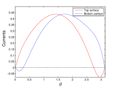
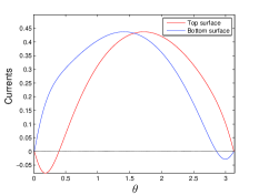
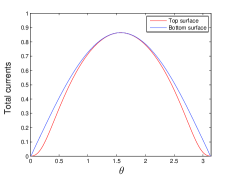
Figure 8: Transmitted currents (in units of $v$) at the top and bottom surfaces as a function of $\theta$ when (a) the incident wave is $|1_{in}\rangle$, (b) the incident wave function is $|-1_{in}\rangle$, and (c) both incident waves are present. We have taken $E=2$, $\lambda=1$, $V_{0}=0.25$, and $L=1$.

Figures 9 (a), 9 (b) and 9 (c) show how the conductances at the top and bottom surfaces vary with $V_{0}L/v$. For small values of the coupling $\lambda$, the bottom surface conducts independently of the top surface and gives a constant current, while the current at the top surface oscillates with a period $\pi$. As we increase $\lambda$, the current at the bottom surface also begins to develop an oscillatory behavior. Finally, when $\lambda$ is close to $E$, there are sharp peaks which occur with a period equal to $2\pi$. The variation of the period as $\lambda$ increases from zero to $E$ is similar to the results that we found for a $\delta$-function potential barrier in Sec. IV.2.

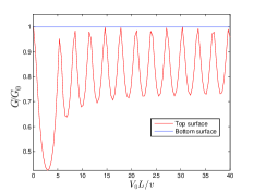
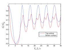
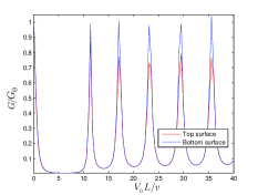
Figure 9: Conductances at the top and bottom surfaces versus $V_{0}L/v$ for (a) a small value of $\lambda=0.01$, (b) an intermediate value of $\lambda=1$, and (c) a value of $\lambda=1.9$ close to $E$. We have taken $E=2$ and $L=1$.

Similarly, we can obtain the expressions for the spin current ($J_{x}\sigma^{y}$) as discussed in Eqs. (34) and (35). For the top and bottom surfaces separately, we have to calculate the expectation values of $-(v/2)(1+\tau^{z})$ and $(v/2)(1-\tau^{z})$, respectively; this gives

$$\langle J_{x}\sigma^{y}\rangle_{t} = -~{}\dfrac{v}{2}~{}\big{[}|t_{1}|^{2}+|t_{2}|^{2}+\dfrac{vk}{E}(t_{1}^{*}t_{2}+t_{1}t_{2}^{*})\big{]},$$

$$\langle J_{x}\sigma^{y}\rangle_{b} = \dfrac{v}{2}~{}\big{[}|t_{1}|^{2}+|t_{2}|^{2}-\dfrac{vk}{E}(t_{1}^{*}t_{2}+t_{1}t_{2}^{*})\big{]}.$$ (71)

In contrast to Eqs. (LABEL:tb1) for the currents at the top and bottom surfaces, we see that the cross-terms for the spin current appear with the same sign at the two surfaces. For $V_{0}=0$, there are no cross-terms and the spin currents at the top and bottom surfaces have opposite values,

$$\langle J_{x}\sigma^{y}\rangle_{t}~{}=~{}-~{}\langle J_{x}\sigma^{y}\rangle_{b}.$$ (72)

The total spin current is then zero. Hence the total spin current is a measure of the barrier strength $V_{0}$.

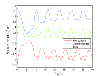
Figure 10: Total spin currents (in units of $v$) as a function of $V_{0}L/v$ when both incident waves are present, for $E=2$, $\lambda=1$, and $L=1$.

In Fig. 10, we show the total spin currents as a function of $V_{0}L/v$ when both incident waves are present. Once again we see oscillations, the period of the largest oscillations being $2\pi$. Note also that the spin current is always negative (positive) at the top (bottom) surface as was mentioned after Eq. (35).

VI Magnetic barrier with finite width

In Sec. V, we have studied the effects of a potential barrier with strength $V_{0}$ on the top surface. We will now study what happens if we replace the potential barrier by a magnetic barrier of the form $V_{0}\sigma^{x}$. This may be experimentally realized by placing a strip of a ferromagnetic material on the top surface whose magnetization points along the $\hat{x}$ direction and has a Zeeman coupling to the spin of the surface electrons. (For convenience, we will include both the magnetization of the ferromagnetic strip and its coupling to the electron spin in the definition of $V_{0}$ so that it has dimensions of energy). The Hamiltonian in the barrier region $II$ is now given by

$$H_{II}=\begin{pmatrix}0&vk^{\prime}e^{i\theta^{\prime}}+V_{0}&\lambda&0\\ vk^{\prime}e^{-i\theta^{\prime}}+V_{0}&0&0&\lambda\\ \lambda&0&0&-vk^{\prime}e^{i\theta^{\prime}}\\ 0&\lambda&-vk^{\prime}e^{-i\theta^{\prime}}&0\end{pmatrix}.$$ (73)

The eigenvalues of this are found to be

$$e_{1}^{\prime} = \sqrt{E^{2}+V_{0}vk^{\prime}\cos\theta^{\prime}+\frac{V_{0}^{2}}{2}+V_{0}~{}A}~{},$$

$$e_{2}^{\prime} = -~{}\sqrt{E^{2}+V_{0}vk^{\prime}\cos\theta^{\prime}+\frac{V_{0}^{2}}{2}+V_{0}~{}A}~{},$$

$$e_{3}^{\prime} = \sqrt{E^{2}+V_{0}vk^{\prime}\cos\theta^{\prime}+\frac{V_{0}^{2}}{2}-V_{0}~{}A}~{},$$

$$e_{4}^{\prime} = -~{}\sqrt{E^{2}+V_{0}vk^{\prime}\cos\theta^{\prime}+\frac{V_{0}^{2}}{2}-V_{0}~{}A}~{},$$

$$A = \sqrt{\frac{V_{0}^{2}}{4}+\lambda^{2}+V_{0}vk^{\prime}\cos\theta^{\prime}+v^{2}k^{{}^{\prime}2}\cos^{2}\theta^{\prime}}.$$ (74)

Since the energy $E=\sqrt{v^{2}k^{2}+\lambda^{2}}$ and $k_{y}=k\cos\theta=k^{\prime}\cos\theta^{\prime}$ are conserved in all the regions, we find that $k_{x}^{\prime}$ can take one of the following values in region $II$,

$$k_{x1}^{\prime} = \dfrac{1}{v}\sqrt{v^{2}k^{{}^{\prime}2}\sin^{2}\theta^{\prime}-V_{0}vk^{\prime}\cos\theta^{\prime}-\frac{V_{0}^{2}}{2}+V_{0}~{}A}~{},$$

$$k_{x2}^{\prime} = -~{}\dfrac{1}{v}\sqrt{v^{2}k^{{}^{\prime}2}\sin^{2}\theta^{\prime}-V_{0}vk^{\prime}\cos\theta^{\prime}-\frac{V_{0}^{2}}{2}+V_{0}~{}A}~{},$$

$$k_{x3}^{\prime} = \dfrac{1}{v}\sqrt{v^{2}k^{{}^{\prime}2}\sin^{2}\theta^{\prime}-V_{0}vk^{\prime}\cos\theta^{\prime}-\frac{V_{0}^{2}}{2}-V_{0}~{}A}~{},$$

$$k_{x4}^{\prime} = -~{}\dfrac{1}{v}\sqrt{v^{2}k^{{}^{\prime}2}\sin^{2}\theta^{\prime}-V_{0}vk^{\prime}\cos\theta^{\prime}-\frac{V_{0}^{2}}{2}-V_{0}~{}A}~{},$$

where $A$ is defined in Eq. (74).

VI.1 Numerical results

Just as for the case of a potential barrier, we will now study how the current varies with different parameters like the angle of incidence $\theta$, the coupling $\lambda$, and the strength of the magnetic barrier $V_{0}$. We present our numerical results below.

Figure 11 shows the total transmitted current and probability as a function of $\theta$ when both incident waves are present. We see that these are not symmetric about $\theta=\pi/2$. This is because the magnetic barrier term $V_{0}\sigma^{x}$ breaks the $\sigma^{y}$ symmetry of the Hamiltonian, unlike the case of the potential barrier discussed in Eq. (62).

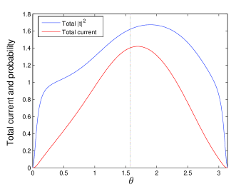
Figure 11: Total transmitted current (in units of $v$) and probability as a function of $\theta$ when both incident waves are present. We have taken $E=2$, $\lambda=1$, $V_{0}=1$, and $L=1$.

Figures 12 (a), 12 (b) and 12 (c) show the conductance as a function of $V_{0}L/v$ for different values of $\lambda$ and $L$. While we do not see appreciable oscillations in the conductance if $L$ and $\lambda$ are small, more and more oscillations become visible when $L$ becomes large and $\lambda$ approaches $E$.

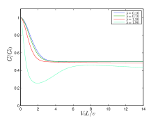
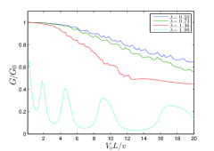
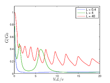
Figure 12: Conductance versus $V_{0}L/v$ for (a) different values of $\lambda$ and $L=1$, (b) different values of $\lambda$ and $L=10$, and (c) different values of $L$ and $\lambda=1.99$. We have taken $E=2$.

VI.2 Currents at top and bottom surfaces

We have again studied the transmitted currents and conductances on the top and bottom surfaces separately. We find that, just like the case of a potential barrier, the currents in either of the surfaces can take negative values for certain values of $\theta$ when only one incident wave is present. When both incident waves are present, we find that the current is always positive on both the surfaces.

The conductances at the top and bottom surfaces as a function of $V_{0}L/v$ are shown in Fig. 13 for two values of $\lambda$. Figure 13 (a) shows that when the coupling $\lambda$ is small, the bottom surface (which has no magnetic barrier) conducts almost the same current for different values of the barrier strength $V_{0}$, while the current at the top current decreases quickly as $V_{0}$ increases. When the coupling $\lambda$ has a value close to the energy $E$ (Fig. 13 (b)), the current at the top and bottom surfaces mix producing a more complex behavior. The current at the bottom surface decreases up to about $V_{0}L/v=2$ beyond which it increases and reaches a constant. The current at the top surface decreases up to about $V_{0}L/v=1$ where it is negative; beyond that value it increases and eventually reaches a constant value of zero. We note that this nonmonotonic variation with $V_{0}L/v$ occurs only when the barrier width is substantial; in contrast, the behavior is monotonic for a $\delta$-function magnetic barrier (Fig. 4) or when the width is $0.4$ (Fig. 12 (c)).

Finally, we present plots of the transmitted spin current, similar to the case of a potential barrier. In Fig. 14, we show the total spin current as a function of $V_{0}L/v$ when both incident waves are present. We do not see any oscillations in the spin current for the values of $\lambda$ and $L$ chosen in this figure. Indeed Fig. 14 looks very similar to Fig. 5 which showed the total spin current for a $\delta$-function magnetic barrier.

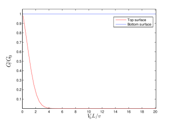
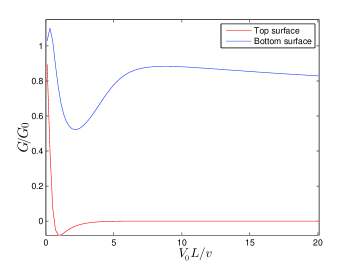
Figure 13: Conductances at the top and bottom surfaces versus $V_{0}L/v$ for (a) a small value of $\lambda=0.01$ and (b) a value of $\lambda=1.9$ close to $E$. We have taken $E=2$ and $L=1$.

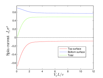
Figure 14: Total spin current (in units of $v$) as a function of $V_{0}L/v$ when both incident waves are present, $E=2$, $\lambda=1$, and $L=1$.

VI.3 Magnetic barrier with other orientations of magnetization

We have so far studied the effects of a magnetic barrier in which the magnetization points along the $x$-direction. We will now discuss briefly what happens if the magnetization points along the $y$- or $z$-direction. To obtain a qualitative understanding of these two cases, let us consider a $\delta$-function magnetic barrier on the top surface similar to the situation studied in Secs. IV.3 and IV.4. If the magnetization points along the $y$-direction, we get a Hamiltonian and a matching condition on the top surface given by

$$H~{}=~{}v(-i\sigma^{x}\partial_{y}+i\sigma^{y}\partial_{x})~{}+~{}c~{}\delta(x)~{}\sigma^{y},$$ (76)

and

$$\psi_{x\to 0^{+}}~{}=~{}e^{i(c/v)}\psi_{x\to 0^{-}}.$$ (77)

This resembles the matching condition given in Eq. (40) for a $\delta$-function potential barrier in the sense that $\psi_{x\to 0^{+}}$ and $\psi_{x\to 0^{-}}$ are related by a unitary transformation. We find numerically as well that the dependence of the conductance on the various parameters is similar to the case of a $\delta$-function potential barrier. For instance, in both cases, the conductance oscillates with increasing barrier strength $c$ as in Fig. 2.

On the other hand, if the magnetization points along the $z$-direction, the Hamiltonian and matching condition on the top surface are given by

$$H~{}=~{}v(-i\sigma^{x}\partial_{y}+i\sigma^{y}\partial_{x})~{}+~{}c~{}\delta(x)~{}\sigma^{z},$$ (78)

and

$$\psi_{x\to 0^{+}}~{}=~{}e^{-(c/v)\sigma^{x}}\psi_{x\to 0^{-}}.$$ (79)

This resembles the matching condition given in Eq. (51) for a $\delta$-function magnetic barrier with magnetization pointing in that the $x$-direction in that the matrix connecting $\psi_{x\to 0^{+}}$ to $\psi_{x\to 0^{-}}$ is not unitary. Numerical calculations show that the dependence of the conductance on the various parameters is indeed similar to the case of a $\delta$-function magnetic barrier with magnetization in the $x$-direction. In both cases, the conductance becomes small and saturates at a nonzero value with increasing $c$ as in Fig. 4.

Thus the effects of a magnetic barrier with magnetization along the $y$- and $z$-directions are, respectively, similar to a potential barrier and to a magnetic barrier with magnetization in the $x$-direction.

VII Discussion

In this work, we have studied a three-dimensional topological insulator in which the states at the top and bottom surfaces are coupled to each other, with the coupling being characterized by an energy scale $\lambda$. For each value of the energy and surface momentum, there are two possible states which are linear combinations of states at the top and bottom surfaces. We have considered two types of barriers applied to the top surface, a potential barrier and a magnetic barrier. We have studied the transmitted currents and conductances as functions of various parameters of the system: the angle of incidence $\theta$ of the incident waves, the coupling $\lambda$, and the strength of the barrier $V_{0}$. We also studied the transmitted currents at the top and bottom surfaces separately which gives a clearer picture of the contributions from the two surfaces. Further, we have studied the transmitted spin currents at the two surfaces separately. We note that the qualitative features of many of the results obtained for barriers with finite widths can be analytically understood using models with $\delta$-function barriers.

The main results obtained for potential barriers are as follows. First, we have shown that the transmitted currents from the two possible incident waves as a function of the angle of incidence $\theta$ are symmetric about normal incidence ($\theta=\pi/2$). Moreover, the conductance $G/G_{0}$ is, expectedly, an oscillatory function of the barrier strength $V_{0}$. The difference of these oscillations from their single surface counterpart is that their period increases from $\pi$ to $2\pi$ (in dimensionless units) as we increase the coupling $\lambda$. The conductance at the peaks of these oscillations reaches almost unity, independent of the value of $\lambda$, for specific values of the barrier potential $V_{0}$ thus demonstrating near-perfect transmission resonances. Second, for a fixed value of $V_{0}$, the conductance as a function of the coupling $\lambda$ decreases with increasing $\lambda$. Third, looking at the currents at the top and bottom surfaces separately, we find that when we send only one of the two possible incident waves, the currents can take negative values for a small range of values of $\theta$ close to glancing angles. This shows that due to the coupling $\lambda$ between the two surfaces, some current can tunnel from the top surface to the bottom surface or vice versa. However, the sum of the currents when both incident waves are present is always positive at both the surfaces. Fourth, the transmitted spin current (with spin component along the $\hat{y}$ direction) is observed to be always negative (positive) at the top (bottom) surface, but their sum is always positive. This is due to the opposite forms of spin-momentum locking on the two surfaces as mentioned after Eq. (7); an electron with positive energy and moving in the $+\hat{x}$ direction on the top (bottom) surface has a spin pointing in the $-\hat{y}$ ($+\hat{y}$) direction, respectively. We note that this allows the usage of these junctions as splitters of currents into two separate spin currents with opposite polarizations. These spin currents can be picked up by attaching spin-polarized metallic leads to the two surfaces.

Next we summarize our main results for magnetic barriers. First, for a barrier in which the magnetization points along the $\hat{x}$ direction, the transmitted current as a function of the angle of incidence $\theta$ is not symmetric about normal incidence ($\theta=\pi/2$), unlike the case of a potential barrier. This is because the magnetic barrier breaks the symmetry $\theta\to\pi-\theta$. Moreover, the normalized conductance $G/G_{0}$ does not oscillate but decreases and reaches a constant value as the barrier strength $V_{0}$ increases, in contrast to the case of a potential barrier. Even for very large $V_{0}$, there is always a nonzero current due to the presence of the bottom surface. Second, the conductance decreases as a function of $\lambda$ for a given value of $V_{0}$. As $E\to\lambda$, the current goes to zero. Third, the currents at the top and bottom surfaces separately can again exhibit negative values near the glancing angles, for the same reasons as mentioned above. Finally, the transmitted spin currents have opposite signs on the top and bottom surfaces due to the spin-momentum locking as discussed above.

In this work, we have not considered the effects of disorder. In the limit of strong nonmagnetic disorder, where the mean free path of the Dirac electrons becomes less than the width of the potential or magnetic barrier, the effect of the disorder would have to be considered. This is, by itself, an interesting problem and could be a topic of future study. However, in this paper, we have concentrated on the other (ballistic) limit, where the mean free path of the Dirac electrons is much larger than the barrier width. In this weak disorder or “clean” limit, as also pointed out in Ref. fogler, in the context of two-dimensional Dirac electrons in graphene, the transmission is not significantly affected. Further, such systems with weak disorder are experimentally feasible; thus this limit is expected to have experimental relevance.

The experimental verification of our results would involve transport measurements in these systems. The best experimental set-up would involve four leads which separately connect to the top and bottom surfaces on the left and on the right of the barrier. One can then apply a common voltage to the two input leads on the left side from where the electrons are incident, and measure the currents individually at the two output leads on the right side where the electrons are transmitted. Apart from attaching the leads, one would also need to implement the potential and magnetic barriers for these experiments. The potential barriers can be implemented by putting gates across the top surface. For magnetic barriers, one would need to deposit a layer of magnetized material with magnetization along $\hat{x}$ on the top surface; such a strip will induce a magnetization on the region below it via the proximity effect and thus mimic the Hamiltonian of region $II$ mondal . The first experiment that we suggest involves attaching spin-polarized leads with opposite spin polarizations, along $-\hat{y}$ and $+\hat{y}$, at the top and bottom surfaces, respectively. This would allow one to pick up oppositely polarized spin currents as output for a generic charge current input in these junctions. We predict that a much smaller output current will be picked up if the spin-polarizations of the leads on the two surfaces are reversed (i.e., $+\hat{y}$ and $-\hat{y}$ at the top and bottom surfaces). Further, one can carry out a standard tunneling conductance measurement with these junctions in the presence of potential barriers. The period of the oscillations of these tunneling conductances as a function of the barrier strength (which could be tuned using the gate voltage on the top surface) would depend on $\lambda/E$. Although it would be difficult to tune $\lambda$, one can easily tune the incident electron energy $E$ and verify the change in the period of $G$ as a function of $\lambda/E$ predicted in this work.

In conclusion, we have studied the transport across a junction of a thin topological insulator whose top and bottom surface are connected by a coupling of strength $\lambda$ in the presence of either a potential or a magnetic barrier atop its top surface. We have shown that such junctions show conductance oscillations as a function of the potential barrier strength whose period can be tuned by varying $E$. For a magnetic barrier, the conductance approaches a finite nonzero value with increasing barrier strength. We find that the spin currents on the top and bottom surfaces of such junctions always have opposite polarizations. Consequently, they can act as splitters of a charge current into two oppositely oriented spin currents. We have suggested experiments to test our theory.

Acknowledgments

D.S. thanks DST, India for Project No. SR/S2/JCB-44/2010 for financial support.

References

- (1)
- (2) C. L. Kane and E. J. Mele, Phys. Rev. Lett. 95, 226801 (2005); ibid, Phys. Rev. Lett. 95, 146802 (2005).
- (3) B. A. Bernevig, T. L. Hughes, and S.-C. Zhang, Science 314, 1757 (2006); B. A. Bernevig and S.-C. Zhang, Phys. Rev. Lett. 96, 106802 (2006).
- (4) L. Fu, C. L. Kane, and E. J. Mele, Phys. Rev. Lett. 98, 106803 (2007); J. C. Y. Teo, L. Fu, and C. L. Kane, Phys. Rev. B 78, 045426 (2008).
- (5) J. E. Moore and L. Balents, Phys. Rev. B 75, 121306 (2007); R. Roy, Phys. Rev. B 79, 195322 (2009).
- (6) M. Z. Hasan and C. L. Kane, Rev. Mod. Phys. 82, 3045 (2010).
- (7) X.-L. Qi and S.-C. Zhang, Rev. Mod. Phys. 83, 1057 (2011).
- (8) Y. L. Chen, J. G. Analytis, J. H. Chu, Z. K. Liu, S. K. Mo, X. L. Qi, H. J. Zhang, D. H. Lu, X. Dai, Z. Fang, S.-C. Zhang, I. R. Fisher, Z. Hussain, Z. X. Shen, Science 325, 178 (2009).
- (9) T. Zhang, P. Cheng, X. Chen, J.-F. Jia, X. Ma, K. He, L. Wang, H. Zhang, X. Dai, Z. Fang, X. Xie, and Q.-K. Xue, Phys. Rev. Lett. 103, 266803 (2009).
- (10) D. Hsieh, D. Qian, L. Wray, Y. Xia, Y. S. Hor, R. J. Cava, and M. Z. Hasan, Nature (London) 452, 970 (2008).
- (11) D. Hsieh, Y. Xia, L. Wray, D. Qian, A. Pal, J. H. Dil, J. Osterwalder, F. Meier, G. Bihlmayer, C. L. Kane, Y. S. Hor, R. J. Cava, and M. Z. Hasan, Science 323, 919 (2009).
- (12) Y. Xia, D. Qian, D. Hsieh, L. Wray, A. Pal, H. Lin, A. Bansil, D. Grauer, Y. S. Hor, R. J. Cava, and M. Z. Hasan , Nature Physics 5, 398 (2009).
- (13) P. Roushan, J. Seo, C. V. Parker, Y. S. Hor, D. Hsieh, D. Qian, A. Richardella, M. Z. Hasan, R. J. Cava, and A. Yazdani, Nature (London) 460, 1106 (2009).
- (14) C.-X. Liu, X.-L. Qi, H. J. Zhang, X. Dai, Z. Fang, and S.-C. Zhang, Phys. Rev. B 82, 045122 (2010).
- (15) F. Zhang, C. L. Kane, and E. J. Mele, Phys. Rev. B 86, 081303(R) (2012), and Phys. Rev. Lett. 110, 046404 (2013).
- (16) O. Deb, A. Soori, and D. Sen, J. Phys. Condens. Matter 26, 315009 (2014).
- (17) D. Hsieh, Y. Xia, D. Qian, L. Wray, J. H. Dil, F. Meier, L. Patthey, J. Osterwalder, A. V. Fedorov, H. Lin, A. Bansil, D. Grauer, Y. S. Hor, R. J. Cava, and M. Z. Hasan, Nature (London) 460, 1101 (2009).
- (18) L. Fu and C. L. Kane, Phys. Rev. Lett. 100, 096407 (2008); A. R. Akhmerov, J. Nilsson, and C. W. J. Beenakker, Phys. Rev. Lett. 102, 216404 (2009); Y. Tanaka, T. Yokoyama, and N. Nagaosa, Phys. Rev. Lett. 103, 107002 (2009); J. Linder, Y. Tanaka, T. Yokoyama, A. Sudbo, and N. Nagaosa, Phys. Rev. Lett. 104, 067001 (2010).
- (19) D. Sen and O. Deb, Phys. Rev. B 85, 245402 (2012); Erratum, Phys. Rev. B 86, 039902(E) (2012).
- (20) C. Wickles and W. Belzig, Phys. Rev. B 86, 035151 (2012).
- (21) R. R. Biswas and A. V. Balatsky, Phys. Rev. B 83, 075439 (2011).
- (22) M. Alos-Palop, R. P. Tiwari, and M. Blaauboer, Phys. Rev. B 87, 035432 (2013).
- (23) M. Sitte, A. Rosch, E. Altman, and L. Fritz, Phys. Rev. Lett. 108, 126807 (2012).
- (24) V. M. Apalkov and T. Chakraborty, EPL 100, 17002 (2012), and EPL 100, 67008 (2012).
- (25) T. Habe and Y. Asano, Phys. Rev. B 88, 155442 (2013), and Phys. Rev. B 89, 115203 (2014).
- (26) S. Modak, K. Sengupta, and D. Sen, Phys. Rev. B. 86, 205114 (2012).
- (27) A. Soori, O. Deb, K. Sengupta, and D. Sen, Phys. Rev. B 87, 245435 (2013).
- (28) J. Nussbaum, T. L. Schmidt, C. Bruder, and R. P. Tiwari, Phys. Rev. B 90, 045413 (2014).
- (29) S. Mondal, D. Sen, K. Sengupta, and R. Shankar, Phys. Rev. Lett. 104, 046403 (2010); ibid, Phys. Rev. B 82, 045120 (2010).
- (30) Z. Wu, F. M. Peeters, and K. Chang, Phys. Rev. B 82, 115211 (2010); ibid, Applied Phys. Lett. 98, 162101 (2011).
- (31) A. A. Burkov and D. G. Hawthorn, Phys. Rev. Lett. 105, 066802 (2010); I. Garate and M. Franz, Phys. Rev. B 81, 172408 (2010).
- (32) K. Nomura and N. Nagaosa, Phys. Rev. B 82, 161401 (2010).
- (33) T. Yokoyama, J. Zang, and N. Nagaosa, Phys. Rev. B 81, 241410(R) (2010).
- (34) R. Ilan, F. de Juan, and J. E. Moore, Phys. Rev. Lett. 115, 096802 (2015).
- (35) N. Dai, Y.-F. Zhou, P. Lv, and Q.-F. Sun, Phys. Rev. B 98, 085422 (2018).
- (36) K. Moors, P. Schüffelgen, D. Rosenbach, T. Schmitt, T. Schäpers, and T. L. Schmidt, Phys. Rev. B 97, 245429 (2018).
- (37) Y.-F. Zhou, H. Jiang, X. C. Xie, and Q.-F. Sun, Phys. Rev. B 95, 245137 (2017).
- (38) W.-Y. Shan, H.-Z. Lu, and S.-Q. Shen, New J. Phys. 12, 043048 (2010).
- (39) A. A. Zyuzin, M. D. Hook, and A. A. Burkov, Phys. Rev. B 83, 245428 (2011).
- (40) M. M. Asmar, D. E. Sheehy, and I. Vekhter, Phys. Rev. B 97, 075419 (2018).
- (41) B. Seradjeh, J. E. Moore, and M. Franz, Phys. Rev. Lett. 103, 066402 (2009).
- (42) B. Seradjeh, Phys. Rev. B 86, 121101(R) (2012).
- (43) B. Zhou, H.-Z. Lu, R.-L. Chu, S.-Q. Shen, and Q. Niu, Phys. Rev. Lett. 101, 246807 (2008); H.-Z. Lu, W.-Y. Shan, W. Yao, Q. Niu, and S.-Q. Shen, Phys. Rev. B 81, 115407 (2010).
- (44) J. Linder, T. Yokoyama, and A. Sudbo, Phys. Rev. B 80, 205401 (2009).
- (45) R. Egger, A. Zazunov, and A. Levy Yeyati, Phys. Rev. Lett. 105, 136403 (2010).
- (46) A. Kundu, A. Zazunov, A. Levy Yeyati, T. Martin, and R. Egger, Phys. Rev. B 83, 125429 (2011).
- (47) A. Medhi and V. B. Shenoy, J. Phys. Condens. Matter 24, 355001 (2012).
- (48) A. Pertsova and C. M. Canali, New J. Phys. 16, 063022 (2014).
- (49) M. I. Katsnelson, K. S. Novoselov, and A. K. Geim, Nature Physics 2, 620 (2006).
- (50) M. M. Fogler, F. Guinea, and M. I. Katsnelson, Phys. Rev. Lett. 101, 226804 (2008).