$\mathcal{R}_{0}$ fails to predict the outbreak potential in the presence of natural-boosting immunity

Abstract.

Time varying susceptibility of host at individual level due to waning and boosting immunity is known to induce rich long-term behavior of disease transmission dynamics. Meanwhile, the impact of the time varying heterogeneity of host susceptibility on the shot-term behavior of epidemics is not well-studied, even though the large amount of the available epidemiological data are the short-term epidemics. Here we constructed a parsimonious mathematical model describing the short-term transmission dynamics taking into account natural-boosting immunity by reinfection, and obtained the explicit solution for our model. We found that our system show “the delayed epidemic”, the epidemic takes off after negative slope of the epidemic curve at the initial phase of epidemic, in addition to the common classification in the standard SIR model, i.e., “no epidemic” as $\mathcal{R}_{0}\leq 1$ or normal epidemic as $\mathcal{R}_{0}>1$. Employing the explicit solution we derived the condition for each classification.

1. Introduction

Modelling the transmission dynamics of infectious diseases and the estimation of its model parameters are essential to understand the transmission dynamics. Susceptible-infective-removed model, so-called SIR model is known to be the simplest model to describe the transmission dynamics [1, 9]. The SIR model describes transmission of pathogen from infective individuals to susceptible individuals and removing infective individuals from the targeted host population due to the establishment of immunity or death of host or host immigration. Due to the wide variation in the natural history of pathogen, many extended models from the basic SIR model have been proposed so far.

An important extension is the time-evolution of susceptibility against the infection with a pathogen. The basic SIR model describes that the host immunity perfectly protects the host from reinfection over time, then reinfection cannot occur forever. Meanwhile, reinfection events are observed frequently among many infectious diseases, e.g., Coronavirus [19], Respiratory syncytial virus [14], Tuberculosis [30] and Hepatitis C virus [29]. One of considerable mechanisms of reinfection is waning immunity. Decreased herd immunity by waning immunity of individuals induces re-emergence of epidemic, and boosting immunity by re-vaccination is required to control epidemics [4]. Another mechanism is imperfectness of immunity by an infection event. The booster dose of vaccine is required to establish the high enough immunity level to protect hosts from reinfection [28], this implies that the multiple exposures to the pathogen is required to establish the high enough immunity level. Moreover, the enhancement of susceptibility to reinfection is also observed among several infectious diseases [31, 23].

Epidemic models incorporating variable susceptibility of recovered individuals was formulated in the papers [21, 22] by Kermack and McKendrick. However, the authors did not obtain a clear biological conclusion [7, 17]. In [17, 16] the author performed stability analysis for the Kermack and McKendrick’s reinfection model formulated as a system of partial differential equations. The existence and bifurcation of the endemic equilibrium is analyzed in detail. Destabilization of the endemic equilibrium was shown to be possible for epidemic models with waning immunity [8, 15, 27]. Previous modeling studies showed that waning and natural-boosting immunity by exposure to the pathogens can trigger a counter-intuitive effect of vaccination [26]. It is suggested that waning immunity in vaccinated hosts can trigger backward bifurcation of the endemic equilibrium [2, 5, 25]. Estimating the vaccine effectiveness is essential to control epidemics, however, vaccine effectiveness reflects the complicated epidemiological dynamics which is scaled by waning and natural-boosting immunity, e.g., boosting and waning immunity can induce the periodic outbreak for the long-term behavior [3].

Compared to the long-term behavior, the short-term behavior with waning and boosting immunity is not well understood, although many field data of the short-term epidemics have been analyzed using the model without such waning and boosting immunity. As for short-term behavior, the dynamics with constant immune protection rate against reinfection has been studied so far while boosting and waning immunity change the immune protection rate. In [20] the author analyzed transient dynamics of a reinfection epidemic model, ignoring the demographic process in the model studied in [12]. In the model, reinfection of recovered individuals occurs, assuming that recovered individuals have suitable susceptibility to the disease. It was shown that the disease transmission dynamics qualitatively changes, when the basic reproduction number crosses the reinfection threshold.

In this paper, we constructed a mathematical model taking into account natural-boosting immunity. Since the time scale of waning immunity is relatively longer than transmission dynamics, e.g., minimal annual waning rate of immunity is $-2.9\%$ for rubella and $-1.6\%$ for measles [24], compared to the infectious periods, $11$ days for rubella [10] and $14$ days for measles [1], we here focus on only boosting immunity. Since boosting and waning immunity can induce periodic outbreak for the long-term behavior [3], complicated epidemic curve may be observed in the model for a short-term disease transmission dynamics. We here obtain an explicit solution for the number of infective individuals, consequently, we investigated how the short-term behavior of the transmission dynamics is influenced by boosting immunity. The shape of the short-term epidemic curve is analyzed in detail.

The paper is organized as follows. In Section 2 we formulate an epidemic model, taking into account natural-boosting immunity, by a nonlinear system of differential equations. The model includes the standard SIR epidemic model and the reinfection epidemic model studied in [20] as special cases. In Section 3 we study the disease transmission dynamics when the basic reproduction number, which is denoted by $\mathcal{R}_{0}$, exceeds one. The number of the epidemic curve is shown to be one, as is the case for the standard SIR epidemic model. In Section 3 we consider disease transmission dynamics when $\mathcal{R}_{0}\leq 1$. Here we show that epidemic occurs even if $\mathcal{R}_{0}\leq 1$, due to the enhancement of susceptibility of recovered individuals. We analyze the shape of the epidemic curve in detail. In Section 4, the final size relation is derived from the explicit solutions in the phase planes. In Section 6 we discuss our results for the future works.

2. An epidemic model with natural-boosting immunity

First of all let us introduce the epidemic model studied in [20]. In the model it is assumed that the infectious disease induces partial immunity. Denote by $S(t),\ I(t)$ and $R(t)$ the proportions of susceptible population, infective population and recovered population at time $t$, respectively. The partial immunity model is formulated as

(2.1a) $$S^{\prime}(t) =-\beta S(t)I(t),$$

(2.1b) $$I^{\prime}(t) =\beta S(t)I(t)+\beta\sigma R(t)I(t)-\gamma I(t),$$

(2.1c) $$R^{\prime}(t) =\gamma I(t)-\beta\sigma R(t)I(t).$$

The positive parameters $\beta$ and $\gamma$ are the transmission coefficient and the recovery rate, respectively. The parameter $\sigma$ is the relative susceptibility of recovered individuals, who have been infected at least once and have recovered from the infection. We obtain the standard SIR epidemic model, if $\sigma=0$, i.e., recovered individuals are completely protected from the infection.

In this paper the partial immunity model (2.1) is modified as follows. When a recovered individual is exposed to the force of infection, immunity is boosted with probability $1-\alpha$ so that one obtains permanent immunity to the disease, while one contracts the disease again with probability $\alpha$. The partial immunity model (2.1) is modified as

(2.2a) $$S^{\prime}(t) =-\beta S(t)I(t),$$

(2.2b) $$I^{\prime}(t) =\beta S(t)I(t)-\gamma I(t)+\beta\sigma\alpha I(t)R(t),$$

(2.2c) $$R^{\prime}(t) =\gamma I(t)-\beta\sigma I(t)R(t),$$

(2.2d) $$B^{\prime}(t) =\beta\sigma\left(1-\alpha\right)I(t)R(t)$$

with the following initial conditions

$$S(0)>0,\ I(0)>0,\ R(0)\geq 0,\ B(0)\geq 0,$$

$$S(0)+I\left(0\right)+R\left(0\right)+B\left(0\right)=1.$$

Here $B(t)$ denotes the proportion of population with permanent immunity at time $t$. We obtain the model (2.1) by $\alpha=1$ and the SIR model by $\alpha=0$. Throughout the paper, we assume the following two conditions

(2.3) $$0 <\sigma,$$

(2.4) $$0 <\alpha<1.$$

3. One epidemic peak for $\mathcal{R}_{0}>1$

We define the basic reproduction number by

$$\mathcal{R}_{0}:=\frac{\beta}{\gamma}\left(S\left(0\right)+\alpha\sigma R\left(0\right)\right).$$

The basic reproduction number is the expected number of secondary cases produced by one infective individual in the expected one infectious period, $\frac{1}{\gamma}$ in the initial phase of epidemic. Noting that both susceptible and recovered populations, which compose the initial host population, have susceptibility to the disease, we may call $\mathcal{R}_{0}$ the basic reproduction number, although $\mathcal{R}_{0}$ is conventionally called the effective reproduction number [18].

From (2.2a) and (2.2b) one obtains the following

(3.1) $$\frac{dI}{dS}=-\frac{\gamma}{\beta S}\left(\mathcal{R}(S,R)-1\right)$$

and

(3.2) $$\frac{dI(t)}{dt}=\gamma I(t)\left(\mathcal{R}(S(t),R(t))-1\right),$$

where

$$\mathcal{R}(S,R):=\frac{\beta}{\gamma}\left(S+\alpha\sigma R\right),\ S\geq 0,\ R\geq 0.$$

Noting that $\mathcal{R}\left(S(0),R(0)\right)=\mathcal{R}_{0}$, it is easy to see that

$$\mathcal{R}_{0}>1\Leftrightarrow I^{\prime}(0)>0,$$

$$\mathcal{R}_{0}=1\Leftrightarrow I^{\prime}(0)=0,$$

$$\mathcal{R}_{0}<1\Leftrightarrow I^{\prime}(0)<0,$$

i.e., if $\mathcal{R}_{0}>1$ then the epidemic curve initially grows, while if $\mathcal{R}_{0}<1$ then the epidemic curve initially decays.

First we show that $R(t)$ can be expressed in terms of $S(t)$.

Lemma 1.

It holds that

(3.3) $$R(t)=\frac{\gamma}{\sigma\beta}\left(1-\left(1-\frac{\sigma\beta}{\gamma}R\left(0\right)\right)\left(\frac{S\left(t\right)}{S\left(0\right)}\right)^{\sigma}\right),\ t\geq 0.$$

Proof.

Let us write $b$ for $\frac{\beta}{\gamma}$. Assume that $1-\sigma bR\left(0\right)\not=0$ holds. From the equations (2.2a) and (2.2c) we have

(3.4) $$\frac{dR}{dS}=-\frac{1-\sigma bR}{bS}.$$

Using the separation of variables, we obtain

(3.5) $$\left(\frac{S(t)}{S(0)}\right)^{\sigma}=\frac{1-\sigma bR\left(t\right)}{1-\sigma bR\left(0\right)},$$

thus (3.3) follows. It is easy to see that the equality in (3.3) also holds, if $1-\sigma bR\left(0\right)=0$. ∎

From Lemma 1 we have

(3.6) $$R(t)=r(S(t)),$$

where

(3.7) $$r(S):=\frac{\gamma}{\sigma\beta}\left(1-\left(1-\frac{\sigma\beta}{\gamma}R\left(0\right)\right)\left(\frac{S}{S(0)}\right)^{\sigma}\right),\ 0\leq S\leq S(0).$$

To analyze the epidemic curve, we study the function $\mathcal{R}(S,R)$ with $R=r\left(S\right)$. Let

$$\hat{\mathcal{R}}(S):=\mathcal{R}(S,r\left(S\right))$$

We then compute the first and second derivatives of $\hat{\mathcal{R}}$:

(3.8) $$\hat{\mathcal{R}}^{\prime}\left(S\right) =\frac{\beta}{\gamma}\left(1+\alpha\sigma r^{\prime}\left(S\right)\right).$$

(3.9) $$\hat{\mathcal{R}}^{\prime\prime}\left(S\right) =\frac{\beta\alpha\sigma}{\gamma}r^{\prime\prime}\left(S\right).$$

From the equation (3.4) in Lemma 1, it is easy to obtain the following result.

Lemma 2.

One has

(3.10) $$r^{\prime}(S) =-\frac{\gamma}{\beta}\left(1-\sigma bR(0)\right)\frac{S^{\sigma-1}}{S(0)^{\sigma}},$$

(3.11) $$r^{\prime\prime}(S) =\left(\sigma-1\right)\frac{1}{S}r^{\prime}(S).$$

Note that $r$ is a monotone function, thus $\hat{\mathcal{R}}$ has at most one extremum.

We now show the standard epidemic case if $\mathcal{R}_{0}>1$ holds.

Proposition 3.

Let us assume that $\mathcal{R}_{0}>1$ holds. Then

(3.12) $$\hat{\mathcal{R}}(0)=\alpha<1<\hat{\mathcal{R}}(S(0))=\mathcal{R}_{0}.$$

holds and there exists a unique root of

$$\hat{\mathcal{R}}(S)=1,\ 0<S<S(0).$$

Proof.

It is easy to see that (3.12) holds. First assume that $r^{\prime}(S)\geq 0$ for $0\leq S\leq S(0)$. Then, from (3.8), one can see that $\hat{\mathcal{R}}$ is an increasing function. Thus we obtain the conclusion. Next assume that $r^{\prime}(S)<0$ for $0\leq S\leq S(0)$. By Lemma 2, one sees that $\hat{\mathcal{R}}$ has at most one extremum for $0\leq S\leq S(0)$. Therefore, from (3.12), we obtain the conclusion. ∎

Then, from Proposition 3 and Lemma 10 in Appendix A, we obtain the following result.

Theorem 4.

Let us assume that $\mathcal{R}_{0}>1$ holds. Then there is a $t_{p}>0$ such that $I$ is monotonically increasing for $t\in\left(0,t_{p}\right)$ and monotonically decreasing for $t>t_{p}$. It holds $\lim_{t\to\infty}I(t)=0$.

4. Delayed epidemic for $\mathcal{R}_{0}\leq 1$

In the standard SIR model, when $\mathcal{R}_{0}\leq 1$ holds, then the epidemic curve monotonically decreases and infective population tends to $0$ eventually as time goes to infinity. The situation changes in the model with boosting immunity (2.2), due to the susceptibility of the recovered individuals. In particular, if $\sigma>1$ then there is a possible delayed outbreak as the recovered population increases which will induce the epidemic later even if $\mathcal{R}_{0}\leq 1$. The basic reproduction number, which characterizes the initial dynamics, is not a sufficient criterion to determine the outbreak due to the recovered population.

First let us consider a simple case that $\sigma\leq 1$ holds. We have the standard scenario: if $\mathcal{R}_{0}\leq 1$ then the epidemic does not occur. Subsequently we study the disease transmission dynamics when $\sigma>1$. We show that enhancement of susceptibility after the infection can induce an epidemic later.

4.1. $\sigma\leq 1$

We show that the infective population is monotonically decreasing for $t\geq 0$, similar to the SIR model, when $\mathcal{R}_{0}\leq 1$.

Proposition 5.

Let us assume that $\mathcal{R}_{0}\leq 1$ and $\sigma\leq 1$ holds. Then

$$\mathcal{\hat{R}}(S)\leq 1,\ 0\leq S\leq S(0).$$

Proof.

Note that

(4.1) $$\hat{\mathcal{R}}(0)=\alpha<1,\ \hat{\mathcal{R}}(S(0))=\mathcal{R}_{0}\leq 1$$

holds. Assume that $r^{\prime}(S)\geq 0$ for $0<S<S(0)$. Then $\hat{\mathcal{R}}$ is an increasing function, thus we obtain the conclusion. Next assume that $r^{\prime}(S)<0$ for $0<S<S(0)$. In this case one sees that

$$\lim_{S\downarrow 0}r^{\prime}(S)=-\infty\implies\lim_{S\downarrow 0}\hat{\mathcal{R}}^{\prime}(S)=-\infty.$$

By Lemma 2, one sees that $\hat{\mathcal{R}}$ has at most one minimum for $0\leq S\leq S(0)$. Therefore we obtain the conclusion. ∎

Then, from Propositions 5 and Lemma 10 in Appendix A, we obtain the following result.

Theorem 6.

Let us assume that $\mathcal{R}_{0}\leq 1$ and $\sigma\leq 1$ hold. Then $I$ is monotonically decreasing for $t\geq 0$. It holds $\lim_{t\to\infty}I(t)=0$.

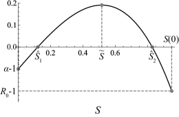
(a) Graph of $\hat{\mathcal{R}}(S)-1$

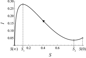
(b) Phase portrait of the solution $(I((t),S(t))$ in the $(I,S)$ plane

Figure 4.1. The graph of $\hat{\mathcal{R}}(S)-1$ for $0\leq S\leq S(0)$ is shown in (A). Here $\mathcal{R}_{0}\leq 1$ and $\sigma>1$. The parameters are chosen such that (4.4) and $\hat{\mathcal{R}}(\tilde{S})>1$ hold. The parametric curve $t\to(I(t),S(t))$ in the $(I,S)$ plane is plotted in (B). It is shown that $I$ has a local minima at $S=\hat{S}_{2}$ and local maxima at $S=\hat{S}_{1}$.

4.2. $\sigma>1$

In this subsection we consider the case that

(4.2) $$\mathcal{R}_{0}\leq 1,\ \sigma>1$$

hold. We show the following results for the graph of $\hat{\mathcal{R}}$.

Proposition 7.

Let us assume that $\mathcal{R}_{0}\leq 1$ and $\sigma>1$ hold.

1. If

   (4.3) $$\frac{\beta}{\gamma}\left(S(0)+\alpha\sigma^{2}R(0)\right)\geq\alpha\sigma$$

   then $\hat{\mathcal{R}}(S)\leq 1$ for $0\leq S\leq S(0)$.

2. If

   (4.4) $$\frac{\beta}{\gamma}\left(S(0)+\alpha\sigma^{2}R(0)\right)<\alpha\sigma$$

   then there is a unique maxima for $0<S<S(0)$ at $S=\tilde{S}$, where

   (4.5) $$\tilde{S}:=\left(\frac{\frac{\beta}{\gamma}S(0)}{\sigma\alpha\left(1-\frac{\sigma\beta}{\gamma}R(0)\right)}\right)^{\frac{1}{\sigma-1}}S(0)<S(0).$$

   Then

   1. If $\hat{\mathcal{R}}(\tilde{S})>1$ then there are two roots for $\hat{\mathcal{R}}(S)=1$ for $0<S<S(0)$. Denote the roots by $\hat{S}_{1}$ and $\hat{S}_{2}$ such that

      $$0<\hat{S}_{1}<\tilde{S}<\hat{S}_{2}<S(0),$$

      then

      $$\hat{\mathcal{R}}(S)\begin{cases}<1,&\hat{S}_{2}<S\leq S(0),\\ >1,&\hat{S}_{1}<S<\hat{S}_{2},\\ <1,&0<S<\hat{S}_{1}.\end{cases}$$

   2. If $\text{$\hat{\mathcal{R}}$}(\tilde{S})\leq 1$ then $\hat{\mathcal{R}}(S)\leq 1$ for $0\leq S\leq S(0)$.

Proof.

For $\sigma>1$ one sees that

$$\lim_{S\downarrow 0}r^{\prime}(S)=0\implies\lim_{S\downarrow 0}\hat{\mathcal{R}}^{\prime}(S)=\frac{\beta}{\gamma}>0.$$

From the monotonicity of $\hat{\mathcal{R}}^{\prime}$, if $\lim_{S\uparrow S(0)}\hat{\mathcal{R}}^{\prime}(S)>0$ then $\hat{\mathcal{R}}(S)\leq 1$ for $0\leq S\leq S(0)$ follows. Computing

$$\lim_{S\uparrow S(0)}\hat{\mathcal{R}}^{\prime}(S) =\frac{\beta}{\gamma}\left(1+\alpha\sigma r^{\prime}(S(0))\right)$$

$$=\frac{1}{S(0)}\left(\frac{\beta}{\gamma}\left(S(0)+\alpha\sigma^{2}R(0)\right)-\alpha\sigma\right),$$

one can see that (4.3) is equivalent to that $\lim_{S\uparrow S(0)}\hat{\mathcal{R}}^{\prime}(S)>0$ holds.

Next assume that (4.4) holds. Then

$$\lim_{S\uparrow S(0)}\hat{\mathcal{R}}^{\prime}(S)<0<\lim_{S\downarrow 0}\hat{\mathcal{R}}^{\prime}(S).$$

From the monotonicity of $\hat{\mathcal{R}}^{\prime},$ there is a unique maxima for $0<S<S(0)$. Solving $\hat{\mathcal{R}}^{\prime}(S)=0$, we obtain $\tilde{S}$ given as in (4.5). It is now straightforward to obtain the statements (a) and (b). ∎

In Figure 4.1, we plot the graph of the function $\hat{\mathcal{R}}(S)-1$ for $0\leq S\leq S(0)$, where $\mathcal{R}_{0}\leq 1$ and $\sigma>1$. Parameters are fixed so that (4.4) and $\hat{\mathcal{R}}(\tilde{S})>1$ hold.

From Proposition 7 and Lemma 10 in Appendix A, we first obtain the result for the extinction of the disease.

Theorem 8.

Let us assume that $\mathcal{R}_{0}\leq 1$ and $\sigma>1$ holds. If either that

1. (4.3) holds, or

2. (4.4) and $\hat{\mathcal{R}}(\tilde{S})\leq 1$ hold,

then $I$ is monotonically decreasing for $t\geq 0$. It follows that $\lim_{t\to\infty}I(t)=0$.

Now it is assumed that (4.2) holds. If

$$\hat{\mathcal{R}}(\tilde{S})>1$$

holds, where $\tilde{S}$ is a root of

$$\hat{\mathcal{R}}^{\prime}(S)=0$$

and the existence is ensured by the condition (4.4), then $I(t)$ may attain a minimum and a maxima (see Figure 4.1). This implies that even if $\mathcal{R}_{0}\leq 1$, the epidemic curve may grow for a certain time interval, which we call delayed epidemic.

To determine if the delayed epidemic indeed occurs, we evaluate the minimum of $I(t)$ using the following expression for $I$ derived in Proposition 12 in Appendix A

(4.6) $$I(t)=I(0)+p(S(t))-\alpha q(R(t)),\ t\geq 0,$$

where

$$p(S) :=\left(S(0)-S\right)+\frac{\gamma}{\beta}\ln\left(\frac{S}{S(0)}\right),$$

$$q(R) :=\frac{\gamma}{\sigma\beta}\ln\left(\frac{1-\frac{\sigma\beta}{\gamma}R}{1-\frac{\sigma\beta}{\gamma}R(0)}\right)+\left(R-R(0)\right).$$

Substituting (3.6) into (4.6), $I(t)$ can be expressed in terms of $S(t)$ as follows

$$I(t)=I(0)+p(S(t))-\alpha q(r(S(t)),\ t\geq 0.$$

See also Figure 4.1 (B) for the phase portrait in the $(I,S)$-plane.

Theorem 9.

Let us assume that $\mathcal{R}_{0}\leq 1$ and $\sigma>1$ holds. Furthermore, assume that (4.4) and

$$\hat{\mathcal{R}}(\tilde{S})>1$$

hold.

1. If $I(0)+p(\hat{S}_{2})-\alpha q(r(\hat{S}_{2}))\leq 0$, then $I$ is monotonically decreasing for $t\geq 0$.

2. If $I(0)+p(\hat{S}_{2})-\alpha q(r(\hat{S}_{2}))>0$, then there is an interval $\left[t_{1},t_{2}\right]$ such that $I$ increases for $t_{1}\leq t\leq t_{2}$ and decreases for $0\leq t\leq t_{1}$ and $t_{2}\leq t$.

It follows that $\lim_{t\to\infty}I(t)=0$.

Proof.

One sees that $I$ has a local maxima and minima with respect to $t$ and $S$, where $\hat{\mathcal{R}}(S)=1$ holds (see 3.1 and 3.2). $I$ has a local minima at $S=\hat{S}_{2}\in\left(\tilde{S},S(0)\right)$ and $I$ is increasing for $\hat{S}_{2}\leq S\leq S(0)$ (see Figure 4.1 (B)). Noting that $I(t)>0$ for $t\geq 0$ and that $S$ is a decreasing function with respect to $t$, $I(0)+p(\hat{S}_{2})-\alpha q(r(\hat{S}_{2}))\leq 0$ implies that $I$ is monotonically decreasing for $t\geq 0$. On the other hand, if $I(0)+p(\hat{S}_{2})-\alpha q(r(\hat{S}_{2}))>0$ then $I$ is monotonically increasing for $S<\hat{S}_{1}$, decreasing for $\hat{S}_{1}<S<\hat{S}_{2}$ and then increasing for $\hat{S}_{2}<S$. There exist $t_{1}$ and $t_{2}$ such that $S(t_{1})=\hat{S}_{2}$ and $S(t_{2})=\hat{S}_{1}$. Thus we obtain the conclusion. From Lemma 10 in Appendix A it follows that $\lim_{t\to\infty}I(t)=0$. ∎

Thus the model has three different transmission dynamics: no epidemic, normal epidemic and delayed epidemic as illustrated in Figure 4.2. Figure 4.3 shows parameter regions for the three different disease transmission dynamics. The region for the delayed epidemic become larger with respect to the initial condition of $I$ and the susceptibility $\sigma$. Since the initial condition of $I$ is involved in the condition of Theorem 9, the initial condition qualitatively changes the epidemic curve, see Figure 4.4: delayed epidemic is induced by a large initial condition.

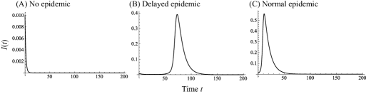
Figure 4.2. Examples of three types of epidemic curve. (A) shows no epidemic case, (B) shows delayed epidemic, and (C) shows normal epidemic, respectively. Parameters were set as $\mathcal{R}_{0}=0.4$ for (A), $0.8$ for (B), and $1.2$ for (C), other parameter values are identical between (A), (B) and (C): $\alpha=0.9,\>\sigma=5,\ S(0)=0.99,\>I(0)=0.01$, and $R(0)=B(0)=0$.

Figure 4.3. The dependency of epidemic type on $\mathcal{R}_{0}$ and $\alpha$ for several $\sigma$ and $I\left(0\right)$. White are denotes “no epidemic”, light gray area denotes “delayed epidemic”, and gray area denotes “normal epidemic”, respectively.

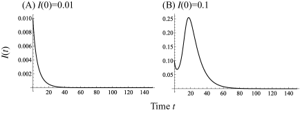
Figure 4.4. The initial condition for $I$ changes the disease transmission dynamics. Here parameters are chosen as $\beta=0.8,\ \gamma=1,\ \alpha=0.9,\ \sigma=3$. $R(0)=B(0)=0$. (A) shows no epidemic for $I(0)=0.1$ while (B) shows delayed epidemic for $I(0)=0.01$.

Consider a special case that $R\left(0\right)\to 0$. The basic reproduction number is given as

$$\mathcal{R}_{0}=\frac{\beta}{\gamma}S(0).$$

The conditions (4.4) becomes

$$\mathcal{R}_{0}<\sigma\alpha$$

and $\tilde{S}=\left(\frac{\mathcal{R}_{0}}{\sigma\alpha}\right)^{\frac{1}{\sigma-1}}S(0).$ If $\mathcal{\hat{R}}(\tilde{S})>1$ holds, then the delayed epidemic may occur.

5. Final epidemic size

Let

$$\left(S(\infty),I(\infty),R(\infty),B(\infty)\right)=\lim_{t\to\infty}\left(S(t),I(t),R(t),B(t)\right).$$

It follows that $I(\infty)=0$. From the relations (A.3), (3.3) and (A.4), one sees that $(S(\infty),R(\infty),B(\infty))$ satisfy the following equations

(5.1) $$0 =I(0)+p(S\left(\infty\right))-\alpha q(R\left(\infty\right)),$$

(5.2) $$R(\infty) =r(S(\infty)),$$

(5.3) $$B(\infty) =B(0)-\left(1-\alpha\right)q(R(\infty)).$$

The final epidemic size is given by $R(\infty)+B(\infty)$, the number of individuals who infected at least once. From (5.1) and (5.2) we get the following equation

(5.4) $$0=I(0)+p(S\left(\infty\right))-\alpha q(r\left(S(\infty)\right)).$$

In Figure 5.1, we plot $R(\infty)+B(\infty)=1-S(\infty),\ R(\infty)$ and $B(\infty)$ with respect to $\mathcal{R}_{0}$.

Numerically we observe that $R(\infty)$ is not monotone with respect to $\mathcal{R}_{0}$. Small $\mathcal{R}_{0}$ allows the increase of $R(\infty)$, on the other hand, does not contribute to the increase of $B(t)$, the outbreak ends before the transition from $R(t)$ to $B(t)$ via $I(t)$ occurs among most $R(t)$. Increase of $\mathcal{R}_{0}$ contributes the transition from $R(t)$ to $B(t)$, consequently, $R(\infty)$ decreases. Despite of non-monotnic relation of $R(\infty)$ with respect to $\mathcal{R}_{0}$, $R(\infty)+B(\infty)$ is likely to increase monotonically with the increase of $\mathcal{R}_{0}$ as shown in Figure 5.1.

When $\alpha=0$ we obtain the standard SIR setting. Letting $I(0)\to 0$ and $S(0)\to 1$, the basic reproduction number is given as $\mathcal{R}_{0}=b$. In this case, from (5.1), we obtain the well known final size relation

$$0=\left(1-S\left(\infty\right)\right)+\frac{1}{\mathcal{R}_{0}}\ln\left(S\left(\infty\right)\right),$$

see e.g. [9, 18].

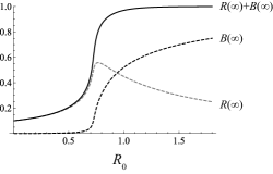
Figure 5.1. Final epidemic size with respect to $\mathcal{R}_{0}$. Initial conditions are fixed as $S(0)=0.9,\ I(0)=0.1,\ R(0)=B(0)=0$. Parameters are fixed as $\sigma=2,\ \alpha=0.8$.

6. Discussion

In this paper we study a disease transmission dynamics model incorporating natural-boosting immunity. Our modelling approach describing boosting immunity covers not only the standard transmission dynamics but also an interesting dynamics, delayed epidemic. Delayed epidemic shows negative slope at the initial phase of epidemic, thus, the estimation of $\mathcal{R}_{0}$ using the initial slope of epidemic is difficult to capture the actual epidemic coming later. We derive the condition for a delayed epidemic through deriving the analytic transient solution of $I(t)$.

Delayed epidemic, which is illustrated in Figures 4.2 and 4.4, occurs due to the enhancement of susceptibility of the recovered population (i.e., $\sigma>1$). For example, antibody dependent enhancement can enhance the viral replication within the host body, consequently, the host susceptibility can be enhanced at the time of reinfection [32]. In Theorem 9 we formulate a condition for the delayed epidemic. One of the necessary condition for the delayed epidemic is (4.4) in Proposition 7. The condition (4.4) is necessary for increasing of the epidemic curve and is related to increasing of the effective susceptible population, which is defined as

$$L(t):=S(t)+\alpha\sigma R(t).$$

Since it holds that

$$L^{\prime}(0) =S^{\prime}(0)+\alpha\sigma R^{\prime}(0)$$

$$=\gamma I(0)\left(-bS(0)+\alpha\sigma\left(1-b\sigma R(0)\right)\right),$$

one can see that

$$L^{\prime}(0)>0 \Leftrightarrow bS(0)<\sigma\alpha\left(1-b\sigma R(0)\right),$$

where $b=\frac{\beta}{\gamma}$. Therefore, increasing of the effective susceptible population at the initial time is necessary for the delayed epidemic and may induce the delayed epidemic even if $\mathcal{R}_{0}\leq 1$ holds.

We remark that $\mathcal{R}_{0}$ cannot measure the outbreak potential of “delayed epidemic”. In principe, $\mathcal{R}_{0}$ is derived based on the linearized system at the the initial disease transmission dynamics. The linearized system at the the initial phase does not provide enough information to predict the delayed epidemic. Similar phenomena can be observed in epidemic models that show backward bifurcation of the endemic equilibrium [2, 5, 13, 18, 25]. In those studies it is shown that there is a stable endemic equilibrium even if the basic reproduction number is less than unity. Differently from those models, the short-term disease transmission dynamics model have many equilibria, which are associated to the zero eigenvalue. Our study illustrates that, in the short-term disease transmission dynamics, the outbreak potential shall be carefully examined, using the transient solution.

We also observed the reinfection threshold like behavior [12, 20, 17] (see Figure 5.1). In the extreme case that the initial population is composed of only $I(0)$ and $R(0)$ ($S(0)=B(0)=0$), $\mathcal{R}_{0}=\frac{\beta}{\gamma}\alpha\sigma R\left(0\right)=1$ is shown to be the threshold for the outbreak, which amounts to the concept of the reinfection threshold. Differently from the models studied in [12, 20, 17], our model has the full protection compartment $B$. We here found that reinfection threshold is not a sufficient criterion for the outbreak if the initial population is composed of $S(0),I(0),R(0)$ and $B(0)$ (gray area shown in Figure 5.1).

$\mathcal{R}_{0}$ can be estimated from the final epidemic size. It should be noted that $\mathcal{R}_{0}$ can be overestimated if the model neglects the boosting immunity. Figure 6.1 shows the estimated $\mathcal{R}_{0}$ using a fixed final epidemic size $=0.5$ with varied $\alpha$ and $\sigma$, our model is equivalent with a standard SIR model when $\alpha=0$ or $\sigma=0$. If boosting and waning immunity are introduced, $\alpha>0$ or $\sigma>0$, the estimated $\mathcal{R}_{0}$ is always lower than it using the standard epidemic model, $\alpha=0$ or $\sigma=0$. To estimate the precise $\mathcal{R}_{0}$ from the final epidemic size, the appropriate modelling with respect to boosting and waning immunity is required.

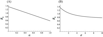
Figure 6.1. $\mathcal{R}_{0}$ derived from a given final epidemic size, $R(\infty)+B(\infty)=0.5$ with varied $\alpha$ and $\sigma$. When $\alpha=0$ or $\sigma=0$ the boosting and waning immunity do not occur (the standard SIR model). The initial conditions are fixed as $S(0)=0.99,\ I(0)=0.01,\ R(0)=B(0)=0$. Parameters are fixed as $\sigma=3$ for (A) and $\alpha=0.5$ for (B).

The time series data of the reported $I(t)$ is used to estimate the epidemiological parameters. However, the reported $I(t)$ can be biased by reporting biases and asymptomatic cases. Serological surveillance can collect the data which is less likely to suffer from such biases. Our analytical results allows the real-time estimation of $I(t)$ using the field data obtained by sero-surveillance. Since $I(t)$ can be implicitly determined from $R(t)+B(t)$ in our model. $1-(R(t)+B(t))=S(t)+I(t)$ and $I(t)$ is a function of $S(t)$, then $I(t)$ can be derived from $R(t)+B(t)$. If $R(t)+B(t)$ is collected by serological study, $I(t)$ can be estimated.

Our mathematical model describing natural-boosting immunity has a limitation; we described step-wise level of boosting immunity, i.e., $R$ has susceptibility $\sigma$ to the infectious disease while $B$ has a complete protection against reinfection. This setting is suitable for the infectious diseases such that the multiple infections can establish drastic increase of the immunity level. On the other hand, to describe gradual change of the immunity level resulted from boosting and waning immunity, the several classes of $R$ with varied immune protection level are required.

Acknowledgement

The first author was supported by JSPS Grant-in-Aid for Young Scientists (B) 16K20976 of Japan Society for the Promotion of Science. The second author was supported by PRESTO, Japan Science and Technology Agency, grant number JPMJPR15E1, and JSPS Grant-in-Aid for Young Scientists (B) 15K19217 of Japan Society for the Promotion of Science.

Appendix A Disease transmission dynamics

For simplicity, we write $b$ for $\frac{\beta}{\gamma}$.

Lemma 10.

There exist $\lim_{t\to\infty}S(t),\ \lim_{t\to\infty}I(t),\ \lim_{t\to\infty}R(t)$ and $\lim_{t\to\infty}B(t)$. It holds that

(A.1) $$\lim_{t\to\infty}I(t)=0.$$

Proof.

One easily sees that $S,\ R$ and $B$ are respectively monotone bounded functions. Specifically $S$ is a monotone decreasing function, while $B$ is a monotone increasing function. Therefore, $S,\ R$ and $B$ tend to some constants. Since $S(t)+I(t)+R(t)+B(t)=1$ holds for $t\geq 0$, $\lim_{t\to\infty}I(t)$ also exists. We now claim that (A.1) holds. From (2.2a), (2.2b) and (2.2c) one has

$$S^{\prime}(t)+I^{\prime}(t)+\alpha R^{\prime}(t)=-\gamma\left(1-\alpha\right)I(t).$$

Suppose that $\lim_{t\to\infty}I(t)>0$. Integrating the above equation, we derive a contradiction. Hence (A.1) holds. ∎

We now introduce the following lemma.

Lemma 11.

One has

(A.2) $$\int_{S(0)}^{S(t)}\frac{\sigma r(S)}{S}dS= \frac{1}{\sigma b}\ln\left(\frac{1-\sigma bR(t)}{1-\sigma bR(0)}\right)+\left(R(t)-R(0)\right),\ t\geq 0.$$

Proof.

We compute

$$\int\frac{\sigma r(S)}{S}dS= \sigma\int\frac{1}{S}\left[\frac{1}{\sigma b}\left(1-\left(1-\sigma bR(0)\right)\left(\frac{S}{S(0)}\right)^{\sigma}\right)\right]dS$$

$$= \frac{1}{b}\left[\int\frac{1}{S}dS-\left(1-\sigma bR(0)\right)\int\left(\frac{S}{S(0)}\right)^{\sigma}\frac{1}{S}dS\right].$$

First we have

$$\int_{S(0)}^{S(t)}\frac{1}{S}dS=\ln\left(\frac{S(t)}{S(0)}\right).$$

From (3.5) and (3.4) in the proof of Lemma 1 we get

$$\int\left(\frac{S}{S(0)}\right)^{\sigma}\frac{1}{S}dS =-b\int\left(\frac{1-\sigma bR}{1-\sigma bR(0)}\right)\frac{1}{1-\sigma bR}dR$$

$$=-b\frac{1}{1-\sigma bR(0)}\int dR.$$

Therefore, we get

$$\int_{S(0)}^{S(t)}\left(\frac{S}{S(0)}\right)^{\sigma}\frac{1}{S}dS=-b\frac{1}{1-\sigma bR(0)}\left(R(t)-R(0)\right).$$

Then

$$\int_{S(0)}^{S(t)}\frac{\sigma r(S)}{S}dS=\frac{1}{b}\ln\left(\frac{S(t)}{S(0)}\right)+\left(R(t)-R(0)\right).$$

From (3.5) in the proof of Lemma 1,

$$\ln\left(\frac{S(t)}{S(0)}\right)=\frac{1}{\sigma}\ln\left(\frac{1-\sigma bR(t)}{1-\sigma bR(0)}\right).$$

Finally we thus obtain (A.2). ∎

Then we show explicit expressions for $I$ and $B$ in terms of $S$ and $R$.

Proposition 12.

One has that

$$I(t)= I(0)+\left(S(0)-S(t)\right)+\frac{1}{b}\ln\left(\frac{S(t)}{S(0)}\right)$$

(A.3) $$-\alpha\left\{\frac{1}{\sigma b}\ln\left(\frac{1-\sigma bR(t)}{1-\sigma bR(0)}\right)+\left(R(t)-R(0)\right)\right\},$$

(A.4) $$B(t)= B(0)-\left(1-\alpha\right)\left\{\frac{1}{\sigma b}\ln\left(\frac{1-\sigma bR(t)}{1-\sigma bR(0)}\right)+\left(R(t)-R(0)\right)\right\}.$$

for $t\geq 0$.

Proof.

From (2.2a) and (2.2b) we have

(A.5) $$\frac{dI}{dS}=-1+\frac{1}{bS}-\alpha\sigma\frac{R}{S}.$$

We use the separation of variables to obtain (A.3). Using (A.2) in Lemma 11 one obtains

$$\int_{S(0)}^{S(t)}\left(\frac{1}{bS}-\alpha\sigma\frac{r(S)}{S}\right)dS=\frac{1}{b}\ln\left(\frac{S(t)}{S(0)}\right)-\alpha\left\{\frac{1}{\sigma b}\ln\left(\frac{1-\sigma bR(t)}{1-\sigma bR(0)}\right)+\left(R(t)-R(0)\right)\right\}.$$

Therefore we get (A.3). Next from (2.2a) and (2.2b) we have

(A.6) $$\frac{dB}{dS}=-\left(1-\alpha\right)\sigma\frac{R}{S}$$

Using (A.2) in Lemma 11, one obtains (A.4). ∎

References

- [1] R.M. Anderson, R.M. May, Infectious diseases of humans: dynamics and control, Vol. 28. Oxford: Oxford University Press, 1992
- [2] J. Arino, C. C. McCluskey, P. van den Driessche, Global results for an epidemic model with vaccination that exhibits backward bifurcation, SIAM J. Appl. Math., 64 (1) (2003) 260–276.
- [3] N. Arinaminpathy, J. S. Lavine, B. T. Grenfell, Self-boosting vaccines and their implications for herd immunity, PNAS, 109 (49) (2012) 20154-20159.
- [4] M.V. Barbarossa, A. Denes, G. Kiss, Y. Nakata, G. Röst, Zs. Vizi, Transmission dynamics and final epidemic size of Ebola Virus Disease outbreaks with varying interventions, PLOS ONE, 10 (7) (2015): e0131398.
- [5] F. Brauer, Backward bifurcations in simple vaccination models, J. Math. Anal. Appl. 298 (2) (2004) 418–431.
- [6] O. Diekmann, J. A. P. Heesterbeek, J. A. J. Metz, On the definition and the computation of the basic reproduction ratio in models for infectious diseases in heterogeneous populations, J. Math. Biol. 28 (4) (1990) 365–382.
- [7] O. Diekmann, J. A. P. Heesterbeek, J. A. J. Metz, The legacy of Kermack and McKendrick, Epidemic Models: Their Structure and Relation to Data. (D. Mollison, ed.) (1995) 95-115.
- [8] O. Diekmann, R. Montijn, Prelude to Hopf bifurcation in an epidemic model: analysis of a characteristic equation associated with a nonlinear Volterra integral equation, J. Math. Biol. 14 (1) (1982) 117–127.
- [9] O. Diekmann, H. Heesterbeek, T. Britton, Mathematical tools for understanding infectious disease dynamics, Princeton University Press, 2012.
- [10] W.J. Edmunds, O.G. Van de Heijden, M. Eerola, N. J. Gay, Modelling rubella in Europe, Epidemiology and Infection, 125 (03) (2000) 617-634.
- [11] P. van den Driessche, J. Watmough, Reproduction numbers and sub-threshold endemic equilibria for compartmental models of disease transmission, Mathematical Biosciences, 180 (1) (2002) 29-48.
- [12] M.G.M. Gomes, L.J. White, G.F. Medley, Infection, reinfection, and vaccination under suboptimal immune protection: epidemiological perspectives, J. Theor. Biol., 228 (4) (2004) 539–549
- [13] D. Greenhalgh, O. Diekmann, M. C. M de Jong, Subcritical endemic steady states in mathematical models for animal infections with incomplete immunity, Mathematical Biosciences 165 (1) (2000) 1-25.
- [14] C. Hall, E. Walsh, C. Long, K. Schnabel, Immunity to and frequency of reinfection with respiratory syncytial virus. The Journal of Infectious Diseases, 163 (4)(1991) 693–698
- [15] H.W. Hethcote, H.W. Stech, P. van den Driessche, Nonlinear oscillations in epidemic models, SIAM J. Appl. Math. 40 (1981) 1–9.
- [16] H. Inaba, Kermack and McKendrick revisited: the variable susceptibility model for infectious diseases, J. J. Ind. Appl. Math. 18 (2) (2001) 273–292.
- [17] H. Inaba, Endemic threshold analysis for the Kermack-McKendrick reinfection model, Josai Math. Mono. 9 (2016) 105–133.
- [18] H. Inaba, Age-structured population dynamics in demography and epidemiology, Springer, 2017
- [19] D. Isaacs, D. Flowers, J. R. Clarke, H. B. Valman, M. R. MacNaughton, Epidemiology of coronavirus respiratory infections, Archives of Disease in Childhood, 58 (7) (1983) 500–503.
- [20] G. Katriel, Epidemics with partial immunity to reinfection, Math. Biosci., 228 (2) (2010) 153–159
- [21] W.O. Kermack, A.G. McKendrick, Contributions to the mathematical theory of epidemics-II. The problem of endemicity. Proceedings of the Royal Society, 138A (1932), 55–83; Reprinted in Bull. Math. Biol., 53, No.1/2 (1991) 57–87.
- [22] W.O. Kermack, A.G. McKendrick, Contributions to the mathematical theory of epidemics-III. Further studies of the problem of endemicity. Proceedings of the Royal Society, 141A (1933), 94–122; Reprinted in Bull. Math. Biol., 53, No.1/2 (1991), 89–118
- [23] R. Kohlmann et al., Serological evidence of increased susceptibility to varicella-zoster virus reactivation or reinfection in natalizumab-treated patients with multiple sclerosis, Multiple Sclerosis J., 21 (14) (2015) 1823–1832.
- [24] J.R. Kremer, F. Schneider, C.P. Muller, Waning antibodies in measles and rubella vaccinees-a longitudinal study, Vaccine 24 (14) (2006) 2594–2601.
- [25] C.M. Kribs-Zaleta, J.X. Velasco-Hernandez, A simple vaccination model with multiple endemic states, Math. Biosci. 164 (2) (2000) 183–201.
- [26] J.S. Lavine, A. A. King, O. N. Bjørnstad, Natural immune boosting in pertussis dynamics and the potential for long-term vaccine failure, PNAS, 108 (17) (2011) 7259–7264.
- [27] Y. Nakata, Y. Enatsu, H. Inaba, T. Kuniya, Y. Muroya, Y. Takeuchi, Stability of epidemic models with waning immunity, SUT J. Math. 50 (2) (2014) 205–245.
- [28] C.A. Siegrist, Vaccine immunology. Vaccines 5 (2008): 1725.
- [29] T.J.W. van de Laar, et al., Frequent HCV reinfection and superinfection in a cohort of injecting drug users in Amsterdam. J. Hepatology 51 (4) (2009) 667–674.
- [30] S. Verver, et al., Rate of reinfection tuberculosis after successful treatment is higher than rate of new tuberculosis, American J. Respiratory and Critical Care Medicine 171 (12) (2005) 1430–1435.
- [31] G. Wei, H. Bull, X. Zhou, H. Tabel, Intradermal infections of mice by low numbers of African trypanosomes are controlled by innate resistance but enhance susceptibility to reinfection, Journal of Infectious Diseases, 203 (3) (2011) 418–429.
- [32] S.S. Whitehead, J.E. Blaney, A.P. Durbin, B.R. Murphy, Prospects for a dengue virus vaccine. Nature Reviews Microbiology 5.7 (2007) 518–528.