Dynamics of conservative peakons in a system of Popowicz
L.E. Barnes and A.N.W. Hone111Currently on leave at the School of Mathematics and Statistics, University of New South Wales, Kensington NSW 2052, Australia. School of Mathematics, Statistics and Actuarial Science
Sibson Building, University of Kent
Canterbury CT2 ,
UK
Abstract
We consider a two-component Hamiltonian system of
partial differential equations
with quadratic nonlinearities introduced by Popowicz, which has the form
of a coupling between the Camassa-Holm and Degasperis-Procesi equations. Despite having reductions
to these two integrable partial differential equations, the Popowicz system itself is not integrable. Nevertheless,
as one of the authors showed with Irle, it admits
distributional solutions of peaked soliton (peakon) type, with the dynamics of
peakons being determined by a Hamiltonian system on a phase space of dimension .
As well as the trivial case of a single peakon (), the case is Liouville
integrable. We present the explicit solution for the two-peakon dynamics, and describe
some of the novel features of the interaction of peakons in the Popowicz system.
1 Introduction
For the past 25 years there has been a huge amount of interest
in partial differential equations (PDEs) which admit peaked soliton solutions, known as
peakons, with a discontinuous first derivative at the peaks.
This began with the work of Camassa and Holm [4], who found the integrable
PDE
(1.1)
in the context of shallow water wave theory. In fact this was a
rediscovery, since the integrability of the latter equation had already
been recognized in the work of Fokas and Fuchssteiner on
hereditary symmetries and recursion operators [13].
However, the pioneering contribution of Camassa and Holm was
their analysis of the remarkable properties of the solutions
of (1.1), and in particular the fact that in the absence
of linear dispersion () it
has multipeakon solutions of the form
(1.2)
as well
as displaying wave breaking, and also (for ) smooth solitons vanishing at spatial infinity.
The equation (1.1) with is the case of the 1-parameter family
(1.3)
introduced in [10] after it was shown that the case ,
identified by Degasperis and Procesi [9], is also integrable
(linear dispersion can always be removed by a combination of a shift const and a Galilean transformation).
With the inclusion of linear dispersion, the whole b-family
of equations (1.3) was subsequently derived via
shallow water approximations [11, 8].
All of the equations in the family have at least one Hamiltonian structure, given by
(1.4)
where (subject to appropriate modifications for )
(1.5)
and admit
multipeakon solutions of the form (1.2). However,
are the only values for which there is a
bi-Hamiltonian structure, and these
correspond to the integrable cases,
in the sense that the equation (1.3) has infinitely many local symmetries
for these values of alone [20].
Due to the discontinuous derivatives at the peaks, it is necessary to specify
in what sense (1.2) is a solution of (1.3). The shape of the peakons
corresponds to the fact that is the Green’s function of
the one-dimensional Helmholtz operator , so for peakons the quantity
is given by a sum of Dirac delta functions,
(1.6)
with support at each of the peak positions at time . Thus
it is necessary to interpret (1.3) as an equation for distributions. The problem
is then how to make sense of the nonlinear terms, which include products of distributions
with common support. An ad hoc solution to this problem is to interpret the product as
being , where
(1.7)
is the average of the left and right limits. However, a more satisfying
solution, which turns out to yield equivalent results, is the following weak formulation of (1.3),
presented in [17]:
(1.8)
With the above, is said to be a weak solution if
(1.9)
for all compactly supported test functions ,
with in (1.8) being viewed as a distributional derivative,
where it is further required that, for each fixed , is a
continuous linear functional, and also , so
that and define continuous linear functionals as well.
The preceding requirements entail that (1.2) is a weak solution of (1.3)
if and only if satisfy the system of ordinary differential
equations (ODEs)
(1.10)
with
(1.11)
In the case , the ODEs (1.10) form a
canonical Hamiltonian system, with being the Hamiltonian.
For all other values of , is not a conserved quantity; nevertheless,
for all the equations (1.10) are Hamiltonian with respect to a
non-canonical Poisson bracket derived by restriction of the bracket defined
by the operator in (1.5) to the finite-dimensional
submanifold of -peakon solutions [14].
The pioneering work of Camassa and Holm inspired the search for integrable
analogues of (1.1) with two or more components, starting with
[6, 12].
The subject of this article is the two-component system of PDEs given by
(1.12)
which was derived by Popowicz via Dirac reduction of a
Hamiltonian operator depending on three fields [21]. With , the Hamiltonian structure
of (1.12) is given by
(1.13)
with
(1.14)
The Hamiltonian operator admits two
one-parameter families of Casimir functionals, given by
where is arbitrary. The system (1.12) is a coupling between the Camassa-Holm
and Degasperis-Procesi equations, that is the cases of (1.3), to which it
reduces when , , respectively, and this led Popowicz to speculate that it
should be integrable. However, a combination of a reciprocal transformation together with Painlevé
analysis, applied by one of us in work with Irle [16], provides strong evidence of the non-integrability
of the coupled system (1.12).
Despite its apparent non-integrability, it is nevertheless the case that the Popowicz system admits multipeakon solutions, given by the ansatz
(1.15)
whose properties were outlined in
[16]. The purpose of this article is to describe more precisely in what sense these are distributional solutions of (1.12), and provide some details of the dynamics of the peakons, which behave somewhat differently from those that appear in
the Camassa-Holm
and Degasperis-Procesi equations. Due to the Hamiltonian properties of the solutions
(1.15), which are inherited from those of the PDE system, we refer to them as conservative
peakons, following [1], where peakons with analogous properties were considered
for a family of peakon equations derived from the bi-Hamiltonian structure of the nonlinear Schrödinger hierarchy.
2 Conservative peakons
The first thing to observe about the system (1.12) is that it does not admit a weak formulation
suitable for multipeakon solutions of the form (1.15),
analogous to the formulation (1.8) for the b-family of equations. If the two coupled equations
are denoted by , ,
then a bona fide weak solution should be one for which
for an arbitrary pair of compactly supported test functions ,
with sufficiently many derivatives in , being interpreted as distributional derivatives.
For peakons, products of and define continuous linear functionals,
and all higher derivatives should be viewed in the sense of distributions. If
we start by considering , then we can use (1.8) to write this as
where
(2.1)
There are four mixed products of and their first derivatives, so we need
to be able to write the terms in with a total of three derivatives in the form
(2.2)
for some constants , where above
should be regarded as a distributional derivative.
(Strictly speaking, isolated products and have discontinuities in the case of
peakons, but we write these terms separately for the sake of completeness.)
Upon comparing the coefficients of and (and
the absent terms , ) in
(2.1) with (2.2), we find the linear system
which has no solution, so there can be no weak formulation suitable for peakons.
Despite the fact that the Popowicz system does not admit a weak formulation for multipeakons,
one can select a distributional interpretation, by using the average (1.7),
in such a way that the Hamiltonian properties of the PDE system are inherited by these solutions. By
taking the common prefactor in and to mean the average ,
one finds a system of equations for distributions, namely
(2.3)
with being the distributional derivative. For peakons, the main upshot of this averaging procedure is that,
to include the situation where it appears in front of a delta function with the same support,
the derivative of should interpreted as , where the signum function is defined by
The quantities , are defined as above, so that for
multipeakons of the form (1.15) they are given by
(2.4)
Making use of the nomenclature from [1], it is appropriate to refer to the multipeakons which satisfy (2.3), in the sense of distributions, as
conservative peakons, since (in particular) the Hamiltonian functional is conserved by these
solutions. Furthermore, by rewriting the first order differential operators appearing in (1.14) as
to remove the fractional powers (which do not make sense
for distributions), the Poisson structure defined by
can be reduced to these multipeakon solutions. The following result was stated without proof in [16].
Theorem 1.
With the formulation (2.3), the Popowicz system admits -peakon
solutions of the form (1.15), where
the amplitudes , and positions satisfy the dynamical system
(2.5)
for . These equations are in Hamiltonian form, that is
with the Hamiltonian
(2.6)
and the Poisson bracket
(2.7)
where the latter has Casimirs given by
(2.8)
Proof.
By substituting (1.15) and (2.4) into (2.3) and
integrating against test functions , with support in a small neighbourhood of
, such that , and , ,
one obtains the equations
which yield (2.5). The Hamiltonian (2.6) is obtained
by inserting (2.4) into the functional and integrating.
The derivation of the Poisson brackets (2.7) follows the same steps
as applied to the case of the b-family peakons in [14]: one
starts from the expressions for local brackets between fields,
defined by the Hamiltonian operator for the PDE,
as in (1.14).
For instance, with one has
and then substituting in (2.4) on both sides and integrating against pairs of test functions
of and ,
of the same of form as
, above, with support at and for each pair , produces
the brackets , and ,
while the other brackets are derived from the
expressions for and given in [16];
further details of this calculation can be found in [18].
It is straightforward to check that, away from where the vanish, each is a
Casimir for the bracket specified by (2.7), and this is a complete set
of Casimirs since the bracket has rank .
∎
In [7] it was shown that, in addition to the quantity (which,
up to rescaling, corresponds to the restriction of the functional in (1.5) to the multipeakon solutions),
the equations (1.10) for the peakons in the b-family, ordered so that for
all , admit the first integral
An analogous result holds for the peakons in the Popowicz system, as was noted in [16] in the case .
Lemma 2.
In addition to the Hamiltonian and the Casimirs , , the ODEs
(2.5) for the
peakons in the Popowicz system admit the first integral
(2.9)
so that ,
where the peaks are ordered as follows:
(2.10)
Proof.
Taking the logarithm of (2.9) and differentiating gives
where we have introduced the convenient notation
Substituting for the time derivatives from (2.5) yields
Then the properties of the exponential, together with the assumed ordering of the peakons, produce the identity
Thus for all , and the result follows.
Note that for any function on phase space,
so Poisson commutes with .
∎
In the case of a single peakon (), the ODE system (2.5) is trivially integrable,
and the fields , take the form
(2.11)
where are arbitrary constants.
For the case , upon restricting to four-dimensional symplectic leaves const, const,
by the preceding result there remain
the two independent first integrals , with , hence we have the following
Corollary 3.
The Hamiltonian system (2.5) is Liouville integrable for and .
For the b-family, in each of the special cases there is a linear system (Lax pair) which can be used to
construct independent first integrals for the corresponding ODE system (1.10) [4, 10], and
can be further employed to develop a spectral theory for the peakons, leading to an
explicit solution for all [3, 19]. However, for there is no reason to expect that
the system (2.5) has any first integrals other than , and the Casimirs.
Thus, while Liouville’s theorem guarantees that the solution for can be found by quadratures,
which we explicitly derive in the next section, for larger this does not seem possible.
3 Explicit dynamics of two peakons
For arbitrary , the -dimensional system (2.5) can always be reduced to -dimensional
symplectic leaves by fixing the values of the Casimirs (away from ); in particular, one
can eliminate the variables to leave equations for .
Here we consider the Liouville integrable case , for which
there are the two first integrals
(3.1)
in addition to the two Casimirs , , and show how to explicitly integrate the equations of
motion. For the sake of concreteness, we restrict to the situation where , so
that the values of the Casimirs are positive, and fix these to be constant values:
(3.2)
We further assume that (at least at time ), meaning that
in this case both fields and initially consist of
peakons, with positive amplitudes (rather than anti-peakons, with negative amplitudes); as we
shall see, this implies that the amplitudes remain positive for all time.
Thus we can reduce the solution of (2.5) for to solving the system
and we will assume that the peaks are ordered so that
(3.4)
if the latter condition holds initially, then it will continue to hold as long as the peakons do not
overlap (this possibility will be considered in due course).
In that case, the system (3.3) is equivalent to
(3.5)
In order to integrate the above equations explicitly, it is useful to note that, substituting for
in terms of and
fixing the Hamiltonian to a constant value defines an ellipse in the
plane, i.e.
(3.6)
which can be specified parametrically in terms of an angle
, so that and are given by
(3.7)
with measured clockwise from the vertical, that is, the positive axis.
Lemma 4.
If the initial amplitudes , are positive, then they remain positive for all time ,
and the peakons do not overlap.
Proof.
Since lies on the ellipse const defined by (3.6),
the amplitudes are bounded for all . From the formula for in (3.1),
the assumption implies . However, for some would imply
, contradicting the fact that is a first integral, so the two peaks cannot overlap and
for all . Thus
(3.8)
so lies in the positive quadrant above the upper branch of the hyperbola .
∎
Remark 5.
Adapting an argument used in [7], Proposition 2.4,
in the case where the amplitudes are positive we may write
and similarly for , so that both an upper and a lower bound is obtained
for , namely
holds for all , by
Gronwall’s inequality.
The first two equations in (3.5) both yield the same equation for the time derivative of
, that is
(3.9)
(where the second equality comes from fixing the first integral const, as in (3.1), to eliminate ).
Then replacing with their parametric forms (3.7) in terms of leads
to an autonomous equation for alone, namely
(3.10)
At this stage we have already shown that the peakon equations can be
completely reduced to quadratures (as
is guaranteed by Liouville’s theorem [2]). To see this, observe that by performing the quadrature
we obtain
from (3.10), and then are specified as functions of by (3.7);
hence is found from
(3.8),
so that
(3.11)
by the initial assumption on . Finally,
having specified the right-hand side of (109) as functions of , an additional quadrature with respect to
yields .
In order to carry out the integration explicitly, it is convenient to make use of the standard T-substitution,
to convert (3.10) into a rational differential equation for the variable
Then applying a partial fraction decomposition, we find
where the quartic is factorized as
Thus the general solution of (3.12) is given implicitly by
(3.14)
The above form of the solution is valid for complex values of (and ), where the constant
of integration should also be allowed to be complex; but since we
are interested in real values of for real , in the case where
the coefficients of are all real, the solution
may need to be specified in different forms according to the combinations of real/complex
roots of this quartic. For example, if the four roots are all real then for
real the solution can be written
as
(3.15)
with a real constant of integration . If, on the other hand, has two real roots and
a complex conjugate pair, then (for real ) two of the logarithms in (3.14) can be
combined into an arctangent. Note that
the roots of correspond precisely to the points in the plane where
the ellipse (3.6) intersects with the hyperbola , and
the proof of Lemma 4 guarantees that there are two
such points in the positive quadrant, hence has at least two real roots.
Having obtained implicitly, from (3.7) we then find
as
For the second quadrature, to find from the last equation in (3.5), it is convenient to
write
replace the right-hand side of (3.5) by the corresponding expressions in terms of , and
then obtain by integrating with respect to (instead of ). This leads to the
equation
(3.17)
given in terms of two additional polynomials, one quadratic and the other quartic, namely
Then
writing
the general solution
of (109) can be written in terms of as
(3.18)
with
The preceding formulae can be used to describe the scattering of two peakons,
in terms of their asymptotic behaviour as . For certain values of the parameters/initial data,
the behaviour of two peakons in the Popowicz system appears to be
qualitatively similar to that of peakons in integrable PDEs such as the Camassa-Holm and
Degasperis-Procesi equations: for large negative/positive times the two peaks are well separated and asymptotically move
with constant velocities and constant amplitudes. However, there is one main difference: unlike those integrable
single component equations, in which the two peakons asymptotically switch their velocities and amplitudes, resulting only
in a phase shift in the resulting trajectories before/after interaction, the Popowicz peakons exchange different
amounts of velocity and amplitude during the interaction (with the amplitudes being different for the two
components ), so that generically the pair of peakon velocities is different before and after.
The asymptotic form of the two-peakon solution for the Popowicz system is controlled by the
first order ODE (3.12) for . This equation has fixed points at the roots of , i.e. at where
the roots of the quartic polynomial lie. Near to a fixed point, the local behaviour is
where is a constant, and we have
(3.19)
compared with the coefficients in (3.14).
The initial data for the peakon system at determines an initial point on the ellipse const in the
plane, and hence an initial angle and corresponding value .
Given that lies between two real roots of (or equivalently of ), the fact that and the
assumption implies from (3.9) that , hence . We
denote the two adjacent roots by with
and the asymptotic behaviour is then given by
(3.20)
where the constant depends on the terms in (3.14) that are regular at , as well
as the integration constant; so in particular, when there are four real roots, depends on
the arbitrary constant in (3.15). Moreover, the given assumptions imply that is a
stable fixed point of (3.12), and is
unstable, so
From (3.16) we can immediately read off the asymptotic amplitudes of the two peakons in the field ,
that is
(3.21)
The corresponding amplitudes for the field are then obtained from the formula .
Note that the points are precisely the two intersections
of the ellipse (3.6) with the upper branch of the hyperbola , which must always
exist if the initial amplitudes are positive, by
the proof of Lemma 4. The asymptotic behaviour of the positions is more complicated. For the difference we have from
(3.9) and (3.11) that
(3.22)
where we used (3.20) and the fact that as .
The sum is determined from (3.18), which near
gives
where the constant depends on , as well as the arbitrary constant of integration
and the other terms
in (3.18).
It is worth comparing these results with the corresponding asymptotic formulae for Camassa-Holm peakons [4, 5]:
in that case, if the leftmost peak at position has asymptotic velocity (which is
the same as its amplitude) for large negative times, and the peak at has asymptotic velocity , with so that they
collide, then for large positive times these asymptotic velocities (and amplitudes) are switched. In
terms of the difference this corresponds to
having
while for the sum the leading order behaviour is the same in both asymptotic regimes, that is
the next to leading order (constant) terms determine the phase shifts, i.e. the changes in the relative position
of each soliton that result from their interaction. For the Popowicz peakons, in contrast, such
switching of asymptotic velocities is far from being generic behaviour:
from (3.22) and (3.23),
asymptotic switching would require that both
(the asymptotic velocity of changes sign between )
and
( has the same asymptotic velocity for )
should hold, which puts constraints on the parameters/initial values.
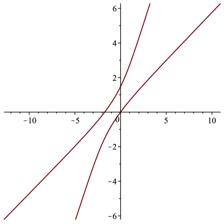
Figure 1: Scattering of two peakons with initial data (3.24) as a spacetime plot (time is the vertical axis).
To illustrate these results, it is instructive to consider a particular numerical example.
Upon choosing the initial data and parameters for (3.3) as
(3.24)
the values of the first integrals are
found to be
Then , and
so that lies between and , and also
where the latter quartic also has four real roots, namely
.
Substituting the roots of into (3.15) and setting at yields
, and similarly the integration constant in (3.18) can be fixed,
so that and are completely determined
parametrically in terms of . Figure 1 is a plot of their trajectories, with being the
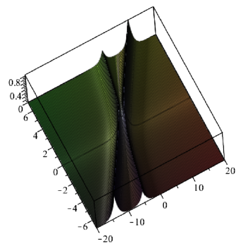
topmost curve. Figure 2 shows the same scattering process in the form
of a contour plot of viewed from above; the figure was made by joining
two different parametric plots, which were
required to deal with larger positive/negative
values separately.
The asymptotic amplitudes are
and
Then combining (3.22) and (3.23), we
find that the asymptotic positions of the two peakons are given by
where for the asymptotic velocities are
and for they are
Hence in this case the two peakons do not exactly exchange their asymptotic velocities and amplitudes, but only
approximately so.
Figure 2: Contour plot of in the box
, , .
4 Conclusions
We have considered the dynamics of peakon solutions in the non-integrable coupled system (1.12).
In the absence of a weak formulation appropriate for these solutions, they are interpreted as
distributional solutions in such a way that the peakons inherit the Hamiltonian properties of the PDE
system, so their dynamics is conservative. The two-peakon dynamics is Liouville integrable,
and we have explicitly integrated the equations of motion and described the interaction of the
peakons in the case when all the amplitudes are positive. The case where the amplitudes
have mixed sign (peakon-antipeakon interaction) is more subtle: in the Camassa-Holm case,
it involves a head-on collision, with overlapping peaks [4, 5]; while in this case,
if the peakons overlap () then the form of first integral , as in (3.8), implies that
at least
one of the amplitudes must diverge to infinity.
For three or more peakons, we do not expect that the dynamics of peakons is integrable.
Nevertheless, in the case where all the peakons have positive amplitudes, the qualitative
features of their interaction
should be similar to the two-peakon case. In particular, it is not hard to see that
the analogue of Lemma 4 holds for all : upon fixing ,
the fixed energy hypersurface
is a compact quadric in , so from the form of (2.9) there can
be no overlap between initially adjacent peaks; but then, from the
ordering (2.10), peaks that are initially non-adjacent cannot overlap without first passing through
their nearest neighbours, which cannot happen, holds, and the result follows.
Furthermore, it seems reasonable that the overall dynamics of three or more peakons should be
determined approximately by the local interaction between each pair of peaks, at least
when they are well separated from the rest.
It would be interesting to carry out numerical studies of the peakon ODEs (2.5) for , and
to perform a numerical integration of the full PDE system (1.12)
to see whether peakons emerge naturally from generic initial data, as is the case for the b-family
in the parameter range [15]. However, the PDE integration is likely to be at least as challenging as
for scalar peakon equations, which are already known to be difficult (for instance, see [7] and references).
Before embarking on such a study, it is worth noting that all
of the considerations in this paper admit a natural generalization to a
vector -family of PDEs, given by
with
being a -component vector of fields and a corresponding vector of parameters, and
where is a vector operator with components
So the original b-family (1.3) is just the case , while the
Popowicz system corresponds to with fields
and parameters .
Acknowledgements: LEB was supported by a studentship from SMSAS, University of Kent.
ANWH is supported by EPSRC fellowship EP/M004333/1, and is grateful to the
School of Mathematics & Statitsics, UNSW for hosting him as a Visiting
Professorial Fellow with additional funding from the Distinguished
Researcher Visitor Scheme. We also thank the reviewers for their comments.
References
[1] S.C. Anco, X. Chang and J. Szmigielski,
arXiv:1711.01429
[3] R. Beals, D.H. Sattinger and J. Szmigielski,
Adv. Math. 154 (2000) 229–257.
[4]
R. Camassa and D.D. Holm, Phys. Rev. Lett. 71 (1993) 1661–1664.
[5] R. Camassa, D.D. Holm and J.M. Hyman,
Adv. Appl. Mech. 31 (1994) 1–33.
[6] M. Chen, S.-Q. Liu and Y. Zhang,
Lett. Math. Phys. 75 (2006) 115.
[7] A. Chertock, J.-G. Liu and T. Pendleton,
SIAM J. Numer. Anal. 50 (2012) 1–21.
[8] A. Constantin and D. Lannes,
Arch. Ration. Mech. Anal. 192 (2009) 165–186.
[9] A. Degasperis and M. Procesi,
Asymptotic integrability, in Symmetry and Perturbation Theory, eds. Degasperis and G. Gaeta, River Edge, NJ: World Scientific (1999) 23–37.
[10] A. Degasperis, D.D. Holm and A.N.W. Hone, Theoret. Math. Phys. 133 (2002) 1461–1472.
[11] H.R. Dullin, G.A. Gottwald and D.D. Holm, Physica D 190 (2004) 1–14.
[12]
G. Falqui, J. Phys. A: Math. Gen. 39 (2006) 327–342.
[13] B. Fuchssteiner and A.S. Fokas,
Physica D 4
(1981) 47–66.
[14] D.D. Holm and A.N.W. Hone,
J. Nonlin. Math. Phys. 12 (2005) 380–394.
[15] D.D. Holm and M. Staley,
Phys. Lett. A 308 (2003) 437–444.
[16] A.N.W. Hone and M.V. Irle,
On the non-integrability of the Popowicz peakon system, in
Dynamical Systems and Differential Equations,
Proc. 7th AIMS International Conference,
Disc. Cont. Dyn. Sys. Supplement (2009) 359–366.
[17] A.N.W. Hone, H. Lundmark and J. Szmigielski,
Dyn. Partial Differ. Equ. 6 (2009) 253–289.
[18] M.V. Irle,
Solitons, peakons and Hamiltonian structure of particular partial differential equations,
MSc thesis, University of Kent, 2010.
[19] H. Lundmark and J. Szmigielski,
Int. Math. Res. Pap. IMRP 2005 (2005) 53–116.
[20] A.V. Mikhailov and V.S. Novikov, J. Phys. A: Math. Gen. 35 (2002) 4775–4790.
[21] Z. Popowicz, J. Phys. A: Math. Gen. 39 (2006) 13717–13726.