Encoding qubits into harmonic-oscillator modes via quantum walks in phase space

Abstract

We provide a theoretical framework for encoding arbitrary logical states of a quantum bit (qubit) into a continuous-variable quantum mode through quantum walks. Starting with a squeezed-vacuum state of the quantum mode, we show that quantum walks of the state in phase space can generate output states that are variants of codeword states originally put forward by Gottesman, Kitaev, and Preskill (GKP) [Phys. Rev. A 64, 012310 (2001)]. In particular, with a coin-toss transformation that projects the quantum coin onto the diagonal coin-state, we show that the resulting dissipative quantum walks can generate qubit encoding akin to the prototypical GKP encoding. We analyze the performance of these codewords for error corrections and find that even without optimization our codewords outperform the GKP ones by a narrow margin. Using the circuit representation, we provide a general architecture for the implementation of this encoding scheme and discuss its possible realization through circuit quantum-electrodynamics systems.

I Introduction

Computing based on quantum mechanical principles (i.e., quantum computing) requires exquisite control of quantum systems NC00 . Thanks to advancements in experimental techniques, tremendous progress has been made for achieving this goal during the past few years Ca17 . For large scale quantum computing, it is indispensable to have an architecture that enables efficient detection and correction of errors during the computing Li13 . Recently, there has been significant progress towards this direction in the field of continuous-variable (CV) measurement-based quantum computing, which seeks to achieve quantum computing by sequence of adaptive local measurements over highly entangled resource states in a state space with continuous spectrum Zh06 ; Me06 . In particular, Menicucci has shown that fault-tolerant quantum computing can be achieved in this scheme provided resource states with squeezing above $20.5$ dB are available Me14 . Recently, with the aid of topological codes, this squeezing threshold has been reduced to less than $10$ dB Fu17 ; Fu18 . Essential to these breakthroughs is a quantum error-correcting scheme due to Gottesman, Kitaev, and Preskill (GKP) GKP01 . In this approach, quantum information is encoded through a “hybrid” quantum bit (qubit) embedded in the (quantum mechanical) phase space of a quantum harmonic oscillator. Despite the importance of the GKP scheme, existing proposals for the experimental generation of GKP qubits remain to pose major challenges Tr02 ; Pi04 ; Pi06a ; Pi06b ; Va10 ; Br13 ; Te16 ; Mo17 ; We18 (see, however, the recent report in Ref. Fl19 ). In this paper we propose a new scheme for preparing GKP qubits through quantum walks (QWs) of an oscillator mode in phase space Ke03 ; Ma14 . As we will show, our encoding scheme indeed also provides a framework for experimentally accessing other general “grid states”, namely, codeword states with grid-like structures in phase space.

In the CV approach to quantum computing, quantum information are carried by quantum modes (aka “qumodes”) with the logical states encoded via eigenstates of the canonical coordinates of the field mode, which are usually likened to the position and momentum of a harmonic oscillator BP03 ; BrvL05 . Decoherence of the qumode then manifests as shift errors in these basis states. In order to correct such errors, GKP propose to invoke “hybrid” qubits that consist of superposition of uniformly spaced position eigenstates separated by $2\sqrt{\pi}$ GKP01

$$|0\rangle_{L} = \!\!\sum_{s=-\infty}^{\infty}\!\!|2s\sqrt{\pi}\,\rangle_{x}=\frac{1}{\sqrt{2}}\!\sum_{s=-\infty}^{\infty}\!\!|s\sqrt{\pi}\,\rangle_{p}\,,$$

$$|1\rangle_{L} = \!\!\sum_{s=-\infty}^{\infty}\!\!|(2s+1)\sqrt{\pi}\,\rangle_{x}=\frac{1}{\sqrt{2}}\!\sum_{s=-\infty}^{\infty}\!\!(-1)^{s}|s\sqrt{\pi}\,\rangle_{p},$$ (1)

where $|x\rangle_{x}$ and $|p\rangle_{p}$ are, respectively, position and momentum eigenstates. Thus the position-space wavefunctions for the codewords $|0\rangle_{L}$ and $|1\rangle_{L}$ comprise combs of delta functions located at, respectively, even and odd multiples of $\sqrt{\pi}$. In the presence of shift errors, it is then possible to correct sufficiently small errors in the encoded qubits through position and momentum measurements GKP01 . However, the GKP codeword states (1) require infinite squeezing, and hence infinite energy. In practice, therefore, one must approximate (1) with finitely squeezed states, such as uniformly spaced Gaussian spikes modulated by Gaussian envelopes GKP01

$${}_{x}\langle x|\tilde{l}\rangle_{L} \propto \sideset{}{{}^{\prime}}{\sum}_{n}\,e^{-\frac{n^{2}\pi\Delta_{p}^{2}}{2}}\,\exp\!\left[-\frac{(x-n\sqrt{\pi})^{2}}{2\Delta_{x}^{2}}\right],$$

$${}_{p}\langle p|\tilde{l}\rangle_{L} \propto \sum_{n}(-1)^{nl}\,e^{-\frac{\Delta_{x}^{2}\,p^{2}}{2}}\,\exp\!\left[-\frac{(p-n\sqrt{\pi})^{2}}{2\Delta_{p}^{2}}\right],$$ (2)

where $l=\{0,1\}$ are the logical bit values, $\sum_{n}^{\prime}$ in the position-space wavefunctions indicate summations over even/odd integers $n$ for $l=0/1$, and $\Delta_{x}$, $\Delta_{p}$ specify the widths of the Gaussians. It is our goal in the present paper to provide experimentally feasible schemes for engineering approximate GKP codewords such as (2) by implementing QWs in phase space for a qumode. In contrast to its classical counterpart, QW takes place in accordance with a quantum coin that admits superposition of orthogonal coin-states Ke03 ; Ma14 . Utilizing QWs of a qumode initially in a squeezed vacuum state, we will demonstrate that GKP-type codewords can be generated under appropriate “coin-toss rules”. As we will show, by changing the nature of the coin toss, one can attain GKP-type encodings with different characteristics. Our approach thus offers not only a promising pathway to the preparation of GKP qubits, but also opens up new dimensions to the GKP encoding.

In the following, we will start in Sec. II by first explaining how the features of QWs in phase space for a qumode can be exploited to encode a squeezed vacuum state into a GKP qubit. We will then illustrate with two instances: One involving generic unitary QWs, and the other dissipative, non-unitary QWs. Performance of our codewords for error correction will then be analyzed for the dissipative case. We will then discuss in Sec. III the implementation for our encoding scheme by first establishing a protocol using the circuit model and next touching on its possible experimental realizations through circuit quantum-electrodynamics systems. Finally, we conclude in Sec. IV with a summary and brief discussions for our findings. For presentational clarity, we relegate technical details and elaborate formulas to the Appendices.

II From quantum walk to the GKP encoding

Let us consider one-dimensional (1D) QW in phase space for a qumode with mode operator $\hat{a}=(\hat{x}+i\hat{p})/\sqrt{2}$, where $\hat{x}$ and $\hat{p}$ are, respectively, the “position” and “momentum” quadrature operators of the qumode. From the commutation relation $[\hat{a},\hat{a}^{\dagger}]=1$ for the mode operator, it follows that $[\hat{x},\hat{p}]=i$, which corresponds to setting $\hbar=1$ for us. For the QW, we will be concerned with position-squeezed states for the qumode, which will be denoted as $|q\rangle_{r}$. Here the subscript $r$ indicates the squeezing parameter, $q$ is the expectation value $\langle\hat{x}\rangle$ of the state in units of $\sqrt{2}$ times the QW step length $\xi_{d}$. Each step of the QW is conditioned on the configuration $|\epsilon\rangle$ of a two-state quantum coin with $\epsilon=\{R,L\}$ corresponding to rightward ($R$) and leftward ($L$) displacements by one single step length. More precisely, in terms of the phase-space displacement operator $\hat{D}(\xi)\equiv\exp\{\xi(\hat{a}^{\dagger}-\hat{a})\}$ for real $\xi$ and the squeezing operator $\hat{S}(r)\equiv\exp\{\frac{r}{2}(\hat{a}^{2}-\hat{a}^{\dagger 2})\}$ for real $r$, we will be considering squeezed coherent states

$$|q\rangle_{r}\equiv\hat{D}(q\,\xi_{d})\,\hat{S}(r)|{\rm vac.}\rangle$$ (3)

with $|{\rm vac.}\rangle$ the vacuum state of the qumode. Therefore, in the language of QW, the product state $|q\rangle_{r}|\epsilon\rangle$ indicates a walker at position $q\times\sqrt{2}\xi_{d}\equiv q\,x_{d}$ with a coin configuration $\epsilon$ (see footnote 1).

Let us suppose the QW has the coin-toss operator $\hat{\cal C}$. The corresponding “walk operator” would then read in the state space of (qumode)$\otimes$(coin)

$$\hat{W}=\hat{\cal T}(\xi_{d})\left(\hat{I}\otimes\hat{\cal C}\right)\,.$$ (4)

Here $\hat{I}$ is the qumode identity operator and $\hat{\cal T}$ is a translation operator whose action is conditioned on the coin configuration

$$\hat{\cal T}(\xi_{d})=\hat{D}(+\xi_{d})\otimes|R\rangle\langle R|+\hat{D}(-\xi_{d})\otimes|L\rangle\langle L|\,.$$ (5)

In order to prepare GKP qubits for the qumode, we shall consider 1D QW of a position-squeezed vacuum state along with a coin qubit in an arbitrary configuration

$$|\psi_{\rm in}\rangle=|0\rangle_{r}\left(\,\alpha|R\rangle+\beta|L\rangle\,\right)\,,$$ (6)

where $|\alpha|^{2}+|\beta|^{2}=1$. As we will demonstrate below, by means of 1D QW in phase space, one can transcribe the “logical state” imprinted in the coin configuration in (6) onto the qumode “coordinate” degrees of freedom $\{|q\rangle_{r}\}$. Since different choices for the coin-toss transformation $\hat{\cal C}$ can lead to rather distinct walk patterns in the QW Ke03 ; Ma14 , it can be anticipated that different encodings can be achieved through different coin-toss transformations. In the following, we will consider first the case of a “Hadamard coin-toss”, which induces unitary evolution of the input state (6). As we shall find out, the consequent codewords will be quite different from the approximate GKP codewords in (2). We will then turn to another coin-toss transformation, which will engender codeword states that are similar to the “standard” ones in (2).

II.1 Generic (unitary) quantum-walk encoding

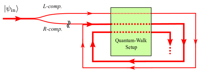
Figure 1: Conceptual layout for our QW-encoding scheme, where each thin line represents the respective component of the input state $|\psi_{\rm in}\rangle$ [see Eq. (6)] as indicated, while heavy lines stand for the full state. Each passing (dashed line) of the state through the QW-setup implements for the qumode one single step of QW in phase space. Before entering the QW-setup, the input state $|\psi_{\rm in}\rangle$ is split into its $R$ and $L$-components, with the $R$-component subsequently delayed behind the $L$-component. After the $L$-component has completed one single step of QW while none for the $R$-component, the two are combined for the ensuing QWs. The encoded state is generated after the combined state has completed the designated steps of QW.

For a walker that localizes initially at the origin, after even (odd) steps of QW the wavefunction of the walker would become coherent superposition of localized states over even (odd) multiples of the step length. In view of the structure of the ideal GKP codewords (1), it is clear that one can exploit this feature of QWs to prepare GKP qubits. The conceptual plan for our encoding scheme is outlined in Fig. 1. In order to simplify our theoretical formulation, let us suppose for now that when implementing the QW, we are able to separate and combine the components, e.g. $|0\rangle_{r}|R\rangle$ and $|0\rangle_{r}|L\rangle$ (which, for brevity, will be referred to as the $R$ and $L$-components, respectively) of the input state (6) in the way shown in Fig. 1. As we shall find out, this serves only as a convenience to help present our theoretical ideas in a clear way, but won’t be a necessity in physical implementations for the scheme, which we shall discuss in Sec. III.

In our encoding scheme, as shown in Fig. 1, prior to the QW we separate the $R$ and the $L$-components of the input state (6) to produce a time gap between them. In the scenario of Fig. 1, we delay the $R$-component so that when it begins its QW, the $L$-component would have completed exactly one step of QW. The two components are then combined for all subsequent QWs. Since the $R$-component always lags behind the $L$-component by one single step, in the course of the QW coherent superposition of localized spikes at sites of opposite parities are generated progressively for the two components of the input state. Therefore, a GKP-type encoding can be furnished after the state has completed the desired number of steps of QW.

As an illustration, let us consider an encoding with the following coin-toss transformation in the coin basis $\{|R\rangle,|L\rangle\}$

$$\hat{\cal C}_{H}=\frac{1}{\sqrt{2}}\left(\begin{array}[]{cc}1&1\\ 1&-1\\ \end{array}\right)\,,$$ (9)

which corresponds to a Hadamard coin-toss for the QW Ma14 . Suppose the initial state (6) undergoes the encoding process of Fig. 1, so that its $R$ and $L$-components would complete, respectively, $N$ and $(N+1)$ steps of QW upon output. It then leads to the state

$$|\psi_{\rm out}\rangle=\alpha|\psi_{N}^{(R)}\rangle+\beta|\psi_{N+1}^{(L)}\rangle\,,$$ (10)

where $|\psi_{N}^{(\epsilon)}\rangle$ with $\epsilon=\{R,L\}$ are the resulting states for $|0\rangle_{r}|\epsilon\rangle$ after $N$ steps of QW. One can find analytically that Am01

$$|\psi_{N}^{(\epsilon)}\rangle=\sideset{}{{}^{\prime}}{\sum}_{n=-N}^{N}\,\,|n\rangle_{r}\left(u_{N}^{(\epsilon)}(n)|R\rangle+v_{N}^{(\epsilon)}(n)|L\rangle\right)\,,$$ (11)

where $\sum_{n}^{\prime}$ indicates summation over every other integers, that is, $n=\{-N$, $-(N-2)$, $\dots$, $(N-2)$, $N\}$. To avoid distractions, we supply explicit expressions for the amplitudes $u_{N}^{(\epsilon)}(n)$ and $v_{N}^{(\epsilon)}(n)$ in Appendix A.1. From (11), it is then clear that when $N$ is, for instance, even $|\psi_{N}^{(R)}\rangle$ in (10) would cover only even sites, while $|\psi_{N+1}^{(L)}\rangle$ only odd sites. By defining the encoded logical basis states here

$$|0\rangle_{\rm QW}\equiv|\psi_{N}^{(R)}\rangle\quad{\rm and}\quad|1\rangle_{\rm QW}\equiv|\psi_{N+1}^{(L)}\rangle\,,$$ (12)

we then have from (10) the encoded state for the input state (6)

$$|\psi_{\rm encd}\rangle=\alpha|0\rangle_{\rm QW}+\beta|1\rangle_{\rm QW}\,.$$ (13)

Our scheme thus furnishes a GKP-type encoding for an arbitrary input state.

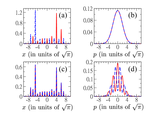
Figure 2: Probability densities in position space and momentum space for generic QW-codewords with $N=8$ at a squeezing with $e^{-r}=0.2$ ($\sim$13.98 dB). Panels (a) and (b) illustrate the results for $|0\rangle_{\rm QW}$ (solid curves) and $|1\rangle_{\rm QW}$ (dashed curves), while panels (c) and (d) show those for $|+\rangle_{\rm QW}\equiv(|0\rangle_{\rm QW}+|1\rangle_{\rm QW})/\sqrt{2}$ (solid curves) and $|-\rangle_{\rm QW}\equiv(|0\rangle_{\rm QW}-|1\rangle_{\rm QW})/\sqrt{2}$ (dashed curves).

To find the position-space and the momentum-space wavefunctions for the codewords $|0\rangle_{\rm QW}$ and $|1\rangle_{\rm QW}$, we note that from (3) one can obtain the wavefunctions for the squeezed coherent states $|n\rangle_{r}$

$${}_{x}\langle x|n\rangle_{r} = \frac{e^{+\frac{r}{2}}}{\pi^{\frac{1}{4}}}\exp\!\left[\frac{-(x-n\,x_{d})^{2}}{2\,e^{-2r}}\right]\,,$$

$${}_{p}\langle p|n\rangle_{r} = \frac{e^{-\frac{r}{2}}}{\pi^{\frac{1}{4}}}\exp\!\left[+i\,n\,x_{d}\,p-\frac{p^{2}}{2\,e^{+2r}}\right]\,,$$ (14)

where $x_{d}\equiv\sqrt{2}\xi_{d}$, as before (see footnote 1). Making use of (14), one can obtain the wavefunctions for the codeword states $|0\rangle_{\rm QW}=|\psi_{N}^{(R)}\rangle$ and $|1\rangle_{\rm QW}=|\psi_{N+1}^{(L)}\rangle$ using (11) and the expressions for the amplitudes $u_{N}^{(\epsilon)}$, $v_{N}^{(\epsilon)}$, and etc. in Appendix A.1. Setting $x_{d}=\sqrt{\pi}$ for the QW, we show in Fig. 2 the probability densities in position and momentum spaces for the QW-codewords $|0\rangle_{\rm QW}$ and $|1\rangle_{\rm QW}$, together with the conjugate states $|+\rangle_{\rm QW}\equiv(|0\rangle_{\rm QW}+|1\rangle_{\rm QW})/\sqrt{2}$ and $|-\rangle_{\rm QW}\equiv(|0\rangle_{\rm QW}-|1\rangle_{\rm QW})/\sqrt{2}$ for the case of $N=8$ at a squeezing with $e^{-r}=0.2$ (corresponding to $\sim$13.98 dB squeezing).

From Fig. 2, we see that, despite the unusual envelopes, the probability densities of the QW-codewords exhibit features characteristic of approximate GKP codewords that are essential for correcting shift errors Pi04 . In particular, the position distributions of the codewords $|0\rangle_{\rm QW}$ and $|1\rangle_{\rm QW}$ consist of Gaussian spikes at, respectively, even and odd multiples of $\sqrt{\pi}$, while the momentum distributions of the codewords $|+\rangle_{\rm QW}$ and $|-\rangle_{\rm QW}$ manifest peaks at, respectively, even and odd multiples of $\sqrt{\pi}$. Therefore, in principle, the QW-codewords here can be adopted to correct shift errors in accordance with the GKP scheme, despite the issues with their performance and probably also efficiencies Me14 . The key drawbacks of the QW-codewords (12) reside in their momentum distributions, such as the featureless Gaussians in Fig. 2(b) for $|0\rangle_{\rm QW}$ and $|1\rangle_{\rm QW}$, and the broad peaks in Fig. 2(d) for $|+\rangle_{\rm QW}$ and $|-\rangle_{\rm QW}$, which would render the correction for $p$-errors ineffective. We find numerically that these features are independent of the QW steps $N$, likely due to unitarity of the QW here. Since different coin-toss transformations for QW can lead to very different walk patterns Ke03 ; Ma14 , one possible remedy for the present dilemma is to replace the coin-toss operation (9) with a new one. Alternatively, since the difficulty with the codewords $|0\rangle_{\rm QW}$ and $|1\rangle_{\rm QW}$ lies in the lack of (coin-state independent) structures in their momentum distributions, one can attempt to implement periodic structures in both position and momentum directions through two-dimensional QWs Ma14 . As our point here is to demonstrate the feasibility of the proposed QW-scheme for generating GKP-type encodings in a generic setting, we shall not pursue these issues further.

In addition to the “unconventional” profiles in the probability densities of the QW-codewords in Fig. 2, it should be noted that here the codewords $|0\rangle_{\rm QW}$ and $|1\rangle_{\rm QW}$ are entangled states between the qumode and the ancillary coin-qubit [see (11)]. This is in stark contrast to codewords from the original GKP-scheme, where the encoding resides entirely in the qumode. To disentangle the qumode from the coin qubit in the QW-codewords, one can choose to project them onto any given coin state, such as the symmetric “diagonal” coin-state $|D\rangle\equiv(|R\rangle+|L\rangle)/\sqrt{2}$. However, we find this would lead to states that are plagued by fast oscillations of intervals below $\sqrt{\pi}$ in their momentum-space distributions, which are unfavorable for correcting $p$-errors. Therefore, here we choose to retain the form (11) for the QW-codewords with its full generality. At this point, it is then natural to ask whether our scheme is capable of producing QW-codewords akin to the “standard” GKP ones as in (2) or not. As we will now show, this is indeed possible if appropriate coin-toss transformation is used.

II.2 Dissipative (non-unitary) quantum-walk encoding

In order to generate codewords similar to (2), it necessitates implementing QWs with Gaussian probability distributions in our scheme. Intuitively, one might expect decoherence of the state must be incorporated, so that the QW would become classical and yield the desired probability distributions Ke07 . However, this would inevitably lead to mixed states, which are unfavorable for our purposes here, as the codeword states must be pure states. To find the way out, we note that the nonclassical nature of the QW arises from the interference between the coin-toss outcomes for the $R$ and the $L$-components. Therefore, if we project the state vector at each step of the QW, so that the two coin-state components won’t interfere, it would then be possible to generate coherent superposition of “classically” distributed Gaussian spikes. In other words, by “resetting” the coin state of the walker to a symmetric combination of the $|R\rangle$ and the $|L\rangle$ states in each step of the QW, one can then generate the desired walk pattern here. It thus follows that one should replace the coin-toss transformation (9) with the projection operator for the diagonal coin-state $|D\rangle=(|R\rangle+|L\rangle)/\sqrt{2}$, i.e.,

$$\hat{\cal C}_{D}=|D\rangle\langle D|=\frac{1}{2}\left(\begin{array}[]{cc}1&1\\ 1&1\\ \end{array}\right)\,.$$ (17)

With this change, as we shall show below, we are then able to achieve the targeted codeword states. Since the projection operator can reduce the total probability of the state it acts on, the QW here becomes nonunitary, and we shall refer to it as the “dissipative” QW.

For the QW-encoding modified with the new coin-toss operation (17), the calculation for the corresponding encoded states proceeds in exactly the same manner as before. After the $R$-component and the $L$-component of the input state (6) have completed, respectively, $N$ and $(N+1)$ steps of QW, one can find an output state with the same structure as Eqs. (10) and (11), but now with different explicit forms for the amplitudes $u_{N}^{(\epsilon)}(n)$ and $v_{N}^{(\epsilon)}(n)$ (see Appendix A.2). At this point, it is tempting to conclude immediately that the encoding can then be done in exactly the same way as in (12). This is, however, incorrect because we now have nonunitary, dissipative QWs and thus must take extra care for the normalization of the state vectors. Moreover, in order that the codeword states would resemble better the approximate GKP codewords (2), we find it advantageous to project the final state of the QW onto the diagonal coin-state $|D\rangle$, which also serves to disentangle the qumode from the coin qubit here. For the initial state $|0\rangle_{r}|\epsilon\rangle$ the resulting unnormalized state vector after $N$ steps of dissipative QW (including the action of the $|D\rangle$-projector upon output) takes the form

$$|\psi_{N}\rangle=\sideset{}{{}^{\prime}}{\sum}_{n=-N}^{N}\!w_{N}(n)\,\,|n\rangle_{r}|D\rangle\,,$$ (18)

where

$$w_{N}(n)=\frac{1}{2^{N+\frac{1}{2}}}\left(\begin{array}[]{c}N\\ \frac{N+n}{2}\\ \end{array}\right)\,.$$ (21)

Notice that here the qumode and the coin qubit are fully disentangled. Also, since the $R$ and the $L$-components are now symmetrical, we have dropped the superscript $\epsilon$ for the initial coin configurations in (18) and (21) [cf. Eq. (11) for the unitary case]. In terms of the normalized state vectors for (18)

$$|\phi_{N}\rangle\equiv Z_{N}^{-1/2}|\psi_{N}\rangle$$ (22)

with $Z_{N}\equiv\langle\psi_{N}|\psi_{N}\rangle$, we find the output state for the dissipative QW

$$|\psi_{\rm out}\rangle = \alpha\,\sqrt{Z_{N}}\,\,|\phi_{N}\rangle+\beta\,\sqrt{Z_{N+1}}\,\,|\phi_{N+1}\rangle$$ (23)

$$\propto \alpha^{\prime}|\phi_{N}\rangle+\beta^{\prime}|\phi_{N+1}\rangle\,,$$

where we have denoted in the second line $\alpha^{\prime}\equiv\alpha/\sqrt{|\alpha|^{2}+\gamma^{2}|\beta|^{2}}$ and $\beta^{\prime}\equiv\gamma\beta/\sqrt{|\alpha|^{2}+\gamma^{2}|\beta|^{2}}$ with $\gamma\equiv\sqrt{Z_{N+1}/Z_{N}}$. Therefore, identifying

$$|0\rangle_{\rm dQW}\equiv|\phi_{N}\rangle\quad{\rm and}\quad|1\rangle_{\rm dQW}\equiv|\phi_{N+1}\rangle\,,$$ (24)

we arrive at the following encoding for the input state (6)

$$|\psi_{\rm encd}\rangle={\cal N}\,(\,\alpha^{\prime}|0\rangle_{\rm dQW}+\beta^{\prime}|1\rangle_{\rm dQW}\,)$$ (25)

with ${\cal N}\equiv\sqrt{|\alpha|^{2}Z_{N}+|\beta|^{2}Z_{N+1}}$. Notice that the coefficients $\alpha$, $\beta$ in the original state (6) have been modified in the final encoding (25) due to the dissipative nature of the QW. Therefore, when applying this encoding scheme, one must prepare the input state properly, so that the desired encoded states can be obtained at the output.

To find the wavefunctions of the codewords here, one can again use (14) in (24) [together with Eqs. (18)–(22)]. For the momentum-space wavefunction, the summation over the site index $n$ can be done analytically. We find

$${}_{p}\langle p|\phi_{N}\rangle=\left(\frac{e^{-r}}{2\sqrt{\pi}Z_{N}}\right)^{\!\!\frac{1}{2}}\!\!\exp\!\!\left[-\frac{p^{2}}{2\,e^{+2r}}\right]\!\cos^{N}\!(x_{d}\,p)|D\rangle\!.$$ (26)

For the position-space wavefunction, it is of particular interest to examine its large $N$ limit, for which the binomial distribution would tend to a Gaussian. Applying Stirling’s formula, we find for large $N$

$${}_{x}\langle x|\phi_{N}\rangle\approx\left(\frac{2e^{+r}}{\pi\sqrt{N}}\right)^{\!\!\frac{1}{2}}\!\!\!\sideset{}{{}^{\prime}}{\sum}_{n=-N}^{N}\!e^{-\frac{n^{2}}{2N}}\,\exp\!\!\left[-\frac{(x-n\,x_{d})^{2}}{2\,e^{-2r}}\right]|D\rangle\,.$$

(27)

For the normalization in (27), we have taken the squeezed coherent states $\{|n\rangle_{r}\}$ here to be approximately orthogonal, so that $Z_{N}$ in (22) can be approximated as

$$Z_{N}\approx\frac{1}{2^{2N+1}}\left(\begin{array}[]{c}2N\\ N\\ \end{array}\right)\approx\frac{1}{2\sqrt{\pi N}}\,.$$ (30)

Taking $x_{d}=\sqrt{\pi}$ in (27) and comparing the expression with the approximate GKP codewords (2), we see that in the large $N$ limit the dissipative QW (or dQW, for short) codewords (24) correspond to approximate GKP codewords with width $\Delta_{x}\approx e^{-r}$ and $\Delta_{p}\approx 1/\sqrt{\pi N}$. Therefore, for shift errors symmetric in the position and the momentum quadratures, following GKP GKP01 , the choice for encodings with $\Delta_{x}=\Delta_{p}$ becomes here $e^{+r}=\sqrt{N\pi}$. As an illustration, we plot in Fig. 3 the wavefunctions for the dQW-codewords for the case with $N=8$ and $e^{-r}=1/\sqrt{8\pi}\sim 0.199$ (corresponding to $\sim 14.00$ dB squeezing), which carry the hallmarks of approximate GKP codewords (2).

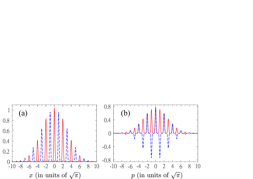
Figure 3: (a) Position and (b) momentum wavefunctions for the dissipative QW-codewords $|0\rangle_{\rm dQW}$ (solid curves) and $|1\rangle_{\rm dQW}$ (dashed curves) with $N=8$ at a squeezing with $e^{-r}=1/\sqrt{8\pi}\sim 0.199$ ($\sim 14.00$ dB squeezing).

In order to evaluate the performance of the dQW-codewords (24), we consider the error-correcting scheme of Ref. Gl06 and find the probability $P_{\mbox{\scriptsize no error}}$ for repeated error corrections using the dQW-codewords without incurring Pauli errors (see Appendix B for details). For this calculation, we consider $N$-step dissipative QW-encoding with width $e^{-r}=1/\sqrt{N\pi}\equiv\Delta$. The results are shown in Fig. 4, where we also plot the results for the approximate GKP codewords (2) with $\Delta_{x}=\Delta_{p}=\Delta$ for comparison. It is encouraging to find that the dQW-codewords in fact outperform their GKP counterparts for all $\Delta$ by a small margin. In particular, for the $N=8$ dQW-codewords we get $P_{\mbox{\scriptsize no error}}\simeq 0.936$ [vs. $\simeq 0.929$ for the GKP case] at the squeezing $\sim 14.00$ dB, which is within current experimental capabilities Va16 . Although for dQW-codewords with $N=10$ one can even attain $P_{\mbox{\scriptsize no error}}\simeq 0.966$ at a squeezing $\sim 14.97$ dB, which lies barely below the 15 dB squeezing achieved in Ref. Va16 , implementing 10 and 11 steps of QW are even more challenging experimentally.

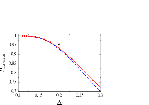
Figure 4: The probability for repeated error corrections without Pauli errors using dissipative QW-codeword $|0\rangle_{\rm dQW}$ (dots) with $\Delta=e^{-r}=1/\sqrt{N\pi}$, where the solid line serves as guide to the eyes. For comparison, we also plot the results for the approximate GKP codeword $|\tilde{0}\rangle_{L}$ (dashed line) with $\Delta_{x}=\Delta_{p}=\Delta$ in (2). The arrow indicates the point for $N=8$ and $\Delta=1/\sqrt{8\pi}\sim 0.199$ (corresponding to $\sim 14.0$ dB squeezing) in the dissipative QW-codeword.

III Implementations

We shall now look into the physical implementations for our QW-encoding scheme. To begin with, let us take the coin states $|R\rangle$ and $|L\rangle$, respectively, the logical zero and the logical one states of a control qubit for a controlled-displacement gate, and write the walk operator $\hat{W}$ of (4) as

$$\hat{W}=\left[\hat{I}\otimes|R\rangle\langle R|+\hat{D}(-2\xi_{d})\otimes|L\rangle\langle L|\right]\,\left(\hat{D}(+\xi_{d})\otimes\hat{\cal C}\right)\,.$$ (31)

It then follows that the walk operator $\hat{W}$ can be implemented through the quantum circuit depicted in Fig. 5(a). To prepare logical basis states in the QW-scheme [i.e., (12) or (24)], one can thus supply the states $|0\rangle_{r}|R\rangle$ and $|0\rangle_{r}|L\rangle$ to the circuit separately and cycle for the corresponding numbers of rounds for the QW. It is to be noted that for the dissipative QW-encoding of Sec. II.2, an additional projection operator $|D\rangle\langle D|$ over the coin degree of freedom has to be applied at the output of the final round of QW [see above Eq. (18)], which is not included in the circuit of Fig. 5(a). To encode qubits with arbitrary logic, however, it requires additional efforts, as one has to delay either the $R$ or the $L$-component of the general input state (6) for the encoding.

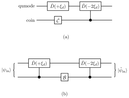
Figure 5: Quantum circuits for (a) implementing one single step of QW and (b) preparing the properly delayed state $|\tilde{\psi}_{\rm in}\rangle$ from the input state $|\psi_{\rm in}\rangle$. Here $\hat{D}$ is the phase-space displacement operator, $\hat{\cal C}$ the coin-toss operator for the QW, and $\hat{\cal B}$ the “biased” coin-toss operator for state preparation (see text).

As previously, let us delay the $R$-component of the input state one step behind its $L$-component for the QW. It then suffices if we are able to prepare from the input state $|\psi_{\rm in}\rangle$ the corresponding “delayed state” $|\tilde{\psi}_{\rm in}\rangle$, which has the $L$-component already taken one step of QW, while none for the $R$-component, that is,

$$|\tilde{\psi}_{\rm in}\rangle = \alpha|0\rangle_{r}|R\rangle+\beta\,\hat{W}\,|0\rangle_{r}|L\rangle\,.$$ (32)

For instance, in the case of the unitary QW-encoding with a Hadamard coin (9) discussed in Sec. II.1, the desired delayed state would then be

$$|\tilde{\psi}_{\rm in}\rangle_{\rm QW}=\alpha|0\rangle_{r}|R\rangle+\frac{\beta}{\sqrt{2}}\left(|+1\rangle_{r}|R\rangle-|-1\rangle_{r}|L\rangle\right)\,.$$ (33)

As shown in Appendix C, this state can be produced from the input state $|\psi_{\rm in}\rangle$ making use of the circuit illustrated in Fig. 5(b), which has two controlled-displacement operators separated by a “biased” coin-toss operator $\hat{\cal B}=\hat{\cal B}_{H}$ given by

$$\hat{\cal B}_{H}=\left(\begin{array}[]{cc}1&0\\ \frac{1}{\sqrt{2}}&\frac{-1}{\sqrt{2}}\\ \end{array}\right)\,.$$ (36)

Comparing (36) with (9), we see that $\hat{\cal B}_{H}$ does not flip the $R$-component of the quantum coin, while tosses its $L$-component in the way of the Hadamard coin $\hat{\cal C}_{H}$ (thus, a “biased” coin-toss). It is therefore not surprising that the delayed state can be duly prepared this way.

Similarly, for the dissipative QW-encoding of Sec. II.2 the necessary delayed state can be obtained using (32) and the corresponding walk operator. The result reads

$$|\tilde{\psi}_{\rm in}\rangle_{\rm dQW}=\alpha|0\rangle_{r}|R\rangle+\frac{\beta}{2}\left(|+1\rangle_{r}|R\rangle+|-1\rangle_{r}|L\rangle\right)\,.$$ (37)

Again, this state can be prepared through the circuit of Fig. 5(b) with the following biased coin-toss

$$\hat{\cal B}_{D}=\left(\begin{array}[]{cc}1&0\\ \frac{1}{2}&\frac{1}{2}\\ \end{array}\right)\,.$$ (40)

Once the delayed state is available, for both encoded states (13) and (25) discussed in Sec. II, the remaining $N$ steps of QW can then be implemented by sending the respective $|\tilde{\psi}_{\rm in}\rangle$ into the circuit of Fig. 5(a) and cycling for $N$ rounds. As before, in the dissipative case an additional projector $|D\rangle\langle D|$ over the coin qubit must be incorporated into the circuit of Fig. 5(a) at the output of the final round.

With the architecture for implementing QW-encodings in place, it is of interest to examine how it can be realized in practice. One possible route that may be accessible to current technologies is offered by extending the circuit quantum-electrodynamics (cQED) setup for implementing the cat code Co99 ; Le13 ; Vl13 ; Of16 . To realize our encoding scheme, we see from Fig. 5 that it calls for implementing conditional and unconditional qumode phase-space displacements, along with coin operations with biased ($\hat{\cal B}$) and fair ($\hat{\cal C}$) coin-toss. As we shall explain below, these gate operations can be implemented efficiently using cQED systems, as demonstrated previously in the cat code and other experiments.

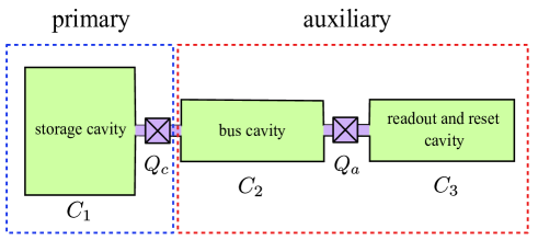
Figure 6: Schematics of the proposed cQED setup for implementing the QW-encoding, which is separated into the primary and the auxiliary parts. The primary part consists of the main components for the encoding, where a storage cavity ($C_{1}$) stores the codeword state and a transmon qubit ($Q_{c}$) acts as the quantum coin for the QW. In order to implement coin-toss operations, the auxiliary part contains an ancilla qubit ($Q_{a}$) that is coupled to the coin qubit ($Q_{c}$) through a bus cavity ($C_{2}$). Also in the auxiliary part is another cavity ($C_{3}$) attached to the ancilla qubit ($Q_{a}$), which serves to read out and reset the ancilla states at different stages of the encoding.

Let us consider the setup depicted schematically in Fig. 6, which consists of three waveguide cavity resonators $C_{1}\sim C_{3}$ intercepted with two superconducting transmon qubits $Q_{c}$ and $Q_{a}$. For clarity, we have divided the setup into two parts: the primary and the auxiliary parts. Here the primary part consists of cavity $C_{1}$ for storing the codeword state during the encoding process, and qubit $Q_{c}$ playing the role of the quantum coin for the QW. The auxiliary part of the setup here serves to furnish the coin-toss transformations required for the encoding, including the biased one ($\hat{\cal B}$) for state preparation and the fair one ($\hat{\cal C}$) for each step of the QW. It is comprised of an ancillary qubit $Q_{a}$ connected to a bus cavity $C_{2}$ for mediating coupling with the coin qubit $Q_{c}$, together with cavity $C_{3}$ for measuring and resetting the ancilla state during the QW.

To understand how the setup works, let us recall that generically the interaction between a transmon qubit and a cavity mode is well approximated by the Jaynes-Cummings Hamiltonian Bl04 ; Gi14 ; We17

$$\frac{\hat{H}_{\rm JC}}{\hbar}=-\frac{\omega_{q}}{2}\hat{Z}+\omega_{r}\hat{a}^{\dagger}\hat{a}+g\left(\,\hat{a}^{\dagger}\otimes\,|0\rangle\langle 1|+\hat{a}\otimes|1\rangle\langle 0|\,\right)\,.$$ (41)

Here $\hat{Z}\equiv\left(|0\rangle\langle 0|-|1\rangle\langle 1|\right)$ is the Pauli-$Z$ operator for the qubit with $|0\rangle$ and $|1\rangle$, respectively, the lower and upper qubit levels that are separated by frequency $\omega_{q}$ apart. $\hat{a}$ is the mode operator for the cavity mode with frequency $\omega_{r}$, and $g$ characterizes the qubit-cavity interaction strength. In the regime of large detuning, $\delta\equiv(\omega_{q}-\omega_{r})\gg g$ (the strong dispersive regime), one can derive perturbatively an effective Hamiltonian from (41) Gi14 ; Sc01

$$\frac{\hat{H}}{\hbar}=-\frac{(\omega_{q}+\chi)}{2}\hat{Z}+\omega_{r}\hat{a}^{\dagger}\hat{a}-\chi\,\hat{a}^{\dagger}\hat{a}\otimes\hat{Z}\,,$$ (42)

where $\chi\equiv g^{2}/\delta$ is the qubit frequency shift (the “Lamb shift”) due to the cavity coupling. It is the effective qubit-cavity coupling $\hat{V}_{I}\equiv-\chi\,\hat{a}^{\dagger}\hat{a}\otimes\hat{Z}$ in (42) that enables efficient control and manipulations of qubit and cavity states in this strong dispersive regime Bl04 ; Ha06 . In particular, time evolution due to the coupling $\hat{V}_{I}$ induces a qubit-state dependent phase-space rotation of the cavity mode, which yields for a time duration $t$

$$e^{-i\chi t\,\hat{a}^{\dagger}\hat{a}\otimes\hat{Z}}=e^{-i\chi t\,\hat{a}^{\dagger}\hat{a}}\otimes|0\rangle\langle 0|+e^{+i\chi t\,\hat{a}^{\dagger}\hat{a}}\otimes|1\rangle\langle 1|\,.$$ (43)

As detailed in Appendix D.1, the evolution operator (43) can help implement the conditional cavity displacement operation that is key to the QW-encoding (see Fig. 5). At the same time, since $\hat{V}_{I}$ commutes with both the qubit and the cavity Hamiltonians, it allows quantum non-demolition measurement of the qubit state or the cavity state Ha06 . In our case, this is utilized in the setup of Fig. 6 to read out the ancilla ($Q_{a}$) state through its coupling with cavity $C_{3}$.

Extending the consideration above to the case of two transmon qubits jointly coupled to a cavity bus resonator, the off-resonant coupling can then mediate an indirect interaction between the pair of qubits Bl04 ; Ma07 . If higher qubit excitations are taken into account, they can be exploited to furnish two-qubit gates, such as the conditional phase gate Di09 that is helpful for implementing the coin-toss transformations for the QW-encoding–the task of the auxiliary components in Fig. 6. For example, to effect the biased coin-toss operation $\hat{\cal B}$ on the coin qubit, it can be done by realizing a suitable positive operator-valued measure (POVM) for this operation. To this end, it is necessary to introduce an ancilla qubit coupled to the coin qubit and enact two-qubit controlled gates along with single-qubit gates. Subsequent ancilla measurement would then signal success/failure of the gate operation. In the auxiliary part of the setup in Fig. 6, the bus cavity ($C_{2}$) serves to mediate the desired two-qubit coupling between the coin qubit and the ancilla qubit, and the readout cavity ($C_{3}$) provides the means for detecting the ancilla state. It should be noted that the ancilla qubit must be reset to its initial configuration after each run of the coin-toss, which can be done through feedback controlled pulses via cavity $C_{3}$ Of16 . In Appendix D, we demonstrate the scheme for realizing the coin-toss operations in the dissipative QW-encoding, where both the biased and the fair coin-toss operations will be considered.

It should be noted that our discussions above for the cQED implementation have entirely left out nonlinearity effects inherent in such systems. In a more quantitative analysis, these must be taken into account properly. Also, we point out that our implementations for the coin-toss operations for the dissipative QW-encoding demonstrated in Appendix D are non-deterministic. With increasing number of QW steps $N$, the overall success rate for the QW-encoding drops exponentially $\sim 1/2^{N}$. This can also be anticipated from the form of the (fair) coin-toss operator $\hat{\cal C}_{D}$ given by (17), which projects the state progressively in the course of the QW, reflecting the “dissipative” nature of the QW. Thus, in practice, the dissipative QW-encoding would work only for small numbers of $N$. In spite of this, since the recently achieved first experimental realization for the GKP codewords Fl19 corresponds to $N\sim 2$ in our case, we think the dissipative QW-encoding should be still of experimental interest. Moreover, we use the dissipative QW-encoding to demonstrate how the QW-encoding scheme can be adapted to generate approximate GKP codewords akin to the “standard” forms (2). Ultimately, we wish to devise a robust unitary QW-encoding (or a unitary encoding process for general QW-codewords) which would alleviate the loss problem. Nevertheless, it should be noted that the preparation for the “delayed states” (32) in our QW-encoding is always nonunitary. Even for a unitary (fair) coin, this state preparation has a weak nonunitarity due to the finite overlap between the squeezed coherent states $|0\rangle_{r}$ and $|+1\rangle_{r}$. In practice, however, this nonunitarity would be rather small and for QW-encoding with a unitary coin one can safely take it to be unitary to good approximations.

Finally, we remark that in preparing GKP-type codeword states from the squeezed vacuum the process must be non-Gaussian GKP01 . From our discussions for the cQED implementation of the QW-encoding, we see that by coupling the qumode to a quantum coin, one can enact effective non-Gaussian evolution of the qumode, which underlies the codewords’ robustness against shift errors. In order to improve the robustness of the codewords, as exemplified by the dissipative QW-encoding, it seems nonunitary coin operation can be advantageous for enhancing nonlinearity in the qumode dynamics. There thus seems to be a trade-off between unitarity and codeword robustness in the QW-encoding: Unitarity is favored for preserving codeword intensity, but not for promoting its robustness. To achieve robust GKP-type codeword states with optimum intensities, therefore, it is necessary to optimize through the coin-toss operation $\hat{\cal C}$ for the QW-encoding.

IV Conclusion and Discussions

In summary, we have shown that by implementing QWs in phase space for a qumode, it is possible to furnish GKP-type encodings for quantum error-corrections in CV quantum computing. In addition to demonstrating an encoding through generic unitary QWs that produces codewords with “unconventional” profiles, we show further that an encoding via dissipative, nonunitary QWs can generate codeword states similar to the standard GKP ones. We examine the performance of the dissipative QW-codewords for error corrections and find that they do better than the standard GKP codewords by a small amount. In view of this result, it is promising that with optimized coin-toss transformations, one may find QW-codewords that perform even better. Although platforms for implementing QWs may not be easily tailored to the needs of universal quantum computing Ma14 , we have proposed an architecture for bridging this gap through cQED systems.

Throughout this work we have based our encoding scheme on the discrete-time quantum walk (DTQW). It is pertinent to enquire whether one could, instead, resort to continuous-time quantum walk (CTQW) for the task or not. Despite the fact that it is possible to map between DTQW and CTQW in 1D space St06 , due to the lack of the coin degree of freedom in CTQW, we find DTQW provides a framework that connects more directly to the encoding that we wish to implement. Nevertheless, it remains an interesting open question as to whether CTQW can offer additional advantages to the QW-encoding or not.

Although we have focused primarily on engineering the GKP codeword states, our work indeed uncovers a new avenue to accessing general GKP-type “grid states”. For instance, as pointed out earlier, extending our encoding scheme to the case of two-dimensional QWs can be useful for rectifying the undesirable momentum distributions of the codewords in Fig. 2. At the same time, this may also help enhance the versatility of the QW-encoding scheme. In view of the multitude of walk patterns available for QWs Ke03 ; Ma14 , the QW-encoding scheme proposed in this work thus opens up a new dimension for the GKP encoding that is yet to be explored. In particular, it may offer a unified framework for experimentally generating grid states for quantum error correcting codes in the CV regime.

Appendix A Formulas for the amplitudes $u_{N}^{(\epsilon)}(n)$ and $v_{N}^{(\epsilon)}(n)$ in the codeword states

We provide here explicit expressions for the amplitudes $u_{N}^{(\epsilon)}(n)$ and $v_{N}^{(\epsilon)}(n)$ in (11) for constructing the generic and the dissipative QW codeword states.

A.1 Generic QW codeword states

In the generic (unitary) case if the initial state is a squeezed-vacuum state $|0\rangle_{r}$ along with the coin configuration $|R\rangle$, after $N$ steps of QW one has for $n\neq\pm N$ Am01

$$u_{N}^{(R)}(n) = \frac{1}{\sqrt{2^{N}}}\sum_{k=0}^{k_{u}}\left(\begin{array}[]{c}\frac{N-n-2}{2}\\ k\\ \end{array}\right)\left(\begin{array}[]{c}\frac{N+n}{2}\\ k+1\\ \end{array}\right)(-1)^{\frac{N-n}{2}-k-1}\,,$$ (48)

$$v_{N}^{(R)}(n) = \frac{1}{\sqrt{2^{N}}}\sum_{k=0}^{k_{v}}\left(\begin{array}[]{c}\frac{N-n-2}{2}\\ k\\ \end{array}\right)\left(\begin{array}[]{c}\frac{N+n}{2}\\ k\\ \end{array}\right)(-1)^{\frac{N-n}{2}-k-1}\,,$$ (53)

where the upper bounds for the summations are

$$k_{u}\equiv\min\left\{\frac{N-n-2}{2},\frac{N+n-2}{2}\right\}\quad{\rm and}\quad k_{v}\equiv\min\left\{\frac{N-n-2}{2},\frac{N+n}{2}\right\}\,.$$ (54)

For the boundary points $n=\pm N$, one finds

$$u_{N}^{(R)}(+N) = \frac{1}{\sqrt{2^{N}}}\,,\quad u_{N}^{(R)}(-N)=0\,,\quad$$

$$v_{N}^{(R)}(+N) = 0\,,\quad v_{N}^{(R)}(-N)=\frac{(-1)^{N-1}}{\sqrt{2^{N}}}\,.$$ (55)

In the case of a squeezed-vacuum state with coin configuration $|L\rangle$ initially, one finds after $N$ steps of QW for $n\neq\pm N$

$$u_{N}^{(L)}(n) = \frac{1}{\sqrt{2^{N}}}\sum_{k=0}^{k_{u}^{\prime}}\left(\begin{array}[]{c}\frac{N+n-2}{2}\\ k\\ \end{array}\right)\left(\begin{array}[]{c}\frac{N-n}{2}\\ k\\ \end{array}\right)(-1)^{\frac{N-n}{2}-k}\,,$$ (60)

$$v_{N}^{(L)}(n) = \frac{1}{\sqrt{2^{N}}}\sum_{k=0}^{k_{v}^{\prime}}\left(\begin{array}[]{c}\frac{N+n-2}{2}\\ k\\ \end{array}\right)\left(\begin{array}[]{c}\frac{N-n}{2}\\ k+1\\ \end{array}\right)(-1)^{\frac{N-n}{2}-k-1}\,,$$ (65)

where the upper bounds for the summations are

$$k_{u}^{\prime}\equiv\min\left\{\frac{N+n-2}{2},\frac{N-n}{2}\right\}\quad{\rm and}\quad k_{v}^{\prime}\equiv\min\left\{\frac{N+n-2}{2},\frac{N-n-2}{2}\right\}\,.$$ (66)

For the boundary points $n=\pm N$, one gets

$$u_{N}^{(L)}(+N) = \frac{1}{\sqrt{2^{N}}}\,,\quad u_{N}^{(L)}(-N)=0\,,\quad$$

$$v_{N}^{(L)}(+N) = 0\,,\quad v_{N}^{(L)}(-N)=\frac{(-1)^{N}}{\sqrt{2^{N}}}\,.$$ (67)

A.2 Dissipative QW codeword states

In the dissipative case, as pointed out in the text, the $R$ and the $L$-components are now symmetric. Therefore, for both types of initial states $|0\rangle_{r}|R\rangle$ and $|0\rangle_{r}|L\rangle$, one has the same result for the amplitudes after $N$ steps of QW. We can thus drop the superscripts $\epsilon$ for coin configurations in the amplitudes $u_{N}^{(\epsilon)}$ and $v_{N}^{(\epsilon)}$ here. For $n\neq\pm N$ we find

$$u_{N}(n)=\frac{1}{2^{N}}\left(\begin{array}[]{c}N-1\\ \frac{N+n-2}{2}\\ \end{array}\right)\quad\mbox{and}\quad v_{N}(n)=\frac{1}{2^{N}}\left(\begin{array}[]{c}N-1\\ \frac{N+n}{2}\\ \end{array}\right)\,.$$ (72)

In the case of the boundary points $n=\pm N$, we get

$$u_{N}(+N) = \frac{1}{2^{N}}\,,\quad u_{N}(-N)=0\,,\quad$$

$$v_{N}(+N) = 0\,,\quad v_{N}(-N)=\frac{1}{2^{N}}\,.$$ (73)

For the amplitudes $w_{N}(n)$ in (21) that incorporates the projection onto the diagonal coin-state $|D\rangle$, one can then obtain through (72) and (73) accordingly.

Appendix B Calculation for $P_{\mbox{\scriptsize no error}}$

Here we explain briefly how $P_{\mbox{\scriptsize no error}}$ are calculated for the data plotted in Fig. 4. It has been shown by Glancy and Knill in Ref. Gl06 that when the shift errors in the codewords are sufficiently bounded, it is possible to repeatedly recover the corrupted qubits without Pauli errors. To find the corresponding probabilities, the codewords are projected onto the basis set $\{|s,t\rangle\}$ that consist of the ideal GKP codeword $|0\rangle_{L}$ in (1) shifted in both $x$ and $p$ Gl06

$$|s,t\rangle\equiv\pi^{-\frac{1}{4}}\sum_{m=-\infty}^{\infty}e^{-2imt\sqrt{\pi}}|2m\sqrt{\pi}+s\rangle_{x}\,,$$ (74)

where $-\sqrt{\pi}\leq s\leq\sqrt{\pi}$ and $-\sqrt{\pi}/2\leq t\leq\sqrt{\pi}/2$ due to the periodicity of the $|0\rangle_{L}$ state. The probability density for a state $|\psi\rangle$ to have shifts $s$ and $t$ relative to the ideal GKP codeword $|0\rangle_{L}$ is then given by $|\langle s,t|\psi\rangle|^{2}$. As demonstrated in Ref. Gl06 , when the shift errors of a codeword are bounded within the range $[-\sqrt{\pi}/6,+\sqrt{\pi}/6]$ for both $x$ and $p$ quadratures, it is then ensured that repeated error corrections will be successful. Namely, for the dQW-codeword $|0\rangle_{\rm dQW}$, the probability for repeated error corrections without incurring errors is

$$P_{\mbox{\scriptsize no error}}\equiv\int_{-\frac{\sqrt{\pi}}{6}}^{+\frac{\sqrt{\pi}}{6}}ds\int_{-\frac{\sqrt{\pi}}{6}}^{+\frac{\sqrt{\pi}}{6}}dt\,\,\left|\langle s,t|0\rangle_{\rm dQW}\right|^{2}\,.$$ (75)

Following Eqs. (18)–(22) and (74), one finds upon invoking (14) for $x_{d}=\sqrt{\pi}$

$$\langle s,t|0\rangle_{\rm dQW}=\left(\frac{e^{+r}}{\pi Z_{N}}\right)^{\frac{1}{2}}\sum_{m=-\infty}^{\infty}\sideset{}{{}^{\prime}}{\sum}_{n=-N}^{N}w_{N}(n)\,e^{+2imt\sqrt{\pi}}\exp\left[-\frac{s+(2m-n)\sqrt{\pi}}{2e^{-2r}}\right]\,.$$ (76)

Substituting (76) into (75), one can obtain the results displayed in Fig. 4 accordingly.

Appendix C Circuit for preparing the delayed state $|\tilde{\psi}_{\rm in}\rangle$

Here we explain how the circuit shown in Fig. 5(b) for generating the delayed state (32) can be derived. To prepare the delayed state, we first displace the input state $|\psi_{\rm in}\rangle$ of (6) conditionally in the following way

$$\left[\hat{D}(-\xi_{d})\otimes|R\rangle\langle R|+\hat{I}\otimes|L\rangle\langle L|\right]|\psi_{\rm in}\rangle=\alpha\,|-1\rangle_{r}|R\rangle+\beta\,|0\rangle_{r}|L\rangle\,.$$ (77)

Let us next consider a “biased” coin-toss operation $\hat{\cal B}$, which induces the map

$$|R\rangle\stackrel{{\scriptstyle\hat{\cal B}}}{{\longrightarrow}}|R\rangle\quad\mbox{and}\quad|L\rangle\stackrel{{\scriptstyle\hat{\cal B}}}{{\longrightarrow}}\hat{\cal C}\,|L\rangle$$ (78)

with $\hat{\cal C}$ the original coin-toss operator for the QW. Suppose one single step of QW is executed for the state (77) with the biased coin-operator (78) in place of the original $\hat{\cal C}$. Namely, here we have the “biased” walk operator

$$\hat{W}_{B}\equiv\left[\hat{D}(+\xi_{d})\otimes|R\rangle\langle R|+\hat{D}(-\xi_{d})\otimes|L\rangle\langle L|\right]\,\left(\hat{I}\otimes\hat{\cal B}\right)\,.$$ (79)

It is easy to check that the resulting state would then be the delayed state $|\tilde{\psi}_{\rm in}\rangle$ of (32). Effectively, here the combined action of the controlled-displacement (77) and the biased walk-operator (79) can be reduced as follows

$$\left[\hat{D}(+\xi_{d})\otimes|R\rangle\langle R|+\hat{D}(-\xi_{d})\otimes|L\rangle\langle L|\right]\,\left(\hat{I}\otimes\hat{\cal B}\right)\left[\hat{D}(-\xi_{d})\otimes|R\rangle\langle R|+\hat{I}\otimes|L\rangle\langle L|\right]$$ (80)

$$= \left[\hat{I}\otimes|R\rangle\langle R|+\hat{D}(-2\xi_{d})\otimes|L\rangle\langle L|\right]\,\left(\hat{I}\otimes\hat{\cal B}\right)\left[\hat{I}\otimes|R\rangle\langle R|+\hat{D}(+\xi_{d})\otimes|L\rangle\langle L|\right]\,,$$

which has the circuit representation of Fig. 5(b).

Appendix D Circuit-QED implementations for gate operations in QW-encoding

This appendix provides details as to how gate operations for QW-encoding can be realized experimentally in the cQED architecture. We will first look at realization for the controlled cavity displacement, and then for the coin-toss operations, including the biased coin-toss for state preparation and the fair coin-toss for each step of the QW (see Fig. 5). To be specific, for the coin-toss operations we will focus on the case of dissipative QW-encoding in our discussions below.

D.1 The controlled cavity displacement

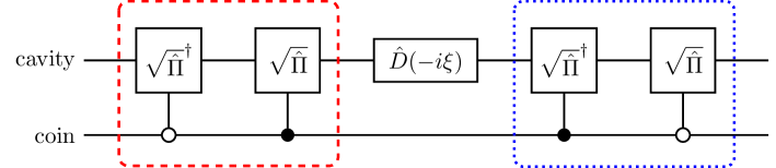
Figure 7: Circuit for implementing the controlled cavity displacement operation, where $\hat{\Pi}\equiv\exp(-i\pi\hat{a}^{\dagger}\hat{a})$ is the phase-space parity operator for the cavity mode. Here the controlled gates would enact cavity rotations depending on the coin qubit being in the state $|0\rangle$ (open circle) or the state $|1\rangle$ (filled circle). Notice that the gate combination in the red dashed box is the inverse of that in the blue dotted box.

To realize the controlled cavity displacement, here we will adopt a scheme based on conditional cavity phase shifts as shown in Fig. 7 Te16 . As explained in Sec. III in the main text, when the cavity-qubit coupling enters the strong dispersive regime the Jaynes-Cummings dynamics enables a conditional phase-space rotation of the cavity mode. For $\chi t=\pi/2$, it follows from (43) that we have the operation

$$e^{-i\frac{\pi}{2}\,\hat{a}^{\dagger}\hat{a}\otimes\hat{Z}}=\sqrt{\hat{\Pi}}\otimes|0\rangle\langle 0|+\sqrt{\hat{\Pi}}^{\dagger}\otimes|1\rangle\langle 1|\,,$$ (81)

where $\hat{\Pi}\equiv\exp(-i\pi\hat{a}^{\dagger}\hat{a})$ is the phase-space parity operator for the cavity mode. As in (43), here $|0\rangle$ and $|1\rangle$ stand for, respectively, the lower and upper qubit levels, which can be assigned to the coin states, say, as follows

$$|R\rangle\equiv|0\rangle\quad\mbox{and}\quad|L\rangle\equiv|1\rangle\,.$$ (82)

It is then easy to verify that the gate sequence in Fig. 7 would lead to

$$\hat{D}(-\xi)\otimes|0\rangle\langle 0|+\hat{D}(+\xi)\otimes|1\rangle\langle 1|=\left[\hat{I}\otimes|0\rangle\langle 0|+\hat{D}(+2\xi)\otimes|1\rangle\langle 1|\right]\hat{D}(-\xi)\,,$$ (83)

which furnishes the desired controlled cavity displacement operation. Notice that the pair of gates in the blue dotted box in Fig. 7 combine to enact the operation (81), while those in the red dashed box yield its inverse.

To realize the gate sequence of Fig. 7 experimentally, the unconditional cavity displacement $\hat{D}(-i\xi)$ can be carried out using a short unselective microwave pulse. For the conditional cavity rotation (81), as (43) suggests, free evolution of the dispersive Hamiltonian by a waiting time $t=\pi/2\chi$ will furnish the gate automatically Le13 ; Vl13 ; Le13b . Similarly, the inverse of (81) can be done by free evolution with a waiting time $t=3\pi/2\chi$, or by conjugating (81) with Pauli-$X$ gates for the coin qubit. Alternatively, the controlled cavity displacement can also be effected using a microwave driving field resonant with one of the qubit levels Te16 ; Vl13 ; Le13b . The resulting qubit-cavity dynamics will then induce cavity displacements conditioned on the qubit states. Nevertheless, this approach would require a longer gate operation time.

D.2 The biased coin-toss operation

We shall now explain how the biased coin-toss operation for QW-encoding can be achieved through realizing the corresponding positive operator-valued measure (POVM). To be specific, we will be considering the biased coin-toss $\hat{\cal B}_{D}$ of (40) for the dissipative QW-encoding. To construct a POVM for this operation, we start by noting that the corresponding measurement operator reads Wi10

$$\hat{M}_{D}\propto\left(|0\rangle\langle 0|+\frac{|1\rangle\langle+|}{\sqrt{2}}\right)\,,$$ (84)

where we have denoted the coin states as in (82), and hence

$$|D\rangle\equiv\frac{|0\rangle+|1\rangle}{\sqrt{2}}\equiv|+\rangle\,.$$ (85)

The effect operator for (84) is thus

$$\hat{F}_{D}=\hat{M}_{D}^{\dagger}\hat{M}_{D}\propto\left(|0\rangle\langle 0|+\frac{|+\rangle\langle+|}{2}\right)\,.$$ (86)

With these observations, we are then able to construct a properly normalized two-element POVM $\{\hat{F}_{1},\hat{F}_{2}\}$ for our purpose, which has the elements

$$\hat{F}_{1}=\sqrt{\frac{2}{3}}\left(|0\rangle\langle 0|+\frac{|+\rangle\langle+|}{2}\right)\quad\mbox{and}\quad\hat{F}_{2}=\sqrt{\frac{2}{3}}\left(|1\rangle\langle 1|+\frac{|-\rangle\langle-|}{2}\right)\,,$$ (87)

where $|-\rangle\equiv(|0\rangle-|1\rangle)/\sqrt{2}$, as usual. In realizations for the POVM (87), detection of $\hat{F}_{1}$ thus signals successful implementation of the biased coin-toss transformation (40).

According to Neumark’s theorem Pe93 , for any POVM in a state space, one can always realize it through orthogonal projective measurements in an extended state space. For the non-projective POVM (87) here, a systematic construction for such “Neumark extension” has been developed for photonic qubits AP05 , which has recently been extended to circuit architectures YB19 . To carry out the scheme, one starts by finding the singular-value decompositions (SVD’s) for the measurement operators $\{\hat{M}_{1},\hat{M_{2}}\}$ for the POVM (87), namely,

$$\hat{M}_{1} = \sqrt{\frac{2}{3}}\left(|0\rangle\langle 0|+\frac{1}{\sqrt{2}}|1\rangle\langle+|\right)=\sqrt{\frac{2}{3}}\left(\begin{array}[]{cc}1&0\\ \frac{1}{2}&\frac{1}{2}\\ \end{array}\right)\,,$$ (90)

$$\hat{M}_{2} = \sqrt{\frac{2}{3}}\left(|1\rangle\langle 1|+\frac{1}{\sqrt{2}}|0\rangle\langle-|\right)=\sqrt{\frac{2}{3}}\left(\begin{array}[]{cc}\frac{1}{2}&-\frac{1}{2}\\ 0&1\\ \end{array}\right)\,,$$ (93)

where the matrices are found with respect to the basis $\{|0\rangle,|1\rangle\}$. The results for the SVD’s are

$$\hat{M}_{i}=\hat{V}\hat{D}_{i}\hat{U}\,,\quad\mbox{$i=1,2$}\,,$$ (94)

where

$$\hat{V} = \frac{1}{\sqrt{10+2\sqrt{5}}}\left(\begin{array}[]{cc}-2&1+\sqrt{5}\\ 1+\sqrt{5}&2\\ \end{array}\right)\,,$$ (97)

$$\hat{U} = \frac{1}{\sqrt{10+4\sqrt{5}}}\left(\begin{array}[]{cc}-1&2+\sqrt{5}\\ 2+\sqrt{5}&1\\ \end{array}\right)\,,$$ (100)

$$\hat{D}_{1} = \frac{1}{2\sqrt{3}}\left(\begin{array}[]{cc}\sqrt{5}-1&0\\ 0&\sqrt{5}+1\\ \end{array}\right)\equiv\left(\begin{array}[]{cc}\cos\theta_{1}&0\\ 0&\cos\theta_{2}\\ \end{array}\right)\,,$$ (105)

$$\hat{D}_{2} = \frac{1}{2\sqrt{3}}\left(\begin{array}[]{cc}\sqrt{5}+1&0\\ 0&\sqrt{5}-1\\ \end{array}\right)\equiv\left(\begin{array}[]{cc}\sin\theta_{1}&0\\ 0&\sin\theta_{2}\\ \end{array}\right)\,.$$ (110)

Notice that although $\theta_{2}=\pi/2-\theta_{1}$ here, we keep both angles explicit in conformity with the notations of Ref. YB19 .

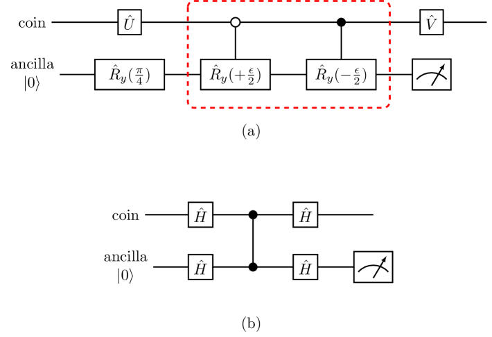
Figure 8: Circuits for implementing (a) the biased coin-toss transformation $\hat{\cal B}_{D}$ and (b) the fair coin-toss transformation $\hat{\cal C}_{D}$ for dissipative QW-encoding. For the controlled gates in the red dashed box in (a), the gates $\hat{R}_{y}(\pm\epsilon/2)$ would act on the ancilla qubit conditioned on the coin qubit being in the state $|0\rangle$ (open circle) or the state $|1\rangle$ (filled circle). In both panels, the measuring device stands for Pauli-$Z$ measurement for the ancilla qubit.

Following the scheme of Ref. YB19 , one can now construct a circuit for realizing the POVM (87) as shown in Fig. 8(a), where we have denoted the angle $\epsilon\equiv(\theta_{1}-\theta_{2})=\cos^{-1}(2/3)\simeq 48.19^{\circ}$ and the operator for single-qubit $y$-rotation by angle $\phi$ as

$$\hat{R}_{y}(\phi)\equiv e^{-i\hat{Y}\phi}$$ (111)

with $\hat{Y}$ the Pauli-$Y$ operator. Since both measurement operators $\hat{M}_{i}$ share the same unitary operator $\hat{V}$ for their SVD’s in (94), here we are able to simplify our circuit in comparison with that of Ref. YB19 . As one can verify, for an arbitrary coin state $|\psi_{c}\rangle$ and initial ancilla state $|0\rangle$, the circuit of Fig. 8(a) induces the following map prior to the ancilla measurement

$$|\psi_{c}\rangle|0\rangle\rightarrow\hat{M}_{1}|\psi_{c}\rangle|0\rangle+\hat{M}_{2}|\psi_{c}\rangle|1\rangle\,,$$ (112)

where $\hat{M}_{1}$, $\hat{M}_{2}$ are the measurement operators of (93). Therefore, when Pauli-$Z$ measurement on the ancilla yields outcome $|0\rangle$, it indicates that the biased coin-toss transformation (40) over the coin qubit has been implemented successfully.

Experimentally, the circuit in Fig. 8(a) for implementing the biased coin-toss should be accessible to current technologies with cQED systems We17 . A possible setup for this purpose is illustrated in the auxiliary part of Fig. 6, where a cavity bus resonator ($C_{2}$) is used to couple the coin (transmon) qubit ($Q_{c}$) and the ancilla (transmon) qubit ($Q_{a}$), and another cavity ($C_{3}$) is used to read out and reset the ancilla state. For the single-qubit unitaries in Fig. 8(a), they can be achieved by driving the transmon qubits with resonant microwave pulses Bl04 ; We17 . For the two-qubit controlled gates enclosed in the red dashed box, they are exactly the gates realized in the experiments of Ref. Gr13 . We note that this gate combination can be expressed as

$$\hat{R}_{x}\!\!\left(\!-\frac{\pi}{4}\right)\,\hat{C}_{Z}\!\!\left(\frac{\epsilon}{2}\right)\,\hat{R}_{x}\!\!\left(\!+\frac{\pi}{4}\right)\,,$$ (113)

where we have defined the conditional $z$-rotation

$$\hat{C}_{Z}(\phi)\equiv|0\rangle\langle 0|\otimes\hat{R}_{z}(\phi)+|1\rangle\langle 1|\otimes\hat{R}_{z}(-\phi)\,.$$ (114)

As in (111), here we have denoted $\hat{R}_{x}(\phi)\equiv e^{-i\hat{X}\phi}$ for $x$-rotation of the ancilla qubit and $\hat{R}_{z}(\phi)\equiv e^{-i\hat{Z}\phi}$ for its $z$-rotation, with $\hat{X}$ and $\hat{Z}$ the corresponding Pauli operators. In the experiment of Gr13 , the conditional $z$-rotation is realized by first transferring the state of the control qubit (in our case, the coin qubit) to the bus cavity. A photon-number dependent $z$-rotation over the target qubit (the ancilla qubit for us) is then enacted through free evolution of the dispersive Hamiltonian. After a waiting time, the cavity state is then transferred back to the control qubit, which completes the gate operation $\hat{C}_{Z}(\phi)$.

An alternate approach to realizing the conditional $z$-rotation (114) is to exploit the two-qubit higher excitation levels to generate tunable dynamical phase differences amongst the computational states Di09 . This is achieved by flux biasing one of the qubits, so that its transition frequency is brought to the proximity of an anti-level-crossing in the two-qubit spectrum. The corresponding time evolution thus results in the following effective evolution operator for the two-qubit computational states $\{|00\rangle,|01\rangle,|10\rangle,|11\rangle\}$ We17 ; Di09

$$\hat{U}\equiv|00\rangle\langle 00|+e^{i\phi_{01}}|01\rangle\langle 01|+e^{i\phi_{10}}|10\rangle\langle 10|+e^{i\phi_{11}}|11\rangle\langle 11|\,,$$ (115)

where $\phi_{ij}$ is the dynamical phase of level $|ij\rangle$, and $\phi_{11}=(\phi_{01}+\phi_{10}-\phi_{\zeta})$ with $\phi_{\zeta}$ adjustable through flux bias control. In the case with $\phi_{01}=\phi_{10}=\epsilon$ and $\phi_{\zeta}=2(\epsilon-\pi)$ (thus $\phi_{11}=2\pi$), we have from (115)

$$\hat{U}\mapsto e^{i\frac{\epsilon}{2}}\hat{C}_{Z}\!\!\left(\frac{\epsilon}{2}\right)\,,$$ (116)

which is the conditional $z$-rotation we wish to implement in (113) up to a global phase. And if we have $\phi_{01}=\phi_{10}=2\pi$ and $\phi_{\zeta}=3\pi$ (thus $\phi_{11}=\pi$), we then have Di09

$$\hat{U}\mapsto|0\rangle\langle 0|\otimes\hat{I}+|1\rangle\langle 1|\otimes\hat{Z}\,,$$ (117)

which furnishes the controlled-$Z$ gate. Therefore, by means of flux bias control, one can realize different two-qubit gates through the time-evolution operator (115). This flexibility makes the construction an ideal choice for implementing the coin-toss operations, not only for the biased one, but also for the fair one, which we shall now discuss.

D.3 The fair coin-toss operation

We now turn to the realization for the fair coin-toss $\hat{\cal C}_{D}$ of (17) for dissipative QW-encoding. Denoting the coin states as in (82) and (85) above, we see that the gate $\hat{\cal{C}}_{D}$ is simply the projector for the Pauli-$X$ eigenstate $|+\rangle$. The circuit for realizing this gate is thus well known (see, e.g., Ref. NC00 ) and is given in Fig. 8(b). It is easy to show that when the ancilla qubit is detected in the state $|0\rangle$, the coin state would be projected onto the state $|+\rangle$, implying successful implementation of the gate $\hat{\cal C}_{D}$.

To realize the circuit here experimentally, as discussed in the preceding subsection, the controlled-$Z$ gate can be implemented through flux bias control on one of the qubits. Therefore, along with microwave pulses enacting the Hadamard gates and Pauli-$Z$ measurement for the ancilla qubit, one would be able to furnish the desired fair coin-toss operation $\hat{\cal C}_{D}$ in accordance with the circuit in Fig. 8(b).

References

- (1) Nielsen, M.A., Chuang, I.L.: Quantum Computation and Quantum Information. Cambridge University Press, Cambridge (2000)
- (2) Castelvecchi, D.: Quantum computers ready to leap out of the lab in 2017. Nature 541, 9–10 (2017)
- (3) Lidar, D.A., Brun, T.A. (eds.): Quantum Error Correction. Cambridge University Press, Cambridge (2013)
- (4) Zhang, J., Braunstein, S.L.: Continuous-variable Gaussian analog of cluster states. Phys. Rev. A 73, 032318 (2006)
- (5) Menicucci, N.C., van Loock, P., Gu, M., Weedbrook, C., Ralph, T.C., Nielsen, M.A.: Universal quantum computation with continuous-variable cluster states. Phys. Rev. Lett. 97, 110501 (2006)
- (6) Menicucci, N.C.: Fault-tolerant measurement-based quantum computing with continuous-variable cluster states. Phys. Rev. Lett. 112, 120504 (2014)
- (7) Fukui, K., Tomita, A., Okamoto, A.: Analog quantum error correction with encoding a qubit into an oscillator. Phys. Rev. Lett. 119, 180507 (2017)
- (8) Fukui, K., Tomita, A., Okamoto, A., Fujii, K.: High-threshold fault-tolerant quantum computation with analog quantum error correction. Phys. Rev. X 8, 021054 (2018)
- (9) Gottesman, D., Kitaev, A., Preskill, J.: Encoding a qubit in an oscillator. Phys. Rev. A 64, 012310 (2001)
- (10) Travaglione, B.C., Milburn, G.J.: Preparing encoded states in an oscillator. Phys. Rev. A 66, 052322 (2002)
- (11) Pirandola, S., Mancini, S., Vitali, D., Tombesi, P.: Constructing finite-dimensional codes with optical continuous variables. Europhys. Lett. 68, 323–329 (2004)
- (12) Pirandola, S., Mancini, S., Vitali, D., Tombesi, P.: Continuous variable encoding by ponderomotive interaction. Eur. Phys. J. D 37, 283–290 (2006)
- (13) Pirandola, S., Mancini, S., Vitali, D., Tombesi, P.: Generating continuous variable quantum codewords in the near-field atomic lithography. J. Phys. B 39, 997–1009 (2006)
- (14) Vasconcelos, H.M., Sanz, L., Glancy, S.: All-optical generation of states for “Encoding a qubit in an oscillator”. Opt. Lett. 35, 3261–3263 (2010)
- (15) Brooks, P., Kitaev, A., Preskill, J.: Protected gates for superconducting qubits. Phys. Rev. A 87, 052306 (2013)
- (16) Terhal, B.M., Weigand, D.: Encoding a qubit into a cavity mode in circuit QED using phase estimation. Phys. Rev. A 93, 012315 (2016)
- (17) Motes, K.R., Baragiola, B.Q., Gilchrist, A., Menicucci, N.C.: Encoding qubits into oscillators with atomic ensembles and squeezed light. Phys. Rev. A 95, 053819 (2017)
- (18) Weigand, D.J., Terhal, B.M.: Generating grid states from Schrödinger-cat states without postselection. Phys. Rev. A 97, 022341 (2018)
- (19) Flühmann, C., Nguyen, T.L., Marinelli, M., Negnevitsky, V., Mehta, K., Home, J.P.: Encoding a qubit in a trapped-ion mechanical oscillator. Nature 566, 513–517 (2019)
- (20) Kempe, J.: Quantum random walks: An introductory overview. Contemp. Phys. 44, 307–327 (2003)
- (21) Manouchehri, K., Wang, J.: Physical Implementation of Quantum Walks. Springer-Verlag, Berlin (2014)
- (22) Braunstein, S.L., Pati, A.K. (eds.): Quantum Information with Continuous Variables. Kluwer, Dordrecht (2003)
- (23) Braunstein, S.L., van Loock, P.: Quantum information with continuous variables. Rev. Mod. Phys. 77, 513–577 (2005)
- (24) Ambainis, A., Bach, E., Nayak, A., Vishwanath, A., Watrous, J.: One-dimensional quantum walks. In: Proceedings of the Thirty-third Annual ACM Symposium on Theory of Computing, STOC ’01, pp. 37–49. ACM, New York (2001)
- (25) Kendon, V.: Decoherence in quantum walks – a review. Math. Struct. in Comp. Science 17, 1169–1220 (2007)
- (26) Glancy, S., Knill, E.: Error analysis for encoding a qubit in an oscillator. Phys. Rev. A 73, 012325 (2006)
- (27) Albert, V.V., Noh, K., Duivenvoorden, K., Young, D.J., Brierley, R.T., Reinhold, P., Vuillot, C., Li, L., Shen, C., Girvin, S.M., Terhal, B.M., Jiang, L.: Performance and structure of single-mode bosonic codes. Phys. Rev. A 97, 032346 (2018)
- (28) Vahlbruch, H., Mehmet, M., Danzmann, K., Schnabel, R.: Detection of 15 dB squeezed states of light and their application for the absolute calibration of photoelectric quantum efficiency. Phys. Rev. Lett. 117, 110801 (2016)
- (29) Cochrane, P.T., Milburn, G.J., Munro, W.J.: Macroscopically distinct quantum-superposition states as a bosonic code for amplitude damping. Phys. Rev. A 59, 2631–2634 (1999)
- (30) Leghtas, Z., Kirchmair, G., Vlastakis, B., Schoelkopf, R.J., Devoret, M.H., Mirrahimi, M.: Hardware-efficient autonomous quantum memory protection. Phys. Rev. Lett. 111, 120501 (2013)
- (31) Vlastakis, B., Kirchmair, G., Leghtas, Z., Nigg, S.E., Frunzio, L., Girvin, S.M., Mirrahimi, M., Devoret, M.H., Schoelkopf, R.J.: Deterministically encoding quantum information using 100-photon Schrödinger cat states. Science 342, 607–610 (2013)
- (32) Ofek, N., Petrenko, A., Heeres, R., Reinhold, P., Leghtas, Z., Vlastakis, B., Liu, Y., Frunzio, L., Girvin, S.M., Jiang, L., Mirrahimi, M., Devoret, M.H., Schoelkopf, R.J.: Extending the lifetime of a quantum bit with error correction in superconducting circuits. Nature 536, 441–445 (2016)
- (33) Blais, A., Huang, R.-S., Wallraff, A., Girvin, S.M., Schoelkopf, R.J.: Cavity quantum electrodynamics for superconducting electrical circuits: an architecture for quantum computation. Phys. Rev. A 69, 062320 (2004)
- (34) Girvin, S.M.: Circuit QED: superconducting qubits coupled to microwave photons. In: Devoret, M., Huard, B., Schoelkopf, R., Cugliandolo, L.F. (eds.) Quantum Machines: Measurement and Control of Engineered Quantum Systems, pp. 113-255. Oxford University Press, Oxford (2014)
- (35) Wendin, G.: Quantum information processing with superconducting circuits: a review. Rep. Prog. Phys. 80, 106001 (2017)
- (36) Schleich, W.P.: Quantum Optics in Phase Space. Wiley-VCH, Berlin (2001)
- (37) Haroche, S., Raimond, J.-M.: Exploring the Quantum–Atoms, Cavities, and Photons. Oxford University Press, Oxford (2006)
- (38) Majer, J., Chow, J.M., Gambetta, J.M., Koch, J., Johnson, B.R., Schreier, J.A., Frunzio, L., Schuster, D.I., Houck, A.A., Wallraff, A., Blais, A., Devoret, M.H., Girvin, S.M., Schoelkopf, R.J.: Coupling superconducting qubits via a cavity bus. Nature 449, 443–447 (2007)
- (39) DiCarlo, L., Chow, J.M., Gambetta, J.M., Bishop, L.S., Johnson, B.R., Schuster, D.I., Majer, J., Blais, A., Frunzio, L., Girvin, S.M., Schoelkopf, R.J.: Demonstration of two-qubit algorithms with a superconducting quantum processor. Nature 460, 240–244 (2009)
- (40) Strauch, F.W.: Connecting the discrete- and continuous-time quantum walks. Phys. Rev. A 74, 030301 (2006)
- (41) Leghtas, Z., Kirchmair, G., Vlastakis, B., Devoret, M.H., Schoelkopf, R.J., Mirrahimi, M.: Deterministic protocol for mapping a qubit to coherent state superpositions in a cavity. Phys. Rev. A 87, 042315 (2013)
- (42) Wiseman, H.M., Milburn, G.J.: Quantum Measurement and Control. Cambridge University Press, Cambridge (2010)
- (43) Peres, A.: Quantum Theory: Concepts and Methods. Kluwer, Dordrecht (1993)
- (44) Ahner, S.E., Payne, M.C.: General implementation of all possible positive-operator-value measurements of single-photon polarization states. Phys. Rev. A 71, 012330 (2005)
- (45) Yordanov, Y.S., Barnes, C.H.M.: Implementation of a general single-qubit positive operator-valued measure on a circuit-based quantum computer. Phys. Rev. A 100, 062317 (2019)
- (46) Groen, J.P., Ristè, D., Tornberg, L., Cramer, J., de Groot, P.C., Picot, T., Johansson, G., DiCarlo, L.: Partial-measurement backaction and nonclassical weak values in a superconducting circuit. Phys. Rev. Lett. 111, 090506 (2013)