Economics of carbon-dioxide abatement under an exogenous constraint on cumulative emissions

Abstract

The fossil-fuel induced contribution to further warming over the 21st century will be determined largely by integrated CO₂ emissions over time rather than the precise timing of the emissions, with a relation of near-proportionality between global warming and cumulative CO₂ emissions. This paper examines optimal abatement pathways under an exogenous constraint on cumulative emissions. Least cost abatement pathways have carbon tax rising at the risk-free interest rate, but if endogenous learning or climate damage costs are included in the analysis, the carbon tax grows more slowly. The inclusion of damage costs in the optimization leads to a higher initial carbon tax, whereas the effect of learning depends on whether it appears as an additive or multiplicative contribution to the marginal cost curve. Multiplicative models are common in the literature and lead to delayed abatement and a smaller initial tax. The required initial carbon tax increases with the cumulative abatement goal and is higher for lower interest rates. Delaying the start of abatement is costly owing to the increasing marginal abatement cost. Lower interest rates lead to higher relative costs of delaying abatement because these induce higher abatement rates early on. The fraction of business-as-usual emissions (BAU) avoided in optimal pathways increases for low interest rates and rapid growth of the abatement cost curve, which allows a lower threshold global warming goal to become attainable without overshoot in temperature. Each year of delay in starting abatement raises this threshold by an increasing amount, because the abatement rate increases exponentially with time.

Centre for Atmospheric and Oceanic Sciences and Divecha Centre for Climate Change, Indian Institute of Science, Bangalore, 560012, India (ashwin@fastmail.fm; ashwins@iisc.ac.in)

1 Introduction

Abatement of global warming requires reductions in emissions of carbon-dioxide (CO₂), with estimated costs of large-scale decarbonization varying substantially across studies and models (Manne and Richels (1993); Grubb (1993); Weyant (1993)), a major factor being baseline energy demand under “business as usual” (BAU) (Rogelj et al. (2015)). An important context of abatement is approximate proportionality between global warming from CO₂ and its cumulative emissions (Allen et al. (2009); Matthews et al. (2009)), and more generally that this relation is independent of emissions pathway (Herrington and Zickfeld (2014); Seshadri (2017a)). Such “path-independence” simplifies comparison of CO₂ emissions scenarios, requiring only that cumulative emissions be considered (Zickfeld et al. (2009); Bowerman et al. (2011)). In general, since global warming is not in equilibrium with radiative forcing owing to the slow climate response (Stouffer (2004); Held et al. (2010)), comparison of emissions scenarios invokes climate modeling uncertainties (Shine et al. (2005); Allen et al. (2016); Seshadri (2017b)) and this is where cumulative emissions accounting presents a major simplification for CO₂ (Matthews et al. (2012); Stocker et al. (2013)). In this case, path independence arises from the direct effects of changing cumulative emissions being an order of magnitude larger than effects of the slowly changing airborne fraction of excess CO₂, which can be understood in terms of corresponding timescales of evolution (Seshadri (2017a)).

Cumulative carbon budgets also raise new questions for analyses of mitigation pathways, given an exogenous constraint on cumulative emissions, in contrast with the effects of a Pigouvian tax (Pigou (1920)), i.e. a tax that internalizes the external damage costs of emissions. The evolution of such a tax must evolve according to the changing social cost of carbon (SCC) (Pearce (2003); Nordhaus (2017)), i.e. the discounted future global damages from the pulse emission of a ton of CO₂ . Since such a tax is meant to internalize the present value of the future costs of present emissions, the value of estimated SCC would determine the level of abatement. In contrast the scientific discussion about cumulative carbon budgets has examined decarbonization strategies achieving stringent global warming goals (e.g. Rogelj et al. (2011); Millar et al. (2017)). These do not directly reference the SCC, but are motivated by a precautionary approach to avoiding large but uncertain human and environmental consequences of failure (Meinshausen et al. (2009); Hoegh-Guldberg et al. (2018)). Moreover, although the effectiveness of the earlier Kyoto protocol is marred by limited scope (Shishlov et al. (2016)), growing evidence of the temperature-sensitivity of climate change impacts has animated rising ambition (Smith et al. (2009); Hoegh-Guldberg et al. (2018)), translating to difficult cumulative emissions goals (Meinshausen et al. (2009); Stocker (2013); Rhein et al. (2013)), now set in the context of the Paris Agreement seeking to hold “increase in the global average temperature to well below 2ï¿œC above pre-industrial levels and pursuing efforts to limit the temperature increase to 1.5ï¿œC above pre-industrial levels, recognizing that this would significantly reduce the risks and impacts of climate change” (UNFCCC (2015)).

Previous studies have considered economics of cumulative emissions abatement, including optimal paths that optimize a social welfare functional, as well as abatement expenditures under an exogenous constraint on cumulative emissions (Dietz and Venmans (2019); Emmerling et al. (2019); van der Ploeg and Rezai (2019)). These studies have undertaken far-reaching analyses of wide-ranging questions such as optimal temperatures (Dietz and Venmans (2019)), carbon price pathways (Dietz and Venmans (2019); Emmerling et al. (2019); van der Ploeg and Rezai (2019)), effect of damage costs (Dietz and Venmans (2019)), effects of discounting (Emmerling et al. (2019)), carbon budget overshoots (Emmerling et al. (2019)), inter-generational inequality aversion (van der Ploeg and Rezai (2019)), and exogenous technical progress (van der Ploeg and Rezai (2019)). The present paper focuses on abatement under an exogenous cumulative emissions constraint, extending the previous analyses to model BAU emissions, the effects of endogenous learning in addition to climate damages, and allowing economic growth and interest rates to vary with time. Prior authors have examined endogenous learning, starting with Arrow (1962), who modeled it as depending on cumulative investment and, although not a standard part of IAMs, endogenous learning has been studied in the CO₂ abatement context (e.g. Goulder and Mathai (2000); van der Zwaan et al. (2002); Wing (2006); Gillingham et al. (2008) ), although effects on optimizing pathways under a cumulative emissions constraint have not been examined. We also examine the effects of a delayed start to abatement. Cumulative emissions budgets might appear ambivalent for stringent climate policy, with delayed present abatement manageable via increases in future abatement. We examine the costs of delaying the onset of a global carbon tax and we show that the tradeoff between lower discounted future costs versus the need for a rapid transition resulting from a delay is limited once the time-value of money is factored into the optimal abatement pathways. The need for more rapid abatement following a delay drives its cost.

The present work examines cost abatement pathways and consequences for the carbon tax, assuming an exogenously determined end-of-century cumulative emissions goal. These pathways minimize abatement costs, either with or without endogenous learning, and we also consider the effects of including climate damages in the optimization. Where we address similar questions, the framework is similar to the aforementioned studies (Dietz and Venmans (2019); Emmerling et al. (2019)), wherein minimization gives rise to a two-point boundary value problem on cumulative abatement, which can solved for evolution of abatement rates. The corresponding evolution of a carbon tax in the context of a cumulative emissions constraint is examined, and the results correspond to those of the previous studies (Dietz and Venmans (2019); Emmerling et al. (2019)) for cases where endogenous learning’s effects are omitted. We consider applications to related questions: the influences on the initial value of the carbon tax, the effect of delaying abatement on growth in the present value of total expenditures as well as growth of the initial carbon tax, and the economics of avoiding overshoot in the global warming trajectory. Overshoot scenarios of the carbon budget have been considered previously by Emmerling et al. (2019). While the exogenous specification of cumulative emissions does not prevent overshoot of global warming compared to its value at the end of the time-horizon, limiting the magnitude of overshoot is important for averting impacts triggered by temperature thresholds (Smith et al. (2009); Hoegh-Guldberg et al. (2018)). Therefore we examine the constraints on the minimum amount of global warming that can be achieved without any overshoot and, given its approximate proportionality with cumulative emissions, avoiding overshoot of global warming requires net emissions to not be negative.

2 Models and methods

We are given an exogenous cumulative abatement goal $M_{tot}$, the total reduction in emissions compared to the business-as-usual scenario. Adopting a continuous-time formulation, with $t=0$ denoting the present, and $m\left(t\right)$ being the abatement rate in year $t$, the cumulative abatement $M\left(t\right)=\int_{0}^{t}m\left(s\right)ds$ must satisfy $M\left(T\right)=M_{tot}$ at the end of the time-horizon $t=T$. Following the notation typically used in variational calculus, abatement rate is henceforth denoted as $\dot{M}\left(t\right)\equiv\frac{dM\left(t\right)}{dt}$ instead of the above $m\left(t\right)$. The average cost of emissions abatement, in the absence of endogenous learning, is an increasing function $\gamma_{0}\left(\dot{M}\left(t\right)\right)$ of abatement rate, assuming that each year the cheaper abatements are undertaken first. Previous authors have shown evidence in a number of sectors for cost reductions depending on cumulative production (“endogenous learning” or “learning by doing”) (Rubin et al. (2004); Nagy et al. (2013)).With endogenous learning, the average cost is lowered progressively as cumulative abatement $M\left(t\right)$ grows, so that in general the average cost is $\gamma\left(\dot{M}\left(t\right),M\left(t\right)\right)$. Climate damages are modeled as an increasing function of global warming.

2.1 Business-as-usual emissions

The business as usual (BAU) emissions rate depends on global GDP $G\left(t\right)$ and global emissions intensity $\mu\left(t\right)$ of CO₂ as $\dot{E}_{BAU}\left(t\right)=G\left(t\right)\mu\left(t\right)$. Its growth rate depends on the global income elasticity of emissions $\theta$ since, over time-interval $\triangle t$ , the relative change in BAU emissions rate is $\triangle\dot{E}_{BAU}/\dot{E}_{BAU}=\theta\triangle G/G$. Thus, assuming exogenous GDP growth rate $r\left(t\right)=\triangle G\left(t\right)/G\left(t\right)$,emissions intensity under BAU declines at the rate $-\frac{1}{\mu}\frac{d\mu}{dt}=\left(1-\theta\right)\frac{r}{1+r}$ (Appendix 1). Since we can approximate $1/\left(1+r\right)\cong 1$, the emissions intensity under BAU can be described by $\mu\left(t\right)=\mu\left(0\right)e^{\left(\theta-1\right)R\left(t\right)}$ where $R\left(t\right)=\int_{0}^{t}r\left(s\right)ds$ is the integrated GDP growth rate and with the GDP growing as $G\left(t\right)=G\left(0\right)e^{R\left(t\right)},$the annual emissions rate under BAU is

$$\dot{E}_{BAU}\left(t\right)=\dot{E}_{BAU}\left(0\right)e^{\theta R\left(t\right)}$$ (1)

where we have allowed for time-varying $r$ but assume constant $\theta$. Across nations, the income elasticity of emissions varies considerably, depending on the pattern of economic growth, being generally smaller for richer economies (Webster et al. (2008)) and thus liable to decrease as economies develop.

2.2 Abatement cost model in the absence of endogenous learning

The average cost of emissions abatement is an increasing function of the abatement rate

$$\gamma_{0}\left(\dot{M}\left(t\right)\right)=c_{0}+c_{1}\left(\frac{\dot{M}\left(t\right)}{\dot{M}_{max}\left(t\right)}\right)^{c_{2}}$$ (2)

where $c_{1}>0$ and $c_{2}>0$, but the intercept $c_{0}$ can be negative to reflect the availability of negative-cost techniques. $\dot{M}_{max}\left(t\right)$ describes the horizontal scale of the abatement graph, at which average cost is fixed at $c_{0}+c_{1}$, which we take as equal to the BAU emissions $\dot{M}_{max}\left(t\right)=\dot{E}_{BAU}\left(t\right)$. As BAU emissions grow, abatement possibilities are assumed to expand proportionally. This also leads to the result that the abatement cost remains constant in the absence of policy-induced decarbonization or exogenous cost reductions, in line with models such as DICE (Nordhaus and Sztorc (2013)). Higher emissions reductions than $\dot{E}_{BAU}\left(t\right)$ are possible, being in the realm of net-negative emissions, with resulting average costs following Eq. (2) exceeding $c_{0}+c_{1}$. The model parallels prior approaches based on the marginal abatement cost, which is taken to be some power of the emissions reductions relative to BAU, e.g. Emmerling et al. (2019). It assumes that abatement possibilities are independent of the past history of mitigation, depending only on the BAU pathway of emissions.

2.3 Endogenous learning model

Only learning by doing is modeled, not exogenous learning with time, influencing the average cost as

$$\gamma\left(\dot{M}\left(t\right),M\left(t\right)\right)=\left(\gamma_{0}\left(\dot{M}\left(t\right)\right)-f\left(M\left(t\right)\right)\right)h\left(M\left(t\right)\right)$$ (3)

where $\gamma_{0}\left(\dot{M}\left(t\right)\right)$ describes the cost curve in the absence of learning, and the terms $f\left(M\left(t\right)\right)$ and $h\left(M\left(t\right)\right)$ are introduced to admit the different possibilities: learning shifts the cost curve down, scales it down, or does both. If there is only an additive term, then $f\left(M\left(t\right)\right)\geq 0$ and is increasing in $M\left(t\right)$, while $h\left(M\left(t\right)\right)=1$ and is fixed. If there is only a multiplicative term, then $f\left(M\left(t\right)\right)=0$ and is fixed while $h\left(M\left(t\right)\right)$, satisfying $0<h\left(M\left(t\right)\right)\leq 1$, is a decreasing function of cumulative abatement. The functions must satisfy $f\left(0\right)=0$ and $h\left(0\right)=1$. For example, an additive effect might take form $f\left(M\left(t\right)\right)=c_{f}M\left(t\right)$ with $c_{f}>0$ and $h\left(M\left(t\right)\right)=1$. A multiplicative effect could be $h\left(M\left(t\right)\right)=e^{-M\left(t\right)/M_{h}}$ with constant parameter $M_{h}>0$. In contrast to this decreasing exponential model, a power-law model suggested by the literature (Rubin et al. (2004); Nagy et al. (2013)) has form $h\left(M\left(t\right)\right)=\left(M\left(t\right)/M\left(t=0\right)\right)^{-b}$ with necessarily $M\left(t=0\right)>0$ . Any combination of the above effects is also possible.

2.4 Climate damages model

Climate damages are modeled as a fraction of GDP

$$D\left(t\right)=d\left(t\right)G\left(t\right)$$ (4)

where damage fraction $d\left(t\right)$ is increasing in global warming $\triangle T\left(t\right)$, which in turn is proportional to cumulative emissions

$$\triangle T\left(t\right)=\alpha E\left(t\right)$$ (5)

with $\alpha$ being the “transient climate response to cumulative carbon emissions” (TCRE) (Matthews et al. (2018)). Treating the damage fraction as a function of the temperature at time $t$ is conventional, but neglects important factors such as delayed impacts of sea-level rise and lasting impacts of extreme events. Cumulative emissions is measured from preindustrial time $-t_{PI}$

$$E\left(t\right)=\int_{-t_{PI}}^{0}\dot{E}\left(s\right)ds+\int_{0}^{t}\dot{E}\left(s\right)ds$$ (6)

and, since the emissions rate is

$$\dot{E}\left(t\right)=\dot{E}_{BAU}\left(t\right)-\dot{M}\left(t\right)$$ (7)

where $\dot{E}_{BAU}\left(t\right)$ is the rate under “business as usual” (BAU), we obtain for cumulative emissions

$$E\left(t\right)=E_{BAU}\left(t\right)-M\left(t\right)$$ (8)

in terms of $E_{BAU}\left(t\right)$, the cumulative emissions under BAU. With respect to cumulative abatement, global warming is $\triangle T\left(t\right)=\alpha\left\{E_{BAU}\left(t\right)-M\left(t\right)\right\}$ and we subsequently treat alternate formulations of damage function $d\left(\triangle T\right).$

2.5 Constrained optimization framework

The analysis of this paper is founded on pathways minimizing the present value of abatement costs, or sum of total abatement and damage costs. Since $\gamma\left(t\right)$ is average cost per unit of abatement in year $t$, total abatement cost in a year is

$$A\left(M\left(t\right),\dot{M}\left(t\right)\right)=\gamma\left(t\right)\dot{M}\left(t\right)=\left(\gamma_{0}\left(\dot{M}\left(t\right)\right)-f\left(M\left(t\right)\right)\right)h\left(M\left(t\right)\right)\dot{M}\left(t\right)$$ (9)

Similarly, the damage cost is given by Eq. (4). We must minimize the present value of these costs, between $t=0$ and $t=T$, subject to the aforementioned constraint on cumulative abatement $\int_{0}^{T}\dot{M}\left(s\right)ds=M_{tot}.$ At risk-free interest rate $i\left(t\right)$, the present value of the cost is

$$C_{total}=\int_{0}^{T}e^{-I\left(t\right)}C\left(t,M\left(t\right),\dot{M}\left(t\right)\right)dt$$ (10)

where

$$C\left(t,M\left(t\right),\dot{M}\left(t\right)\right)=\left(c_{0}+c_{1}\left(\frac{\dot{M}\left(t\right)}{\dot{M}_{max}\left(t\right)}\right)^{c_{2}}-f\left(M\left(t\right)\right)\right)h\left(M\left(t\right)\right)\dot{M}\left(t\right)\\ +d\left(M\left(t\right)\right)G\left(t\right)$$ (11)

is the sum of abatement and damage costs and $I\left(t\right)=\int_{0}^{t}i\left(s\right)ds$ is the cumulative interest rate at time $t$. Minimizing the functional in Eq. (10) subject to constraint on cumulative abatement, for fixed time-horizon $T$, involves finding a solution to the Euler-Lagrange equation (Appendix 2)

$$\frac{\partial g}{\partial M}+\lambda\frac{\partial\dot{M}}{\partial M}=\frac{d}{dt}\left(\frac{\partial g}{\partial\dot{M}}+\lambda\frac{\partial\dot{M}}{\partial\dot{M}}\right)$$ (12)

where

$$g\left(t,M\left(t\right),\dot{M}\left(t\right)\right)=e^{-I\left(t\right)}C\left(t,M\left(t\right),\dot{M}\left(t\right)\right)$$ (13)

is the integrand in Eq. (10). Tables 1 and 2 list some of the frequently used emissions and climate parameters, and economic parameters, respectively.

Table 1: Emissions and climate parameters

Symbol	Description	Units
$E\left(t\right)$	cumulative emissions of CO2	Gton
$M\left(t\right)$	cumulative abatement of CO2	Gton
$\dot{M}\left(t\right)$	abatement rate	Gton year$-1$
$\dot{M}_{max}\left(t\right)$	maximum abatement rate, equal to BAU emissions	Gton year$-1$
$r_{BAU}\left(t\right)$	growth rate of BAU emissions	year$-1$
$\triangle T\left(t\right)$	global warming from CO2	K
$\alpha$	transient climate response to cumulative carbon emissions (TCRE)	K Gton$-1$
$M_{tot}$	cumulative abatement	Gton

Table 2: Economics parameters

Symbol	Description	Units
$P$	carbon tax	$\$$ ton$-1$
$i\left(t\right)$	discount rate	year$-1$
$I\left(t\right)$	cumulative interest rate	dimensionless
$\theta$	income elasticity of emissions	dimensionless
$\gamma_{0}\left(\dot{M}\left(t\right),M\left(t\right)\right)$	average cost of abatement without learning	trillion $ Gton$-1$
$\gamma\left(\dot{M}\left(t\right),M\left(t\right)\right)$	average cost of abatement with learning	trillion $ Gton$-1$
$\beta\left(\dot{M}\left(t\right),M\left(t\right)\right)$	marginal cost of abatement with learning	trillion $ Gton$-1$
$A\left(t\right)$	abatement cost in year $t$	trillion $
$c_{0}$	intercept of average cost function	trillion $ Gton$-1$
$c_{1}$	coefficient of average cost function	trillion $ Gton$-1$
$c_{2}$	exponent of average cost function	dimensionless
$G\left(t\right)$	global GDP	trillion $
$d\left(t\right)$	climate damage fraction	dimensionless
$D\left(t\right)$	climate damage cost	trillion $
$T_{0}$	reference global warming for power-law damage-fraction	$10$ K
$d_{0}$	power-law damage fraction at $\triangle T=T_{0}$	dimensionless
$d_{1}$	exponent of power-law damage function	dimensionless
$d_{2}$	coefficient of logistic damage function	dimensionless
$E_{D}$	parameter for logistic damage function	Gton
$f\left(M\left(t\right)\right)$	additive learning	trillion $ Gton$-1$
$h\left(M\left(t\right)\right)$	multiplicative learning	dimensionless
$M_{h}$	parameter for exponential model of learning	Gton
$-b$	exponent of power-law model of learning	dimensionless
$c_{f}$	coefficient for additive model of learning	trillion $ Gton$-2$

3 Results

3.1 Optimal abatement rate

Using Eqs. (11) and (13), and simplifying (Appendix 3), the Euler-Lagrange Eq. (12) for the evolution of the abatement rate $\dot{M}\left(t\right)$ becomes

$$c_{1}c_{2}\left(c_{2}+1\right)\left(\frac{\dot{M}\left(t\right)}{\dot{M}_{max}\left(t\right)}\right)^{c_{2}}\frac{\ddot{M}\left(t\right)}{\dot{M}\left(t\right)}=i\left(t\right)\left\{c_{0}+c_{1}\left(c_{2}+1\right)\left(\frac{\dot{M}\left(t\right)}{\dot{M}_{max}\left(t\right)}\right)^{c_{2}}-f\left(M\left(t\right)\right)\right\}\\ +c_{1}c_{2}\left(c_{2}+1\right)\left(\frac{\dot{M}\left(t\right)}{\dot{M}_{max}\left(t\right)}\right)^{c_{2}}r_{BAU}\left(t\right)-\frac{c_{1}c_{2}}{\dot{M}_{max}^{c_{2}}\left(t\right)}\dot{M}\left(t\right)^{c_{2}+1}\frac{h^{\prime}\left(M\left(t\right)\right)}{h\left(M\left(t\right)\right)}+d^{\prime}\left(M\left(t\right)\right)\frac{G\left(t\right)}{h\left(M\left(t\right)\right)}$$ (14)

where $r_{BAU}\left(t\right)=\frac{1}{\dot{M}_{max}\left(t\right)}\left\{\frac{d}{dt}\dot{M}_{max}\left(t\right)\right\}=\theta r\left(t\right)$ is the growth rate of BAU emissions. This 2^nd-order equation in $M\left(t\right)$ requires two boundary values. At the present time when abatement is to begin, we have $M\left(t=0\right)=0$, in addition to cumulative abatement $M\left(t=T\right)=M_{tot}$. The parameters appearing in Eq. (14), along with these boundary conditions, uniquely prescribe the abatement pathway. We assume henceforth that average costs are increasing, i.e. $c_{1}$ and $c_{2}$ are positive; for, if average cost function were constant, with either $c_{1}$ or $c_{2}$ being equal to zero, we obtain an algebraic equation in $M\left(t\right)$, which in general is not soluble.

Let us consider the influences on evolution of abatement rate $\dot{M}\left(t\right)$ in Eq. (14), noting that $\frac{\ddot{M}\left(t\right)}{\dot{M}\left(t\right)}$ on the left describes its growth rate.

• A positive interest rate $i\left(t\right)>0$ induces late abatement by increasing the growth rate of $\dot{M}\left(t\right)$.

• Economic growth leads to future emissions growth and expansion of abatement possibilities, through the term in $r_{BAU}\left(t\right)$. This induces delayed abatement in the optimal solution, involving larger growth rate of $\dot{M}\left(t\right)$ if the GDP growth rate is higher.

• Without counting learning or damages, the horizontal position in the MAC, relative to maximum abatement rate, has a particularly simple form. Writing

  $$\sigma\left(t\right)=\frac{\dot{M}\left(t\right)}{\dot{M}_{max}\left(t\right)}$$ (15)

  which equals one when the annual emissions rate is exactly zero, its growth rate is

  $$\frac{1}{\sigma\left(t\right)}\frac{d\sigma\left(t\right)}{dt}=\frac{i\left(t\right)}{c_{2}}$$ (16)

• If the interest rate is positive, the presence of an additive model of learning with $f\left(M\left(t\right)\right)>0$ induces early abatement by decreasing the growth rate of $\dot{M}\left(t\right)$.

• In contrast the multiplicative model of learning with $h^{\prime}\left(M\left(t\right)\right)<0$ induces late abatement, regardless of the value of the interest rate.

• Climate damages induce early abatement, since $d^{\prime}\left(M\left(t\right)\right)<0$, with higher initial abatement rate followed by smaller growth rate of $\dot{M}\left(t\right)$.

3.2 Effects of the learning model

The basic distinction pertaining to the endogenous learning model is whether it appears as an additive or multiplicative contribution in the abatement cost function. An additive model causes early abatement in the presence of non-zero interest rate, whereas a multiplicative model induces late abatement regardless of time-valuation.

As show in Appendix 4, the marginal abatement cost (MAC) corresponding to our average cost model in Eq. (3) is

$$\beta\left(M,\dot{M}\right)=\left\{c_{0}+\frac{\left(c_{2}+1\right)c_{1}}{\dot{M}_{max}^{c_{2}}}\dot{M}^{c_{2}}-f\left(M\right)\right\}h\left(M\right)$$ (17)

and the additive learning term $-f\left(M\left(t\right)\right)$, being negative, reduces marginal cost by the same amount for all values of abatement rate, thus effecting a downward shift in the MAC curve. In contrast multiplication by $h\left(M\left(t\right)\right)$ pivots the MAC downward, reducing it by the same factor for all values of $\dot{M}$.

The effect of the additive model on growth rate of $\dot{M}\left(t\right)$ can be written as

$$c_{1}c_{2}\left(c_{2}+1\right)\left(\frac{\dot{M}\left(t\right)}{\dot{M}_{max}\left(t\right)}\right)^{c_{2}}\frac{\ddot{M}\left(t\right)}{\dot{M}\left(t\right)}=i\left(t\right)\frac{\beta\left(M\left(t\right),\dot{M}\left(t\right)\right)}{h\left(M\left(t\right)\right)}$$ (18)

where the effect of a positive $f\left(M\right)$ on the MAC has been taken into account in Eq. (17), and since it lowers the MAC $\beta\left(M\left(t\right),\dot{M}\left(t\right)\right)$ its effect is to moderate the growth rate of abatement without making it negative. Generally it cannot induce higher abatement rates early on.

The multiplicative term appears on the right as

$$-\frac{c_{1}c_{2}}{\dot{M}_{max}^{c_{2}}\left(t\right)}\dot{M}\left(t\right)^{c_{2}+1}\frac{h^{\prime}\left(M\left(t\right)\right)}{h\left(M\left(t\right)\right)}$$ (19)

and, since $h^{\prime}\left(M\right)<0$ the net contribution of the learning model to the right side is positive, with its effect being to increase emissions rate with time. This is opposite to the effect of the additive model, furthermore it manifests independently of the interest rate. Endogenous learning through the multiplicative term $h\left(N\right)$ is like discounting in time, reducing marginal costs by a common factor for all values of $\dot{M}\left(t\right)$, with the difference that in one case the reduction is a function of $M\left(t\right)$ whereas in the other directly of $t$. Therefore it is hardly surprising that such a learning model induces delayed abatement compared to the no-learning case.

As for the additive model, recall that its effect only occurs for non-zero interest rate. The corresponding term $f\left(M\right)$ in Eq. (14) is multiplied by $i\left(t\right)$, so the effect vanishes for zero interest rate. This much is obvious from the equation, but the underlying reasons are instructive and discussed in Appendix 5. There it is shown that in the absence of discounting, the variational problem reduces to minimizing a convex functional. From Jensen’s inequality this is solved by the expectation of the abatement rate, which is in fact the constant-rate trajectory.

4 Applications

4.1 Evolution of the carbon tax

How should the carbon tax evolve in order to induce the abatement rates that would minimize the present value of costs? Since a carbon tax of $P$ induces abatement activities whose marginal cost $\beta\left(M,\dot{M}\right)\leq P$, the evolution of the marginal abatement cost indicates this, and from Eqs. (14) and (17), the carbon-tax growth rate

$$\frac{dP\left(t\right)}{dt}=i\left(t\right)P\left(t\right)+\left\{\gamma\left(\dot{M}\left(t\right),M\left(t\right)\right)\frac{h^{\prime}\left(M\left(t\right)\right)}{h\left(M\left(t\right)\right)}-f^{\prime}\left(M\left(t\right)\right)h\left(M\left(t\right)\right)\right\}\dot{M}\left(t\right)\\ +d^{\prime}\left(M\left(t\right)\right)G\left(t\right)$$ (20)

comprises effects of the interest rate, endogenous learning, and economic damages from climate change. In the absence of learning and damages, the carbon tax growth $\frac{dP}{dt}=iP$ follows Hotelling’s rule regarding rent-extraction from nonrenewable resources (Hotelling (1931)), and parallels prior analyses (Dietz and Venmans (2019); Emmerling et al. (2019)), and Eq. (20) extends its validity to time-varying interest rate. Endogenous learning reduces the growth rate, with $h^{\prime}/h$ and $-f^{\prime}$ both being negative. Limiting damage costs in addition to meeting the cumulative emissions constraint necessitates higher taxes earlier on, and subsequent lower growth-rates of the carbon tax, and this is quantified by $d^{\prime}\left(M\right)<0$.

4.2 Cost of delaying abatement

The IPCC, in its 2013 assessment, acknowledged the lessons of proportionality between CO₂ induced global warming and cumulative emissions for carbon budgets: “The ratio of GMST [Global Mean Surface Temperature] change to total cumulative anthropogenic carbon emissions is relatively constant and independent of the scenario, but is model dependent, as it is a function of the model cumulative airborne fraction of carbon and the transient climate response. For any given temperature target, higher emissions in earlier decades therefore imply lower emissions by about the same amount later on” (Stocker et al. (2013)). The last statement might be interpreted to mean that a delay in starting abatement can be compensated by more stringent abatement in the future, but this would be expensive owing to increasing marginal costs of abatement.

What is the monetary cost of delaying abatement in the model, assuming that the optimal emissions pathway is followed? Imagine that abatement commences at $t=N$ years, where $0\leq N<T$. In the absence of endogenous learning, the present value of the abatement cost is

$$C_{total}=c_{1}\int_{N}^{T}e^{-I\left(t\right)}\sigma\left(t\right)^{c_{2}+1}\dot{M}_{max}\left(t\right)dt$$ (21)

assuming zero intercept $c_{0}=0$, and using Eqs. (2) and (15). Since $\dot{M}_{max}\left(t\right)$ is set equal to the BAU emissions, which grows at $\theta r\left(t\right)$, the optimal solution has $\sigma\left(t\right)$ growing at the rate $i\left(t\right)/c_{2}$, and the initial abatement rate is constrained by the cumulative constraint $\int_{N}^{T}\dot{M}\left(t\right)dt=M_{tot},$ integration yields

$$C_{total}=c_{1}\left(\frac{M_{tot}}{\dot{M}_{max}\left(0\right)}\right)^{c_{2}+1}\dot{M}_{max}\left(0\right)\frac{1}{\left\{\int_{N}^{T}e^{I\left(t\right)/c_{2}+\theta R\left(t\right)}dt\right\}^{c_{2}}}$$ (22)

as shown in Appendix 6. The last term increases with delayed starting year $N$, corresponding to starting farther along the marginal cost curve to meet the cumulative abatement constraint. Thus, a one-year delay in mitigation leads to relative growth of total cost’s present value

$$\frac{1}{C_{total}}\frac{\partial C_{total}}{\partial N}=c_{2}\frac{e^{I\left(N\right)/c_{2}+\theta R\left(N\right)}}{\int_{N}^{T}e^{I\left(t\right)/c_{2}+\theta R\left(t\right)}dt}$$ (23)

and for the special case of constant rate of interest and GDP growth at $i$ and $r$ respectively, this becomes

$$\frac{1}{C_{total}}\frac{\partial C_{total}}{\partial N}=c_{2}\left(\frac{i}{c_{2}}+\theta r\right)\frac{e^{\left(\frac{i}{c_{2}}+\theta r\right)N}}{e^{\left(\frac{i}{c_{2}}+\theta r\right)T}-e^{\left(\frac{i}{c_{2}}+\theta r\right)N}}$$ (24)

Our time-horizons in climate change mitigation typically specify end-of-century goals, so we stipulate that $T$ is long and therefore:

• if $N$ is small, $\frac{1}{C_{total}}\frac{\partial C_{total}}{\partial N}\approx\frac{c_{2}\left(\frac{i}{c_{2}}+\theta r\right)}{e^{\left(\frac{i}{c_{2}}+\theta r\right)T}}$

• whereas if $N$ is large, approaching $T$, $\frac{1}{C_{total}}\frac{\partial C_{total}}{\partial N}\approx\frac{c_{2}}{T-N}$

Evidently, delay in the start of mitigation (i.e. starting onto the optimal abatement trajectory) is costly in present-value terms because of increasing marginal costs of abatement. Such a delay entails higher abatement rates in the future, leading to higher costs.

The growth rate of the present value of abatement costs due to each year of delay in mitigation is independent of the abatement level, but depends on the time-horizon and the shape of the MAC. Delaying abatement is more costly if $c_{2}$ is higher, because rapid rise in the MAC requires higher initial abatement rates to limit future growth in costs. In contrast, assuming small $N$, delaying abatement is expensive but less so for high GDP growth or large interest rate, because these conditions lead to smaller starting abatement rates. Delay becomes more costly if the time-horizon is short. As the starting year for mitigation $N$ approaches $T-1$, the present-value of abatement cost grows at an increasing rate approaching $c_{2}$.

4.3 Initial carbon tax

How does such a delay in starting abatement influence the initial carbon tax necessary? The cumulative abatement constraint, without counting learning or damages, becomes (Appendix 6)

$$M_{tot}=\int_{N}^{T}\dot{M}\left(t\right)dt=\dot{M}\left(N\right)e^{-I\left(N\right)/c_{2}}e^{-\theta R\left(N\right)}\int_{N}^{T}e^{I\left(t\right)/c_{2}+\theta R\left(t\right)}dt$$ (25)

and using $\dot{M}_{max}\left(N\right)=\dot{M}_{max}\left(0\right)e^{\theta R\left(N\right)}$, the position along the MAC curve $\sigma\left(N\right)=\dot{M}\left(N\right)/\dot{M}_{max}\left(N\right)$ at the start of abatement is

$$\sigma\left(N\right)=\frac{M_{tot}}{\dot{M}_{max}\left(0\right)}\frac{e^{I\left(N\right)/c_{2}}}{\int_{N}^{T}e^{I\left(t\right)/c_{2}+\theta R\left(t\right)}dt}$$ (26)

which grows with $N$, so meeting a cumulative abatement following a delay requires one to start farther along the curve. This gives initial marginal cost, from Eq. (17), equal to $\beta\left(N\right)=c_{1}\left(c_{2}+1\right)\sigma\left(N\right)^{c_{2}}$ so the starting carbon tax must be

$$P\left(N\right)=c_{1}\left(c_{2}+1\right)\left(\frac{M_{tot}}{\dot{M}_{max}\left(0\right)}\right)^{c_{2}}\frac{e^{I\left(N\right)}}{\left\{\int_{N}^{T}e^{I\left(t\right)/c_{2}+\theta R\left(t\right)}dt\right\}^{c_{2}}}$$ (27)

As before, we consider effects of delayed abatement

$$\frac{1}{P}\frac{\partial P}{\partial N}=i\left(N\right)+c_{2}\frac{e^{I\left(N\right)/c_{2}+\theta R\left(N\right)}}{\int_{N}^{T}e^{I\left(t\right)/c_{2}+\theta R\left(t\right)}dt}$$ (28)

which is similar to Eq. (23), but with addition of Hotelling’s growth-rate $i\left(t\right)$. For constant $r$ and $i$, the corresponding limiting cases for long time-horizon $T$ are:

• $N$ small, $\frac{1}{P}\frac{\partial P}{\partial N}\approx i+\frac{c_{2}\left(\frac{i}{c_{2}}+\theta r\right)}{e^{\left(\frac{i}{c_{2}}+\theta r\right)T}}$

• whereas $N$ large, approaching $T$, $\frac{1}{P}\frac{\partial P}{\partial N}\approx i+\frac{c_{2}}{T-N}$

and the growth of the tax has a contribution from the Hotelling rate $i\left(t\right)$. Additionally each year’s delay in implementation gives rise to a further increase, owing to increasing marginal costs.

4.4 Economics of avoiding overshoot

Given proportionality between global warming and cumulative emissions, overshoot in CO₂’s warming contribution generally corresponds to net negative emissions. Scenarios avoiding overshoot therefore must have positive but declining emissions for $t<T$, so that $\sigma\left(t\right)<1$. The optimal pathways generally have $\sigma\left(t\right)$ growing in time, so we must only consider the constraint $\sigma\left(T\right)<1$ for avoiding an overshoot. Since the position along the abatement curve grows, without considering learning or damages, at $\sigma\left(T\right)=\sigma\left(N\right)e^{\int_{N}^{T}i\left(t\right)/c_{2}dt}$, we obtain from Eq. (61) in Appendix 6

$$\sigma\left(T\right)=\frac{M_{tot}}{\dot{M}_{max}\left(0\right)}\frac{e^{I\left(T\right)/c_{2}}}{\int_{N}^{T}e^{I\left(t\right)/c_{2}+\theta R\left(t\right)}dt}$$ (29)

Furthermore, in the absence of net negative emissions, future global warming is roughly proportional to future cumulative emissions via the TCRE $\alpha$, so that $\triangle T_{fut}=\alpha\left\{E_{BAU,fut}\left(T\right)-M_{tot}\right\}$. Future cumulative emissions under BAU is simply $E_{BAU,fut}\left(T\right)=\dot{M}_{max}\left(0\right)\int_{0}^{T}e^{\theta R\left(t\right)}dt$. Hence

$$\frac{M_{tot}}{\dot{M}_{max}\left(0\right)}=\int_{0}^{T}e^{\theta R\left(t\right)}dt-\frac{\triangle T_{fut}}{\alpha\dot{M}_{max}\left(0\right)}$$ (30)

and substituting in Eq. (29), the constraint $\sigma\left(T\right)<1$ for avoiding overshoot is

$$\frac{\triangle T_{fut}}{\alpha\dot{M}_{max}\left(0\right)}>\int_{0}^{T}e^{\theta R\left(t\right)}dt-\frac{\int_{N}^{T}e^{I\left(t\right)/c_{2}+\theta R\left(t\right)}dt}{e^{I\left(T\right)/c_{2}}}=\frac{\triangle T_{fut}^{*}}{\alpha\dot{M}_{max}\left(0\right)}$$ (31)

providing a lower bound $\triangle T_{fut}^{*}$ on future global warming from CO₂ attainable without overshoot, assuming an optimal pathway is being followed. Moreover, each year of delay in starting mitigation causes increase in this minimum attainable temperature

$$\frac{\partial\triangle T_{fut}^{*}}{\partial N}=\alpha\dot{M}_{max}\left(0\right)e^{-\int_{N}^{T}\frac{i\left(t\right)}{c_{2}}dt+\theta R\left(N\right)}>0$$ (32)

with the marginal effects of each subsequent year of delay rising as $\partial^{2}\triangle T_{fut}^{*}/\partial N^{2}=\left\{\frac{i}{c_{2}}\left(N\right)+\theta r\left(N\right)\right\}\frac{\partial\triangle T_{fut}^{*}}{\partial N}>0$, as long as $\frac{i}{c_{2}}+\theta r>0$. Hence, each year of delay makes it increasingly difficult to meet global warming goals without overshoot. For constant $i$ and $r$

$$\triangle T_{fut}^{*}=\alpha\dot{M}_{max}\left(0\right)\left\{\frac{e^{\theta rT}-1}{\theta r}-\frac{e^{\theta rT}}{\frac{i}{c_{2}}+\theta r}\left(1-e^{-\left(\frac{i}{c_{2}}+\theta r\right)\left(T-N\right)}\right)\right\}$$ (33)

and, as before, we consider two cases, assuming long $T$:

• $N$ is small, $\triangle T_{fut}^{*}\approx\alpha\dot{M}_{max}\left(0\right)\frac{e^{\theta rT}}{\theta r}\frac{1}{1+\frac{\theta r}{i/c_{2}}}=\alpha\frac{\dot{M}_{max}\left(T\right)}{\theta r}\frac{1}{1+\frac{\theta r}{i/c_{2}}}$

• $N$ is large, making $T-N$ is small, so that $\triangle T_{fut}^{*}\approx\alpha\dot{M}_{max}\left(T\right)\left\{\frac{1}{\theta r}-\left(T-N\right)\right\}$

These results have a simple interpretation in terms of cumulative emissions under BAU, which is roughly $\dot{M}_{max}\left(T\right)/\theta r$ for long time-horizons. This means that, if there is an early start to global abatement, a fraction $\theta r/\left(\frac{i}{c_{2}}+\theta r\right)$ of BAU emissions is eliminated in optimizing scenarios without overshoot. Lower rates of interest favor eliminating a larger fraction of BAU emissions, by giving rise to higher abatement rates early on. Of course, the actual temperature threshold obtained increases proportionally to the TCRE, whose magnitude is uncertain. In case of a late start to abatement, in the limit when $N$ approaches $T$ the results trivially show that the threshold temperature is practically governed by BAU emissions.

5 Computational examples

5.1 Marginal abatement cost and economic growth assumptions

Our optimal pathways are based on the Euler-Lagrange Eq. (14), whose derivation fixes endpoint variations $\delta M\left(0\right)=\delta M\left(T\right)=0$, and hence $M\left(0\right)$ and $M\left(t\right)$ are fixed, but leaving unrestrained the initial slope $\dot{M}\left(0\right)$. Therefore the present value of the emissions-rate $\dot{E}\left(0\right)$ is not specified by the model, giving rise to a discontinuity in the optimal abatement trajectories at the start of abatement. We adopt some parameters from the DICE model (Nordhaus and Sztorc (2013)), such as the shape of the marginal abatement cost (Figure 1) in Eq. (45), with zero intercept and maximum cost of $550\$$ per ton (or billion $\$$ per Gton) of CO₂ (at 2015 values). At higher values of abatement, where $\sigma\left(t\right)>1$ the same formula is extended. As noted earlier, the additive model of learning effects a uniform downward shift, whereas a multiplicative model reduces cost by a constant factor (Figure 1b).

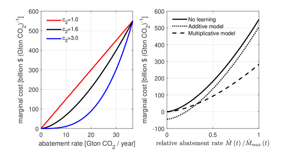
Figure 1: Marginal abatement cost curves with different exponents and the effects of additive and multiplicative models of endogenous learning for $c_{2}=1.6$.

The optimal abatement rate grows with time due to combined effects of economic growth and the interest rate. Taking income elasticity of global CO₂ emissions as $\theta=0.75$ , emissions intensity under BAU evolves as $\frac{d\mu}{dt}\cong-\left(1-\theta\right)r\mu$ and, with $r=4$%, this becomes $\frac{d\mu}{dt}\approx-0.01\mu$ , mimicking the rate of exogenous reduction in emissions intensity within DICE (Nordhaus and Sztorc (2013)). Then BAU emissions grow at $r_{BAU}\left(t\right)=0.75r\left(t\right)$, with the parameter $\dot{M}_{max}\left(t\right)$ also rising at this rate. For the simulations below, $r\left(t\right)$ decreases exponentially from the present value $r\left(0\right)=4$% with an e-folding time of $\tau_{r}=40$ years, so that $R\left(t\right)=\tau_{r}r\left(0\right)\left(1-e^{-t/\tau_{r}}\right)$ and $\dot{E}_{BAU}\left(t\right)=\dot{E}_{BAU}\left(0\right)e^{\theta\tau_{r}r\left(0\right)\left(1-e^{-t/\tau_{r}}\right)}$ so cumulative emissions under BAU are estimated numerically.

5.2 Optimal abatement pathways and carbon tax growth rates

The optimal abatement rate in the absence of learning or damages grows as $\frac{1}{\dot{M}\left(t\right)}\frac{d\dot{M}\left(t\right)}{dt}=\frac{i\left(t\right)}{c_{2}}+\theta r\left(t\right)$, and is integrated for the abatement rate in Figure 2a. GDP growth leads to expansion of abatement possibilities and rise in the abatement rate with time, but this effect is decreasing with declining economic growth, as seen in the declining slope on the logarithmic scale. All the above effects are simply absorbed in evolution of the carbon tax, which increases at constant Hotelling’s rate $i$ in the absence of learning or damages (Eq. (20) and Figure 2d). Here the interest rate is assumed constant in time, however this restriction is not generally posed.

The main feature of the endogenous learning model, as noted earlier, is whether it appears through an additive or multiplicative term. Empirical studies indicate a multiplicative model, having power-law structure $h\left(M\right)=M^{-b}$, with $b>0$ (Rubin et al. (2004); Lindman and Soderholm (2012)), adapted here to $h\left(M\right)=\left(M\left(t\right)/M\left(t=0\right)\right)^{-b}$ with $M\left(t=0\right)>0$ in order that $h\left(0\right)=1$. This has constant relative reductions of marginal cost, by $\left(\frac{1}{2}\right)^{b}$, per doubling of cumulative abatement. We also try exponential model $h\left(M\right)=e^{-M/M_{h}}$, with $M\left(t=0\right)\ll M_{h}$ so that $h\left(0\right)\cong 1$, giving rise to proportional reductions in marginal cost per unit increase in cumulative abatement, with constant $\partial\beta/\partial M=-\beta/M_{h}$. Such a choice depends on whether proportional cost reductions arise from doublings or unit increases of cumulative abatement. In both cases, the multiplicative model of learning has delayed abatement, compared to the no-learning case, with initially lower abatement rates later exceeding the no-learning case (Figure 2a). The exponential and power-law models do differ in important ways, with the latter’s influence declining with time, whereas the exponential model makes a growing difference with time. The power-law model depends on doublings of cumulative abatement, which become infrequent with time, whereas the exponential model depends on constant changes in cumulative abatement which occur more rapidly as abatement proceeds.

Emissions (Figure 2b) for these scenarios display the aforementioned discontinuity at the start of abatement. Global warming (Figure 2c) shows, for the more stringent abatement case, overshoot of global warming owing to the requirement of negative emissions for meeting the cumulative abatement goal. The overshoot is larger with the exponential learning model, owing to slower abatement early on. The carbon tax (Figure 2d) grows more slowly with learning, as shown earlier, with its magnitude being initially lower compared to the no-learning case for these multiplicative models, because initial abatement rates are reduced in this case, giving rise to smaller carbon taxes throughout. The exponential model has learning progressing rapidly, and thus for the stringent mitigation cases the departure from Hotelling’s rule is greater because the relative effect of learning on the growth rate is, from Eq. (20), $-\left(c_{2}+1\right)\frac{\dot{M}\left(t\right)}{i\left(t\right)M_{h}}$, whose magnitude increases with the abatement rate.

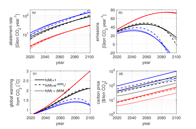
Figure 2: Effects of learning models with a multiplicative term: (a): Optimal abatement rates solving Eq. (14); (b): Emissions of CO₂; (c) Global warming contribution of CO₂; (d) Evolution of global carbon tax. The interest rate is $i=0.03$. Red, black and blue curves correspond to cumulative abatement goals of $M_{tot}=1000$ ,$M_{tot}=3000$, and $M_{tot}=5000$ Gton CO₂ respectively. The carbon tax grows at the rate of approximately $0.03$ per year in the no-learning case as expected from Eq. (20), with estimated $95$-percent confidence interval of $\left[0.0297,0.0298\right]$ for the mean growth rate in numerical calculations. For the exponential model, the corresponding $95$-percent confidence intervals are $\left[0.0281,0.0283\right]$, $\left[0.0249,0.0256\right]$, and $\left[0.0219,0.0231\right]$ for $M_{tot}$ of $1000$, $3000$, and $5000$ Gton respectively. For the power-law model these are the same $\left[0.0263,0.0267\right]$ for all the different values of $M_{tot}$.

An additive model of learning, such as $f\left(M\right)=c_{f}M$, has higher abatement rate early on compared to the no-learning case (Figure 3a). Overshoot is marginally lower in the stringent abatement case (Figure 3c), owing to lower emissions early on (Figure 3b). This comes from higher carbon taxes early on (Figure 3d), which become lower than the no-learning case only much later. Generally, additive models of learning lead to higher average carbon taxes than multiplicative models of learning. Since learning is proportional to cumulative abatement, the largest departures from Hotelling’s rule occur for the less stringent abatement scenarios, because from Eq. (20) its relative effect is $-\frac{c_{f}}{i\left(t\right)\left\{\beta\left(M\left(t\right),\dot{M}\left(t\right)\right)/\dot{M}\left(t\right)\right\}}$ which is decreasing in $\dot{M}$ as the marginal cost curve is strictly convex.

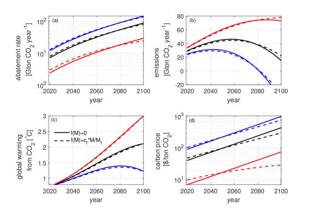
Figure 3: Effects of learning models with an additive term: (a): Optimal abatement rates solving Eq. (14); (b): Emissions of CO₂; (c) Global warming contribution of CO₂; (d) Evolution of global carbon tax. The interest rate is $i=0.03$. Red, black and blue curves correspond to cumulative abatement goals of $M_{tot}=1000$ ,$M_{tot}=3000$, and $M_{tot}=5000$ Gton CO₂ respectively. The carbon tax grows at the rate of approximately $0.03$ per year in the no-learning case as before. For the additive learning model shown here, the estimated $95$-percent confidence intervals of the mean growth rate are $\left[0.0130,0.0139\right]$, $\left[0.0226,0.0228\right]$, and $\left[0.0247,0.0248\right]$ for $M_{tot}$ of $1000$, $3000$, and $5000$ Gton respectively.

5.3 Effects of climate damage models

While typically, climate damages are treated as a function of global warming (Nordhaus (1993); Dietz and Venmans (2019)), for which there is considerable evidence (Burke et al. (2015)), and hence modeled as a function of cumulative abatement in our framework, in general one might also expect other influences. In particular, one might expect terms $\dot{M}\left(t\right)$, and $\int_{0}^{t}M\left(s\right)ds$ in conjunction with stochastic terms to play a role, to account for effects of rate of global warming, global sea-level rise whose rate of change also depends on the present global warming (Rahmstorf (2007); Vermeer and Rahmstorf (2009)), and lastly internal weather and climate variability. Despite its importance, optimization relative to the time-integral of $M\left(t\right)$ is not admitted by our present framework although such an extension is definitely possible, and hence we retain a model in $M\left(t\right)$ alone while noting its limitations, including the omission of slow and delayed effects of sea-level rise whose consideration can influence abatement pathways.

A model commonly adopted is the power-law function of global warming (e.g. Nordhaus and Sztorc (2013)), written here as $d\left(M\left(t\right)\right)=\frac{d_{0}}{T_{0}^{d_{1}}}\left\{\alpha\left(E_{BAU}\left(t\right)-M\left(t\right)\right)\right\}^{d_{1}}$ , for which damage fraction $d\left(t\right)$ grows $2^{d_{1}}$ for each doubling of warming $\triangle T$, which occur more frequently at smaller values (Figure 4). An alternative is logistic $d\left(M\left(t\right)\right)=\frac{1}{1+\frac{1}{d_{2}}e^{-\left(E_{BAU}\left(t\right)-M\left(t\right)\right)/E_{D}}}$, approximating the exponential for small $M\left(t\right)$, and $1$ for large values. Both models possess two free parameters, estimated from specifying a $5$% GDP damage fraction for $\Delta T=2.5$ K, growing to $20$% for $\Delta T=5$ K. Owing to this constraint, for $\Delta T$ of a few degrees, the two models are similar (Figure 4), but the inset shows that the power-law is more sensitive.

Including the minimization of damage costs leads to early abatement, compared to simulations that do not also include such costs, with higher initial abatement rates (Figure 5a) leading to somewhat delayed negative emissions (Figure 5b) and lowering of the overshoot in temperature (Figure 5c). The power-law model is more consequential, since the damages are more sensitive to temperature change, and this leads to higher starting carbon prices that grow at smaller rates compared to the simulations where damage costs are not counted. The effect is larger in scenarios with little abatement, because damage costs are greater.

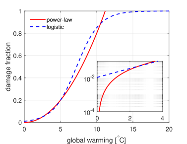
Figure 4: Power law and logistic models of the damage fraction as a function of global warming. For the range of global warming shown here, the logistic model can be approximated by the exponential as it follows a straight line on the logarithmic scale (inset). Damages in the power-law model grow more rapidly over the temperature range of interest.

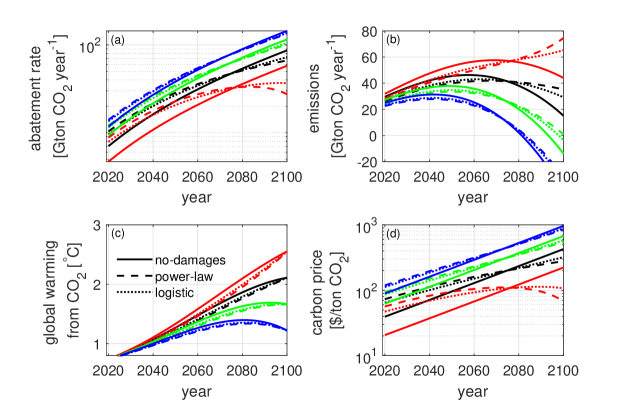
Figure 5: Effects of damage models: (a): Optimal abatement rates solving Eq. (14); (b): Emissions of CO₂; (c) Global warming contribution of CO₂; (d) Evolution of global carbon tax. The interest rate is $i=0.03$. Red, black, green and blue curves describe cumulative abatement goals of $M_{tot}=2000$ , $3000$, $4000$ and $5000$ Gton CO₂ respectively. The inclusion of damages leads to early abatement for the same cumulative constraint. The power-law model leads to somewhat larger abatement rates than the logistic model. Damages have a larger impact on the abatement pathway and carbon taxes for the less stringent abatement scenarios.

Multiplicative learning and damages have countervailing effects on the abatement rate, and their relative effects for the exponential and power-law models of learning and damages respectively are, from Eq. (14), equal to $\frac{c_{2}}{d_{1}}\frac{A\left(t\right)/M_{h}}{D\left(t\right)/E\left(t\right)}$, where $A\left(t\right)=\gamma\left(t\right)\dot{M}\left(t\right)$ is the annual abatement cost from Eq. (9) and $D\left(t\right)$ is damage cost. Damages are convex in global warming, and hence in cumulative emissions $E\left(t\right)$. This makes the ratio of damages per cumulative emissions in the denominator higher in scenarios with high cumulative emissions, for which corresponding abatement costs are lower. Thus we can expect the modeling of damage costs to play a greater role in scenarios with weak abatement, and contrariwise with stringent abatement. Similarly, while both learning and damages lower the carbon tax growth rate, their relative importance for this growth rate depends on the factor $\frac{1}{d_{1}}\frac{A\left(t\right)/M_{h}}{D\left(t\right)/E\left(t\right)}$. The carbon tax growth rate depends more strongly on the uncertain damage model in low-abatement scenarios, and on the learning model in high-abatement scenarios (Figure 6). The axes are damage fraction at $\triangle T=2.5$ K, fixing $d_{1}=2$, and learning parameter $M_{h}$, with small and large values, in the respective limiting cases, corresponding to learning and damages not being counted.

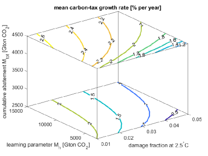
Figure 6: Contours of the carbon tax growth rate, (in percent per year) as a function of the damage fraction for global warming of 2.5 degrees C and the learning parameter of the exponential model, for two different cumulative abatement goals. The growth rate is always smaller than the interest rate, which is taken to be $0.03$ .

5.4 Initial carbon tax and cost of delaying abatement

We derived an expression for initial carbon tax in Eq. (27), assuming that learning and damages are not counted in the optimal pathway. This is graphed for constant GDP growth and interest rates, for abatement starting at the present year with $N=0$. Substituting from Eq. (30) the initial tax is

$$P\left(0\right)=c_{1}\left(c_{2}+1\right)\left\{\int_{0}^{T}e^{\theta R\left(t\right)}dt-\frac{\Delta T_{final}-\Delta T\left(0\right)}{\alpha\dot{M}_{max}\left(0\right)}\right\}\frac{1}{\left\{\int_{0}^{T}e^{I\left(t\right)/c_{2}+\theta R\left(t\right)}dt\right\}^{c_{2}}}$$ (34)

where $\triangle T_{final}$ is global warming from preindustrial times at the end of the time-horizon and $\Delta T\left(0\right)$ is the present global warming from past cumulative emissions of CO₂. Contour plots (Figure 7) show that, in addition to rapid GDP growth and more stringent goals involving smaller $\Delta T_{final}$, the initial tax is very sensitive to the interest rate. Low interest rates give rise to larger abatement rates early on (compared to high interest rates) in the optimal pathways, which must correspond to a higher initial carbon tax.

Figure 7: Initial value of the carbon tax ($ / ton CO₂), assuming that abatement begins at the present, i.e. $N=0$. The carbon tax is shown as contours of GDP growth rate and the total global warming from CO₂ $\Delta T_{final}$, for different values of risk-free interest rate in each panel. Calculations assume mean TCRE, of $1.65$ K / Tton C. The initial carbon tax is higher for lower interest rates, high rates of GDP growth, and stringent abatement goals.

An abatement delay by one year, postponing the onset of a carbon tax, increases the required initial value of the tax. The relative increase, shown in Eq. (28), has two contributions: the annual growth rate of the carbon tax by the Hotelling rule, and a second term describing the increasing average costs of abatement borne due to the higher abatement rates necessary for meeting the cumulative abatement goal. The second contribution grows identically as the present value of abatement cost for each year of delay, as comparison of Eqs. (24) and (28) showed. The reason is straightforward: the present value (at $t=0$) of the average carbon tax (between years $t=N$ and $t=T)$ grows at this rate, for each year of delay, and with average cost of mitigation being proportional to the marginal cost, the present value of the abatement cost also grows at this rate.

This growth rate, from Eq. (24), is graphed versus the year of starting abatement $N$ (Figure 8), for different GDP growth rates and interest rates. Its value increases for each year of delay, approaching $c_{2}$ as $N$ approaches $T$. Lower interest rates, by inducing higher rates of abatement early on, increasing the costs of delaying abatement by one year. Higher GDP growth rates give rise to larger growth in abatement rates with time, as abatement options grow with BAU emissions. Hence rapid economic growth has the effect of lowering the costs of delaying abatement, in relative terms.

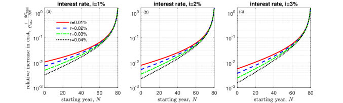
Figure 8: Growth rate of the present value of cost of delaying abatement by one year, in Eq. (24), for different starting years $N$, GDP growth rates, and interest rates. Growth rate is larger for lower interest rate and GDP growth rates, and increases rapidly for each year of delay.

5.5 Minimum global warming without overshoot

Our optimal pathways in Eq. (14) do not specify the avoidance of temperature overshoot, but this distinction is important. Therefore we examined the threshold (i.e. minimum) global warming goal that can be met without overshoot, in Eq. (33), based on the requirement of net positive emissions throughout, i.e. $\sigma\left(t\right)<1$ for all $t<T$, and reaching zero emissions only at $t=T$. Figure 9 shows the resulting threshold (i.e. minimum) CO₂-induced global warming attainable in 2100, given the history of CO₂ emissions and mean TCRE, and through the optimal abatement pathways modeled here. The starting year of abatement and the interest rate are important constraints, in addition to GDP growth, because large increases in abatement rate would pose increased abatement costs in the future. As a result, if the start of abatement is considerably delayed, options for substantially limiting CO₂-induced global warming become increasingly costly. Each year of delay leads to an increase in the threshold global warming by an increasing amount, because the abatement rate grows at a positive rate given by $\frac{i}{c_{2}}+\theta r$.

Since optimal pathways can abate only a fraction of future BAU emissions, rapid economic growth leads to an increase in the threshold. For example for long time-horizons with an early start to abatement, roughly $\theta r/\left(\frac{i}{c_{2}}+\theta r\right)$ of BAU emissions is abated by the optimal pathway. Larger interest rates lower the fraction of BAU emissions abated, because they lead to smaller abatement rates early on, thereby raising the temperature threshold. For example, with an interest rate of $3$ % it does not appear possible to meet a $1.5$ K global warming goal, even at mean TCRE, let alone the higher estimates, unless future GDP growth were to be practically negligible. In contrast if interest rates are closer to $1$ %, then in principle the more stringent global warming goals can be met even with rapid GDP growth, but this corresponds to a high carbon tax early on.

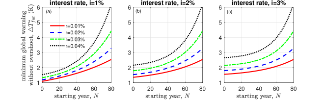
Figure 9: The minimum CO₂-induced warming threshold in 2100, for mean TCRE, in optimizing scenarios without overshoot. This threshold is lower in case of slower GDP growth and early start to abatement with smaller $N$. It is also lower in case of smaller risk-free interest rates. The threshold rises by an increasing amount for each year of delay in starting abatement, because the optimal abatement rate grows with time.

6 Conclusions and discussion

Global warming from CO₂ is roughly proportional to cumulative emissions, and more generally independent of emissions pathway (Herrington and Zickfeld (2014); Seshadri (2017a)), and such “path-independence” gives rise to cumulative emissions accounting and the concept of carbon budgets (Stocker (2013); Matthews et al. (2018)), presenting a simplification robust to climate modeling uncertainty. It also poses new questions about economic analyses of climate change abatement, through reducing CO₂ emissions, under an exogenous constraint on cumulative emissions.

Unlike a Pigouvian tax, one that internalizes the estimated future damage costs of emitting activities (Pearce (2003); Pindyck (2019)), by approximating the social cost of carbon (SCC) (Appendix 7), the present approach takes the carbon tax value to be instrumental in achieving stringent emissions goals (Rogelj et al. (2011, 2015); Millar et al. (2017)). These, as well as the Paris Agreement (UNFCCC (2015)), the context for discussion of global warming mitigation, do not make direct appeal to estimates of the SCC (Meinshausen et al. (2009); Hoegh-Guldberg et al. (2018)), which is notoriously difficult to estimate, although it is recognized that the SCC is quite large and has been underestimated in the past (see for e.g. Hope (2006); Nordhaus (2017); Ricke et al. (2018); Pindyck (2019)). Moreover, carbon taxes in the present approach are more straightforward to calculate, as the discussion surrounding Eqs. (20) and (65) shows; the SCC requires computing discounted future effects of a CO₂ pulse and variation with time (Appendix 7), whereas in the present approach the challenge of integrating climate models is averted by the finding that global warming at time $t$ only depends on cumulative emissions until then. However, a price must be paid: the carbon tax can be higher or lower than the SCC, since the present approach doesn’t restrain its economic efficiency. For example, imagine a rapid increase in temperature or the damage function that would portend rapid increase in the SCC around future time $t^{*}$: the former approach would have carbon tax increasing rapidly around $t^{*}$, whereas that based on a cumulative emissions constraint has it growing roughly at the interest-rate.

Such an approach requires simple models of abatement, and we have developed a model based on an increasing marginal abatement cost curve that is shifted down or scaled in the presence of endogenous learning, through either an additive or multiplicative term or both. The model is similar to that of Emmerling et al. (2019), with explicit treatment of the effects of economic growth and furthermore endogenous learning on the abatement curve. As the economy grows, business as usual emissions grow correspondingly, and this leads to expansion of abatement options and horizontal stretching of the cost curve. The present work has many points of commonality with previous studies examining economics under a cumulative abatement constraint (Dietz and Venmans (2019); Emmerling et al. (2019); van der Ploeg and Rezai (2019)), but there are new features in the treatment of endogenous learning in addition to climate damages, and analysis for time-varying rates, in addition to applications to problems relevant to abatement. The main findings are summarized below:

Optimal growth rates of abatement and the carbon tax

• When learning and damages are not counted, the abatement rate relative to the maximum abatement rate, which we denoted as $\sigma\left(t\right)$, has growth rate given by the ratio of the risk-free interest rate and the exponent of the abatement cost curve. A higher exponent, i.e. sharply rising, abatement cost curve makes the abatement rate grow more slowly, limiting future rise in abatement costs. This is consistent with previous studies, e.g. Emmerling et al. (2019).

• However, the carbon tax growth rate equation is unaffected by the shape of the marginal abatement cost curve, following Hotelling’s rule, similarly to previous studies (Dietz and Venmans (2019); Emmerling et al. (2019)). A sharply rising abatement cost curve gives rise to a higher initial abatement rate for the same carbon tax, with the abatement rate growing more slowly with time.

Effects of climate damage costs and endogenous learning

• If cost-minimization accounts for endogenous learning, the carbon price grows at a smaller rate as future marginal costs are reduced.

• Damage costs affect the optimal abatement pathway, especially where the goal specifies less stringent levels of cumulative abatement, for which global warming and resulting damage costs are higher. Limiting damage costs, in addition to abatement costs, requires a higher carbon price early on and therefore the subsequent growth rate of the carbon tax can be smaller.

• The effect of endogenous learning on the initial carbon tax depends on whether it enters as an additive of multiplicative model, i.e. whether it shifts the marginal abatement cost curve down or reduces it by a constant factor. Additive learning models lead to higher initial abatement rates, in turn requiring a higher initial carbon tax. Multiplicative learning models lead to slow abatement initially, involving lower starting carbon taxes.

• Additive models of learning influence the optimal abatement rate only if the interest rate is non-zero, owing to increasing marginal costs (Appendix 5). However they reduce the growth rate of the carbon tax regardless, because benefits of cost reductions do not depend on the interest rate.

• Empirical literature on learning curves generally points to a multiplicative model, implying lower initial carbon taxes (compared to the no-learning case) that grow at a smaller rate. Competition between multiplicative learning and damage effects on the abatement rate is resolved according to the stringency of the abatement scenario: higher dependence on learning in high-abatement scenarios, and on damages in low-abatement scenarios.

Initial carbon tax and cost of delaying abatement

• The initial carbon tax rises with the stringency of abatement and the BAU emissions, and is larger for lower interest rates as these lead to higher abatement rates early on. The importance of a low discount rate for the stringency of early abatement was emphasized previously by Emmerling et al. (2019).

• Delaying the start of abatement is costly as we have assumed that the marginal abatement cost curve is increasing with the abatement rate. Each year of delay leads to an increase in the total cost of abatement in present value terms at $t=0$. A positive interest rate does not imply that abatement can be costlessly postponed in a cumulative emissions framework, because this has been factored into the optimal abatement pathways. As a result, the need for more rapid abatement drives the cost of a delay.

• The growth rate of the present value cost is larger for lower interest rate and GDP growth rates, and increases rapidly for each year of delay. Lower interest rates induce higher abatement rates early on and therefore lead to higher relative costs of delaying abatement. Slower GDP growth leads to a smaller growth in future abatement, so the relative costs of delaying abatement are high.

• The relative increase in the cost of delay by one year does not depend on the abatement level, but increases rapidly with proximity to the end of the time-horizon.

• Each year of delay in abatement, postponing a global carbon tax, requires a corresponding increase in the initial value of the tax if abatement begins the following year. The carbon tax growth rate for each year of delay has two components: a Hotelling rate, and a contribution identical to the growth rate in present value expenditures, because the marginal cost of abatement is proportional to the average cost when we assume that the abatement curve has zero intercept.

Economics of avoiding temperature overshoot

• Avoiding temperature overshoot is important for preventing climate change commitments that are irreversible, such as loss of ice-sheets and biodiversity. Owing to proportionality between global warming and cumulative emissions, overshoot in CO₂’s contribution to global warming generally corresponds to net negative emissions. Therefore, we estimated the global warming goal attainable without overshoot, $\triangle T_{fut}^{*}$, via optimizing pathways having net positive emissions throughout and reaching zero emissions only at $t=T$.

• This constraint of no net-negative emissions limits the threshold (i.e. minimum) $\triangle T_{fut}^{*}$. This threshold rises with GDP growth and a delayed start to abatement, because optimal pathways have the annual abatement rate growing at rates governed by the interest rate and economic growth. Hence they can abate only a fraction of future BAU emissions, and high cumulative emissions goals over short time-horizons cannot be met without net negative emissions.

• The threshold is reduced for smaller risk-free interest rates, and high growth of the abatement cost, because these give rise to higher abatement rates early on. For long time-horizons assuming an early start to abatement, roughly the fraction $\theta r/\left(\frac{i}{c_{2}}+\theta r\right)$ of BAU emissions is abated. Only in the limit of zero interest rates can all of BAU emissions be abated by stringent optimizing trajectories.

• Each year of delay in starting abatement makes the threshold larger by an increasing amount, with marginal effects measured as $\partial\triangle T_{fut}^{*}/\partial N$, rising as long as the optimal pathway has annual abatement rate growing.

• Overshoot increases by a small amount when effects of (multiplicative) learning are included, and decreases by a small amount when economic costs of climate damages are counted in the optimization. This effect might increase if the damage fraction considers delayed effects, but this has not been modeled.

Creating yet more optimization-based models of abatement without constraint from conservation principles or economic data is risk prone, especially in studying long-term futures. At the same time, cumulative emissions budgets pose an important constraint on global warming abatement, whose implications for economic optimization approaches are an important research area, leading to a growing body of work (Dietz and Venmans (2019); Emmerling et al. (2019)). This paper has sought to develop a simplified model to study the satisfaction of a cumulative emissions constraint at the lowest cost and, although the resulting thought experiment is quite rudimentary, there are some points of agreement with prior studies as noted above. There are also several simplifications, which future work could remedy, especially: making detailed estimates from data on costs, learning and damages, with effects of the integral of cumulative abatement also included to account for delayed effects such as those of sea-level rise; allowing for epistemic uncertainty in future economic growth and interest rates; and invoking further intertemporal choice criteria in studying decarbonization pathways.

Appendix 1: Emissions intensity under business as usual

Emissions intensity under business as usual at $t+\triangle t$ can be written as $\frac{\dot{E}_{BAU}+\triangle\dot{E}_{BAU}}{G+\triangle G}=\frac{1+\theta\frac{\triangle G}{G}}{1+\frac{\triangle G}{G}}\mu$, and expanding the denominator as its Taylor series

$$\frac{\dot{E}_{BAU}+\triangle\dot{E}_{BAU}}{G+\triangle G}=\left\{1+\left(\theta-1\right)\left(\left(\frac{\triangle G}{G}\right)-\left(\frac{\triangle G}{G}\right)^{2}+\ldots\right)\right\}\mu$$ (35)

The change is $\triangle\mu=\mu\left(t+\Delta t\right)-\mu\left(t\right)$, and considering the natural increment of $\triangle t=1$ year so that $\Delta G/G\equiv r$, the growth rate of global GDP, we obtain approximately

$$\frac{d\mu}{dt}\cong\frac{\triangle\mu}{\triangle t}=-\left(1-\theta\right)\left(r-r^{2}+r^{3}-\ldots\right)\mu$$ (36)

We might simplify the expression using the fact $r-r^{2}+r^{3}-\ldots$ is an infinite geometric series equaling $r/\left(1+r\right)$, so the evolution of emissions intensity under BAU is $\frac{d\mu}{dt}\cong-\left(1-\theta\right)\frac{r}{1+r}\mu$.

Appendix 2: Derivation of Euler-Lagrange equation

For fixed $T$, in order to minimize the integral $\int_{0}^{T}g\left(t,M\left(t\right),\dot{M}\left(t\right)\right)dt$ subject to constraint $\int_{0}^{T}m\left(t\right)dt=M_{tot}$, we first define $I\left(M\left(t\right),\dot{M}\left(t\right)\right)=\int_{0}^{T}g\left(t\right)dt+\lambda\left(\int_{0}^{T}\dot{M}\left(t\right)dt-M_{tot}\right)$. Stationary requires the first-variation $\delta I$ in the integral due to small changes $\delta M$ and $\delta\dot{M}$ to vanish. The variation $\delta I=I\left(M+\delta M,\dot{M}+\delta\dot{M}\right)-I\left(M,\dot{M}\right)$ is

$$\delta I=\int_{0}^{T}\left\{\frac{\partial g}{\partial M}\delta M+\frac{\partial g}{\partial\dot{M}}\delta\dot{M}+\lambda\left(\frac{\partial\dot{M}}{\partial M}\delta M+\frac{\partial\dot{M}}{\partial\dot{M}}\delta\dot{M}\right)\right\}dt=0$$ (37)

and, integrating by parts, $\int_{0}^{T}\frac{\partial g}{\partial\dot{M}}\delta\dot{M}dt=-\int_{0}^{T}\frac{d}{dt}\left(\frac{\partial g}{\partial\dot{M}}\right)\delta Mdt$ after applying the condition that $\delta M\left(0\right)=\delta M\left(T\right)=0$ because the variations must preserve boundary conditions of the problem. There is a corresponding equation involving the integral constraint on cumulative negative emissions. Combining these equations yields

$$\delta I=\int_{0}^{T}\left\{\frac{\partial g}{\partial M}-\frac{d}{dt}\left(\frac{\partial g}{\partial\dot{M}}\right)+\lambda\left(\frac{\partial\dot{M}}{\partial M}-\frac{d}{dt}\left(\frac{\partial\dot{M}}{\partial\dot{M}}\right)\right)\right\}\delta Mdt=0$$ (38)

for arbitrary changes $\delta M$, yielding the Euler-Lagrange Eq. (12).

Appendix 3: Terms in Euler-Lagrange equation

From Eqs. (11) and (13)

$$\frac{\partial g}{\partial M}=-e^{-I\left(t\right)}f^{\prime}\left(M\left(t\right)\right)h\left(M\left(t\right)\right)\dot{M}\left(t\right)+e^{-I\left(t\right)}\left\{c_{0}+c_{1}\left(\frac{\dot{M}\left(t\right)}{\dot{M}_{max}\left(t\right)}\right)^{c_{2}}-f\left(M\left(t\right)\right)\right\}h^{\prime}\left(M\left(t\right)\right)\dot{M}\left(t\right)\\ +e^{-I\left(t\right)}d^{\prime}\left(M\left(t\right)\right)G\left(t\right)$$ (39)

whereas

$$\frac{\partial g}{\partial\dot{M}}=e^{-I\left(t\right)}c_{1}c_{2}\left(\frac{\dot{M}\left(t\right)}{\dot{M}_{max}}\right)^{c_{2}}h\left(M\left(t\right)\right)+e^{-I\left(t\right)}\left\{c_{0}+c_{1}\left(\frac{\dot{M}\left(t\right)}{\dot{M}_{max}\left(t\right)}\right)^{c_{2}}-f\left(M\left(t\right)\right)\right\}h\left(M\left(t\right)\right)$$ (40)

Here we have assumed that $\dot{M}_{max}\left(t\right)$ is a known function of time, which can be related to BAU emissions, and hence independent of $M\left(t\right)$ and $\dot{M}\left(t\right)$. The above equation simplifies to

$$\frac{\partial g}{\partial\dot{M}}=e^{-I\left(t\right)}\left\{c_{0}+c_{1}\left(c_{2}+1\right)\left(\frac{\dot{M}\left(t\right)}{\dot{M}_{max}\left(t\right)}\right)^{c_{2}}-f\left(M\left(t\right)\right)\right\}h\left(M\left(t\right)\right)$$ (41)

so that

$$\frac{d}{dt}\left(\frac{\partial g}{\partial\dot{M}}\right)=-i\left(t\right)e^{-I\left(t\right)}\left\{c_{0}+c_{1}\left(c_{2}+1\right)\left(\frac{\dot{M}\left(t\right)}{\dot{M}_{max}\left(t\right)}\right)^{c_{2}}-f\left(M\left(t\right)\right)\right\}h\left(M\left(t\right)\right)\\ +e^{-I\left(t\right)}\left\{\frac{c_{1}c_{2}\left(c_{2}+1\right)}{\dot{M}_{max}^{c_{2}}}\dot{M}\left(t\right)^{c_{2}-1}\ddot{M}\left(t\right)-f^{\prime}\left(M\left(t\right)\right)\dot{M}\left(t\right)\right\}h\left(M\left(t\right)\right)\\ +e^{-I\left(t\right)}\left\{c_{0}+c_{1}\left(c_{2}+1\right)\left(\frac{\dot{M}\left(t\right)}{\dot{M}_{max}\left(t\right)}\right)^{c_{2}}-f\left(M\left(t\right)\right)\right\}h^{\prime}\left(M\left(t\right)\right)\dot{M}\left(t\right)\\ -e^{-I\left(t\right)}c_{1}c_{2}\left(c_{2}+1\right)\left(\frac{\dot{M}\left(t\right)}{\dot{M}_{max}\left(t\right)}\right)^{c_{2}}\frac{1}{\dot{M}_{max}\left(t\right)}\left\{\frac{d}{dt}\dot{M}_{max}\left(t\right)\right\}h\left(M\left(t\right)\right)$$ (42)

Using $\frac{\partial\dot{M}}{\partial M}=0$ and $\frac{\partial\dot{M}}{\partial\dot{M}}=1$, so that $\frac{d}{dt}\left(\frac{\partial\dot{M}}{\partial\dot{M}}\right)=0$ we finally obtain

$$d^{\prime}\left(M\left(t\right)\right)G\left(t\right)=-i\left(t\right)\left\{c_{0}+c_{1}\left(c_{2}+1\right)\left(\frac{\dot{M}\left(t\right)}{\dot{M}_{max}}\right)^{c_{2}}-f\left(M\left(t\right)\right)\right\}h\left(M\left(t\right)\right)\\ +\frac{c_{1}c_{2}\left(c_{2}+1\right)}{\dot{M}_{max}^{c_{2}}}\dot{M}\left(t\right)^{c_{2}-1}\ddot{M}\left(t\right)h\left(M\left(t\right)\right)+\frac{c_{1}c_{2}}{\dot{M}_{max}^{c_{2}}}\dot{M}\left(t\right)^{c_{2}+1}h^{\prime}\left(M\left(t\right)\right)\\ -c_{1}c_{2}\left(c_{2}+1\right)\left(\frac{\dot{M}\left(t\right)}{\dot{M}_{max}\left(t\right)}\right)^{c_{2}}\frac{1}{\dot{M}_{max}\left(t\right)}\left\{\frac{d}{dt}\dot{M}_{max}\left(t\right)\right\}h\left(M\left(t\right)\right)$$ (43)

and taking the 2^nd derivative term to one side and dividing by $h\left(t\right)>0$ yields Eq. (14).

Appendix 4: Effects on marginal cost curve of the learning models

Let us consider the influence of the two models of endogenous learning on the marginal cost curve. Average cost $\gamma\left(\dot{M},M\right)$ is related to marginal cost $\beta\left(M,\dot{M}\right)$ as $\gamma\left(M,\dot{M}\right)=\frac{1}{\dot{M}}\int_{0}^{\dot{M}}\beta\left(M,\dot{s}\right)d\dot{s}$ where $\dot{s}$ is integrated from $0$ to $\dot{M}$ . Substituting for the form of the average cost in Eq. (3), marginal cost is related as

$$\int_{0}^{\dot{M}}\beta\left(M,\dot{s}\right)d\dot{s}=\left(c_{0}+c_{1}\left(\frac{\dot{M}\left(t\right)}{\dot{M}_{max}}\right)^{c_{2}}-f\left(M\right)\right)h\left(M\right)\dot{M}$$ (44)

and differentiating with respect to $\dot{M}$

$$\beta\left(M,\dot{M}\right)=\left\{c_{0}+\frac{\left(c_{2}+1\right)c_{1}}{\dot{M}_{max}^{c_{2}}}\dot{M}^{c_{2}}-f\left(M\right)\right\}h\left(M\right)$$ (45)

which makes it clear that $f\left(M\right)$ is an additive contribution to the marginal cost curve whereas $h\left(M\right)$ multiplies it throughout.

Appendix 5: Effect of additive endogenous learning with zero interest rate

The need for nonzero interest rate $i\left(t\right)$, for a non-zero effect of the additive learning model on the optimal abatement pathway, arises even if we assume that there is no GDP growth, wherein $r_{BAU}\left(t\right)=0$ and $\dot{M}_{max}$ is constant. Therefore we make these restrictions in our discussion of origins of this behavior. Consider abatement rate $\dot{M}\left(t\right)=\frac{M_{tot}}{T}+\epsilon x\left(t\right)$, with $0<\epsilon\ll\frac{M_{tot}}{T}$, so that $\epsilon x\left(t\right)$ is a small perturbation to a trajectory with constant abatement rate. Cumulative abatement rate in this case is $M\left(t\right)=\int_{0}^{t}\dot{M}\left(s\right)ds=M_{tot}\frac{t}{T}+\epsilon X\left(t\right)$, where $X\left(t\right)=\int_{0}^{t}x\left(s\right)ds$. Boundary conditions on $M\left(t\right)$ require $X\left(0\right)=X\left(T\right)=0$. If only the additive model is $f\left(M\left(t\right)\right)$ is active, with $h\left(M\left(t\right)\right)$ being fixed at $1$, the abatement cost in year $t$ is, from Eq. (9), after substituting the models of $M\left(t\right)$ and $\dot{M}\left(t\right)$ above

$$A\left(t\right)=c_{0}\left\{\frac{M_{tot}}{T}+\epsilon x\left(t\right)\right\}+\frac{c_{1}}{\dot{M}_{max}}\left(\frac{M_{tot}}{T}+\epsilon x\left(t\right)\right)^{c_{2}+1}\\ -\left\{\frac{M_{tot}}{T}+\epsilon x\left(t\right)\right\}f\left(M_{tot}\frac{t}{T}+\epsilon X\left(t\right)\right)$$ (46)

We have assumed that $\dot{M}_{max}$ is constant, as in a steady-state GDP trajectory, as this simplifies our discussion. As noted above, the effect of the interest rate on additive learning does not depend on any growth assumptions. We furthermore approximate the function $f$ above by its Taylor series truncated to $1$^st-order and following some algebra, and counting only abatement costs, the discounted expenditure in case $i=0$ simplifies to

$$C_{total}=\int_{0}^{T}A\left(t\right)dt=C_{0}M_{tot}-\frac{M_{tot}}{T}\int_{0}^{T}f\left(M_{tot}\frac{t}{T}\right)dt+\frac{c_{1}}{\dot{M}_{max}}\int_{0}^{T}\dot{M}\left(t\right)^{c_{2}+1}dt$$ (47)

as described below. Those uninterested in the details might skip the aside below to the discussion following Eq. (52), where the thread of the present discussion is resumed.

{Aside: In the following we derive Eq. (47). For abatement expenditure in year $t$ in Eq. (46), upon substituting the Taylor series expansion to $1$^storder in small parameter $\epsilon$

$$f\left(M_{tot}\frac{t}{T}+\epsilon X\left(t\right)\right)\cong f\left(M_{tot}\frac{t}{T}\right)+\epsilon X\left(t\right)f^{\prime}\left(M_{tot}\frac{t}{T}\right)$$ (48)

we obtain

$$A\left(t\right)=\frac{M_{tot}}{T}\left\{c_{0}-f\left(M_{tot}\frac{t}{T}\right)\right\}+\epsilon\frac{d}{dt}\left\{c_{0}X\left(t\right)-f\left(M_{tot}\frac{t}{T}\right)X\left(t\right)\right\}\\ +\frac{c_{1}}{\dot{M}_{max}}\left(\frac{M_{tot}}{T}+\epsilon x\left(t\right)\right)^{c_{2}+1}$$ (49)

where, for consistency, we have retained only $1$^st order terms in $\epsilon$ for the series-derived contributions. Total expenditure becomes, for $\delta=0$

$$C_{total}=\int_{0}^{T}\frac{M_{tot}}{T}\left\{c_{0}-f\left(M_{tot}\frac{t}{T}\right)\right\}dt+\\ \epsilon\int_{0}^{T}\frac{d}{dt}\left\{c_{0}X\left(t\right)-f\left(M_{tot}\frac{t}{T}\right)X\left(t\right)\right\}dt+\frac{c_{1}}{\dot{M}_{max}}\int_{0}^{T}\left(\frac{M_{tot}}{T}+\epsilon x\left(t\right)\right)^{c_{2}+1}dt$$ (50)

and, using

$$\int_{0}^{T}\frac{d}{dt}\left\{c_{0}X\left(t\right)-f\left(M_{tot}\frac{t}{T}\right)X\left(t\right)\right\}dt=\\ c_{0}\left(X(T)-X\left(0\right)\right)+f\left(T_{tot}\right)X\left(T\right)-f\left(0\right)X\left(0\right)=0$$ (51)

with the last equality following from boundary conditions on $X\left(t\right)$, we obtain

$$C_{total}=\int_{0}^{T}\frac{M_{tot}}{T}\left\{c_{0}-f\left(M_{tot}\frac{t}{T}\right)\right\}dt+\frac{c_{1}}{\dot{M}_{max}}\int_{0}^{T}\left(\frac{M_{tot}}{T}+\epsilon x\left(t\right)\right)^{c_{2}+1}dt$$ (52)

which simplifies to Eq. (47).}

It has been shown in the Aside that the $1$^st-order effect of an arbitrary additive learning function on a constant emissions trajectory is zero. Moreover, the effect of non-constant abatement rate enters only through the last term in Eq. (47), which we expect to be minimized by the constant abatement rate pathway. This is shown in the following. Since $c_{2}>0$, $p\left(\dot{M}\right)\equiv\dot{M}^{c_{2}+1}$ is a convex function of $\dot{M}$. Recall that emissions rate $\dot{M}\left(t\right)=\frac{M_{tot}}{T}+\epsilon x\left(t\right)$, with its mean value $\mathbf{E}\dot{M}=\frac{1}{T}\int_{0}^{T}\dot{M}\left(t\right)dt=\frac{M_{tot}}{T}$ and, furthermore

$$\mathbf{E}p\left(\dot{M}\right)=\frac{1}{T}\int_{0}^{T}p\left(\dot{M}\left(t\right)\right)dt=\frac{1}{T}\int_{0}^{T}\dot{M}\left(t\right)^{c_{2}+1}dt$$ (53)

From Jensen’s inequality, for a convex function $p\left(\dot{M}\right)$, $\mathbf{E}p\left(\dot{M}\right)\geq p\left(\mathbf{E}\dot{M}\right)$. But $p\left(\mathbf{E}\dot{M}\right)=\left(\frac{M_{tot}}{T}\right)^{c_{2}+1}$. Hence

$$\frac{1}{T}\int_{0}^{T}\dot{M}\left(t\right)^{c_{2}+1}dt\geq\left(\frac{M_{tot}}{T}\right)^{c_{2}+1}$$ (54)

or equivalently

$$\frac{c_{1}}{\dot{M}_{max}}\int_{0}^{T}\left(\frac{M_{tot}}{T}+\epsilon x\left(t\right)\right)^{c_{2}+1}dt\geq\frac{c_{1}}{\dot{M}_{max}}\int_{-T}^{0}\left(\frac{M_{tot}}{T}\right)^{c_{2}+1}dt$$ (55)

with equality occurring at $\epsilon=0$. Minimum entails $\epsilon=0$, so that the additive endogenous learning model does not influence the optimal path if the risk-free interest rate is zero. This result appeals to convexity of function $\dot{N}\left(t\right)^{c_{2}+1}$, but this does not limit its generality because the function is surely convex if $c_{2}>0$, where marginal costs are increasing.

Appendix 6: Present value of abatement cost without endogenous learning

Assuming the absence of endogenous learning, the present value of the abatement cost is

$$C_{total}=c_{1}\int_{N}^{T}e^{-I\left(t\right)}\sigma\left(t\right)^{c_{2}+1}\dot{M}_{max}\left(t\right)dt$$ (56)

assuming $c_{0}=0$, and using Eqs. (2) and (15). For this situation, from Eq. (16) $\sigma\left(t\right)=\sigma\left(N\right)e^{\int_{N}^{t}\frac{i\left(s\right)}{c_{2}}ds}=\sigma\left(N\right)e^{-I\left(N\right)/c_{2}}e^{I\left(t\right)/c_{2}}$, where we recall that $I\left(t\right)=\int_{0}^{t}i\left(s\right)ds$. Similarly, $\dot{M}_{max}\left(t\right)=\dot{M}_{max}\left(N\right)e^{\int_{N}^{t}\theta r\left(s\right)ds}$ can also be written as $\dot{M}_{max}\left(t\right)=\dot{M}_{max}\left(N\right)e^{-\theta R\left(N\right)}e^{\theta R\left(t\right)}$, whereupon

$$C_{total}=c_{1}\sigma\left(N\right)^{c_{2}+1}\dot{M}_{max}\left(N\right)e^{-I\left(N\right)\left(1+\frac{1}{c_{2}}\right)}e^{-\theta R\left(N\right)}\int_{N}^{T}e^{I\left(t\right)/c_{2}+\theta R\left(t\right)}dt$$ (57)

or equivalently

$$C_{total}=C\left(N\right)e^{-I\left(N\right)\left(1+\frac{1}{c_{2}}\right)}e^{-\theta R\left(N\right)}\int_{N}^{T}e^{I\left(t\right)/c_{2}+\theta R\left(t\right)}dt$$ (58)

where

$$C\left(N\right)=c_{1}\sigma\left(N\right)^{c_{2}+1}\dot{M}_{max}\left(N\right)$$ (59)

is the abatement cost during the initial year $t=N$. Its value is estimated from the cumulative abatement constraint. The evolution of the abatement rate is $\dot{M}\left(t\right)=\dot{M}\left(N\right)e^{\int_{N}^{t}\left\{\frac{i\left(s\right)}{c_{2}}+\theta r\left(s\right)\right\}ds}$, so the cumulative abatement becomes

$$M_{tot}=\int_{N}^{T}\dot{M}\left(t\right)dt=\dot{M}\left(N\right)e^{-I\left(N\right)/c_{2}}e^{-\theta R\left(N\right)}\int_{N}^{T}e^{I\left(t\right)/c_{2}+\theta R\left(t\right)}dt$$ (60)

from which $\sigma\left(N\right)=\dot{M}\left(N\right)/\dot{M}_{max}\left(N\right)$ reduces to

$$\sigma\left(N\right)=\frac{M_{tot}}{\dot{M}_{max}\left(0\right)}\frac{e^{I\left(N\right)/c_{2}}}{\int_{N}^{T}e^{I\left(t\right)/c_{2}+\theta R\left(t\right)}dt}$$ (61)

where we have used $\dot{M}_{max}\left(N\right)=\dot{M}_{max}\left(0\right)e^{\theta R\left(N\right)}$. Substituting into Eq. (59)

$$C\left(N\right)=c_{1}\left(\frac{M_{tot}}{\dot{M}_{max}\left(0\right)}\right)^{c_{2}+1}\dot{M}_{max}\left(0\right)\frac{e^{I\left(N\right)\left(1+\frac{1}{c_{2}}\right)}e^{\theta R\left(N\right)}}{\left\{\int_{N}^{T}e^{I\left(t\right)/c_{2}+\theta R\left(t\right)}dt\right\}^{c_{2}+1}}$$ (62)

so that finally, from Eq. (58)

$$C_{total}=c_{1}\left(\frac{M_{tot}}{\dot{M}_{max}\left(0\right)}\right)^{c_{2}+1}\dot{M}_{max}\left(0\right)\frac{1}{\left\{\int_{N}^{T}e^{I\left(t\right)/c_{2}+\theta R\left(t\right)}dt\right\}^{c_{2}}}$$ (63)

Appendix 7: Social cost of carbon

The social cost of carbon (SCC) is usually defined as the discounted damage costs from a pulse emission of CO₂, conventionally one ton

$$SCC\left(t\right)=\int_{t}^{\infty}e^{-\tilde{I}\left(t\right)}d^{\prime}\left(T\left(s\right)\right)G\left(s\right)\triangle\widetilde{T}\left(s\right)ds$$ (64)

where the SCC is discounted at a rate $\tilde{i}\left(t\right)$ that in general is distinct from the risk-free interest rate. The SCC is calculated assuming that a unit pulse of CO₂ is emitted at time $t$, and depends on the subsequent global warming contribution from that pulse $\triangle\widetilde{T}\left(s\right)$, $s\geq t$, with $\triangle\widetilde{T}\left(s=t\right)=0$; and on the sensitivity of global climate damages to temperature changes $d^{\prime}\left(T\left(s\right)\right)G\left(s\right)$. For example, for a power-law model of damage fraction the social cost of carbon is

$$SCC\left(t\right)=\frac{d_{1}}{TCRE}\int_{t}^{\infty}e^{-\tilde{I}\left(t\right)}\frac{D\left(s\right)}{E\left(s\right)}\triangle\widetilde{T}\left(s\right)ds$$ (65)

where, we recall, TCRE is the constant ratio of global warming to cumulative emissions, $d_{1}>1$ is the exponent of the damage function, and $D\left(s\right)/E\left(s\right)$ is the damage costs per cumulative emissions. Since damages are a convex function of global warming, this ratio is increasing as long as global temperature is rising. This is the main factor behind increasing SCC with time. The contribution $\triangle\widetilde{T}\left(s\right)$ depends on the competition between the diminishing radiative forcing from a unit pulse of CO₂, owing the logarithmic radiative forcing relation with excess concentrations, and the decreasing ability of the oceans to take up excess heat and CO₂, as global warming proceeds. Generally $\triangle\widetilde{T}\left(s\right)$ is not merely $\triangle\widetilde{T}\left(s-t\right)$ , but actually $\triangle\widetilde{T}\left(s-t,\triangle T\left(s\right),CO_{2}\left(s\right)\right),$i.e. depending not only on the time elapsed since the emission of the pulse, but also global warming $\triangle T\left(s\right)$ in the absence of the pulse which affects its fate in the atmosphere, as well as excess carbon-dioxide in the atmosphere $CO_{2}\left(s\right)$ in the absence of the pulse which affects the radiative forcing contribution from the pulse (Seshadri (2017b)). Furthermore, the ratio $D\left(s\right)/E\left(s\right)$ appearing in the integral, for times $s\geq t$, requires not only present values of global warming and cumulative emissions, but also assumptions about future evolution of cumulative emissions so that damages can be calculated for all times $s\geq t$. Clearly, the information needs for estimating the SCC are onerous and corresponding uncertainties are large.

References

- Allen et al. (2009) Allen, M. R., D. J. Frame, C. Huntingford, C. D. Jones, J. A. Lowe, M. Meinshausen, and N. Meinshausen (2009), Warming caused by cumulative carbon emissions towards the trillionth tonne, Nature, 458, 1163–1166, doi:http://dx.doi.org/10.1038/nature08019.
- Allen et al. (2016) Allen, M. R., J. S. Fuglestvedt, K. P. Shine, A. Reisinger, R. T. Pierrehumbert, and P. M. Forster (2016), New use of global warming potentials to compare cumulative and short-lived climate pollutants, Nature Climate Change, 6, 773–777, doi:10.1038/NCLIMATE2998.
- Arrow (1962) Arrow, K. J. (1962), The economic implications of learning by doing, The Review of Economic Studies, 29, 155–173, doi:10.2307/2295952.
- Bowerman et al. (2011) Bowerman, N. H. A., D. J. Frame, C. Huntingford, J. A. Lowe, and M. R. Allen (2011), Cumulative carbon emissions, emissions floors and short-term rates of warming: implications for policy, Philosophical Transactions of the Royal Society of London A, 369, 45–66, doi:http://dx.doi.org/10.1098/rsta.2010.0288.
- Burke et al. (2015) Burke, M., S. M. Hsiang, and E. Miguel (2015), Global non-linear effect of temperature on economic production, Nature, 527, 235–239, doi:10.1038/nature15725.
- Dietz and Venmans (2019) Dietz, S., and F. Venmans (2019), Cumulative carbon emissions and economic policy: In search of general principles, Journal of Environmental Economics and Management, 96(108-129), 108–129.
- Emmerling et al. (2019) Emmerling, J., L. Drouet, K.-I. van der Wijst, D. van Vuuren, V. Bosetti, and M. Tavoni (2019), The role of the discount rate for emission pathways and negative emissions, Environmental Research Letters, 14, 1–11, doi:10.1088/1748-9326/ab3cc9.
- Fraser (1992) Fraser, C. G. (1992), Isoperimetric problems in the variational calculus of Euler and Lagrange, Historia Mathematica, 19, 4–23, doi:10.1016/0315-0860(92)90052-d.
- Gillingham et al. (2008) Gillingham, K., R. G. Newell, and W. A. Pizer (2008), Modeling endogenous technological change for climate policy analysis, Energy Economics, 30, 2734–2753, doi:10.1016/j.eneco.2008.03.001.
- Goulder and Mathai (2000) Goulder, L. H., and K. Mathai (2000), Optimal CO2 Abatement in the Presence of Induced Technological Change, Journal of Environmental Economics and Management, 39, 1–38, doi:10.1006/jeem.1999.1089.
- Grubb (1993) Grubb, M. (1993), The costs of limiting fossil-fuel CO2 emissions: a survey and analysis, Annual Review of Energy and the Environment, 18, 397–478, doi:10.1146/annurev.eg.18.110193.002145.
- Held et al. (2010) Held, I. M., M. Winton, K. Takahashi, T. Delworth, F. Zeng, and G. K. Vallis (2010), Probing the fast and slow components of global warming by returning abruptly to preindustrial forcing, Journal of Climate, 23, 2418–2427, doi:http://dx.doi.org/10.1175/2009JCLI3466.1.
- Herrington and Zickfeld (2014) Herrington, T., and K. Zickfeld (2014), Path independence of climate and carbon cycle response over a broad range of cumulative carbon emissions, Earth System Dynamics, 5, 409–422, doi:http://dx.doi.org/10.5194/esd-5-409-2014.
- Hoegh-Guldberg et al. (2018) Hoegh-Guldberg, O., D. Jacob, M. Taylor, M. Bindi, S. Brown, and I. Camilloni (2018), Global Warming of 1.5 C. An IPCC Special Report on the impacts of global warming of 1.5 C above pre-industrial levels and related global greenhouse gas emission pathways, in the context of strengthening the global response to the threat of climate change, sustainable development, and efforts to eradicate povety, chap. Impacts of 1.5 C Global Warming on Natural and Human Systems, pp. 175–311, IPCC.
- Hope (2006) Hope, C. W. (2006), The social cost of carbon: what does it actually depend on?, Climate Policy, 6, 565–572, doi:10.3763/cpol.2006.0637.
- Hotelling (1931) Hotelling, H. (1931), The economics of exhaustible resources, Journal of Political Economy, 39, 137–175, doi:doi.org/10.1086/254195.
- Lindman and Soderholm (2012) Lindman, A., and P. Soderholm (2012), Wind power learning rates: A conceptual review and meta-analysis, Energy Economics, 34, 754–761.
- Manne and Richels (1993) Manne, A. S., and R. G. Richels (1993), Buying Greenhouse Insurance: The Economic Costs of Carbon Dioxide Emissions Limits, The MIT Press.
- Matthews et al. (2009) Matthews, H. D., N. P. Gillett, P. A. Stott, and K. Zickfeld (2009), The proportionality of global warming to cumulative carbon emissions, Nature, 459, 829–832, doi:http://dx.doi.org/10.1038/nature08047.
- Matthews et al. (2012) Matthews, H. D., S. Solomon, and R. T. Pierrehumbert (2012), Cumulative carbon as a policy framework for achieving climate stabilization, Philosophical Transactions of the Royal Society of London A, 370, 4365–4379, doi:http://dx.doi.org/10.1098/rsta.2012.0064.
- Matthews et al. (2018) Matthews, H. D., K. Zickfeld, R. Knutti, and M. R. Allen (2018), Focus on cumulative emissions, global carbon budgets and the implications for climate mitigation targets, Environmental Research Letters, 13, 1–8, doi:10.1088/1748-9326/aa98c9.
- Meinshausen et al. (2009) Meinshausen, M., N. Meinshausen, W. Hare, S. C. B. Raper, K. Frieler, R. Knutti, D. J. Frame, and M. R. Allen (2009), Greenhouse-gas emission targets for limiting global warming to 2 C, Nature (London, United Kingdom), 458, 1158–1162, doi:10.1038/nature08017.
- Millar et al. (2017) Millar, R. J., J. S. Fuglestvedt, P. Friedlingstein, M. Grubb, J., Rogelj, and H. D. Matthews (2017), Emission budgets and pathways consistent with limiting warming to 1.5 C, Nature Geoscience, 10, 741–747, doi:10.1038/ngeo3031.
- Nagy et al. (2013) Nagy, B., J. D. Farmer, Q. M. Bui, and J. E. Trancik (2013), Statistical basis for predicting technological progress, PLOS One, 8, 1–7, doi:10.1371/journal.pone.0052669.
- Nordhaus and Sztorc (2013) Nordhaus, W., and P. Sztorc (2013), DICE 2013R: Introduction and User’s Manual.
- Nordhaus (1993) Nordhaus, W. D. (1993), Rolling the ’DICE’: An optimal transition path for controlling greenhouse gases, Resource and Energy Economics, 15, 27–50, doi:10.1016/0928-7655(93)90017-O.
- Nordhaus (2017) Nordhaus, W. D. (2017), Revisiting the social cost of carbon, Proceedings of the National Academy of Sciences, 114, 1518–1523, doi:10.1073/pnas.1609244114.
- Pearce (2003) Pearce, D. (2003), The social cost of carbon and its policy implications, Oxford Review of Economic Policy, 19, 362–384, doi:10.1093/oxrep/19.3.362.
- Pigou (1920) Pigou, A. C. (1920), The Economics of Welfare, Macmillan, London.
- Pindyck (2019) Pindyck, R. S. (2019), The social cost of carbon revisited, Journal of Environmental Economics and Management, 94, 140–160, doi:10.1016/j.jeem.2019.02.003.
- Rahmstorf (2007) Rahmstorf, S. (2007), A semi-empirical approach to projecting future sea-level rise, Science, 315, 368–370, doi:10.1126/science.1135456.
- Rhein et al. (2013) Rhein, M., S. R. Rintoul, S. Aoki, E. Campos, and D. Cahmbers (2013), Climate Change 2013: The Physical Science Basis. Contribution of Working Group 1 to the Fifth Assessment Report of the Intergovernmental Panel on Climate Change, chap. Observations: Ocean, Cambridge University Press.
- Ricke et al. (2018) Ricke, K., L. Drouet, K. Caldeira, and M. Tavoni (2018), Country-level social cost of carbon, Nature Climate Change, 8, 895–900, doi:s41558-018-0282-y.
- Rogelj et al. (2011) Rogelj, J., W. Hare, J. Lowe, D. P. van Vuuren, and K. Riahi (2011), Emissions pathways consistent with a 2 C global temperature limit, Nature Climate Change, 1, 413–418, doi:http://dx.doi.org/10.1038/nclimate1258.
- Rogelj et al. (2015) Rogelj, J., G. Luderer, R. C. Pietzcker, E. Kriegler, and M. Schaeffer (2015), Energy system transformations for limiting end-of-century warming to below 1.5 C, Nature Climate Change, 5, 519–528, doi:10.1038/NCLIMATE2572.
- Rubin et al. (2004) Rubin, E. S., M. R. Taylor, S. Yeh, and D. A. Hounshell (2004), Learning curves for environmental technology and their importance for climate policy analysis, Energy, 29, 1551–1559, doi:10.1016/j.energy.2004.03.092.
- Seshadri (2017a) Seshadri, A. K. (2017a), Origin of path independence between cumulative CO2 emissions and global warming, Climate Dynamics, 49, 3383–3401, doi:10.1007/s00382-016-3519-3.
- Seshadri (2017b) Seshadri, A. K. (2017b), Fast-slow climate dynamics and peak global warming, Climate Dynamics, 48, 2235–2253, doi:10.1007/s00382-016-3202-8.
- Shine et al. (2005) Shine, K., J. S. Fuglestvedt, K. Hailemariam, and N. Stuber (2005), Alternatives to the global warming potential for comparing climate impacts of emissions of greenhouse gases, Climatic Change, 68, 281–302, doi:10.1007/s10584-005-1146-9.
- Shishlov et al. (2016) Shishlov, I., R. Morel, and V. Bellassen (2016), Compliance of the Parties to the Kyoto Protocol in the first commitment period, Climate Policy, 16, 768–782, doi:10.1080/14693062.2016.1164658.
- Smith et al. (2009) Smith, J. B., S. H. Schneider, M. Oppenheimer, G. W. Yohe, W. Hare, M. D. Mastrandrea, and A. Patwardhan (2009), Assessing dangerous climate change through an update of the Intergovernmental Panel on ClimateChange (IPCC) ”reasons for concern”, Proceedings of the National Academy of Sciences, 106, 4133–4137, doi:10.1073pnas.0812355106.
- Stern (2016) Stern, N. (2016), Current climate models are grossly misleading, Nature, 530, 407–409, doi:10.1038/530407a.
- Stocker (2013) Stocker, T. F. (2013), The closing door of climate targets, Science, 339, 280–282, doi:http://dx.doi.org/10.1126/science.1232468.
- Stocker et al. (2013) Stocker, T. F., D. Qin, G.-K. Plattner, L. V. Alexander, and S. K. Allen (2013), Climate Change 2013: The Physical Science Basis. Contribution of Working Group I to the Fifth Assessment Report of the Intergovernmental Panel on Climate Change, chap. Technical Summary, pp. 33–118, Cambridge University Press.
- Stouffer (2004) Stouffer, R. J. (2004), Time scales of climate response, Journal of Climate, 17, 209–217, doi:http://dx.doi.org/10.1175/1520-0442(2004)017¡0209:TSOCR¿2.0.CO;2.
- UNFCCC (2015) UNFCCC (2015), Paris agreement.
- van der Ploeg and Rezai (2019) van der Ploeg, F., and A. Rezai (2019), Simple rules for climate policy and integrated assessment, Environmental and Resource Economics, 72, 77–108, doi:10.1007/s10640-018-0280.
- van der Zwaan et al. (2002) van der Zwaan, B., R. Gerlagh, G. Klaassen, and L. Schrattenholzer (2002), Endogenous technological change in climate change modelling, Energy Economics, 24, 1–19, doi:10.1016/S0140-9883(01)00073-1.
- Vermeer and Rahmstorf (2009) Vermeer, M., and S. Rahmstorf (2009), Global sea level linked to global temperature, Proceedings of the National Academy of Sciences, 106, 21,527–21,532, doi:10.1073/pnas.0907765106.
- Webster et al. (2008) Webster, M., S. Paltsev, and J. Reilly (2008), Autonomous efficiency improvement or income elasticity of energy demand: Does it matter?, Energy Economics, 30, 2785–2798, doi:10.1016/j.eneco.2008.04.004.
- Weyant (1993) Weyant, J. P. (1993), Costs of reducing global carbon emissions, The Journal of Economic Perspectives, 7, 27–46, doi:http://www.jstor.org/stable/2138499.
- Wing (2006) Wing, I. S. (2006), Representing induced technological change in models for climate policy analysis, Energy Economics, 28, 539–562, doi:10.1016/j.eneco.2006.05.009.
- Zickfeld et al. (2009) Zickfeld, K., M. Eby, H. D. Matthews, and A. J. Weaver (2009), Setting cumulative emissions targets to reduce the risk of dangerous climate change, Proceedings of the National Academy of Sciences of the United States of America, 106, 16,129–16,134, doi:http://dx.doi.org/10.1073/pnas.0805800106.