A DICHOTOMOUS ANALYSIS OF UNEMPLOYMENT WELFARE

Abstract

In an economy which could not accommodate the full employment of its labor force, it employs some labor but does not employ others. The bipartition of the labor force is random, and we characterize it by an axiom of equal employment opportunity. We value each employed individual by his or her marginal contribution to the production function; we also value each unemployed individual by the potential marginal contribution the person would make if the market hired the individual. We then use the aggregate individual value to distribute the net production to the unemployment welfare and the employment benefits. Using real-time balanced-budget rule as a constraint and policy stability as an objective, we derive a scientific formula which describes a fair, debt-free, and asymptotic risk-free tax rate for any given unemployment rate and national spending level. The tax rate minimizes the asymptotic mean, variance, semi-variance, and mean absolute deviation of the underlying posterior unemployment rate. The allocation rule stimulates employment and boosts productivity. Under some symmetry assumptions, we even find that an unemployed person should enjoy equivalent employment benefits, and the tax rate goes with this welfare equality. The tool employed is the cooperative game theory in which we assume many players. The players are randomly bi-partitioned, and the payoff varies with the partition. One could apply the fair distribution rule and valuation approach to other profit-sharing or cost-sharing situations with these characteristics. This framework is open to alternative identification strategies and other forms of equal opportunity axiom.

JEL Codes  C71 $\cdot$ D63 $\cdot$ E24 $\cdot$ E62 $\cdot$ H21 $\cdot$ J65

1 INTRODUCTION

The problem with which we are concerned relates to the following typical situation: consider an economy which could not achieve full employment of its labor force, and therefore some people are employed, and others are not. As the employed receives wages and employment benefits (e.g., pension, health insurance, social security, education allowances, paid vacation), should the unemployed receive some unemployment welfare? If YES, how much is fair? In a specific jurisdiction system, the term “unemployment welfare” here may also mean “unemployment benefits,” “unemployment insurance,” or even “unemployment compensation.” In an advanced economy, the answer to the first question is likely YES. This paper answers the second question by justifying a fair share of unemployment welfare for the unemployed and deriving a fair tax rate for the employed. Fair unemployment welfare and a fair tax rate are among the most fundamental topics of our society.

The fair-division problem arises in various real-world settings. For a simple motivating example, let us consider a $k$-out-of-$n$ redundant system in engineering which has $n$ identical components, any $k$ of which being in good condition makes the system work properly. When valuing the importance of each component (either working or standby), one may intuitively claim that these components should be equally valued. A very similar situation occurs in a simple majority voting where not all the voters would support the proposal to vote; thus, the proposal could be passed or failed. Nevertheless, voters are supposed to have the same voting power no matter what they support and for whom they vote. For another example, in the health insurance industry, not all of the policyholders are ill and use the insurance to cover their medical expenses. The question is how to fairly share the total medical cost among both the ill policyholders and the non-ill ones. In a labor market, we have a similar, but more complicated situation: on the one hand, the market could not hire all of its labor force even though everyone in the market would like to be employed; on the other hand, the participants in the market have heterogeneous performance in the production. There are four common features in these examples: a coalition of players with cooperative nature, a random bipartition of the players, a payoff associated with the partition, and an objective to share the payoff with all the players. This paper derives a solution for situations with these features. In the $k$-out-of-$n$ redundant system and the simple majority voting, we expect equality of outcome.

We face a few challenges to deal with when fairly distributing the welfare and benefits, both generated by the employed. First of all, fairness may be an abstract but vague concept. We believe that “fairness” is bound with the equality of employment opportunity, not with the equality of outcome, nor with the equality of productivity. Furthermore, we also believe that everyone in the labor market could contribute in some way; but the opportunities are limited. Thus, unemployment is not a fault of the unemployed, nor a flaw of the labor market, but a self-adjustment mechanism toward the efficiency of the market. Secondly, we attempt to apply a taxation policy to the labor market which operates in an ever-changing economy and with ever-changing productivity. For it to be useful, the tax and division rule should be not only fair to all people but also be able to cope with the uncertainty and sustainability in generating and distributing the net production. Ideally, it should balance the account of value generated and that of value paid in each employment contingency. Thirdly, in a perfect world, a fair tax rate should depend only on observed data, to avoid any excessively political bargaining and costly strategic voting. One major issue, however, is the non-observability of the heterogeneous-agent production function in all employment scenarios at all the time. Another data issue is the desynchronization between the unemployment rate and the tax rate; the former is high-frequency data while the latter has a lower frequency. Often in a yearly time-frame, policymakers determine the tax rate after observing most monthly unemployment rates.

Vast literature (e.g., Kornhauser 1995; Fleurbaey and Maniquet 2006) from various aspects has studied the fairness in taxation and unemployment payments. In particular, Shapley (1953) proposes an influential axiom of fairness to develop a fair-division method, called the Shapley value, which is widely used in distributing employment compensation and welfare (see, for example, Moulin 2004; Devicienti 2010; Giorgi and Guandalini 2018; Krawczyk and Platkowski 2018). Beneath the pillars of the Shapley value and the Shapley axiom, however, are two underlying assumptions: players’ unanimous participation in the production, and distributor’s complete information about the production function. Recently, Hu (2002, 2006, 2018) relax the unanimity assumption and generalize the Shapley value, using some non-informative probability distributions for the dichotomy or bipartition of the players. In particular, Hu (2018) proposes using a Beta-Binomial distribution to address the equality of opportunity. This current research also capitalizes on the Beta-Binomial distributions. Furthermore, we do not assume the complete information about the production function. We only need its value at one observation which does occur.

The advantage of our approach is twofold. On the one hand, we provide a game-theoretical micro-foundation for a fair-division solution to distribute the unemployment welfare and employment benefits. One can apply the solution concept to many similar situations without substantive alternations, and one may also extend the framework using other identification schemes, rather than the tax policy stability or unemployment rate minimization, detailed in Section 4. On the other hand, the fair tax rate we provide is simple enough to be used in practice. It relies only on the unemployment rate and a reserved portion of production, which is not for personal use. The total unemployment welfare depends only on the tax rate and the observed production. We attempt to immunize our solution from any unnecessary randomness, hypotheticals, ambiguity, and latency. These include, but are not limited to, the competitive and cooperative features of the labor market, endogenous employment search behavior, non-linear schedule of tax rates, the exact sizes of the labor market and time-varying unemployment population. With this simplicity in hand, a certain level of abstraction is necessary and any application of the fair solution should accommodate to the concrete reality.

We organize the remainder of the paper as follows. Section 2 applies the framework of dichotomous valuation (or simply, “D-value”) in Hu (2002, 2006, 2018) to value each person in the labor market, assuming equal employment opportunity. The two sides of D-value depend on two unknown parameters and are aggregated separately for the unemployed and the employed labor. Next, Section 3 formulates a set of fair divisions of the net production, using the aggregate components of D-value. In this section, we base the set of fair tax rates on two accounting identities for a balanced budget. In Section 4, by maximizing the stability of the tax rate or minimizing the expected posterior unemployment rate, we identify a specific relation between the fair tax rate and the unemployment rate. The particular solution is robust under a few other criteria. Section 5 lists three other applications (namely, voting power, health insurance, and highway toll) of the distribution rule, and Section 6 suggests several ways to extend this framework. The account is self-contained, and the proofs are in the Appendix.

2 DICHOTOMOUS VALUATION

Before our formal discussions, let us introduce a few notations. For a general economy, we assume that its labor force consists of the employed labor and the unemployed labor, ignoring any part-time labor. Let $\mathbb{N}=\{1,2,\cdots,n\}$ denote the set of people in the labor force, indexed as $1,2,...,n$, and let $\mathbf{S}\subseteq\mathbb{N}$ denote the random subset of the employed labor in $\mathbb{N}$. For any subset $T$ of $\mathbb{N}$, let $|T|$ denote its cardinality; for notational simplicity, we often use $n$ for $|\mathbb{N}|$, $t$ for $|T|$, and $s$ for $|\mathbf{S}|$. Let us also write the employment rate as $\omega=\frac{s}{n}$, which is one minus the unemployment rate. Besides, we employ the vinculum (overbar) in naming a singleton set; for example, “$\overline{i}$” is for the singleton set $\{i\}$. Also, we use “$\setminus$” for set subtraction, “$\cup$” for set union, and $\beta(\cdot,\cdot)$ for a two-parameter Beta function. The Appendix defines $\Delta$, $\Delta_{1},\cdots,\Delta_{9}$ as shorthand notations.

2.1 Equality of Employment Opportunity

Equal employment opportunity is widely acknowledged and is the starting point or axiom for us to study fairness and welfare. In the United States, for example, equal employment opportunity has been enacted to prohibit federal contractors from discriminating against employees by race, sex, creed, religion, color, or national origin since President Lyndon Johnson signed Executive Order 11246 in 1965. In the literature, there are abundant qualitative descriptions, informal or formal, about the equal opportunity (e.g., Friedman and Friedman 1990; Roemer 1998; Rawls 1999). In this section, we introduce a quantitative and probabilistic version of equal opportunity whereby the employment opportunity is assumed equitable for all persons in the labor force.

We assume three layers of uncertainty for the random subset $\mathbf{S}$ while maintaining the equality of employment opportunity. In the first layer, the employment size $|\mathbf{S}|$ follows a binomial distribution with parameters $(n,p)$. When independence is assumed, $p$ is the probability of any given person being employed. In the second layer, the unknown parameter $p$ has a prior Beta distribution with hyperparameters $(\theta,\rho)$, where $\theta>0$ and $\rho>0$ are to be determined by estimation or specification. Thus, the joint probability density of $p\in(0,1)$ and $|\mathbf{S}|=s$ is

$$\frac{p^{\theta-1}(1-p)^{\rho-1}}{\beta(\theta,\rho)}\left(\begin{array}[]{c}n\\ s\end{array}\right)p^{s}(1-p)^{n-s}=\frac{n!}{s!(n-s)!}\frac{p^{\theta+s-1}(1-p)^{\rho+n-s-1}}{\beta(\theta,\rho)}.$$ (1)

Eq.(1) implies the following marginal probability density for $|\mathbf{S}|=s$:

$$\begin{array}[]{rcl}\mathbb{P}(|\mathbf{S}|=s)&=&\mathop{{\int_{0}^{1}}}\frac{n!}{s!(n-s)!}\frac{p^{\theta+s-1}(1-p)^{\rho+n-s-1}}{\beta(\theta,\rho)}\mathrm{d}p\\ &=&\frac{n!}{s!(n-s)!}\frac{\beta(\theta+s,\rho+n-s)}{\beta(\theta,\rho)},\hskip 28.45274pts=0,1,\cdots,n.\end{array}$$ (2)

In the third layer, for any given employment size $s$, all subsets of size $s$ have the same probability of being $\mathbf{S}$. As there are $\frac{n!}{s!(n-s)!}$ subsets of size $s$ in $\mathbb{N}$, the probability for the employment scenario $\mathbf{S}=T$ is

$$\mathbb{P}(\mathbf{S}=T)=\left\{\begin{array}[]{ll}\frac{\mathbb{P}(|\mathbf{S}|=s)}{\frac{n!}{s!(n-s)!}}=\frac{\beta(\theta+s,\rho+n-s)}{\beta(\theta,\rho)},&\mathrm{if}\ t=s;\\ 0,&\mathrm{otherwise}.\end{array}\right.\\$$ (3)

Clearly, the equality of employment opportunity is implied in the assumed triple-layered uncertainty. Furthermore, equal opportunity is also assumed for all coalitions of the same size.

By Eq.(1) and Eq.(2), the posterior density function of $p$ given $|\mathbf{S}|=s$ is

$$\frac{\frac{n!}{s!(n-s)!}\frac{p^{\theta+s-1}(1-p)^{\rho+n-s-1}}{\beta(\theta,\rho)}}{\frac{n!}{s!(n-s)!}\frac{\beta(\theta+s,\rho+n-s)}{\beta(\theta,\rho)}}=\frac{p^{\theta+s-1}(1-p)^{\rho+n-s-1}}{\beta(\theta+s,\rho+n-s)}.$$

Thus, the posterior employment rate follows a Beta distribution with parameters $(\theta+s,\rho+n-s)$. In the following, let us use $\tilde{p}_{n,\omega}$ to denote the posterior employment rate given the observance of $|\mathbf{S}|=n\omega$. In contrast, $p$ is the unobservable prior employment rate, and $\omega$ is the observable employment rate.

2.2 Value of the Employed and the Unemployed

For any $T\subseteq\mathbb{N}$, we use a heterogeneous-agent production function $v(T)$ to measure the aggregate productivity when $\mathbf{S}=T$. We assume the net-profit production function $v(T)$ excludes the labor cost which compensates the time and efforts devoted by the employed labor in producing $v(T)$. To isolate the added value by the labor force alone, we also assume that $v(T)$ excludes the cost of consumed physical and financial resources. Both the labor cost and the resource cost are exempt from taxation in a firm. Thus, without loss of generality, we may assume that $v(\emptyset)=0$ for the empty set $\emptyset$. However, $v(T)$ does not necessarily increase with $T$ nor with its size $|T|$. To retain its labor or to minimize its labor turnover, a firm would share part of its net profit with its employees. To keep things simple, we use the term “employment benefits” to denote the employees’ profit-sharing part in $v(T)$, in contrast to the term “unemployment welfare.”

Let us formally introduce two components of the D-value. For any $i\in\mathbb{N}$, to analyze its marginal effect on the value generating process, we consider two jointly exhaustive and mutually exclusive events:

• Event 1: $i\in{\mathbf{S}}$. Then, $i$’s marginal effect is $v({\mathbf{S}})-v({\mathbf{S}}\setminus\overline{i})$, called marginal gain, in that he or she contributes $v({\mathbf{S}})-v({\mathbf{S}}\setminus\overline{i})$ to the production, due to his or her existence in ${\mathbf{S}}$. The expected marginal gain is

  $$\gamma_{i}[v]\stackrel{{\scriptstyle\mbox{def}}}{{=}}\mathbb{E}\left[v(\mathbf{S})-v(\mathbf{S}\setminus\overline{i})\right].$$ (4)

  In the above, “def” is for definition and “$\mathbb{E}$” for expectation under the probability distribution specified by Eq.(3).

• Event 2: $i\not\in{\mathbf{S}}$. Then, $i$’s marginal effect is $v({\mathbf{S}}\cup\overline{i})-v({\mathbf{S}})$ in that ${\mathbf{S}}$ faces a marginal loss $v({\mathbf{S}}\cup\overline{i})-v({\mathbf{S}})$, due to $i$’s absence from the employed labor force ${\mathbf{S}}$. In other words, the person would increase the production by $v({\mathbf{S}}\cup\overline{i})-v({\mathbf{S}})$ if the market included him or her in $\mathbf{S}$. The expected marginal loss is then

  $$\lambda_{i}[v]\stackrel{{\scriptstyle\mbox{def}}}{{=}}\mathbb{E}\left[v({\mathbf{S}}\cup\overline{i})-v({\mathbf{S}})\right].$$ (5)

We let $\gamma_{i}[v]$ be the employment benefits $i$ receives when he or she is employed, and let $\lambda_{i}[v]$ be the unemployment welfare $i$ receives when he or she is unemployed. Note that, even if $i$ always remains employed, both $\mathbf{S}$ and $\mathbf{S}\setminus\overline{i}$ change daily, if not hourly; thus $i$’s marginal gain is not a constant. Similarly, even if $i$ remains unemployed for a while, $\mathbf{S}$, $\mathbf{S}\cup\overline{i}$, and $i$’s marginal loss are not constant. To account for this uncertainty, we have already taken expectations in Eq.(4) and Eq.(5) when defining $\gamma_{i}[v]$ and $\lambda_{i}[v]$.

A few key points worth mentioning to help us understand the profit-sharing strategy. First, in addition to receiving employment benefits, the employed labor also receives the reimbursement for labor cost, which compensates its human capital usage in generating $v(\mathbf{S})$. Human capital also accumulates in prior employment and pre-employment education. Labor, physical, and financial costs are not part of the generated value $v(\mathbf{S})$. The unemployed labor, however, only receives unemployment welfare. Secondly, if $i\in\mathbf{S}$, then $v(\mathbf{S}\setminus\overline{i})$ is not observable while we observe $v(\mathbf{S})$. Similarly, when $j\not\in\mathbf{S}$, we cannot observe both $v(\mathbf{S}\cup\overline{j})$ and $v(\mathbf{S})$ simultaneously. Thus, we need to transform the aggregate marginals into observable forms, such as those in Theorem 2.1. Thirdly, the aggregate employment benefits $\sum\limits_{i\in\mathbf{S}}\left[v(\mathbf{S})-v(\mathbf{S}\setminus\overline{i})\right]$ is not necessarily equal to $v(\mathbf{S})$, the value collectively generated by $\mathbf{S}$. Thus, we distribute some of the surpluses $v(\mathbf{S})-\sum\limits_{i\in\mathbf{S}}\left[v(\mathbf{S})-v(\mathbf{S}\setminus\overline{i})\right]$ to the unemployed labor $\mathbb{N}\setminus\mathbf{S}$. The distribution is not through personal giving but government taxation and unemployment payment systems. This distribution channel also appeals to us for the aggregate benefits and aggregate welfare at the national level, as stated in Theorem 2.1.

Theorem 2.1

The aggregate components of the D-value are

$$\begin{array}[]{rcl}\sum\limits_{i\in\mathbb{N}}\gamma_{i}[v]&=&\mathbb{E}\left[\sum\limits_{i\in\mathbf{S}}\left(v(\mathbf{S})-v(\mathbf{S}\setminus\overline{i})\right)\right]\\ &=&\frac{n\beta(\theta+n,\rho)}{\beta(\theta,\rho)}v(\mathbb{N})+\sum\limits_{T\subseteq\mathbb{N}:T\not=\mathbb{N}}\frac{t(\theta+\rho-1)-n\theta}{\rho+n-t-1}\frac{\beta(\theta+t,\rho+n-t)}{\beta(\theta,\rho)}v(T),\\ \sum\limits_{i\in\mathbb{N}}\lambda_{i}[v]&=&\mathbb{E}\left[\sum\limits_{i\in\mathbb{N}\setminus\mathbf{S}}\left(v(\mathbf{S}\cup\overline{i})-v(\mathbf{S})\right)\right]\\ &=&\sum\limits_{T\subseteq\mathbb{N}:T\not=\emptyset}\frac{t(\theta+\rho-1)-n(\theta-1)}{\theta+t-1}\frac{\beta(\theta+t,\rho+n-t)}{\beta(\theta,\rho)}v(T)-\frac{n\beta(\theta,\rho+n)}{\beta(\theta,\rho)}v(\emptyset).\end{array}$$ (6)

3 ACCOUNTING IDENTITIES FOR A BALANCED BUDGET

By Eq.(3), the expected production is

$$\mathbb{E}\left[v(\mathbf{S})\right]=\sum\limits_{T\subseteq\mathbb{N}}\frac{\beta(\theta+t,\rho+n-t)}{\beta(\theta,\rho)}v(T).$$ (7)

Out of the $2^{n}$ employment scenarios for $\mathbf{S}$, we observe only one. Let us consider this particular scenario at $\mathbf{S}=T$, which occurs with probability $\frac{\beta(\theta+t,\rho+n-t)}{\beta(\theta,\rho)}$ and which generates the value $v(T)$. After the production, we face a challenge of fairly dividing $v(T)$ between $T$ and $\mathbb{N}\setminus T$, whom both have an entitlement to $v(T)$. Our division rule should fully respect the entitlement claim: each employed person receives his or her expected marginal gain, and each unemployed person receives his or her expected marginal loss. As a contrast, the Shapley value distributes $v(\mathbb{N})$ to all players in $\mathbb{N}$; Hu(2018) formulates solutions to divide $\mathbb{E}\left[v(\mathbf{S})\right]$ and $v(\mathbb{N})-\mathbb{E}\left[v(\mathbf{S})\right]$. Besides $\gamma_{i}[v]$ and $\lambda_{i}[v]$, we should reserve a portion of $v(T)$ for the common good of the economy and society.

3.1 A Real-Time Balanced Budget Rule

As noted above, we purposely divide the net production $v(T)$ into three components. The first one is for employment benefits. We compare the coefficients of $v(T)$ in Eq.(7) and that of $\mathbb{E}\left[\sum\limits_{i\in\mathbf{S}}\left(v(\mathbf{S})-v(\mathbf{S}\setminus\overline{i})\right)\right]$ in Eq.(6), ignoring the probability density for the scenario; the employed labor $T$ should retain $\frac{t(\theta+\rho-1)-n\theta}{\rho+n-t-1}v(T)$ as their employment benefits. The rest, $\left[1-\frac{t(\theta+\rho-1)-n\theta}{\rho+n-t-1}\right]v(T)$, pays to the government as “tax”. Besides, we assume both $\lambda_{i}[v]$ and $\gamma_{i}[v]$ are tax-exempt in order to avoid any double taxation. Thus, we define the tax rate $\tau$ as

$$\tau\stackrel{{\scriptstyle\mathrm{def}}}{{=}}1-\frac{s(\theta+\rho-1)-n\theta}{\rho+n-s-1},\qquad s=1,\cdots,n-1.$$ (8)

For the time being, the rate relies on the labor market size $n$ and the employment rate $\omega=\frac{|\mathbf{S}|}{n}$, but not on the production $v(\mathbf{S})$. In this definition, we exclude two extreme but unlikely cases at $\omega=0$ and $\omega=1$. Secondly, we compare the coefficients of $v(T)$ in Eq.(7) and that of $\mathbb{E}\left[\sum\limits_{i\in\mathbb{N}\setminus\mathbf{S}}\left(v(\mathbf{S}\cup\overline{i})-v(\mathbf{S})\right)\right]$ in Eq.(6); the unemployed labor $\mathbb{N}\setminus T$ should claim $\frac{t(\theta+\rho-1)-n(\theta-1)}{\theta+t-1}v(T)$ from the tax revenue $\tau v(T)$ as its unemployment welfare. Thirdly, we assume that a reserved proportion, $\delta v(T)$, is not individually and not directly distributed to the labor force $\mathbb{N}$. As a consequence, the tax rate $\tau$ includes both the reserve ratio $\delta$ and the proportion to the unemployment welfare, i.e.,

$$\tau\equiv\delta+\frac{s(\theta+\rho-1)-n(\theta-1)}{\theta+s-1}.$$ (9)

The reserve $\delta v(T)$ is meant to serve the general public’s interests and to have broad appeal, rather than the individual needs. More specifically, $\delta v(T)$ includes, but is not limited to, the payments to the population who are not in the labor force, to the corporate equity earnings not used for employment benefits, to the public administration and national defense, to the public welfare, to the tax deficit from the past, to the future development, and so on. By admitting the corporate equity earnings to the reserve $\delta v(T)$, we have deliberately ignored firm-specific re-distribution processes of the net corporate earnings, and have purposely avoided the associated corporate income taxation. In practice, government expenditure and corporate earnings are two major components of the reserve $\delta v(T)$. When the government has other sources of tax revenue, a pro rata share of its expenditure will come from $\delta v(T)$. Besides, the government could implement a countercyclical fiscal policy by adjusting its spending level in $\delta v(T)$ such that it counteracts the ratio of the corporate earnings to the production. Indeed, by Eq.(9), $\tau$ automatically reacts positively to the change of the corporate earning ratio, other things remaining the same.

Put in another way, the real-time balanced budget rule implied in Eq.(8) and Eq.(9) forbids any borrowing between different labor market scenarios or forbids any inter-temporal borrowing. Thus, this sustainable taxation policy meets the needs of the present market scenario without compromising the ability of future market scenarios to meet their own needs. In practice, however, it is challenging, if not impossible, to enforce or enact the balanced budget rule at the labor market scenario level or on a real-time basis. In the United States, for example, the employment rate $\omega$ changes daily and is recorded monthly by the Bureau of Labor Statistics; as a policy variable, the tax rate $\tau$ changes yearly. Striving for the balanced budget rule to the highest degree, one could minimize the variance of the employment rate $\omega$ within a yearly time frame. In a perfect situation, the employment rate closely follows a degenerate probability distribution and remains almost constant within the year. We discuss the variance minimization in Section 4. In contrast to the exhaustive distribution of the net production in the national accounts, a household could still maximize its utility through inter-temporal borrowing, saving, lending, and consuming.

3.2 Sets of Feasible Solutions

Although the terms “tax rate” and “tax rule” have been used loosely and interchangeably about $\tau$, we must distinguish between them to have an accurate discussion. As a tax rule or tax policy, $\tau$ is a function of $(n,\omega,\delta)$, subject to the equality of employment opportunity and the balance of budget as specified in Eq.(8) and Eq.(9). In contrast, as a tax rate, $\tau$ is merely the value of the function at a specific $(n,\omega,\delta)$ .

For a given triple of $(n,\omega,\delta)$, there are three indeterminates $(\theta,\rho,\tau)$ in the system of two equations Eq.(8) and Eq.(9). Let $\Omega_{n,\omega,\delta}$ denote the set of all feasible combinations of $(\theta,\rho,\tau)$ which satisfy both Eq.(8) and Eq.(9):

$$\Omega_{n,\omega,\delta}\stackrel{{\scriptstyle\mathrm{def}}}{{=}}\ \left\{(\theta,\rho,\tau)\left|\begin{array}[]{l}\tau=1-\frac{n\omega(\theta+\rho-1)-n\theta}{\rho+n-n\omega-1},\\ \tau=\delta+\frac{n\omega(\theta+\rho-1)-n(\theta-1)}{\theta+n\omega-1},\\ 0\leq\tau\leq 1,\ \theta>0,\ \rho>0.\end{array}\right.\right\}.$$

From now on, a “fair tax rate” could mean a solution of $\tau$ in $\Omega_{n,\omega,\delta}$; or it could be a limit of tax rates which satisfy Eq.(8) and Eq.(9).

In general, for a reasonable $\delta$, a finite $n$, and a $\omega\in(0,1)$, there are infinitely many solutions in $\Omega_{n,\omega,\delta}$. In this case, we need one more restriction to solve $(\theta,\rho,\tau)$ uniquely. To do so, one could capitalize on the statistical relation between $\omega$ and $(\theta,\rho)$: the prior mean and mode of $\omega$ are $\frac{\theta}{\theta+\rho}$ and $\frac{\theta-1}{\theta+\rho-2}$, respectively (e.g., Johnson et al. 1995, Chapter 21). Alongside this direction, for example, we could set $\frac{\theta}{\theta+\rho}$ (or $\frac{\theta-1}{\theta+\rho-2}$) to be the historical average (or mode, respectively) of $\omega$ in the previous year. Alternatively, we could set $\frac{\theta}{\theta+\rho}$ or $\frac{\theta-1}{\theta+\rho-2}$ to be a target employment rate or the natural employment rate. However, this type of identification schemes requires additional input (e.g., historical average, target employment rate, or natural employment rate).

Furthermore, to derive a unique solution from $\Omega_{n,\omega,\delta}$ or its boundary, we should base our deviation on observed data only. One concern in the input $(n,\omega,\delta)$ is the size of the labor market $n$. Even though the size $n$ is not random in our model of equal employment opportunity, it is likely a time-varying latent variable in that there is no clear cut between entry to and exit from the labor market; and many depressed unemployed persons may not actively seek new positions. In practice, $n$ changes daily whereas $\tau$ most likely changes yearly. No matter how it changes and how much latent it is, however, we are confident that $n$ is a large number in the general economy. Thus, in contrast to Eq.(8) and Eq.(9), we seek a fair tax rule which is valid for all large $n$’s but is not specific to a particular $n$. As a result, the tax rule we are targeting should not involve $n$, and we may write it as $\tau(\omega,\delta):(0,1)\times(0,1)\to(0,1)$.

To visualize the solution set $\Omega_{n,\omega,\delta}$, let us write $(\theta,\rho)$ in terms of $(n,\delta,\tau,\omega)$ using Lemma 1 in the Appendix. Figure 1(a-b) plots the feasible solution sets for $n=10000$, $\delta=.1$, and any $\omega\in(0,1)$. Note that there is a straight line which dramatically raises both $\theta$ and $\rho$. From Figure 1(c-d), we observe that both $\theta$ and $\rho$ drop sharply on the other side of the straight line. As a matter of fact, any point on the other side of the straight line does not represent a fair solution, owing to the positivity requirement of $\theta$ and $\rho$. Actually, the straight line has a tax rule $\tau(\omega,\delta)=1-\omega+\delta\omega$. This linear relation between $\tau$ and $\omega$ can be seen from Lemma 1: on the one hand, when $\Delta\equiv\omega+\tau-\delta\omega-1>0$, both $\theta=\frac{n^{2}\omega\Delta_{1}+n\Delta_{2}+\Delta_{3}}{n\Delta+\Delta_{3}}$ and $\rho=\frac{n^{2}(1-\omega)\Delta_{1}+n\Delta_{4}+\Delta_{3}}{n\Delta+\Delta_{3}}$ increase to $+\infty$ as $n\to\infty$, due to the positivity of $\Delta_{1}\equiv\delta\omega-\omega-\tau+2>0$; on the other hand, when $\Delta<0$, both $\theta$ and $\rho$ decrease to $-\infty$ as $n\to\infty$. Thus, the singular line is expressed as $\Delta=0$, or $\tau(\omega,\delta)=1-\omega+\delta\omega$. Furthermore, for any fair tax rule on the side of $\Delta>0$, the posterior employment rate $\tilde{p}_{n,\omega}$ has a degenerated limit distribution as $n\to\infty$. This is claimed in Theorem 3.1. The next section answers a related question: which tax rule makes the distribution convergence fastest. The answer happens to be the solution on the singular line.

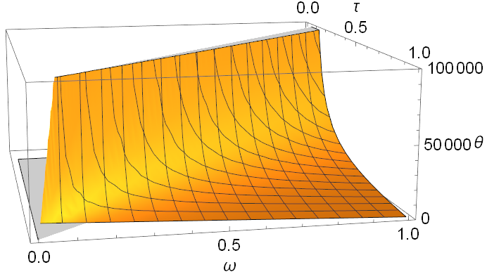
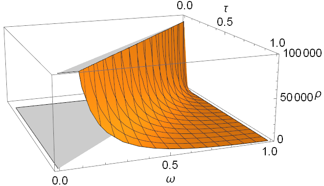
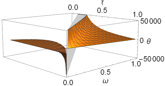
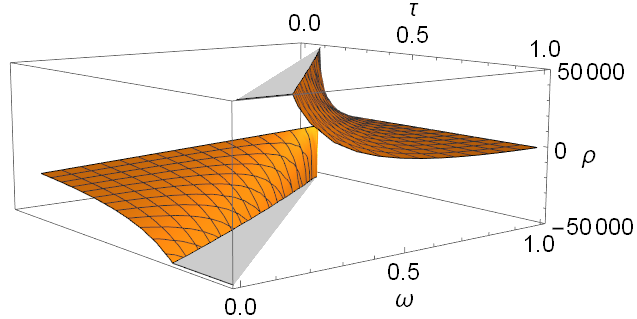
Figure 1: Solutions of Eq.(8) and Eq.(9) for $n=10000,\ \delta=.1,\ \omega\in(0,1)$.

Theorem 3.1

For any fair tax rule $\tau(\omega,\delta)\in(1-\omega+\delta\omega,1)$, as $n\to\infty$, $\tilde{p}_{n,\omega}$ converges in distribution to the degenerate probability distribution with mass at $\omega$.

4 AN ASYMPTOTIC RISK-FREE TAX RATE

In this section, we derive the limit fair tax rule $\tau(\omega,\delta)=1-\omega+\delta\omega$ from a few different angles. At a minimum, a good tax rule should not discourage employment incentives and productivity, such as detailed in Theorem 4.3 and 4.5. On the other end, we expect a good rule to be robust and optimal under multiple criteria. We study five criteria in Theorem 4.1, 4.2, 4.3, 4.4, and 4.6, any of which uniquely identifies the solution. They either minimize the employment market risk or maximize the employment expectation, under a given market capacity and a budget balance constraint.

First, we should heavily exploit the observed market behavior. While an efficient labor market stimulates productivity $v(\mathbf{S})$, a higher employment rate does not imply higher productivity and vice versa — the production function $v(\mathbf{S})$ does not necessarily increase with the employment size $|\mathbf{S}|$. Acemoglu and Shimer (2000) find that a moderate level of unemployment could boost productivity by improving the quality of jobs. Indeed, it fosters peer pressure in producing $v(\mathbf{S})$, allows workers to move on from declining firms, and enables rising companies and the economy as a whole to optimally respond to external shocks. Therefore, our tax rule would not merely target a higher expectation of employment rate, but grounds its assumption in the observed market behavior, and lets the market itself respond with a higher employment rate, to the maximum extent permitted by the budget rule and the market capacity.

Secondly, from a statistical viewpoint, our tax rule relies on a realization of $p$, not on the uncertainty of the realized value. A natural way to factor out this uncertainty is to study the posterior rate $\tilde{p}_{n,\omega}$, where both $s$ and $\omega$ are no longer random. As Theorem 3.1 indicates, $\omega$ is informative and indicative in revealing the central tendency of the posterior labor market, delineated by $\tilde{p}_{n,\omega}$. Asymptotic dispersion of $\tilde{p}_{n,\omega}$ and the market’s response to the tax rule $\tau(\omega,\delta)$ are among other essential ingredients in the complete profile of $\tilde{p}_{n,\omega}$. Thus, we set optimal criteria to minimize dispersion measures or maximize the expected market response.

4.1 Zero Asymptotic Posterior Variance

Tax rate stability creates the right environment for a balance of payments, reduces the uncertainty of the labor market, and creates confidence in technology and human capital investment. As a function of $\omega$, $\tau$ migrates the risk from the unemployment rate to the tax rate. With the absence of other exogenous shocks, indeed, stability in the tax rate is equivalent to that in the unemployment rate. The same argument is also valid when the exogenous shocks are orthogonal to that in $\omega$.

When we use the variance of $\tilde{p}_{n,\omega}$ to measure its instability, Theorem 4.1 states that the tax rule $\tau(\omega,\delta)=1-\omega+\delta\omega$ minimizes the asymptotic variance of $\tilde{p}_{n,\omega}$. Furthermore, it is also the limit of variance-minimizing tax rules for finite labor markets. We add the restriction “$\theta,\rho\geq\frac{1}{n}$” in the finite labor markets to ensure the positivity of the hyperparameters $(\theta,\rho)$.

Theorem 4.1

As $n\to\infty$, the tax rule $\tau(\omega,\delta)=1-\omega+\delta\omega$ minimizes the limit variance of $\sqrt{n}\tilde{p}_{n,\omega}$, i.e., $\mathop{\mathrm{argmin}}\limits_{\tau}\lim\limits_{n\to\infty}\mathrm{VAR}\left(\sqrt{n}\tilde{p}_{n,\omega}\right)=1-\omega+\delta\omega.$ Besides,
$\lim\limits_{n\to\infty}\mathop{\mathrm{argmin}}\limits_{\tau}\mathrm{VAR}\left(\sqrt{n}\tilde{p}_{n,\omega}\bigm{|}\theta,\rho\geq\frac{1}{n}\right)=1-\omega+\delta\omega.$ Furthermore, both the minimum limit variance and the limit minimum variance are zero.

We provide a few comments to help clarify any potential misunderstandings about the theorem. First, a stable $\sqrt{n}\tilde{p}_{n,\omega}$ is achieved at $n=\infty$ where the limit variance is zero. However, $\tilde{p}_{n,\omega}$ is still exposed to exogenous shocks, such as those studied in Pissarides (1992) and Blanchard (2000). Secondly, it is worth emphasizing that $1-\omega+\delta\omega$ is the limit tax rule as $n\to\infty$. For a large but finite $n$, a small positive number could be added to $1-\omega+\delta\omega$ to ensure the positivity of $\theta$ and $\rho$. That small positive number, however, is negligible; thus, we can practically use the rule $\tau(\omega,\delta)=1-\omega+\delta\omega$ without any addition. Moreover, a higher-order approximation $\tau=1-\omega+\delta\omega+\frac{\omega(1-\omega)(1-\delta)^{2}}{n}$ could be an excellent alternative to $\tau=1-\omega+\delta\omega$. Thirdly, with a zero or near zero variance in the unemployment rate, labor mobility means one layoff and one new hire should almost coincide to ensure the total employment size $|\mathbf{S}|$ remains nearly constant. It also means that the sizes of employment and labor market change proportionally so that their ratio remains unchanged. Lastly, though the posterior distribution is skewed, the tax rule minimizes both the overall risk and the one-sided risk of $\sqrt{n}\tilde{p}_{n,\omega}$, as stated in Theorem 4.2. In particular, a policymaker’s concern is on the downside risk only.

Theorem 4.2

As $n\to\infty$, the tax rule $\tau(\omega,\delta)=1-\omega+\delta\omega$ minimizes both the limit lower semivariance and the limit upper semivariance of $\sqrt{n}\tilde{p}_{n,\omega}$.

4.2 Consistency and Robustness

The above fair tax rule also captures several striking features of the labor market. In the first place, it is the policymaker’s best response to the market to stimulate employment within the framework of Eq.(8) and Eq.(9). In the second place, we can also derive it by minimizing statistical dispersion measures other than the posterior variance or semivariance. Meanwhile, it helps mitigate income inequality.

The rule $\tau(\omega,\delta)=1-\omega+\delta\omega$ is an effective taxation strategy to maximally boost the employment size without breaking the opportunity equality and the budget balance. For an economic policymaker, one primary concern is the forward-looking employment profile $\tilde{p}_{n,\omega}$. By Theorem 3.1, the mean of $\tilde{p}_{n,\omega}$ converges to $\omega$ as $n\to\infty$ for any fair rule $\tau(\omega,\delta)\in(1-\omega+\delta\omega,1)$. When $n$ is finitely large, they respond adversely to an increasing $\tau$ (cf Theorem 4.3). Consequently, to maximize the posterior mean, we should minimize the tax rate $\tau$ while still maintaining the conditions $\tau(\omega,\delta)\in(1-\omega+\delta\omega,1)$, $\theta>0$ and $\rho>0$. Thus, the limit of fair tax rates which maximize the mean of $\tilde{p}_{n,\omega}$ would be $1-\omega+\delta\omega$. As a remark, the condition $\omega>.5$ in Theorem 4.3 is satisfied in the general economy.

Theorem 4.3

For any $\omega\in(.5,1)$ and a finitely large $n$, the mean of $\tilde{p}_{n,\omega}$ reacts negatively to an increasing tax rate $\tau\in(1-\omega+\delta\omega,1)$. As a consequence,

$$\lim\limits_{n\to\infty}\mathop{\mathrm{argmax}}\limits_{\tau}\mathrm{MEAN}\left(\tilde{p}_{n,\omega}\bigm{|}\theta,\rho\geq\frac{1}{n}\right)=1-\omega+\delta\omega.$$

Furthermore, the tax rule also minimizes the mean absolute deviation (thereafter, MAD) from the mean as $n\to\infty$. For a Beta distribution, especially with large parameters, MAD is a more robust measure of statistical dispersion than the variance. The MAD around the mean for the posterior $\tilde{p}_{n,\omega}$ is (e.g., Gupta and Nadarajah 2004, page 37):

$$\mathbb{E}\left[\left|\tilde{p}_{n,\omega}-\mathbb{E}(\tilde{p}_{n,\omega})\right|\right]=\frac{2(\theta+s)^{\theta+s}(\rho+n-s)^{\rho+n-s}}{\beta(\theta+s,\rho+n-s)(\theta+\rho+n)^{\theta+\rho+n}}.$$ (10)

In the next theorem, we identify the same tax rule by minimizing the asymptotic MAD.

Theorem 4.4

As $n\to\infty$, the tax rule $\tau(\omega,\delta)=1-\omega+\delta\omega$ minimizes the MAD of $n\tilde{p}_{n,\omega}$ around the mean, i.e. $\lim\limits_{n\to\infty}\mathop{\mathrm{argmin}}\limits_{\tau}\mathbb{E}\left[n\left|\tilde{p}_{n,\omega}-\mathbb{E}(\tilde{p}_{n,\omega})\right|\biggm{|}\theta,\rho\geq\frac{1}{n}\right]=1-\omega+\delta\omega.$ Besides, $\mathop{\mathrm{argmin}}\limits_{\tau}\lim\limits_{n\to\infty}\mathbb{E}\left[n\left|\tilde{p}_{n,\omega}-\mathbb{E}(\tilde{p}_{n,\omega})\right|\biggm{|}\theta,\rho\geq\frac{1}{n}\right]=1-\omega+\delta\omega.$

4.3 Equality of Outcome with Symmetric Production

To see the relation between productivity and the tax rate, we introduce a partial ordering in the labor market. For any $i,j\in\mathbb{N}$ with $i\not=j$, we say $i$ uniformly outperforms $j$ in $v$ if

• $v(T\cup\overline{i})-v(T)\geq v(T\cup\overline{j})-v(T)$ for any $T\subseteq\mathbb{N}\setminus\overline{i}\setminus\overline{j}$; and

• $v(T)-v(T\setminus\overline{i})\geq v(T)-v(T\setminus\overline{j})$ for any $T\subseteq\mathbb{N}$ with $i,j\in T$.

With these two inequality conditions, $i$ has higher marginal productivity than $j$ in all comparable employment contingencies $-$ either both employed or both unemployed. As productivity is highly valued in Eq.(4) and Eq.(5), $j$ should receive fewer employment benefits and less unemployment welfare than $i$ does. This is formally claimed in Theorem 4.5. Besides, the theorem does not require the Beta-Binomial distribution, as long as $i$ and $j$ alone have the same chance of being employed; other players in the labor market may have unequal employment opportunities. The theorem is valid for all fair tax rules, including the special one $\tau(\omega,\delta)=1-\omega+\delta\omega$.

Theorem 4.5

If $i\in\mathbb{N}$ uniformly outperforms $j\in\mathbb{N}$ in $v$ and they have equal employment opportunity, then $\gamma_{i}[v]\geq\gamma_{j}[v]$ and $\lambda_{i}[v]\geq\lambda_{j}[v]$.

We say $i,j\in\mathbb{N}$ are symmetric in the production function $v$ if they uniformly outperform each other. By Theorem 4.5, $\lambda_{i}[v]=\lambda_{j}[v]$ and $\gamma_{i}[v]=\gamma_{j}[v]$ if $i$ and $j$ are symmetric and they have equal employment opportunity. In other words, they should receive the same amount of unemployment welfare if both are unemployed; they should also receive the same amount of employment benefits if both are employed.

Without any further analysis of or any prior knowledge about the production function, symmetry among the unemployed (or the employed) could be a reasonable a priori assumption to distribute the unemployment welfare (or employment benefits, respectively). For example, the Cobb-Douglas production function is symmetric among all employed persons in the labor market. Besides, if we assume symmetry among the employed labor and also assume symmetry among the unemployed labor, then the tax rule $\tau(\omega,\delta)=1-\omega+\delta\omega$ eliminates the income inequality, when the income is either employment benefits or unemployment welfare. Theorem 4.6 affirms this equality of outcome, but an employed individual and an unemployed one may not be symmetric in $v$. Furthermore, the theorem does not restrict the size of $n$ and the specific probability distribution for the equal employment opportunity. In the $k$-out-of-$n$ redundant system mentioned in Section 1, accordingly, the $n$ components (either working or standby) are equally important if they have equal quality. Section 6 offers a few alternative probability distributions for the equal employment opportunity.

Theorem 4.6

Assume equal employment opportunity in $\mathbb{N}$. If all employed individuals are symmetric in $v$ and all unemployed individuals are also symmetric in $v$, then $\tau(\omega,\delta)=1-\omega+\delta\omega$ if and only if an unemployed person’s unemployment welfare equals an employee’s employment benefits.

4.4 Labor Cost

We could use the symmetry to calibrate the labor cost, which is excluded from $v({\mathbf{S}})$. For example, let the labor cost for $i\in{\mathbf{S}}$ be the minimum wage requirement from all $j\in\mathbb{N}\setminus{\mathbf{S}}$, who either are symmetric with $i$ or uniformly outperforms $i$ in $v$. That is, some $j$ from $\mathbb{N}\setminus{\mathbf{S}}$ can do $i$’s work without compromising the production $v$. The minimum wage is called reservation wage, below which $j$ is unwilling to work. At this minimum market replacement cost, ${\mathbf{S}}$ can switch $i$ with someone else from $\mathbb{N}\setminus{\mathbf{S}}$ without sacrificing its net profit.

In fact, $j$ does not need to be symmetric with or outperform $i$ as long as the probability of $v({\mathbf{S}}\cup\overline{j}\setminus\overline{i})\geq v({\mathbf{S}}\cup\overline{i}\setminus\overline{j})$ is significantly large and the person has a willingness to accept (e.g., Horowitz and McConnell 2003). The probability of such $\mathbf{S}$ could be difficult for job interviewers to approximate and estimate.

At the other end, in order to avoid creating an undue disincentive to work, $j$’s unemployment welfare must be less than the reservation wage plus employment benefit. Moreover, to ensure every one of $\mathbb{N}$ is in the labor market, the welfare is necessary to bind to the incentive-compatibility constraint. This incentive requirement places a lower bound for the labor cost.

5 OTHER APPLICATIONS

In an abstract sense, the above account is a fair-division solution for the following game-theoretic setting: there are a large number of players; the players are randomly divided into two groups; the payoff comes from one group. A wide range of applications falls into this type of games. In this section, we analyze three applications other than labor markets to show how to use the formula derived in the last three sections.

5.1 Voting Power

In a voting game (e.g., Shapley 1962), $v:2^{\mathbb{N}}\to\{0,1\}$ is a monotonically increasing set function. Let $\mathbf{S}$ denote the random subset of voters who vote for the proposal. The proposal passes when $v(\mathbf{S})=1$; otherwise, it blocks when $v(\mathbf{S})=0$. However, $v$ should not mean “production” or alike.

No matter the outcome, Hu (2006) describes $\gamma_{i}[v]$ as $i$’s probability of turning a blocked result to a passed one, and $\lambda_{i}[v]$ the probability of turning a passed result to being blocked. Thus, the sum of $\lambda_{i}[v]$ and $\gamma_{i}[v]$ quantifies $i$’s power in the game.

The ratio $\delta$ plays a role in some circumstances. Let us consider, for example, $10\%$ of the voters approve just a proposal before a referendum voting on the proposal, and assume the number of other voters’ support ballots follows a Beta-Binomial distribution.

Many voting games are symmetric. In these cases, the equality of outcome becomes an egalitarian allocation of power.

5.2 Health Insurance

Health insurance has two types of policyholders: some are ill and use the insurance to cover their medical expenses; others are healthy and do not use the insurance. Let $\mathbf{S}$ denote the random set of ill policyholders, $v(\mathbf{S})$ be the total medical expenses with copays deducted, and $\tilde{\delta}v(\mathbf{S})$ be the surcharge paid to the insurance company. Let $\delta=-\tilde{\delta}$. Then the total expenses except for the copays, $(1-\delta)v(\mathbf{S})$, are billed to all insurance policyholders.

If $\tau=1-\omega+\delta\omega$ and $v$ is symmetric among the two types of policyholders, respectively, then by the equality of outcome, the cost to buy the insurance policy would be $\frac{(1-\delta)\mathbb{E}\left[v(\mathbf{S})\right]}{n}$ per policyholder. We take expectation on $\frac{(1-\delta)v(\mathbf{S})}{n}$ because the policyholders pay it upfront. On the contrary, the unemployment welfare and employment benefits payments come after the production.

In this example, patients pay the predetermined copays. In the labor market studied before, the labor costs are exempt from the distribution of the net production; they, however, have an indirect effect on $\tau$ through the corporate earning ratio and $\delta$. In the next example, we use the equality of outcome to derive the same type of payments as copays and labor cost.

5.3 Highway Toll

The I-66 highway inside the Capital Beltway of the Washington metropolitan area has enforced a dynamic toll rule during rush hours: a carpool driver pays no toll, but a solo driver pays a dynamic toll fee, say $\xi(n,\omega)$. Here $n$ is the number of cars in the segment of the highway, and $\omega$ is the percentage of solo drivers in the traffic.

Let $g(n)$ be the average carpool driver’s cost in the traffic when the traffic volume is $n$ cars. It is likely a nonlinear increasing function of $n$. An excellent choice of $g(n)$ is the expected driving time in hours multiplied by the average hourly pay rate, plus expenses on gas and vehicle depreciation. Also, let $\mathbf{S}$ denote the random set of solo drivers. Then, $v(\mathbf{S})=ng(n)-n(1-\omega)g\left(n(1-\omega)\right)-n\omega\xi(n,\omega)$ is the total cost of over-traffic generated by the solo drivers, with toll fees deducted.

The production function $v$ is symmetric among all solo drivers and also symmetric among all carpool drivers. By the equality of outcome, each driver shares the same cost $\frac{v(\mathbf{S})}{n}$. As a carpool driver pays no toll, his or her shared cost should exactly offset the extra cost caused by the solo drivers, which is $g(n)-g\left(n(1-\omega)\right)$. Finally, equation $\frac{v(\mathbf{S})}{n}=g(n)-g\left(n(1-\omega)\right)$ implies $\xi(n,\omega)=g\left(n(1-\omega)\right).$

In this example, an administration surcharge $\delta$ may apply; the carpooled passengers are free-riders, but their costs are exempt from $v(\mathbf{S})$.

6 CONCLUSIONS

In this paper, a fair-division solution is proposed to allocate the unemployment welfare in an economy, where the heterogeneous-agent production function is almost unknown. We interpret “fairness” as equal employment opportunity and model it by a Beta-Binomial probability distribution. Our “sustainability” is meant to be free of debt and free of surplus in the taxation budget. To justify the value of the unemployed labor, we capitalize on the D-value concept in Hu (2018). The D-value specifies how much of the net production to be retained with the employed labor, and what portion to be distributed to the unemployed. Finally, we postulate that the labor market is static and identify a sustainable tax policy by minimizing the asymptotic variance of the posterior employment rate. The policy can also be uniquely determined by minimizing the asymptotic posterior mean of the unemployment rate, or minimizing the downside risk of the posterior employment rate, or minimizing the posterior mean absolute deviation. Surprisingly, the tax rule is not only simple enough for practical use but also motivates the unemployed to seek employment and the employed to improve productivity.

One could extend this framework in several ways. One way is to re-specify the probability distribution of equal employment opportunity, for example, by any of the following re-specifications. First, we can replace the two-parameter Beta distribution with a four-parameter one or a Beta rectangular distribution. Secondly, we can let $\theta$ and $\rho$ be some functions of other unknown parameters. Thirdly, we could substitute the Beta-Binomial distribution with a Dirichlet-Multinomial distribution or a Beta-Geometric distribution. Fourthly, we could randomize $p$ without involving $(\theta,\rho)$, by generating two independent three-parameter Gamma random variables $X$ and $Y$. Then, the ratio $X/(X+Y)$ is a Beta random variable. In any of the four cases, however, we need additional identification restrictions to figure out a $\tau(\omega,\delta)$ precisely.

From other angles, we could apply other identification schemes or other objective functions to find a unique fair tax rule. From a statistical viewpoint, one could try the maximum likelihood estimation using the twelve months’ data prior to determining the policy tax rate, or minimize the ex-ante risk of $\omega$, or apply the statistical methods mentioned in Section 3.2. From an economic viewpoint, one could minimize the Gini coefficient of the Beta distribution of $\tilde{p}_{n,\omega}$. From a strategic game-theoretical viewpoint, one could seek a bargaining solution from the feasible solution set $\Omega_{n,\omega,\delta}$, which may be particularly useful when $n$ is small. Finally, a policymaker could treat the reserve ratio $\delta$ as endogenous, for example, letting it be an increasing function of $\omega$. He or she could also place a heavier weight on the marginal gain than on the marginal loss, in order to stimulate employment.

The simple static model, however, ignores several important aspects of a real labor market. First, it does not capture the dynamic features of the income inequality, nor its rational response to the tax rule. Secondly, while preventing the fungibility of borrowing funds from the future reduces the risk that a government administration piles up its national debt, it impairs that administration’s ability (especially, monetary policy) to intervene in the economy. The government, however, can still moderately stimulate the economy during a recession by adjusting the reserve ratio $\delta$. Thirdly, the postulation of labor market efficiency does neglect the recent development of the incomplete-market theory (e.g., Magill and Quinzii 1996). Fourthly, a multi-criteria objective function may be a viable alternative to the minimum-variance one, especially when there is a high unemployment rate $1-\omega$ or a large $\delta$. Lastly, a single tax rule $\tau(\omega,\delta)$ could have overly simplified the complexity of the taxation system, which is also affected by other determinants. These are just a few challenges our framework introduces, which require further development.

In summary, the fair and sustainable tax policy studied here has a solid theoretical underpinning, together with simplicity in practical use, consistency with productivity and employment incentives, and robustness to similar objectives. When applying this framework to a real fair-division problem, one should also consider the benefits of alternative probability distributions for equal opportunity, alternative objective functions, alternative restrictions, and dynamic thinking.

APPENDIX

Our focus in this paper is to study the relationship between the fair tax rate $\tau$ and the employment rate $\omega$ when the labor market size $n$ is large. To analyze the limit behavior of $\tau$ and $\omega$ for a large $n$, we only need the relevant asymptotic approximations. We say two functions $f(n)=O\left(g(n)\right)$ if $\limsup\limits_{n\to\infty}\left|\frac{f(n)}{g(n)}\right|<\infty$; and we say $f(n)\approx g(n)$ if $\lim\limits_{n\to\infty}\frac{f(n)}{g(n)}=1$. For simplicity, let us denote the following shorthands:

$$\begin{array}[]{lcl}\Delta&\equiv&\omega+\tau-\delta\omega-1,\\ \Delta_{1}&\equiv&\delta\omega-\omega-\tau+2\equiv 1-\Delta,\\ \Delta_{2}&\equiv&\delta\omega\tau-2\delta\omega-\omega\tau^{2}+2\omega\tau+\tau-1,\\ \Delta_{3}&\equiv&(1-\tau)(\delta-\tau)=\delta-\tau-\delta\tau+\tau^{2},\\ \Delta_{4}&\equiv&-\delta\omega\tau+\delta\omega+\delta\tau-2\delta+\omega\tau^{2}-2\omega\tau+\omega-\tau^{2}+3\tau-1,\\ \Delta_{5}&\equiv&-\delta\omega+\delta\tau-2\delta+\omega-\tau^{2}+4\tau-2\equiv\Delta_{2}+\Delta_{4},\\ \Delta_{6}&\equiv&-\omega\delta+\omega\tau+\tau-1\equiv\Delta_{2}+\omega\Delta_{3},\\ \Delta_{7}&\equiv&-\delta-\omega\tau+2\tau+\omega-1\equiv\Delta_{4}+(1-\omega)\Delta_{3},\\ \Delta_{8}&\equiv&-\delta\omega-\delta+\omega+3\tau-2\equiv\Delta_{3}+\Delta_{5},\\ \Delta_{9}&\equiv&-2\delta\omega-\delta+2\omega+4\tau-3\equiv\Delta+\Delta_{8}.\par\end{array}$$

The following lemma, to be used in other proofs, re-writes Eq.(8) and Eq.(9).

Lemma 1

In terms of $(n,\delta,\tau,\omega)$, we can solve $(\theta,\rho)$ from Eq.(8) and Eq.(9) as

$$\left\{\begin{array}[]{l}\theta=\frac{n^{2}\omega\Delta_{1}+n\Delta_{2}+\Delta_{3}}{n\Delta+\Delta_{3}},\\ \rho=\frac{n^{2}(1-\omega)\Delta_{1}+n\Delta_{4}+\Delta_{3}}{n\Delta+\Delta_{3}}.\end{array}\right.$$ (A.1)

A1. Proof of Theorem 2.1

In this proof, we use the following relation about Beta functions:

$$\left\{\begin{array}[]{lcll}\beta(x-1,y+1)&=&\frac{y}{x-1}\beta(x,y),&x>1,\ y>0;\\ \beta(x+1,y-1)&=&\frac{x}{y-1}\beta(x,y),&x>0,\ y>1.\\ \end{array}\right.$$

First, the expected aggregate marginal gain and loss are:

$$\begin{array}[]{rcl}\mathbb{E}\left[\sum\limits_{i\in\mathbf{S}}\left(v(\mathbf{S})-v(\mathbf{S}\setminus\overline{i})\right)\right]\par&=&\sum\limits_{T\subseteq\mathbb{N}}\mathbb{P}(\mathbf{S}=T)\sum\limits_{i\in T}\left[v(T)-v(T\setminus\overline{i})\right]\\ &=&\sum\limits_{i\in\mathbb{N}}\sum\limits_{T\subseteq\mathbb{N}:i\in T}\mathbb{P}(\mathbf{S}=T)\left[v(T)-v(T\setminus\overline{i})\right]\\ &=&\sum\limits_{i\in\mathbb{N}}\gamma_{i}[v],\\ \mathbb{E}\left[\sum\limits_{i\in\mathbb{N}\setminus\mathbf{S}}\left(v(\mathbf{S}\cup\overline{i})-v(\mathbf{S})\right)\right]\par&=&\sum\limits_{T\subseteq\mathbb{N}}\mathbb{P}(\mathbf{S}=T)\sum\limits_{i\in\mathbb{N}\setminus T}\left[v(T\cup\overline{i})-v(T)\right]\\ &=&\sum\limits_{i\in\mathbb{N}}\sum\limits_{T\subseteq\mathbb{N}:i\not\in T}\mathbb{P}(\mathbf{S}=T)\left[v(T\cup\overline{i})-v(T)\right]\\ &=&\sum\limits_{i\in\mathbb{N}}\lambda_{i}[v].\par\end{array}$$

Next, by Eq.(3)$-$(5), we re-write the expected marginal gain and loss as:

$$\begin{array}[]{rcl}\gamma_{i}[v]&=&\sum\limits_{T\subseteq\mathbb{N}:T\ni i}\frac{\beta(\theta+t,\rho+n-t)}{\beta(\theta,\rho)}[v(T)-v(T\setminus\overline{i})]\\ &\stackrel{{\scriptstyle Z=T\setminus\overline{i}}}{{=}}&\sum\limits_{T\subseteq\mathbb{N}:T\ni i}\frac{\beta(\theta+t,\rho+n-t)}{\beta(\theta,\rho)}v(T)-\sum\limits_{Z\subseteq\mathbb{N}\setminus\overline{i}}\frac{\beta(\theta+|Z|+1,\rho+n-|Z|-1)}{\beta(\theta,\rho)}v(Z),\\ \lambda_{i}[v]&=&\sum\limits_{Z\subseteq\mathbb{N}\setminus\overline{i}}\frac{\beta(\theta+|Z|,\rho+n-|Z|)}{\beta(\theta,\rho)}[v(Z\cup\overline{i})-v(Z)]\\ &\stackrel{{\scriptstyle T=Z\cup\overline{i}}}{{=}}&\sum\limits_{T\subseteq\mathbb{N}:T\ni i}\frac{\beta(\theta+t-1,\rho+n-t+1)}{\beta(\theta,\rho)}v(T)-\sum\limits_{Z\subseteq\mathbb{N}\setminus\overline{i}}\frac{\beta(\theta+|Z|,\rho+n-|Z|)}{\beta(\theta,\rho)}v(Z).\end{array}$$ (A.2)

By Eq.(A.2), the aggregate value of the employed labor $\sum\limits_{i\in\mathbb{N}}\gamma_{i}[v]$ is

$$\begin{array}[]{rcl}&&\sum\limits_{i\in\mathbb{N}}\sum\limits_{T\subseteq\mathbb{N}:T\ni i}\frac{\beta(\theta+t,\rho+n-t)}{\beta(\theta,\rho)}v(T)-\sum\limits_{i\in\mathbb{N}}\sum\limits_{Z\subseteq\mathbb{N}\setminus\overline{i}}\frac{\beta(\theta+|Z|+1,\rho+n-|Z|-1)}{\beta(\theta,\rho)}v(Z)\\ &\stackrel{{\scriptstyle T=Z}}{{=}}&\sum\limits_{T\subseteq\mathbb{N}:T\not=\emptyset}\sum\limits_{i\in T}\frac{\beta(\theta+t,\rho+n-t)}{\beta(\theta,\rho)}v(T)-\sum\limits_{T\subseteq\mathbb{N}:T\not=\mathbb{N}}\sum\limits_{i\in\mathbb{N}\setminus T}\frac{\beta(\theta+t+1,\rho+n-t-1)}{\beta(\theta,\rho)}v(T)\\ &=&\sum\limits_{T\subseteq\mathbb{N}:T\not=\emptyset}\frac{t\beta(\theta+t,\rho+n-t)}{\beta(\theta,\rho)}v(T)-\sum\limits_{T\subseteq\mathbb{N}:T\not=\mathbb{N}}\frac{(n-t)\beta(\theta+t+1,\rho+n-t-1)}{\beta(\theta,\rho)}v(T)\\ &=&\frac{n\beta(\theta+n,\rho)}{\beta(\theta,\rho)}v(\mathbb{N})-\frac{n\beta(\theta+1,\rho+n-1)}{\beta(\theta,\rho)}v(\emptyset)\\ &&+\sum\limits_{T\subseteq\mathbb{N}:T\not=\emptyset,T\not=\mathbb{N}}\frac{t\beta(\theta+t,\rho+n-t)-(n-t)\beta(\theta+t+1,\rho+n-t-1)}{\beta(\theta,\rho)}v(T)\\ &=&\frac{n\beta(\theta+n,\rho)}{\beta(\theta,\rho)}v(\mathbb{N})-\frac{n\theta}{\rho+n-1}\frac{\beta(\theta,\rho+n)}{\beta(\theta,\rho)}v(\emptyset)\\ &&+\sum\limits_{T\subseteq\mathbb{N}:T\not=\mathbb{N},T\not=\emptyset}\left[t-\frac{(n-t)(\theta+t)}{\rho+n-t-1}\right]\frac{\beta(\theta+t,\rho+n-t)}{\beta(\theta,\rho)}v(T)\\ &=&\frac{n\beta(\theta+n,\rho)}{\beta(\theta,\rho)}v(\mathbb{N})+\sum\limits_{T\subseteq\mathbb{N}:T\not=\mathbb{N}}\frac{t(\theta+\rho-1)-n\theta}{\rho+n-t-1}\frac{\beta(\theta+t,\rho+n-t)}{\beta(\theta,\rho)}v(T).\par\end{array}$$

Also by Eq.(A.2), the aggregate value of the unemployed labor $\sum\limits_{i\in\mathbb{N}}\lambda_{i}[v]$ is

$$\begin{array}[]{rcl}&&\sum\limits_{i\in\mathbb{N}}\sum\limits_{T\subseteq\mathbb{N}:T\ni i}\frac{\beta(\theta+t-1,\rho+n-t+1)}{\beta(\theta,\rho)}v(T)-\sum\limits_{i\in\mathbb{N}}\sum\limits_{Z\subseteq\mathbb{N}\setminus\overline{i}}\frac{\beta(\theta+|Z|,\rho+n-|Z|)}{\beta(\theta,\rho)}v(Z)\\ &\stackrel{{\scriptstyle T=Z}}{{=}}&\sum\limits_{T\subseteq\mathbb{N}:T\not=\emptyset}\sum\limits_{i\in T}\frac{\beta(\theta+t-1,\rho+n-t+1)}{\beta(\theta,\rho)}v(T)-\sum\limits_{T\subseteq\mathbb{N}:T\not=\mathbb{N}}\sum\limits_{i\in\mathbb{N}\setminus T}\frac{\beta(\theta+t,\rho+n-t)}{\beta(\theta,\rho)}v(T)\\ &=&\sum\limits_{T\subseteq\mathbb{N}:T\not=\emptyset}\frac{t\beta(\theta+t-1,\rho+n-t+1)}{\beta(\theta,\rho)}v(T)-\sum\limits_{T\subseteq\mathbb{N}:T\not=\mathbb{N}}\frac{(n-t)\beta(\theta+t,\rho+n-t)}{\beta(\theta,\rho)}v(T)\\ &=&\frac{n\beta(\theta+n-1,\rho+1)}{\beta(\theta,\rho)}v(\mathbb{N})-\frac{n\beta(\theta,\rho+n)}{\beta(\theta,\rho)}v(\emptyset)\\ &&+\sum\limits_{T\subseteq\mathbb{N}:T\not=\emptyset,T\not=\mathbb{N}}\frac{t\beta(\theta+t-1,\rho+n-t+1)-(n-t)\beta(\theta+t,\rho+n-t)}{\beta(\theta,\rho)}v(T)\\ &=&\frac{n\rho}{\theta+n-1}\frac{\beta(\theta+n,\rho)}{\beta(\theta,\rho)}v(\mathbb{N})-\frac{n\beta(\theta,\rho+n)}{\beta(\theta,\rho)}v(\emptyset)\\ &&+\sum\limits_{T\subseteq\mathbb{N}:T\not=\emptyset,T\not=\mathbb{N}}\left[\frac{t(\rho+n-t)}{\theta+t-1}-(n-t)\right]\frac{\beta(\theta+t,\rho+n-t)}{\beta(\theta,\rho)}v(T)\\ &=&\sum\limits_{T\subseteq\mathbb{N}:T\not=\emptyset}\frac{t(\theta+\rho-1)-n(\theta-1)}{\theta+t-1}\frac{\beta(\theta+t,\rho+n-t)}{\beta(\theta,\rho)}v(T)-\frac{n\beta(\theta,\rho+n)}{\beta(\theta,\rho)}v(\emptyset).\end{array}$$

∎

A2. Proof of Lemma 1

We can re-write Eq.(8) and Eq.(9) as a linear system of unknowns $(\theta,\rho)$:

$$\left\{\begin{array}[]{rcl}(1-\tau)(\rho+n-s-1)&=&s(\theta+\rho-1)-n\theta,\\ (\tau-\delta)(\theta+s-1)&=&s(\theta+\rho-1)-n(\theta-1).\end{array}\right.$$

As a consequence, the symbolic solution of $(\theta,\rho)$ is unique.

Let us assume Eq.(A.1) and verify that it satisfies both Eq.(8) and Eq.(9) by the following identities, some of which are used in other proofs:

$$\begin{array}[]{rcl}\theta+s&=&\frac{n^{2}\omega\Delta_{1}+n\Delta_{2}+\Delta_{3}}{n\Delta+\Delta_{3}}+\frac{n\omega(n\Delta+\Delta_{3})}{n\Delta+\Delta_{3}}=\frac{n^{2}\omega+n\Delta_{6}+\Delta_{3}}{n\Delta+\Delta_{3}},\\ \theta+s-1&=&\frac{n^{2}\omega+n\Delta_{6}+\Delta_{3}}{n\Delta+\Delta_{3}}-\frac{n\Delta+\Delta_{3}}{n\Delta+\Delta_{3}}=\frac{n^{2}\omega+n(\Delta_{6}-\Delta)}{n\Delta+\Delta_{3}}=\frac{n^{2}\omega+n\omega(\tau-1)}{n\Delta+\Delta_{3}},\\ \theta+\rho&=&\frac{n^{2}\omega\Delta_{1}+n\Delta_{2}+\Delta_{3}}{n\Delta+\Delta_{3}}+\frac{n^{2}(1-\omega)\Delta_{1}+n\Delta_{4}+\Delta_{3}}{n\Delta+\Delta_{3}}=\frac{n^{2}\Delta_{1}+n\Delta_{5}+2\Delta_{3}}{n\Delta+\Delta_{3}},\\ \theta+\rho-1&=&\frac{n^{2}\Delta_{1}+n\Delta_{5}+2\Delta_{3}}{n\Delta+\Delta_{3}}-\frac{n\Delta+\Delta_{3}}{n\Delta+\Delta_{3}}=\frac{n^{2}\Delta_{1}+n(\delta\tau-2\delta-\tau^{2}+3\tau-1)+\Delta_{3}}{n\Delta+\Delta_{3}},\\ \theta+\rho+n&=&\frac{n^{2}\Delta_{1}+n\Delta_{5}+2\Delta_{3}}{n\Delta+\Delta_{3}}+\frac{n(n\Delta+\Delta_{3})}{n\Delta+\Delta_{3}}=\frac{n^{2}+n\Delta_{8}+2\Delta_{3}}{n\Delta+\Delta_{3}},\\ \theta+\rho+n+1&=&\frac{n^{2}+n\Delta_{8}+2\Delta_{3}}{n\Delta+\Delta_{3}}+\frac{n\Delta+\Delta_{3}}{n\Delta+\Delta_{3}}=\frac{n^{2}+n\Delta_{9}+3\Delta_{3}}{n\Delta+\Delta_{3}},\\ \theta+\rho+n-1&=&\frac{n^{2}+n\Delta_{8}+2\Delta_{3}}{n\Delta+\Delta_{3}}-\frac{n\Delta+\Delta_{3}}{n\Delta+\Delta_{3}}=\frac{n^{2}+n(\Delta_{8}-\Delta)+\Delta_{3}}{n\Delta+\Delta_{3}},\\ \theta+\rho+n-2&=&\frac{n^{2}+n\Delta_{8}+2\Delta_{3}}{n\Delta+\Delta_{3}}-\frac{2(n\Delta+\Delta_{3})}{n\Delta+\Delta_{3}}=\frac{n^{2}+n(\Delta_{8}-2\Delta)}{n\Delta+\Delta_{3}},\\ \rho+n-s&=&\frac{n^{2}(1-\omega)\Delta_{1}+n\Delta_{4}+\Delta_{3}}{n\Delta+\Delta_{3}}+\frac{n(1-\omega)(n\Delta+\Delta_{3})}{n\Delta+\Delta_{3}}=\frac{n^{2}(1-\omega)+n\Delta_{7}+\Delta_{3}}{n\Delta+\Delta_{3}},\\ \rho+n-s-1&=&\frac{n^{2}(1-\omega)+n\Delta_{7}+\Delta_{3}}{n\Delta+\Delta_{3}}-\frac{n\Delta+\Delta_{3}}{n\Delta+\Delta_{3}}=\frac{n^{2}(1-\omega)+n(1-\omega)(\tau-\delta)}{n\Delta+\Delta_{3}}.\par\end{array}$$

Thus,

$$\begin{array}[]{rcl}s(\theta+\rho-1)-n\theta&=&\frac{n\omega[n^{2}\Delta_{1}+n(\delta\tau-2\delta-\tau^{2}+3\tau-1)+\Delta_{3}]}{n\Delta+\Delta_{3}}\\ &&-\frac{n(n^{2}\omega\Delta_{1}+n\Delta_{2}+\Delta_{3})}{n\Delta+\Delta_{3}}\\ &=&\frac{n^{2}[\omega(\delta\tau-2\delta-\tau^{2}+3\tau-1)-\Delta_{2}]+n(\omega-1)\Delta_{3}}{n\Delta+\Delta_{3}}\\ &=&\frac{n^{2}(1-\omega)(1-\tau)+n(\omega-1)\Delta_{3}}{n\Delta+\Delta_{3}},\\ s(\theta+\rho-1)-n(\theta-1)&=&\left[s(\theta+\rho-1)-n\theta\right]+n\\ &=&\frac{n^{2}(1-\omega)(1-\tau)+n(\omega-1)\Delta_{3}}{n\Delta+\Delta_{3}}+\frac{n(n\Delta+\Delta_{3})}{n\Delta+\Delta_{3}}\\ &=&\frac{n^{2}\omega(\tau-\delta)+n\omega\Delta_{3}}{n\Delta+\Delta_{3}}.\\ \end{array}$$

Therefore,

$$\begin{array}[]{rclcl}\frac{s(\theta+\rho-1)-n\theta}{\rho+n-s-1}&=&\frac{n^{2}(1-\omega)(1-\tau)+n(\omega-1)\Delta_{3}}{n^{2}(1-\omega)+n(1-\omega)(\tau-\delta)}&=&1-\tau,\\ \frac{s(\theta+\rho-1)-n(\theta-1)}{\theta+s-1}&=&\frac{n^{2}\omega(\tau-\delta)+n\omega\Delta_{3}}{n^{2}\omega+n\omega(\tau-1)}&=&\tau-\delta,\end{array}$$

which are equivalent to Eq.(8) and Eq.(9), respectively. ∎

A3. Proof of Theorem 3.1

For any integer $z\geq 0$, by the proof of Lemma 1,

$$\begin{array}[]{rcl}\frac{\theta+s+z}{\theta+\rho+n+z}\par&=&\frac{\frac{n^{2}\omega+n\Delta_{6}+\Delta_{3}}{n\Delta+\Delta_{3}}+\frac{z(n\Delta+\Delta_{3})}{n\Delta+\Delta_{3}}}{\frac{n^{2}+n\Delta_{8}+2\Delta_{3}}{n\Delta+\Delta_{3}}+\frac{z(n\Delta+\Delta_{3})}{n\Delta+\Delta_{3}}}\\ &=&\frac{n^{2}\omega+n(\Delta_{6}+z\Delta)+(1+z)\Delta_{3}}{n^{2}+n(\Delta_{8}+z\Delta)+(2+z)\Delta_{3}}\\ &\to&\omega,\quad\mathrm{as}\ \ n\to\infty.\end{array}$$

As a function of $\eta$, the characteristic function of $\tilde{p}_{n,\omega}$ (e.g., Johnson et al. 1995, Chapter 21) is

$$\mathbb{E}\left[e^{i\eta\tilde{p}_{n,\omega}}\right]=1+\sum\limits_{k=1}^{\infty}\frac{(i\eta)^{k}}{k!}\prod\limits_{z=0}^{k-1}\frac{\theta+s+z}{\theta+\rho+n+z}$$

where $i$ is the unit imaginary number, i.e., $i^{2}=-1$. We let $n\to\infty$,

$$\begin{array}[]{rcl}\lim\limits_{n\to\infty}\mathbb{E}[e^{i\eta\tilde{p}_{n,\omega}}]&=&1+\sum\limits_{k=1}^{\infty}\frac{(i\eta)^{k}}{k!}\lim\limits_{n\to\infty}\prod\limits_{z=0}^{k-1}\frac{\theta+s+z}{\theta+\rho+n+z}\\ &=&1+\sum\limits_{k=1}^{\infty}\frac{(i\eta\omega)^{k}}{k!}\\ &=&\exp(i\eta\omega).\end{array}$$

Therefore, as $n\to\infty$, $\tilde{p}_{n,\omega}$ converges in distribution to the degenerate distribution with mass at $\omega$, which has the characteristic function $\exp(i\eta\omega)$. ∎

A4. Proof of Theorem 4.1

As $\tilde{p}_{n,\omega}$ has a Beta distribution with parameters $(\theta+s,\rho+n-s)$ (see Section 2.1), its variance is $\frac{(\theta+s)(\rho+n-s)}{(\theta+\rho+n)^{2}(\theta+\rho+n+1)}$ (e.g., Gupta and Nadarajah 2004, page 35). By the proof of Lemma 1, the variance of $\sqrt{n}\tilde{p}_{n,\omega}$ is

$$\begin{array}[]{rcl}&&\frac{n\frac{n^{2}\omega+n\Delta_{6}+\Delta_{3}}{n\Delta+\Delta_{3}}\frac{n^{2}(1-\omega)+n\Delta_{7}+\Delta_{3}}{n\Delta+\Delta_{3}}}{\left(\frac{n^{2}+n\Delta_{8}+2\Delta_{3}}{n\Delta+\Delta_{3}}\right)^{2}\frac{n^{2}+n\Delta_{9}+3\Delta_{3}}{n\Delta+\Delta_{3}}}\\ &=&\frac{n(n\Delta+\Delta_{3})(n^{2}\omega+n\Delta_{6}+\Delta_{3})\left[n^{2}(1-\omega)+n\Delta_{7}+\Delta_{3}\right]}{\left(n^{2}+n\Delta_{8}+2\Delta_{3}\right)^{2}\left(n^{2}+n\Delta_{9}+3\Delta_{3}\right)}\\ &=&\frac{\left(\Delta+\frac{\Delta_{3}}{n}\right)\left[\omega\left(1+\frac{\Delta_{6}}{n\omega}+\frac{\Delta_{3}}{n^{2}\omega}\right)\right]\left[(1-\omega)\left(1+\frac{\Delta_{7}}{n(1-\omega)}+\frac{\Delta_{3}}{n^{2}(1-\omega)}\right)\right]}{\left(1+\frac{\Delta_{8}}{n}+\frac{2\Delta_{3}}{n^{2}}\right)^{2}\left(1+\frac{\Delta_{9}}{n}+\frac{3\Delta_{3}}{n^{2}}\right)}\\ &=&\omega(1-\omega)\left(\Delta+\frac{\Delta_{3}}{n}\right)\left[1+\frac{\Delta_{6}}{n\omega}+\frac{\Delta_{7}}{n(1-\omega)}-\frac{2\Delta_{8}}{n}-\frac{\Delta_{9}}{n}+O\left(\frac{1}{n^{2}}\right)\right]\\ &=&\omega(1-\omega)\Delta+\frac{\omega(1-\omega)}{n}\left[\Delta_{3}+\Delta(\frac{\Delta_{6}}{\omega}+\frac{\Delta_{7}}{1-\omega}-2\Delta_{8}-\Delta_{9})\right]+O\left(\frac{1}{n^{2}}\right)\\ &\to&\omega(1-\omega)(\omega+\tau-\delta\omega-1),\qquad\mathrm{as}\ \ n\to\infty.\end{array}$$ (A.3)

To minimize $\lim\limits_{n\to\infty}\mathrm{VAR}(\sqrt{n}\tilde{p}_{n,\omega})=\omega(1-\omega)\Delta$ while $\lim\limits_{n\to\infty}\mathrm{VAR}(\sqrt{n}\tilde{p}_{n,\omega})\geq 0$, we have to set $\Delta=0$. Thus, $\mathop{\mathrm{argmin}}\limits_{\tau}\lim\limits_{n\to\infty}\mathrm{VAR}\left(\sqrt{n}\tilde{p}_{n,\omega}\right)=1-\omega+\delta\omega.$

However, when applying $\tau=1-\omega+\delta\omega$ to a labor market with finite $n$, we have $\Delta=0$, $\Delta_{1}=1$ and $\Delta_{3}=-\omega(1-\omega)(1-\delta)^{2}$. And Lemma 1 reduces to

$$\left\{\begin{array}[]{rcl}\theta&=&\frac{n^{2}\omega+n\Delta_{2}-\omega(1-\omega)(1-\delta)^{2}}{-\omega(1-\omega)(1-\delta)^{2}},\\ \rho&=&\frac{n^{2}(1-\omega)+n\Delta_{4}-\omega(1-\omega)(1-\delta)^{2}}{-\omega(1-\omega)(1-\delta)^{2}},\end{array}\right.$$

which converge to $-\infty$ as $n\to\infty$. In theory, therefore, for a large but finite $n$, we need to choose $\tau$ to be $1-\omega+\delta\omega$ plus a small positive number to ensure that $\theta>0$ and $\rho>0$. To estimate the small positive number, let us first try the higher-order approximation of

$$\tau=1-\omega+\delta\omega+\frac{c}{n},$$

for some constant $c>0$. Then

$$\begin{array}[]{lcl}\Delta&=&\frac{c}{n},\\ \Delta_{3}&=&\left[\omega(1-\delta)-\frac{c}{n}\right]\left[-(1-\omega)(1-\delta)-\frac{c}{n}\right]\\ &=&-\omega(1-\omega)(1-\delta)^{2}+O\left(\frac{1}{n}\right).\par\end{array}$$ (A.4)

By the next to the last step in (A.3),

$$\mathrm{VAR}\left(\sqrt{n}\tilde{p}_{n,\omega}\Bigm{|}\tau=1-\omega+\delta\omega+\frac{c}{n}\right)=\frac{\omega(1-\omega)c-\omega^{2}(1-\omega)^{2}(1-\delta)^{2}}{n}+O\left(\frac{1}{n^{2}}\right).$$

To minimize the above variance, we let $c=\omega(1-\omega)(1-\delta)^{2}$. Thus, $\tau=1-\omega+\delta\omega+\frac{\omega(1-\omega)(1-\delta)^{2}}{n}$ is a higher-order approximation for $1-\omega+\delta\omega$. Further high-order approximations, if necessary, could be found similarly.

When $\tau=1-\omega+\delta\omega+\frac{c}{n}$, let us use Eq.(A.4) to calculate

$$\begin{array}[]{rcl}n\Delta+\Delta_{3}&=&c+\left[\omega(1-\delta)-\frac{c}{n}\right]\left[-(1-\omega)(1-\delta)-\frac{c}{n}\right]\\ &=&\frac{(1-2\omega)(1-\delta)c}{n}+\frac{c^{2}}{n^{2}}\end{array}$$ (A.5)

which is negative when $\omega>.5$ and $n\geq\left|\frac{\omega(1-\omega)(1-\delta)}{1-2\omega}\right|$. As the numerators of $\theta$ and $\rho$ in Lemma 1 are both positive for a large $n$, $\theta$ and $\rho$ are negative when $n$ is large and $\omega>.5$.

Let us make another try at $\tau=1-\omega+\delta\omega+\frac{2c}{n}$. Similar to Eq.(A.5),

$$\begin{array}[]{rcl}n\Delta+\Delta_{3}&=&2c+\left[\omega(1-\delta)-\frac{2c}{n}\right]\left[-(1-\omega)(1-\delta)-\frac{2c}{n}\right]\\ &=&c+\frac{2(1-2\omega)(1-\delta)c}{n}+\frac{4c^{2}}{n^{2}}.\end{array}$$

In this case, both $\theta$ and $\rho$ are larger than $\frac{1}{n}$ when $n$ is large. Note from the last step of Eq.(A.3) that $\mathrm{VAR}\left(\sqrt{n}\tilde{p}_{n,\omega}\right)$ is an increasing function of $\tau$ when $n$ is large; thus, the small positive number to be added to $1-\omega+\delta\omega$ is between $\frac{c}{n}$ and $\frac{2c}{n}$. In practice, however, as the number is too small for a large $n$, there is no necessity to exactly calculate it and add it to $1-\omega+\delta\omega$.

Let $\tilde{\tau}_{n}=\mathop{\mathrm{argmin}}\limits_{\tau}\mathrm{VAR}\left(\sqrt{n}\tilde{p}_{n,\omega}\bigm{|}\theta,\rho\geq\frac{1}{n}\right)$. We add the restriction $\theta,\rho\geq\frac{1}{n}$ to ensure the existence of $\tilde{\tau}_{n}$. As $\mathrm{VAR}\left(\sqrt{n}\tilde{p}_{n,\omega}\right)$ is an increasing function of $\tau$ when $n$ is large, $\tilde{\tau}_{n}$ is unique and less than $1-\omega+\delta\omega+\frac{2c}{n}$ when $n$ is large. By Eq.(A.3),

$$\mathrm{VAR}(\sqrt{n}\tilde{p}_{n,\omega}\Bigm{|}\tau=\tilde{\tau}_{n})=\omega(1-\omega)(\omega+\tilde{\tau}_{n}-\delta\omega-1)+O\left(\frac{1}{n}\right).$$

Finally, we use the relation

$$0\leq\mathrm{VAR}\left(\sqrt{n}\tilde{p}_{n,\omega}\Bigm{|}\tau=\tilde{\tau}_{n}\right)\leq\mathrm{VAR}\left(\sqrt{n}\tilde{p}_{n,\omega}\Bigm{|}\tau=1-\omega+\delta\omega+\frac{2c}{n}\right)$$

to get

$$0\leq\omega(1-\omega)(\omega+\tilde{\tau}_{n}-\delta\omega-1)+O\left(\frac{1}{n}\right)\leq O\left(\frac{1}{n}\right).$$

Letting $n\to\infty$ in the above inequality, we get $\omega(1-\omega)(\omega+\tilde{\tau}_{n}-\delta\omega-1)=O(\frac{1}{n})$, i.e., $\lim\limits_{n\to\infty}\mathop{\mathrm{argmin}}\limits_{\tau}\mathrm{VAR}\left(\sqrt{n}\tilde{p}_{n,\omega}\bigm{|}\theta,\rho\geq\frac{1}{n}\right)=1-\omega+\delta\omega$. ∎

A5. Proof of Theorem 4.2

In this proof, we constantly apply the identities in the proof of Lemma 1. Let $\mu_{n}=\frac{\theta+s}{\theta+\rho+n}$ be the mean of $\tilde{p}_{n,\omega}$, and let $\sigma_{n}^{2}$ be the variance of $\tilde{p}_{n,\omega}$. The lower semivariance of $\tilde{p}_{n,\omega}$ is calculated as

$$\sigma^{2}_{n-}=\int_{0}^{\mu_{n}}(x-\mu_{n})^{2}\frac{x^{\theta+s-1}(1-x)^{\rho+n-s-1}}{\beta(\theta+s,\rho+n-s)}\mathrm{d}x.$$

We apply Chebychev’s inequality in terms of the lower semivariance (e.g., Berck and Hihn 1982) to get

$$\mathbb{P}\left(\tilde{p}_{n,\omega}\leq\mu_{n}-a_{n}\sigma_{n-}\right)\leq\frac{1}{a_{n}^{2}},\quad\forall\ a_{n}>0.$$

By the proof of Theorem 4.1, $\tilde{p}_{n,\omega}$ has the variance $\sigma_{n}^{2}=\frac{\omega(1-\omega)\Delta}{n}+O(\frac{1}{n^{2}})$. We let $a_{n}=\frac{\sqrt{\frac{\omega(1-\omega)\Delta}{n}}}{\sigma_{n-}}$, then

$$\mathbb{P}\left(\tilde{p}_{n,\omega}\leq\mu_{n}-\sqrt{\frac{\omega(1-\omega)\Delta}{n}}\right)\leq\frac{n\sigma^{2}_{n-}}{\omega(1-\omega)\Delta}.$$ (A.6)

Let $\kappa_{n}=\frac{\theta+s-1}{\theta+\rho+n-2}$ and $\varepsilon_{n}$ be the mode and median of $\tilde{p}_{n,\omega}$, respectively. The mode $\kappa_{n}$ maximizes the density function $\frac{x^{\theta+s-1}(1-x)^{\rho+n-s-1}}{\beta(\theta+s,\rho+n-s)},0<x<1$. As the median lies between the mean and mode, we have

$$\begin{array}[]{rcl}|\mu_{n}-\varepsilon_{n}|&\leq&|\mu_{n}-\kappa_{n}|=\left|\frac{\theta+s}{\theta+\rho+n}-\frac{\theta+s-1}{\theta+\rho+n-2}\right|\\ &=&\left|\frac{n+\rho-\theta-2s}{(\theta+\rho+n)(\theta+\rho+n-2)}\right|\\ &\leq&\left|\frac{\theta+s}{(\theta+\rho+n)(\theta+\rho+n-2)}\right|+\left|\frac{n+\rho-s}{(\theta+\rho+n)(\theta+\rho+n-2)}\right|\\ &=&O(\frac{1}{n}).\\ \end{array}$$

In the following lower-bound estimation of Eq.(A.6), we use Gamma function, denoted by $\Gamma(\cdot)$, and its Stirling’s approximation $\Gamma(z+1)\approx\sqrt{2\pi z}\left(\frac{z}{\exp(1)}\right)^{z}$.

$$\begin{array}[]{rcl}&&\mathbb{P}\left(\tilde{p}_{n,\omega}\leq\mu_{n}-\sqrt{\frac{\omega(1-\omega)\Delta}{n}}\right)\\ &=&\mathbb{P}\left(\tilde{p}_{n,\omega}\leq\varepsilon_{n}\right)-\int\limits_{\mu_{n}-\sqrt{\frac{\omega(1-\omega)\Delta}{n}}}^{\varepsilon_{n}}\frac{x^{\theta+s-1}(1-x)^{\rho+n-s-1}}{\beta(\theta+s,\rho+n-s)}\mathrm{d}x\\ &\geq&\frac{1}{2}-\left|\varepsilon_{n}-\left(\mu_{n}-\sqrt{\frac{\omega(1-\omega)\Delta}{n}}\right)\right|\frac{{\kappa_{n}}^{\theta+s-1}(1-\kappa_{n})^{\rho+n-s-1}}{\beta(\theta+s,\rho+n-s)}\\ &=&\frac{1}{2}-\left|\sqrt{\frac{\omega(1-\omega)\Delta}{n}}+O(\frac{1}{n})\right|\frac{\left(\frac{\theta+s-1}{\theta+\rho+n-2}\right)^{\theta+s-1}\left(1-\frac{\theta+s-1}{\theta+\rho+n-2}\right)^{\rho+n-s-1}}{\frac{\Gamma(\theta+s)\Gamma(\rho+n-s)}{\Gamma(\theta+\rho+n)}}\\ &=&\frac{1}{2}-\left|\sqrt{\frac{\omega(1-\omega)\Delta}{n}}+O(\frac{1}{n})\right|\frac{\frac{(\theta+s-1)^{\theta+s-1}}{\Gamma(\theta+s)}\frac{(\rho+n-s-1)^{\rho+n-s-1}}{\Gamma(\rho+n-s)}}{\frac{(\theta+\rho+n-2)^{\theta+\rho+n-2}}{(\theta+\rho+n-1)\Gamma(\theta+\rho+n-1)}}\\ &\approx&\frac{1}{2}-\sqrt{\frac{\omega(1-\omega)\Delta}{n}}\frac{\frac{\exp(\theta+s-1)}{\sqrt{2\pi(\theta+s-1)}}\frac{\exp(\rho+n-s-1)}{\sqrt{2\pi(\rho+n-s-1)}}}{\frac{\exp(\theta+\rho+n-2)}{(\theta+\rho+n-1)\sqrt{2\pi(\theta+\rho+n-2)}}}\\ &=&\frac{1}{2}-\sqrt{\frac{\omega(1-\omega)\Delta}{n}}\frac{(\theta+\rho+n-1)\sqrt{\theta+\rho+n-2}}{\sqrt{2\pi(\theta+s-1)(\rho+n-s-1)}}\\ &\approx&\frac{1}{2}-\sqrt{\frac{\omega(1-\omega)\Delta}{n}}\frac{\frac{n}{\Delta}\sqrt{\frac{n}{\Delta}}}{\sqrt{2\pi\frac{n\omega}{\Delta}\frac{n(1-\omega)}{\Delta}}}\\ &=&\frac{1}{2}-\frac{1}{\sqrt{2\pi}}.\end{array}$$

Finally, we re-write Eq.(A.6) as

$$\left(\frac{1}{2}-\frac{1}{\sqrt{2\pi}}\right)\omega(1-\omega)\Delta+O\left(\frac{1}{\sqrt{n}}\right)\leq n\sigma^{2}_{n-}\leq n\sigma_{n}^{2}=\omega(1-\omega)\Delta+O\left(\frac{1}{n}\right).$$

Letting $n\to\infty$, we get

$$\left(\frac{1}{2}-\frac{1}{\sqrt{2\pi}}\right)\omega(1-\omega)\Delta\leq\liminf\limits_{n\to\infty}n\sigma_{n-}^{2}\leq\limsup\limits_{n\to\infty}n\sigma_{n-}^{2}\leq\omega(1-\omega)\Delta.$$

Therefore, $\Delta=0$ minimizes the limit of lower semivariance of $\sqrt{n}\tilde{p}_{n,\omega}$.

We can apply similar arguments to the upper semivariance of $\sqrt{n}\tilde{p}_{n,\omega}$. ∎

A6. Proof of Theorem 4.3

Note that $\Delta_{6}-\omega\Delta_{8}=(1-\tau)(2\omega-1)+\omega^{2}(\delta-1).$ By the proof of Lemma 1,

$$\begin{array}[]{rcl}\mathbb{E}[\tilde{p}_{n,\omega}]&=&\frac{\theta+s}{\theta+\rho+n}=\frac{n^{2}\omega+n\Delta_{6}+\Delta_{3}}{n^{2}+n\Delta_{8}+2\Delta_{3}}\\ &=&\omega+\frac{n(\Delta_{6}-\omega\Delta_{8})+(1-2\omega)\Delta_{3}}{n^{2}+n\Delta_{8}+2\Delta_{3}}\\ &=&\omega+\frac{(1-\tau)(2\omega-1)+\omega^{2}(\delta-1)}{n}+O(\frac{1}{n^{2}}).\par\end{array}$$

In the above approximation, the mean reacts negatively with an increasing $\tau$, when $n$ is finitely large and $\omega>.5$. To maximize the mean, we thus minimize $\tau\in(1-\omega+\delta\omega)$ such that $\theta>0$ and $\rho>0$. Particularly, using the proof of Theorem 4.1, we can make it smaller than $1-\omega+\delta\omega+\frac{2c}{n}$ when $n$ is large enough, i.e.

$$1-\omega+\delta\omega<\mathop{\mathrm{argmax}}\limits_{\tau}\mathrm{MEAN}\left(\tilde{p}_{n,\omega}\bigm{|}\theta,\rho\geq\frac{1}{n}\right)\leq 1-\omega+\delta\omega+\frac{2c}{n}.$$

Finally, let $n\to\infty$ in the above inequalities to get

$$\lim\limits_{n\to\infty}\mathop{\mathrm{argmax}}\limits_{\tau}\mathrm{MEAN}\left(\tilde{p}_{n,\omega}\bigm{|}\theta,\rho\geq\frac{1}{n}\right)=1-\omega+\delta\omega.$$

for any $\omega\in(.5,1)$. ∎

A7. Proof of Theorem 4.4

When $n$ is large, $\theta,\rho\geq\frac{1}{n}$ implies $\tau(\omega,\delta)\in(1-\omega+\delta\omega,1)$. By the proof of Lemma 1, both $\theta+s\to\infty$ and $\rho+n-s\to\infty$ as $n\to\infty$. Applying Stirling’s formula, Johnson et al. (1995, page 219) derive the following approximation for the ratio of the variance and the squared MAD around the mean:

$$\lim\limits_{\theta+s\to\infty,\rho+n-s\to\infty}\frac{\left(\mathbb{E}\left[\left|\tilde{p}_{n,\omega}-\mathbb{E}(\tilde{p}_{n,\omega})\right|\right]\right)^{2}}{\mathrm{VAR}(\tilde{p}_{n,\omega})}=\frac{2}{\pi}.$$

Thus, minimizing the MAD around the mean is equivalent to minimizing the variance of $\tilde{p}_{n,\omega}$ when $n$ is large. By Theorem 4.1, we have proved Theorem 4.4. ∎

A8. Proof of Theorem 4.5

For any $i,j\in\mathbb{N}$ and $i\not=j$, if $i$ uniformly outperforms $j$ and they have equal employment opportunity, then

$$\begin{array}[]{rcl}\gamma_{j}[v]&=&\sum\limits_{T\subseteq\mathbb{N}:j\in T}\mathbb{P}(\mathbf{S}=T)[v(T)-v(T\setminus\overline{j})]\\ &=&\sum\limits_{T\subseteq\mathbb{N}:j\in T,i\in T}\mathbb{P}(\mathbf{S}=T)[v(T)-v(T\setminus\overline{j})]\\ &&+\sum\limits_{T\subseteq\mathbb{N}:j\in T,i\not\in T}\mathbb{P}(\mathbf{S}=T)[v(T)-v(T\setminus\overline{j})]\\ &\leq&\sum\limits_{T\subseteq\mathbb{N}:j\in T,i\in T}\mathbb{P}(\mathbf{S}=T)[v(T)-v(T\setminus\overline{i})]\\ &&+\sum\limits_{T\subseteq\mathbb{N}:j\in T,i\not\in T}\mathbb{P}(\mathbf{S}=T)[v(T)-v(T\setminus\overline{j})]\\ &\stackrel{{\scriptstyle Z=T\setminus\overline{j}}}{{=}}&\sum\limits_{T\subseteq\mathbb{N}:j\in T,i\in T}\mathbb{P}(\mathbf{S}=T)[v(T)-v(T\setminus\overline{i})]\\ &&+\sum\limits_{Z\subseteq\mathbb{N}:j\not\in Z,i\not\in Z}\mathbb{P}(\mathbf{S}=Z\cup\overline{j})[v(Z\cup\overline{j})-v(Z)]\\ &\leq&\sum\limits_{T\subseteq\mathbb{N}:j\in T,i\in T}\mathbb{P}(\mathbf{S}=T)[v(T)-v(T\setminus\overline{i})]\\ &&+\sum\limits_{Z\subseteq\mathbb{N}:j\not\in Z,i\not\in Z}\mathbb{P}(\mathbf{S}=Z\cup\overline{i})[v(Z\cup\overline{i})-v(Z)]\\ &\stackrel{{\scriptstyle T=Z\cup\overline{i}}}{{=}}&\sum\limits_{T\subseteq\mathbb{N}:j\in T,i\in T}\mathbb{P}(\mathbf{S}=T)[v(T)-v(T\setminus\overline{i})]\\ &&+\sum\limits_{T\subseteq\mathbb{N}:j\not\in T,i\in T}\mathbb{P}(\mathbf{S}=T)[v(T)-v(T\setminus\overline{i})]\\ &=&\sum\limits_{T\subseteq\mathbb{N}:i\in T}\mathbb{P}(\mathbf{S}=T)[v(T)-v(T\setminus\overline{i})]\\ &=&\gamma_{i}[v].\\ \end{array}$$

Neither the Beta-Binomial distribution nor Eq.(3) is required in the proof. Also, the equality of employment opportunity is not required for other players in $\mathbb{N}$, except that $\mathbb{P}(\mathbf{S}=Z\cup\overline{i})=\mathbb{P}(\mathbf{S}=Z\cup\overline{j})$ for any $Z\subseteq\mathbb{N}\setminus\overline{i}\setminus\overline{j}$. This identity implies that $i$ and $j$ have equal chance to be hired by $Z$, when both are unemployed.

Similar arguments can be used to prove $\lambda_{j}[v]\leq\lambda_{i}[v]$. In this case, we use the identity $\mathbb{P}(\mathbf{S}=Z\setminus\overline{i})=\mathbb{P}(\mathbf{S}=Z\setminus\overline{j})$ for any $Z\subseteq\mathbb{N}$ such that $i,j\in Z$. This identity implies both $i$ and $j$ have equal opportunity to be laid off from $Z$, when both are employed in $Z$. ∎

A9. Proof of Theorem 4.6

We distribute $v(\mathbf{S})$ to $\mathbb{N}$: $(1-\tau)v(\mathbf{S})$ to $\mathbf{S}$ and $(\tau-\delta)v(\mathbf{S})$ to $\mathbb{N}\setminus\mathbf{S}$. When the employed individuals are symmetric in $v$, Theorem 4.5 claims that each employed person receives $\frac{(1-\tau)v(\mathbf{S})}{|\mathbf{S}|}$ as his or her employment benefits. Similarly, any unemployed person receives $\frac{(\tau-\delta)v(\mathbf{S})}{n-|\mathbf{S}|}$ as his or her unemployment welfare.

Finally,

$$\frac{(1-\tau)v(\mathbf{S})}{|\mathbf{S}|}=\frac{(\tau-\delta)v(\mathbf{S})}{n-|\mathbf{S}|}$$

is equivalent to

$$\frac{(1-\tau)}{\omega}=\frac{(\tau-\delta)}{1-\omega},$$

which itself is equivalent to

$$\tau=1-\omega+\delta\omega.$$

∎

References

- (1) Acemoglu D, Shimer R (2000) Productivity gains from Uuemployment insurance. Eur Econ Rev 44: 1195-1224
- (2) Berck P, Hihn JM (1982) Using the semivariance to estimate safety-first rules. Amer J Agri Econ 64: 298-300
- (3) Blanchard O (2000) The economics of unemployment: shocks, institutions, and interactions. https://economics.mit.edu/files/708. Accessed 1 Jaunary 2019
- (4) Devicienti F (2010) Shapley-value decomposition of changes in wage distributions: a note. J Econ Inequality 8: 35-45
- (5) Fleurbaey M, Maniquet F (2006) Fair income tax. Rev Econ Stud 73: 55-83
- (6) Friedman M, Friedman R (1999) Free to choose: a personal statement. Houghton Mifflin Harcourt Publishing Company, New York
- (7) Giorgi GM, Guandalini A (2018) Decomposing the Bonferroni inequality index by subgroups: Shapley value and balance of inequality. Econometrics. 6: 18
- (8) Gupta AK, Nadarajah, S (2004) Handbook of Beta Distribution and Its Applications (ed). CRC Press, Boca Raton, FL
- (9) Horowitz JK, McConnell K (2003) Willingness to accept, willingness to pay and the income effect. J Econ Behav & Organization 51: 537-545
- (10) Hu X (2002) Value of loss in n-person games. UCLA Comput. Appl. Math. Reports 02-53
- (11) Hu X (2006) An asymmetric Shapley-Shubik power index. Intl. J. Game Theory 34: 229-240
- (12) Hu X (2018) A Theory of Dichotomous Valuation with Application to Variable Selection. arXiv:1808.00131
- (13) Johnson NL, Kotz S, Balakrishnan N(1995) Continuous Univariate Distributions, Vol. II, 2nd edn. John Wiley & Sons, New York
- (14) Kornhauser ME (1995) Equality, liberty, and a fair income tax. Fordham Urban Law J 23: 607-661
- (15) Krawczyk P, Platkowski T (2018) Shapley value redistribution of social wealth fosters cooperation in social dilemmas. Physica A: Stat. Mech. Appl. 492: 2111-2122
- (16) Magill MJP, Quinzii M (1996) Theory of incomplete markets, Vol. I. MIT Press, Cambridge, MA
- (17) Moulin H (2004) Fair division and collective welfare. MIT Press, Cambridge, MA
- (18) Pissarides CA (1992) Loss of skill during unemployment and the persistence of employment shocks. Quart. J. Econ. 107: 1371-1391
- (19) Rawls J (1999) A theory of justice, 2nd edn. Harvard Univ Press, Cambridge, MA
- (20) Roemer JE (1998) Equality of opportunity. Harvard Univ Press, Cambridge, MA
- (21) Sandmo A (1998) The welfare state: a theoretical framework for justification and criticism. Swedish Economic Policy Rev 5: 11-33
- (22) Shapley LS (1953) A value for n-person games. In: Kuhn HW, Tucker AW (ed) Annals of Mathematics Studies, No. 28. Princeton Univ Press, NJ, pp 307-317
- (23) Shapley LS (1962) Simple games: an outline of the descriptive theory. Behavioral Sci. 7: 59-66
- (24) Tzannatos Z, Roddis S (1998) Unemployment benefits. World Bank Social Protection Discussion Paper Series no.9813. Washington, DC.
- (25) Vodopivec M (2004) Income support for the unemployed: issues and options. World Bank Regional and Sectorial Studies no.29893. Washington, DC.