Spectral Pruning: Compressing Deep Neural Networks
via Spectral Analysis and its Generalization Error

Abstract

Compression techniques for deep neural network models are becoming very important for the efficient execution of high-performance deep learning systems on edge-computing devices. The concept of model compression is also important for analyzing the generalization error of deep learning, known as the compression-based error bound. However, there is still huge gap between a practically effective compression method and its rigorous background of statistical learning theory. To resolve this issue, we develop a new theoretical framework for model compression and propose a new pruning method called spectral pruning based on this framework. We define the “degrees of freedom” to quantify the intrinsic dimensionality of a model by using the eigenvalue distribution of the covariance matrix across the internal nodes and show that the compression ability is essentially controlled by this quantity. Moreover, we present a sharp generalization error bound of the compressed model and characterize the bias–variance tradeoff induced by the compression procedure. We apply our method to several datasets to justify our theoretical analyses and show the superiority of the the proposed method.

1 Introduction

Currently, deep learning is the most promising approach adopted by various machine learning applications such as computer vision, natural language processing, and audio processing. Along with the rapid development of the deep learning techniques, its network structure is becoming considerably complicated. In addition to the model structure, the model size is also becoming larger, which prevents the implementation of deep neural network models in edge-computing devices for applications such as smartphone services, autonomous vehicle driving, and drone control. To overcome this problem, model compression techniques such as pruning, factorization Denil et al. (2013); Denton et al. (2014), and quantization Han et al. (2015) have been extensively studied in the literature.

Among these techniques, pruning is a typical approach that discards redundant nodes, e.g., by explicit regularization such as $\ell_{1}$ and $\ell_{2}$ penalization during training Lebedev and Lempitsky (2016); Wen et al. (2016); He et al. (2017). It has been implemented as ThiNet Luo et al. (2017), Net-Trim Aghasi et al. (2017), NISP Yu et al. (2018), and so on Denil et al. (2013). A similar effect can be realized by implicit randomized regularization such as DropConnect Wan et al. (2013), which randomly removes connections during the training phase. However, only few of these techniques (e.g., Net-Trim Aghasi et al. (2017)) are supported by statistical learning theory. In particular, it unclear which type of quantity controls the compression ability. On the theoretical side, compression-based generalization analysis is a promising approach for measuring the redundancy of a network Arora et al. (2018); Zhou et al. (2019). However, despite their theoretical novelty, the connection of these generalization error analyses to practically useful compression methods is not obvious.

In this paper, we develop a new compression based generalization error bound and propose a new simple pruning method that is compatible with the generalization error analysis. Our method aims to minimize the information loss induced by compression; in particular, it minimizes the redundancy among nodes instead of merely looking at the amount of information of each individual node. It can be executed by simply observing the covariance matrix in the internal layers and is easy to implement. The proposed method is supported by a comprehensive theoretical analysis. Notably, the approximation error induced by compression is characterized by the notion of the statistical degrees of freedom Mallows (1973); Caponnetto and de Vito (2007). It represents the intrinsic dimensionality of a model and is determined by the eigenvalues of the covariance matrix between each node in each layer. Usually, we observe that the eigenvalue rapidly decreases (Fig. 1(a)) for several reasons such as explicit regularization (Dropout Wager et al. (2013), weight decay Krogh and Hertz (1992)), and implicit regularization Hardt et al. (2016); Gunasekar et al. (2018), which means that the amount of important information processed in each layer is not large. In particular, the rapid decay in eigenvalues leads to a low number of degrees of freedom. Then, we can effectively compress a trained network into a smaller one that has fewer parameters than the original. Behind the theory, there is essentially a connection to the random feature technique for kernel methods Bach (2017). Compression error analysis is directly connected to generalization error analysis. The derived bound is actually much tighter than the naive VC-theory bound on the uncompressed network Bartlett et al. (2017) and even tighter than recent compression-based bounds Arora et al. (2018). Further, there is a tradeoff between the bias and the variance, where the bias is induced by the network compression and the variance is induced by the variation in the training data. In addition, we show the superiority of our method and experimentally verify our theory with extensive numerical experiments. Our contributions are summarized as follows:

• We give a theoretical compression bound which is compatible with a practically useful pruning method, and propose a new simple pruning method called spectral pruning for compressing deep neural networks.

• We characterize the model compression ability by utilizing the notion of the degrees of freedom, which represents the intrinsic dimensionality of the model. We also give a generalization error bound when a trained network is compressed by our method and show that the bias–variance tradeoff induced by model compression appears. The obtained bound is fairly tight compared with existing compression-based bounds and much tighter than the naive VC-dimension bound.

2 Model Compression Problem and its Algorithm

Suppose that the training data $D_{\mathrm{tr}}=\{(x_{i},y_{i})\}_{i=1}^{n}$ are observed, where $x_{i}\in\mathbb{R}^{d_{x}}$ is an input and $y_{i}$ is an output that could be a real number ($y_{i}\in\mathbb{R}$), a binary label ($y_{i}\in\{\pm 1\}$), and so on. The training data are independently and identically distributed. To train the appropriate relationship between $x$ and $y$, we construct a deep neural network model as

$$f(x)=(W^{(L)}\eta(\cdot)+b^{(L)})\circ\dots\circ(W^{(1)}x+b^{(1)}),$$

where $W^{(\ell)}\in\mathbb{R}^{m_{\ell+1}\times m_{\ell}}$, $b^{(\ell)}\in\mathbb{R}^{m_{\ell+1}}$ ($\ell=1,\dots,L$), and $\eta:\mathbb{R}\to\mathbb{R}$ is an activation function (here, the activation function is applied in an element-wise manner; for a vector $x\in\mathbb{R}^{d}$, $\eta(x)=(\eta(x_{1}),\dots,\eta(x_{d}))^{\top}$). Here, $m_{\ell}$ is the width of the $\ell$-th layer such that $m_{L+1}=1$ (output) and $m_{1}=d_{x}$ (input). Let $\widehat{f}$ be a trained network obtained from the training data $D_{\mathrm{tr}}=\{(x_{i},y_{i})\}_{i=1}^{n}$ where its parameters are denoted by $(\hat{W}^{(\ell)},\hat{b}^{(\ell)})_{\ell=1}^{L}$, i.e., $\widehat{f}(x)=(\hat{W}^{(L)}\eta(\cdot)+\hat{b}^{(L)})\circ\dots\circ(\hat{W}^{(1)}x+\hat{b}^{(1)})$. The input to the $\ell$-th layer (after activation) is denoted by $\phi^{(\ell)}(x)=\eta\circ(\hat{W}^{(\ell-1)}\eta(\cdot)+\hat{b}^{(\ell-1)})\circ\dots\circ(\hat{W}^{(1)}x+\hat{b}^{(1)}).$ We do not specify how to train the network $\widehat{f}$, and the following argument can be applied to any learning method such as the empirical risk minimizer, the Bayes estimator, or another estimator. We want to compress the trained network $\widehat{f}$ to another smaller one $f^{\sharp}$ having widths $(m^{\sharp}_{\ell})_{\ell=1}^{L}$ with keeping the test accuracy as high as possible.

To compress the trained network $\widehat{f}$ to a smaller one $f^{\sharp}$, we propose a simple strategy called spectral pruning. The main idea of the method is to find the most informative subset of the nodes. The amount of information of the subset is measured by how well the selected nodes can explain the other nodes in the layer and recover the output to the next layer. For example, if some nodes are heavily correlated with each other, then only one of them will be selected by our method. The information redundancy can be computed by a covariance matrix between nodes and a simple regression problem. We do not need to solve a specific nonlinear optimization problem unlike the methods in Lebedev and Lempitsky (2016); Wen et al. (2016); Aghasi et al. (2017).

2.1 Algorithm Description

Our method basically simultaneously minimizes the input information loss and output information loss, which will be defined as follows.

(i) Input information loss. First, we explain the input information loss. Denote $\phi(x)=\phi^{(\ell)}(x)$ for simplicity, and let $\phi_{J}(x)=(\phi_{j}(x))_{j\in J}\in\mathbb{R}^{m^{\sharp}_{\ell}}$ be a subvector of $\phi(x)$ corresponding to an index set $J\in[m_{\ell}]^{m^{\sharp}_{\ell}}$, where $[m]:=\{1,\dots,m\}$ (here, duplication of the index is allowed). The basic strategy is to solve the following optimization problem so that we can recover $\phi(x)$ from $\phi_{J}(x)$ as accurately as possible:

$$\hat{A}_{J}:=(\hat{A}^{(\ell)}_{J}=)\mathop{\mathrm{argmin}}_{A\in\mathbb{R}^{m_{\ell}\times|J|}}\widehat{\mathrm{E}}[\|\phi-A\phi_{J}\|^{2}]+\|A\|_{\tau}^{2},$$ (1)

where $\widehat{\mathrm{E}}[\cdot]$ is the expectation with respect to the empirical distribution ($\widehat{\mathrm{E}}[f]=\frac{1}{n}\sum_{i=1}^{n}f(x_{i})$) and $\|A\|_{\tau}^{2}=\mathrm{Tr}[A\mathrm{I}_{\tau}A^{\top}]$ for a regularization parameter $\tau\in\mathbb{R}_{+}^{|J|}$ and $\mathrm{I}_{\tau}:=\mathrm{diag}\left(\tau\right)$ (how to set the regularization parameter will be given in Theorem 1). The optimal solution $\hat{A}_{J}$ can be explicitly expressed by utilizing the (noncentered) covariance matrix in the $\ell$-th layer of the trained network $\widehat{f}$, which is defined as $\widehat{\Sigma}:=\widehat{\Sigma}^{(\ell)}=\frac{1}{n}\sum_{i=1}^{n}\phi(x_{i})\phi(x_{i})^{\top},$ defined on the empirical distribution (here, we omit the layer index $\ell$ for notational simplicity). Let $\widehat{\Sigma}_{I,I^{\prime}}\in\mathbb{R}^{K\times H}$ for $K,H\in\mathbb{N}$ be the submatrix of $\widehat{\Sigma}$ for the index sets $I\in[m_{\ell}]^{K}$ and $I^{\prime}\in[m_{\ell}]^{H}$ such that $\widehat{\Sigma}_{I,I^{\prime}}=(\widehat{\Sigma}_{i,j})_{i\in I,j\in I^{\prime}}$. Let $F=\{1,\dots,m_{\ell}\}$ be the full index set. Then, we can easily see that

$$\hat{A}_{J}=\widehat{\Sigma}_{F,J}(\widehat{\Sigma}_{J,J}+\mathrm{I}_{\tau})^{-1}.$$

Hence, the full vector $\phi(x)$ can be decoded from $\phi_{J}(x)$ as $\phi(x)\approx\hat{A}_{J}\phi_{J}(x)=\widehat{\Sigma}_{F,J}(\widehat{\Sigma}_{J,J}+\mathrm{I}_{\tau})^{-1}\phi_{J}(x).$ To measure the approximation error, we define $L^{(\mathrm{A})}_{\tau}(J)=\min_{A\in\mathbb{R}^{m_{\ell}}\times|J|}\widehat{\mathrm{E}}[\|\phi-A\phi_{J}\|^{2}]+\|A\|_{\tau}^{2}.$ By substituting the explicit formula $\hat{A}_{J}$ into the objective, this is reformulated as

$$L^{(\mathrm{A})}_{\tau}(J)= \mathrm{Tr}[\widehat{\Sigma}_{F,F}-\widehat{\Sigma}_{F,J}(\widehat{\Sigma}_{J,J}+\mathrm{I}_{\tau})^{-1}\widehat{\Sigma}_{J,F}].$$

(ii) Output information loss. Next, we explain the output information loss. Suppose that we aim to directly approximate the outputs $Z^{(\ell)}\phi$ for a weight matrix $Z^{(\ell)}\in\mathbb{R}^{m\times m_{\ell}}$ with an output size $m\in\mathbb{N}$. A typical situation is that $Z^{(\ell)}=\hat{W}^{(\ell)}$ so that we approximate the output $\hat{W}^{(\ell)}\phi$ (the concrete setting of $Z^{(\ell)}$ will be specified in Theorem 1). Then, we consider the objective

$$L^{(\mathrm{B})}_{\tau}(J) :=\sum_{j=1}^{m}\min\limits_{\alpha\in\mathbb{R}^{m_{\ell}}}\left\{\widehat{\mathrm{E}}[(Z_{j,:}^{(\ell)}\phi-\alpha^{\top}\phi_{J})^{2}]\!+\!\|\alpha^{\top}\|_{\tau}^{2}\right\}$$

$$=\mathrm{Tr}\{Z^{(\ell)}[\widehat{\Sigma}_{F,F}-\widehat{\Sigma}_{F,J}(\widehat{\Sigma}_{J,J}+\mathrm{I}_{\tau})^{-1}\widehat{\Sigma}_{J,F}]Z^{(\ell)\top}\},$$

where $Z^{(\ell)}_{j,:}$ means the $j$-th raw of the matrix $Z^{(\ell)}$. It can be easily checked that the optimal solution $\hat{\alpha}_{J}$ of the minimum in the definition of $L^{(\mathrm{B})}_{\tau}$ is given as $\hat{\alpha}_{J}=\hat{A}_{J}^{\top}Z_{j,:}^{(\ell)\top}$ for each $j=1,\dots,m$.

(iii) Combination of the input and output information losses. Finally, we combine the input and output information losses and aim to minimize this combination. To do so, we propose to the use of the convex combination of both criteria for a parameter $0\leq\theta\leq 1$ and optimize it with respect to $J$ under a cardinality constraint $|J|=m^{\sharp}_{\ell}$ for a prespecified width $m^{\sharp}_{\ell}$ of the compressed network:

$$\min_{J}~{}~{}L^{(\theta)}_{\tau}(J)~{}=\theta L^{(\mathrm{A})}_{\tau}(J)+(1-\theta)L^{(\mathrm{B})}_{\tau}(J)$$

$$~{}~{}~{}\mathrm{s.t.}~{}~{}~{}J\in[m_{\ell}]^{m^{\sharp}_{\ell}}.$$ (2)

We call this method spectral pruning. There are the hyperparameter $\theta$ and regularization parameter $\tau$. However, we see that it is robust against the choice of hyperparameter in experiments (Sec. 5). Let $J^{\sharp}_{\ell}$ be the optimal $J$ that minimizes the objective. This optimization problem is NP-hard, but an approximate solution is obtained by the greedy algorithm since it is reduced to maximization of a monotonic submodular function Krause and Golovin (2014). That is, we start from $J=\emptyset$, sequentially choose an element $j^{*}\in[m_{\ell}]$ that maximally reduces the objective $L^{(\theta)}_{\tau}$, and add this element $j^{*}$ to $J$ ($J\leftarrow J\cup\{j^{*}\}$) until $|J|=m^{\sharp}_{\ell}$ is satisfied.

After we chose an index $J^{\sharp}_{\ell}$ ($\ell=2,\dots,L$) for each layer, we construct the compressed network $f^{\sharp}$ as $f^{\sharp}(x)=(W^{\sharp(L)}\eta(\cdot)+b^{\sharp(L)})\circ\dots\circ(W^{\sharp(1)}x+b^{\sharp(1)})$, where $W^{\sharp(\ell)}=W^{(\ell)}_{J^{\sharp}_{\ell+1},F}\hat{A}_{J^{\sharp}_{\ell}}^{(\ell)}$ and $b^{\sharp(\ell)}=b^{(\ell)}_{J^{\sharp}_{\ell+1}}$.

An application to a CNN is given in Appendix A. The method can be executed in a layer-wise manner, thus it can be applied to networks with complicated structures such as ResNet.

3 Compression accuracy Analysis and Generalization Error Bound

In this section, we give a theoretical guarantee of our method. First, we give the approximation error induced by our pruning procedure in Theorem 1. Next, we evaluate the generalization error of the compressed network in Theorem 2. More specifically, we introduce a quantity called the degrees of freedom Mallows (1973); Caponnetto and de Vito (2007); Suzuki (2018); Suzuki et al. (2020) that represents the intrinsic dimensionality of the model and determines the approximation accuracy.

For the theoretical analysis, we define a neural network model with norm constraints on the parameters $W^{(\ell)}$ and $b^{(\ell)}$ ($\ell=1,\dots,L$). Let $R>0$ and $R_{b}>0$ be the upper bounds of the parameters, and define the norm-constrained model as

$${\mathcal{F}} :=\textstyle\{(W^{(L)}\eta(\cdot)+b^{(L)})\circ\dots\circ(W^{(1)}x+b^{(1)})\mid$$

$$\textstyle\max_{j}\|W^{(\ell)}_{j,:}\|\leq\frac{R}{\sqrt{m_{\ell+1}}},~{}\|b^{(\ell)}\|_{\infty}\leq\frac{R_{b}}{\sqrt{m_{\ell+1}}}~{}\},$$

where $W^{(\ell)}_{j,:}$ means the $j$-th raw of the matrix $W^{(\ell)}$, $\|\cdot\|$ is the Euclidean norm, and $\|\cdot\|_{\infty}$ is the $\ell_{\infty}$-norm. We make the following assumption for the activation function, which is satisfied by ReLU and leaky ReLU Maas et al. (2013).

Assumption 1.

We assume that the activation function $\eta$ satisfies (1) scale invariance: $\eta(ax)=a\eta(x)$ for all $a>0$ and $x\in\mathbb{R}^{d}$ and (2) 1-Lipschitz continuity: $|\eta(x)-\eta(x^{\prime})|\leq\|x-x^{\prime}\|$ for all $x,x^{\prime}\in\mathbb{R}^{d}$, where $d$ is arbitrary.

3.1 Approximation Error Analysis

Here, we evaluate the approximation error derived by our pruning procedure. Let $(m^{\sharp}_{\ell})_{\ell=1}^{L}$ denote the width of each layer of the compressed network $f^{\sharp}$. We characterize the approximation error between $f^{\sharp}$ and $\widehat{f}$ on the basis of the degrees of freedom with respect to the empirical $L_{2}$-norm $\|g\|_{n}^{2}:=\frac{1}{n}\sum_{i=1}^{n}\|g(x_{i})\|^{2}$, which is defined for a vector-valued function $g$. Recall that the empirical covariance matrix in the $\ell$-th layer is denoted by $\widehat{\Sigma}^{(\ell)}$. We define the degrees of freedom as

$$\textstyle\hat{N}_{\ell}(\lambda):=\mathrm{Tr}[\widehat{\Sigma}^{(\ell)}(\widehat{\Sigma}^{(\ell)}+\lambda\mathrm{I})^{-1}]=\sum\nolimits_{j=1}^{m_{\ell}}\hat{\mu}_{j}^{(\ell)}/(\hat{\mu}_{j}^{(\ell)}+\lambda),$$

where $(\hat{\mu}_{j}^{(\ell)})_{j=1}^{m_{\ell}}$ are the eigenvalues of $\widehat{\Sigma}^{(\ell)}$ sorted in decreasing order. Roughly speaking, this quantity quantifies the number of eigenvalues above $\lambda$, and thus it is monotonically decreasing w.r.t. $\lambda$. The degrees of freedom play an essential role in investigating the predictive accuracy of ridge regression Mallows (1973); Caponnetto and de Vito (2007); Bach (2017). To characterize the output information loss, we also define the output aware degrees of freedom with respect to a matrix $Z^{(\ell)}$ as

$$\hat{N}^{\prime}_{\ell}(\lambda;Z^{(\ell)}):=\mathrm{Tr}[Z^{(\ell)}\widehat{\Sigma}^{(\ell)}(\widehat{\Sigma}^{(\ell)}+\lambda\mathrm{I})^{-1}Z^{(\ell)\top}].$$

This quantity measures the intrinsic dimensionality of the output from the $\ell$-th layer for a weight matrix $Z^{(\ell)}$. If the covariance $\widehat{\Sigma}^{(\ell)}$ and the matrix $Z^{(\ell)}$ are near low rank, $\hat{N}^{\prime}_{\ell}(\lambda;Z^{(\ell)})$ becomes much smaller than $\hat{N}_{\ell}(\lambda)$. Finally, we define $N_{\ell}^{\theta}(\lambda):=\theta\hat{N}_{\ell}(\lambda)+(1-\theta)\hat{N}^{\prime}_{\ell}(\lambda;Z^{(\ell)})$.

To evaluate the approximation error induced by compression, we define $\lambda_{\ell}>0$ as

$$\textstyle\lambda_{\ell}=\inf\{\lambda\geq 0\mid m^{\sharp}_{\ell}\geq 5\hat{N}_{\ell}(\lambda)\log(80\hat{N}_{\ell}(\lambda))\}.$$ (3)

Conversely, we may determine $m^{\sharp}_{\ell}$ from $\lambda_{\ell}$ to obtain the theorems we will mention below. Along with the degrees of freedom, we define the leverage score ${\tilde{\tau}^{(\ell)}}\in\mathbb{R}^{m_{\ell}}$ as ${\tilde{\tau}^{(\ell)}}_{j}:=\frac{1}{\hat{N}_{\ell}(\lambda_{\ell})}[\widehat{\Sigma}^{(\ell)}(\widehat{\Sigma}^{(\ell)}+\lambda_{\ell}\mathrm{I})^{-1}]_{j,j}~{}(j\in[m_{\ell}]).$ Note that $\sum_{j=1}^{m_{\ell}}{\tilde{\tau}^{(\ell)}}_{j}=1$ originates from the definition of the degrees of freedom. The leverage score can be seen as the amount of contribution of node $j\in[m_{\ell}]$ to the degrees of freedom. For simplicity, we assume that ${\tilde{\tau}^{(\ell)}}_{j}>0$ for all $\ell,j$ (otherwise, we just need to neglect such a node with ${\tilde{\tau}^{(\ell)}}_{j}=0$).

For the approximation error bound, we consider two situations: (i) (Backward procedure) spectral pruning is applied from $\ell=L$ to $\ell=2$ in order, and for pruning the $\ell$-th layer, we may utilize the selected index $J^{\sharp}_{\ell+1}$ in the $\ell+1$-th layer and (ii) (Simultaneous procedure) spectral pruning is simultaneously applied for all $\ell=2,\dots,L$. We provide a statement for only the backward procedure. The simultaneous procedure also achieves a similar bound with some modifications. The complete statement will be given as Theorem 3 in Appendix B.

As for $Z^{(\ell)}$ for the output information loss, we set $Z^{(\ell)}_{k,:}={\scriptstyle\sqrt{m_{\ell}q_{j_{k}}^{(\ell)}}(\max_{j^{\prime}}\|\hat{W}^{(\ell)}_{j^{\prime},:}\|)^{-1}}\hat{W}^{(\ell)}_{j_{k},:}~{}(k=1,\dots,m^{\sharp}_{\ell+1})$ where we let $J^{\sharp}_{\ell+1}=\{j_{1},\dots,j_{m^{\sharp}_{\ell+1}}\}$, and $q_{j}^{(\ell)}:=\frac{({\tilde{\tau}^{(\ell+1)}}_{j})^{-1}}{\sum_{j^{\prime}\in J^{\sharp}_{\ell+1}}({\tilde{\tau}^{(\ell+1)}}_{j^{\prime}})^{-1}}~{}(j\in J^{\sharp}_{\ell+1})$ and $q_{j}^{(\ell)}=0~{}(\text{otherwise})$. Finally, we set the regularization parameter $\tau$ as $\tau\leftarrow m^{\sharp}_{\ell}\lambda_{\ell}{\tilde{\tau}^{(\ell)}}$.

Theorem 1 (Compression rate via the degrees of freedom).

If we solve the optimization problem (2) with the additional constraint $\sum_{j\in J}({\tilde{\tau}^{(\ell)}}_{j})^{-1}\leq\frac{5}{3}m_{\ell}m^{\sharp}_{\ell}$ for the index set $J$, then the optimization problem is feasible, and the overall approximation error of $f^{\sharp}$ is bounded by

$$\|\widehat{f}-f^{\sharp}\|_{n}\leq\sum\nolimits_{\ell=2}^{L}\left(\bar{R}^{L-\ell+1}\sqrt{{\textstyle\prod_{\ell^{\prime}=\ell}^{L}}\zeta_{\ell^{\prime},\theta}}\right)\sqrt{\lambda_{\ell}}$$ (4)

for $\bar{R}=\sqrt{\hat{c}}R$, where $\hat{c}$ is a universal constant, and $\zeta_{\ell,\theta}:=N_{\ell}^{\theta}(\lambda_{\ell})\left(\theta\frac{\max_{j\in[m_{\ell+1}]}\|\hat{W}^{(\ell)}_{j,:}\|^{2}}{\|(\hat{W}^{(\ell)})^{\top}\mathrm{I}_{q^{(\ell)}}\hat{W}^{(\ell)}\|_{\mathrm{op}}}+(1-\theta)m_{\ell}\right)^{-1}$.

The proof is given in Appendix B. To prove the theorem, we essentially need to use theories of random features in kernel methods Bach (2017); Suzuki (2018). The main message from the theorem is that the approximation error induced by compression is directly controlled by the degrees of freedom. Since the degrees of freedom $\hat{N}_{\ell}(\lambda)$ are a monotonically decreasing function with respect to $\lambda$, they become large as $\lambda$ decreases to $0$. The behavior of the eigenvalues determines how rapidly $\hat{N}_{\ell}(\lambda)$ increases as $\lambda\to 0$. We can see that if the eigenvalues $\hat{\mu}_{1}^{(\ell)}\geq\hat{\mu}_{2}^{(\ell)}\geq\dots$ rapidly decrease, then the approximation error $\lambda_{\ell}$ can be much smaller for a given model size $m^{\sharp}_{\ell}$. In other words, $f^{\sharp}$ can be much closer to the original network $\widehat{f}$ if there are only a few large eigenvalues.

The quantity $\zeta_{\ell,\theta}$ characterizes how well the approximation error $\lambda_{\ell^{\prime}}$ of the lower layers $\ell^{\prime}\leq\ell$ propagates to the final output. We can see that a tradeoff between $\zeta_{\ell,\theta}$ and $\theta$ appears. By a simple evaluation, $N_{\ell}^{\theta}$ in the numerator of $\zeta_{\ell,\theta}$ is bounded by $m_{\ell}$; thus, $\theta=1$ gives $\zeta_{\ell,\theta}\leq 1$. On the other hand, the term $\frac{\max_{j\in[m_{\ell+1}]}\|\hat{W}^{(\ell)}_{j,:}\|^{2}}{\|(\hat{W}^{(\ell)})^{\top}\mathrm{I}_{q^{(\ell)}}\hat{W}^{(\ell)}\|_{\mathrm{op}}}$ takes a value between $m_{\ell+1}$ and 1; thus, $\theta=1$ is not necessarily the best choice to maximize the denominator. From this consideration, we can see that the value of $\theta$ that best minimizes $\zeta_{\ell,\theta}$ exists between $0$ and $1$, which supports our numerical result (Fig. 1(d)). In any situation, small degrees of freedom give a small $\zeta_{\ell,\theta}$, leading to a sharper bound.

3.2 Generalization Error Analysis

Here, we derive the generalization error bound of the compressed network with respect to the population risk. We will see that a bias–variance tradeoff induced by network compression appears. As usual, we train a network through the training error $\widehat{\Psi}(f):=\frac{1}{n}\sum_{i=1}^{n}\psi(y_{i},f(x_{i}))$, where $\psi:\mathbb{R}\times\mathbb{R}\to\mathbb{R}$ is a loss function. Correspondingly, the expected error is denoted by $\Psi(f):=\mathrm{E}[\psi(Y,f(X))]$, where the expectation is taken with respect to $(X,Y)\sim P$. Our aim here is to bound the generalization error $\Psi(f^{\sharp})$ of the compressed network. Let the marginal distribution of $X$ be $P_{{\mathcal{X}}}$ and that of $y$ be $P_{{\mathcal{Y}}}$. First, we assume the Lipschitz continuity for the loss function $\psi$.

Assumption 2.

The loss function $\psi$ is $\rho$-Lipschitz continuous: $|\psi(y,f)-\psi(y,f^{\prime})|\leq\rho|f-f^{\prime}|~{}(\forall y\in\mathrm{supp}(P_{{\mathcal{Y}}}),~{}~{}\forall f,f^{\prime}\in\mathbb{R})$. The support of $P_{{\mathcal{X}}}$ is bounded: $\|x\|\leq D_{x}~{}~{}(\forall x\in\mathrm{supp}(P_{{\mathcal{X}}})).$

For a technical reason, we assume the following condition for the spectral pruning algorithm.

Assumption 3.

We assume that $0\leq\theta\leq 1$ is appropriately chosen so that $\zeta_{\ell,\theta}$ in Theorem 1 satisfies $\zeta_{\ell,\theta}\leq 1$ almost surely, and spectral pruning is solved under the condition $\sum_{j\in J}({\tilde{\tau}^{(\ell)}}_{j})^{-1}\leq\frac{5}{3}m_{\ell}m^{\sharp}_{\ell}$ on the index set $J$.

As for the choice of $\theta$, this assumption is always satisfied at least by the backward procedure. The condition on the linear constraint on $J$ is merely to ensure the leverage scores are balanced for the chosen index. Note that the bounds in Theorem 1 can be achieved even with this condition.

If $L_{\infty}$-norm of networks is loosely evaluated, the generalization error bound of deep learning can be unrealistically large because there appears $L_{\infty}$-norm in its evaluation. However, we may consider a truncated estimator $[\![\widehat{f}(x)]\!]:=\max\{-M,\min\{M,\widehat{f}(x)\}\}$ for sufficiently large $0<M\leq\infty$ to moderate the $L_{\infty}$-norm (if $M=\infty$, this does not affect anything). Note that the truncation procedure does not affect the classification error for a classification task. To bound the generalization error, we define $\delta_{1}$ and $\delta_{2}$ for $(m^{\sharp}_{2},\dots,m^{\sharp}_{L})$ and $(\lambda_{2},\dots,\lambda_{L})$ satisfying relation (3) as

$$\textstyle\delta_{1}=\sum_{\ell=2}^{L}\big{(}\bar{R}^{L-\ell+1}\text{\small$\sqrt{\prod_{\ell^{\prime}=\ell}^{L}\zeta_{\ell^{\prime},\theta}}\big{)}$ }\sqrt{\lambda_{\ell}},~{}~{}$$

$$\delta_{2}^{2}=\frac{1}{n}\sum_{\ell=1}^{L}m^{\sharp}_{\ell}m^{\sharp}_{\ell+1}\log_{+}\!\left({\textstyle 1+\frac{4\hat{G}\max\{\bar{R},\bar{R}_{b}\}}{\hat{R}_{\infty}}}\right),$$

where $\hat{R}_{\infty}:=\min\{\bar{R}^{L}D_{x}+\sum_{\ell=1}^{L}\bar{R}^{L-\ell}\bar{R}_{b},M\},~{}\hat{G}:=L\bar{R}^{L-1}D_{x}+\sum_{\ell=1}^{L}\bar{R}^{L-\ell}$ for $\bar{R}=\sqrt{\hat{c}}R$ and $\bar{R}_{b}=\sqrt{\hat{c}}R_{b}$ with the constants $\hat{c}$ introduced in Theorem 1. Let $R_{n,t}:=\frac{1}{n}\left(t+\sum\nolimits_{\ell=2}^{L}\log(m_{\ell})\right)$ for $t>0$. Then, we obtain the following generalization error bound for the compressed network $f^{\sharp}$.

Theorem 2 (Generalization error bound of the compressed network).

Suppose that Assumptions 1, 2, and 3 are satisfied. Then, the spectral pruning method presented in Theorem 1 satisfies the following generalization error bound. There exists a universal constant $C_{1}>0$ such that for any $t>0$, it holds that

$$\Psi([\![f^{\sharp}]\!])\leq \hat{\Psi}([\![\widehat{f}]\!])+\rho\Big{\{}\delta_{1}+C_{1}\hat{R}_{\infty}(\delta_{2}+\delta_{2}^{2}+\sqrt{R_{n,t}})\Big{\}}$$

$$\lesssim \hat{\Psi}([\![\widehat{f}]\!])\!+\!\sum\nolimits_{\ell=2}^{L}\!\!\sqrt{\lambda_{\ell}}\!+\!{\textstyle\sqrt{\frac{\sum_{\ell=1}^{L}m^{\sharp}_{\ell+1}m^{\sharp}_{\ell}}{n}{\textstyle\log_{+}(\hat{G})}}},$$

uniformly over all choices of $\bm{m^{\sharp}}=(m^{\sharp}_{1},\dots,m^{\sharp}_{L})$ with probability $1-2e^{-t}$.

The proof is given in Appendix C. From this theorem, the generalization error of $f^{\sharp}$ is upper-bounded by the training error of the original network $\widehat{f}$ (which is usually small) and an additional term. By Theorem 1, $\delta_{1}$ represents the approximation error between $\widehat{f}$ and $f^{\sharp}$; hence, it can be regarded as a bias. The second term $\delta_{2}$ is the variance term induced by the sample deviation. It is noted that the variance term $\delta_{2}$ only depends on the size of the compressed network rather than the original network size. On the other hand, a naive application of the theorem implies $\Psi([\![\widehat{f}]\!])-\hat{\Psi}([\![\widehat{f}]\!])\leq\mathrm{\tilde{O}}\big{(}\sqrt{\frac{1}{n}\sum_{\ell=1}^{L}m_{\ell+1}m_{\ell}}\big{)}$ for the original network $\widehat{f}$, which coincides with the VC-dimension based bound Bartlett et al. (2017) but is much larger than $\delta_{2}$ when $m^{\sharp}_{\ell}\ll m_{\ell}$. Therefore, the variance is significantly reduced by model compression, resulting in a much improved generalization error. Note that the relation between $\delta_{1}$ and $\delta_{2}$ is a tradeoff due to the monotonicity of the degrees of freedom. When $m^{\sharp}_{\ell}$ is large, the bias $\delta_{1}$ becomes small owing to the monotonicity of the degrees of freedom, but the variance $\delta_{2}(\bm{m^{\sharp}})$ will be large. Hence, we need to tune the size $(m^{\sharp}_{\ell})_{\ell=1}^{L}$ to obtain the best generalization error by balancing the bias ($\delta_{1}$) and variance ($\delta_{2}$).

The generalization error bound is uniformly valid over the choice of $\bm{m^{\sharp}}$ (to ensure this, the term $R_{n,t}$ appears). Thus, $\bm{m^{\sharp}}$ can be arbitrary and chosen in a data-dependent manner. This means that the bound is a posteriori, and the best choice of $\bm{m^{\sharp}}$ can depend on the trained network.

4 Relation to Existing Work

A seminal work Arora et al. (2018) showed a generalization error bound based on how the network can be compressed. Although the theoretical insights provided by their analysis are quite instructive, the theory does not give a practical compression method. In fact, a random projection is proposed in the analysis, but it is not intended for practical use. The most difference is that their analysis exploits the near low rankness of the weight matrix $W^{(\ell)}$, while ours exploits the near low rankness of the covariance matrix $\widehat{\Sigma}^{(\ell)}$. They are not directly comparable; thus, we numerically compare the intrinsic dimensionality of both with a VGG-19 network trained on CIFAR-10. Table 1 summarizes a comparison of the intrinsic dimensionalities. For our analysis, we used $\hat{N}_{\ell}(\lambda_{\ell})\hat{N}_{\ell+1}(\lambda_{\ell+1})k^{2}$ for the intrinsic dimensionality of the $\ell$-th layer, where $k$ is the kernel size. This is the number of parameters in the $\ell$-th layer for the width $m^{\sharp}_{\ell}\simeq\hat{N}_{\ell}(\lambda_{\ell})$ where $\lambda_{\ell}$ was set as $\lambda_{\ell}=10^{-3}\times\mathrm{Tr}[\widehat{\Sigma}_{(\ell)}]$, which is sufficiently small. We can see that the quantity based on our degrees of freedom give significantly small values in almost all layers.

Layer	Original	Arora et al. (2018)	Spec Prun
1	1,728	1,645	1,013
4	147,456	644,654	84,499
6	589,824	3,457,882	270,216
9	1,179,648	36,920	50,768
12	2,359,296	22,735	4,583
15	2,359,296	26,584	3,886

Table 1: Comparison of the intrinsic dimensionality of our degrees of freedom and existing one. They are computed for a VGG-19 network trained on CIFAR-10.

The PAC-Bayes bound Dziugaite and Roy (2017); Zhou et al. (2019) is also a promising approach for obtaining the nonvacuous generalization error bound of a compressed network. However, these studies “assume” the existence of effective compression methods and do not provide any specific algorithm. Suzuki (2018); Suzuki et al. (2020) also pointed out the importance of the degrees of freedom for analyzing the generalization error of deep learning but did not give a practical algorithm.

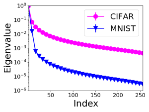
(a) Eigenvalue distributions in each layer for MNIST and CIFAR-10.

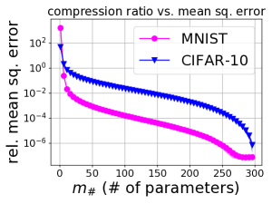
(b) Approximation error with its s.d. versus the width $m^{\sharp}$

Figure 1: Eigenvalue distribution and compression ability of a fully connected network in MNIST and CIFAR-10.

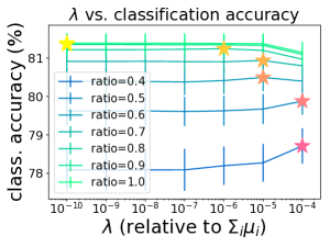
(c) Accuracy versus $\lambda_{\ell}$ in CIFAR-10 for each compression rate.

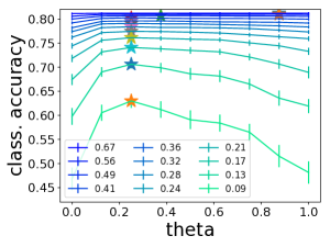
(d) Accuracy versus $\theta$ in CIFAR-10 for each compression rate.

Figure 2: Relation between accuracy and the hyper parameters $\lambda_{\ell}$ and $\theta$. The best $\lambda$ and $\theta$ are indicated by the star symbol.

5 Numerical Experiments

In this section, we conduct numerical experiments to show the validity of our theory and the effectiveness of the proposed method.

5.1 Eigenvalue Distribution and Compression Ability

We show how the rate of decrease in the eigenvalues affects the compression accuracy to justify our theoretical analysis. We constructed a network (namely, NN3) consisting of three hidden fully connected layers with widths $(300,1000,300)$ following the settings in Aghasi et al. (2017) and trained it with 60,000 images in MNIST and 50,000 images in CIFAR-10. Figure 1(a) shows the magnitudes of the eigenvalues of the 3rd hidden layers of the networks trained for each dataset (plotted on a semilog scale). The eigenvalues are sorted in decreasing order, and they are normalized by division by the maximum eigenvalue. We see that eigenvalues for MNIST decrease much more rapidly than those for CIFAR-10. This indicates that MINST is “easier” than CIFAR-10 because the degrees of freedom (an intrinsic dimensionality) of the network trained on MNIST are relatively smaller than those trained on CIFAR-10. Figure 1(b) presents the (relative) compression error $\|\widehat{f}-f^{\sharp}\|_{n}/\|\widehat{f}\|_{n}$ versus the width $m^{\sharp}_{3}$ of the compressed network where we compressed only the 3rd layer and $\lambda_{3}$ was fixed to a constant $10^{-6}\times\mathrm{Tr}[\widehat{\Sigma}_{(\ell)}]$ and $\theta=0.5$. It shows a rapid decrease in the compression error for MNIST than CIFAR-10 (about 100 times smaller). This is because MNIST has faster eigenvalue decay than CIFAR-10.

Figure 1(c) shows the relation between the test classification accuracy and $\lambda_{\ell}$. It is plotted for a VGG-13 network trained on CIFAR-10. We chose the width $m^{\sharp}_{\ell}$ that gave the best accuracy for each $\lambda_{\ell}$ under the constraint of the compression rate (relative number of parameters). We see that as the compression rate increases, the best $\lambda_{\ell}$ goes down. Our theorem tells that $\lambda_{\ell}$ is related to the compression error through (3), that is, as the width goes up, $\lambda_{\ell}$ must goes down. This experiment supports the theoretical evaluation. Figure 1(d) shows the relation between the test classification accuracy and the hyperparameter $\theta$. We can see that the best accuracy is achieved around $\theta=0.3$ for all compression rates, which indicates the superiority of the “combination” of input- and output-information loss and supports our theoretical bound. For low compression rate, the choice of $\lambda_{\ell}$ and $\theta$ does not affect the result so much, which indicates the robustness of the hyper-parameter choice.

5.2 Compression on ImageNet Dataset

We applied our method to the ImageNet (ILSVRC2012) dataset Deng et al. (2009). We compared our method using the ResNet-50 network He et al. (2016) (experiments for VGG-16 network Simonyan and Zisserman (2014) are also shown in Appendix D.1). Our method was compared with the following pruning methods: ThiNet Luo et al. (2017), NISP Yu et al. (2018), and sparse regularization He et al. (2017) (which we call Sparse-reg). As the initial ResNet network, we used two types of networks: ResNet-50-1 and ResNet-50-2. For training ResNet-50-1, we followed the experimental settings in Luo et al. (2017) and Yu et al. (2018). During training, images were resized as in Luo et al. (2017). to 256 $\times$ 256; then, a 224 $\times$ 224 random crop was fed into the network. In the inference stage, we center-cropped the resized images to 224 $\times$ 224. For training ResNet-50-2, we followed the same settings as in He et al. (2017). In particular, images were resized such that the shorter side was 256, and a center crop of 224 $\times$ 224 pixels was used for testing. The augmentation for fine tuning was a 224 $\times$ 224 random crop and its mirror.

We compared ThiNet and NISP for ResNet-50-1 (we call our model for this situation “Spec-ResA”) and Sparse-reg for ResNet-50-2 (we call our model for this situation “Spec-ResB”) for fair comparison. The size of compressed network $f^{\sharp}$ was determined to be as close to the compared network as possible (except, for ResNet-50-2, we did not adopt the “channel sampler” proposed by He et al. (2017) in the first layer of the residual block; hence, our model became slightly larger). The accuracies are borrowed from the scores presented in each paper, and thus we used different models because the original papers of each model reported for each different model. We employed the simultaneous procedure for compression. After pruning, we carried out fine tuning over 10 epochs, where the learning rate was $10^{-3}$ for the first four epochs, $10^{-4}$ for the next four epochs, and $10^{-5}$ for the last two epochs. We employed $\lambda_{\ell}=10^{-6}\times\mathrm{Tr}[\widehat{\Sigma}_{(\ell)}]$ and $\theta=0.5$.

Model	Top-1	Top-5	# Param.	FLOPs
ResNet-50-1	72.89%	91.07%	25.56M	7.75G
ThiNet-70	72.04 %	90.67%	16.94M	4.88G
ThiNet-50	71.01 %	90.02%	12.38M	3.41G
NISP-50-A	72.68%	—	18.63M	5.63G
NISP-50-B	71.99%	—	14.57M	4.32G
Spec-ResA	72.99%	91.56%	12.38M	3.45G
ResNet-50-2	75.21%	92.21%	25.56M	7.75G
Sparse-reg wo/ ft	—	84.2%	19.78M	5.25G
Sparse-reg w/ ft	—	90.8%	19.78M	5.25G
Spec-ResB wo/ ft	66.12%	86.67%	20.69M	5.25G
Spec-ResB w/ ft	74.04%	91.77%	20.69M	5.25G

Table 2: Performance comparison of our method and existing ones for ResNet-50 on ImageNet. “ft” indicates fine tuning after compression.

Table 2 summarizes the performance comparison for ResNet-50. We can see that for both settings, our method outperforms the others for about $1\%$ accuracy. This is an interesting result because ResNet-50 is already compact Luo et al. (2017) and thus there is less room to produce better performance. Moreover, we remark that all layers were simultaneously trained in our method, while other methods were trained one layer after another. Since our method did not adopt the channel sampler proposed by He et al. (2017), our model was a bit larger. However, we could obtain better performance by combining it with our method.

6 Conclusion

In this paper, we proposed a simple pruning algorithm for compressing a network and gave its approximation and generalization error bounds using the degrees of freedom. Unlike the existing compression based generalization error analysis, our analysis is compatible with a practically useful method and further gives a tighter intrinsic dimensionality bound. The proposed algorithm is easily implemented and only requires linear algebraic operations. The numerical experiments showed that the compression ability is related to the eigenvalue distribution, and our algorithm has favorable performance compared to existing methods.

—Appendix—

Appendix A Extension to convolutional neural network

An extension of our method to convolutional layers is a bit tricky. There are several options, but to perform channel-wise pruning, we used the following “covariance matrix” between channels in the experiments. Suppose that a channel $k$ receives the input $\phi_{k;u,v}(x)$ where $1\leq u\leq I_{\tau},~{}1\leq v\leq I_{h}$ indicate the spacial index, then “covariance” between the channels $k$ and $k^{\prime}$ can be formulated as $\widehat{\Sigma}_{k,k^{\prime}}=\frac{1}{n}\sum_{i=1}^{n}(\frac{1}{I_{\tau}I_{h}}\sum_{u,v}\phi_{k;u,v}(x_{i})\phi_{k^{\prime};u,v}(x_{i}))$. As for the covariance between an output channel $k^{\prime}$ and an input channel $k$ (which corresponds to the $(k^{\prime},k)$-th element of $Z^{(\ell)}\widehat{\Sigma}_{F,J}=\mathrm{Cov}(Z^{(\ell)}\phi(X),\phi_{J}(X))$ for the fully connected situation), it can be calculated as $\widehat{\Sigma}_{k^{\prime},k}=\frac{1}{n}\sum_{i=1}^{n}(\frac{1}{I_{\tau}I_{h}}\sum_{u,v}\frac{1}{I^{\prime}_{(u,v)}}\sum_{u^{\prime},v^{\prime}:(u,v)\in\mathrm{Res}(u^{\prime},v^{\prime})}(Z^{(\ell)}\phi(x_{i}))_{k^{\prime};u^{\prime},v^{\prime}}(x_{i})\phi_{k;u,v}(x_{i}))$, where $\mathrm{Res}(u^{\prime},v^{\prime})$ is the receptive field of the location $u^{\prime},v^{\prime}$ in the output channel $k^{\prime}$, and $I^{\prime}_{(u,v)}$ are the number of locations $(u^{\prime},v^{\prime})$ that contain $(u,v)$ in their receptive fields.

Appendix B Proof of Theorem 1

The output of its internal layer (before activation) is denoted by $\hat{F}_{\ell}(x)=(\hat{W}^{(\ell)}\eta(\cdot)+\hat{b}^{(\ell)})\circ\dots\circ(\hat{W}^{(1)}x+\hat{b}^{(1)}).$ We denote the set of row vectors of $Z^{(\ell)}$ by $\mathcal{Z}_{\ell}$, i.e., $\mathcal{Z}_{\ell}=\{Z^{(\ell)\top}_{1,:},\dots,Z^{(\ell)\top}_{m,:}\}$. Conversely, we may define $Z^{(\ell)}$ by specifying ${\mathcal{Z}}_{\ell}$.

Here, we restate Theorem 1 in a complete form that contains both of backward procedure and simultaneous procedure.

Theorem 3 (Restated).

Assume that the regularization parameter $\tau$ in the pruning procedure (2) is defined by the leverage score $\tau\leftarrow\tau^{(\ell)}:=m^{\sharp}_{\ell}\lambda_{\ell}{\tilde{\tau}^{(\ell)}}$.

(i) Backward-procedure: Let $\mathcal{Z}_{\ell}$ for the output information loss be $\mathcal{Z}_{\ell}=\left\{\frac{\sqrt{m_{\ell}q_{j}^{(\ell)}}}{\max_{j^{\prime}}\|\hat{W}^{(\ell)}_{j^{\prime},:}\|}\hat{W}^{(\ell)}_{j,:}\mid j\in J^{\sharp}_{\ell+1}\right\}$ where $q_{j}^{(\ell)}:=\frac{({\tilde{\tau}^{(\ell+1)}}_{j})^{-1}}{\sum_{j^{\prime}\in J^{\sharp}_{\ell+1}}({\tilde{\tau}^{(\ell+1)}}_{j^{\prime}})^{-1}}~{}(j\in J^{\sharp}_{\ell+1})$ and $q_{j}^{(\ell)}=0~{}(\text{otherwise})$, and define $\zeta_{\ell,\theta}=N_{\ell}^{\theta}(\lambda_{\ell})\left(\theta\frac{\max_{j\in[m_{\ell+1}]}\|\hat{W}^{(\ell)}_{j,:}\|^{2}}{\|(\hat{W}^{(\ell)})^{\top}\mathrm{I}_{q^{(\ell)}}\hat{W}^{(\ell)}\|_{\mathrm{op}}}+(1-\theta)m_{\ell}\right)^{-1}$. Then, if we solve the optimization problem (2) with an additional constraint $\sum_{j\in J}({\tilde{\tau}^{(\ell)}}_{j})^{-1}\leq\frac{5}{3}m_{\ell}m^{\sharp}_{\ell}$ for the index set $J$, then the optimization problem is feasible, and the overall approximation error of $f^{\sharp}$ is bounded by

$$\|\widehat{f}-f^{\sharp}\|_{n}\leq\sum\nolimits_{\ell=2}^{L}\left(\bar{R}^{L-\ell+1}\sqrt{{\textstyle\prod_{\ell^{\prime}=\ell}^{L}}\zeta_{\ell^{\prime},\theta}}\right)\sqrt{\lambda_{\ell}},$$ (5)

for $\bar{R}=\sqrt{\hat{c}}R$ where $\hat{c}$ is a universal constant.

(ii) Simultaneous-procedure: Suppose that there exists $c_{\mathrm{scale}}>0$ such that

$$\|\hat{W}^{(\ell)}_{j,:}\|^{2}\leq c_{\mathrm{scale}}R^{2}{\tilde{\tau}^{(\ell+1)}}_{j},$$ (6)

and we employ ${\mathcal{Z}}_{\ell}=\{\hat{W}^{(\ell)}_{j,:}/\|\hat{W}^{(\ell)}_{j,:}\|\mid j\in[m_{\ell+1}]\}$ for the output aware objective. Then, we have the same bound as (5) for $q_{j}^{(\ell)}=({\tilde{\tau}^{(\ell+1)}}_{j})^{-1}/\sum_{j^{\prime}\in[m_{\ell+1}]}({\tilde{\tau}^{(\ell+1)}}_{j^{\prime}})^{-1}~{}(\forall j\in[m_{\ell+1}])$ and

$$\zeta_{\ell,\theta}=c_{\mathrm{scale}}N_{\ell}^{\theta}(\lambda_{\ell})\left(\theta{\textstyle\frac{m^{\sharp}_{\ell+1}\max_{j}q_{j}^{(\ell)}\|\hat{W}^{(\ell)}_{j,:}\|^{2}}{\|(\hat{W}^{(\ell)})^{\top}\mathrm{I}_{q^{(\ell)}}\hat{W}^{(\ell)}\|_{\mathrm{op}}}}+(1-\theta)m^{\sharp}_{\ell+1}\right)^{-1}.$$ (7)

The assumption (6) is rather strong, but we see that it is always satisfied by $c_{\mathrm{scale}}=1$ when $\lambda_{\ell}=0$ and by $c_{\mathrm{scale}}=\mathrm{Tr}[\widehat{\Sigma}_{(\ell+1)}]/(m_{\ell+1}\min_{j}\widehat{\Sigma}_{(\ell+1),(j,j)})$ when $\lambda_{\ell}=\infty$. Thus, it is satisfied if the variances of the nodes in the $\ell+1$-th layer is balanced, which is ensured if we are applying batch normalization.

B.1 Preparation of lemmas

To derive the approximation error bound. we utilize the following proposition that was essentially proven by Bach (2017). This proposition states the connection between the degrees of freedom and the compression error, that is, it characterize the sufficient width $m^{\sharp}_{\ell}$ to obtain a pre-specified compression error $\lambda_{\ell}$. Actually, we will see that the eigenvalue essentially controls this relation through the degrees of freedom.

Proposition 1.

There exists a probability measure $q_{\ell}$ on $\{1,\dots,m_{\ell}\}$ such that for any $\delta\in(0,1)$ and $\lambda>0$, i.i.d. sample $v_{1},\dots,v_{m}\in\{1,\dots,m_{\ell}\}$ from $q_{\ell}$ satisfies, with probability $1-\delta$, that

$$\inf_{\beta\in\mathbb{R}^{m}}\left\{\left\|\alpha^{\top}\eta(\hat{F}_{\ell-1}(\cdot))-\sum_{j=1}^{m}\beta_{j}q_{\ell}(v_{j})^{-1/2}\eta(\hat{F}_{\ell-1}(\cdot))_{v_{j}}\right\|_{n}^{2}+m\lambda\|\beta\|^{2}\right\}$$

$$\leq 4\lambda\alpha^{\top}\widehat{\Sigma}_{\ell}(\widehat{\Sigma}_{\ell}+\lambda\mathrm{I})^{-1}\alpha,$$

for every $\alpha\in\mathbb{R}^{m_{\ell}}$, if

$$m\geq 5\hat{N}_{\ell}(\lambda)\log(16\hat{N}_{\ell}(\lambda)/\delta).$$

Moreover, the optimal solution $\hat{\beta}$ satisfies $\|\hat{\beta}\|_{2}^{2}\leq\frac{4\|\alpha\|^{2}}{m}$.

Proof.

This is basically a direct consequence from Proposition 1 in Bach (2017) and its discussions. The original statement does not include the regularization term $m\lambda\|\beta\|^{2}$ in the LHS and $\alpha^{\top}\widehat{\Sigma}_{\ell}(\widehat{\Sigma}_{\ell}+\lambda\mathrm{I})^{-1}\alpha$ in the right hand side. However, by carefully following the proof, the bound including these additional factors is indeed proven.

The norm bond of $\hat{\beta}$ is guaranteed by the following relation:

$$m\lambda\|\hat{\beta}\|^{2}\leq 4\lambda\alpha^{\top}\widehat{\Sigma}_{\ell}(\widehat{\Sigma}_{\ell}+\lambda\mathrm{I})^{-1}\alpha\leq 4\lambda\|\alpha\|^{2}.$$

∎

Proposition 1 indicates the following lemma by the the scale invariance of $\eta$, $\eta(ax)=a\eta(x)~{}(a>0)$.

Lemma 1.

Suppose that

$$\tau^{\prime}_{j}=\frac{1}{\hat{N}_{\ell}(\lambda)}\sum_{l=1}^{m_{\ell}}U_{j,l}^{2}\frac{\hat{\mu}_{l}^{(\ell)}}{\hat{\mu}_{l}^{(\ell)}+\lambda}=\frac{1}{\hat{N}_{\ell}(\lambda)}[\widehat{\Sigma}^{(\ell)}(\widehat{\Sigma}^{(\ell)}+\lambda\mathrm{I})^{-1}]_{j,j}~{}~{}(j\in\{1,\dots,m_{\ell}\}),$$ (8)

where $U=(U_{j,l})_{j,l}$ is the orthogonal matrix that diagonalizes $\widehat{\Sigma}^{(\ell)}$, that is, $\widehat{\Sigma}^{(\ell)}=U\mathrm{diag}\left(\hat{\mu}_{1}^{(\ell)},\dots,\hat{\mu}_{m_{\ell}}^{(\ell)}\right)U^{\top}$. For $\lambda>0$, and any $1/2>\delta>0$, if

$$m\geq 5\hat{N}_{\ell}(\lambda)\log(16\hat{N}_{\ell}(\lambda)/\delta),$$

then there exist $v_{1},\dots,v_{m}\in\{1,\dots,m_{\ell}\}$ such that, for every $\alpha\in\mathbb{R}^{m_{\ell}}$,

$$\inf_{\beta\in\mathbb{R}^{m}}\left\{\left\|\alpha^{\top}\eta(\hat{F}_{\ell-1}(\cdot))-\sum_{j=1}^{m}\beta_{j}{\tau^{\prime}_{j}}^{-1/2}\eta(\hat{F}_{\ell-1}(\cdot))_{v_{j}}\right\|_{n}^{2}+m\lambda\|\beta\|^{2}\right\}$$

$$\leq 4\lambda\alpha^{\top}\widehat{\Sigma}^{(\ell)}(\widehat{\Sigma}^{(\ell)}+\lambda\mathrm{I})^{-1}\alpha,$$ (9)

and

$$\sum_{j=1}^{m}{\tau_{j}^{\prime}}^{-1}\leq(1-2\delta)^{-1}m\times m_{\ell}.$$

Proof.

Suppose that the measure $Q_{\ell}$ is the counting measure, $Q_{\ell}(J)=|J|$ for $J\subset\{1,\dots,m_{\ell}\}$, and $q_{\ell}$ is a density given by $q_{\ell}(j)=\tau^{\prime}_{j}~{}(j\in\{1,\dots,m_{\ell}\})$ with respect to the base measure $Q_{\ell}$. Suppose that $v_{1},\dots,v_{m}\in\{1,\dots,m_{\ell}\}$ is an i.i.d. sequence distributed from $q_{\ell}\mathrm{d}Q_{\ell}$, then Bach (2017) showed that this sequence satisfies the assertion given in Proposition 1.

Notice that $\mathrm{E}_{v}[\frac{1}{m}\sum_{j=1}^{m}q_{\ell}(v_{j})^{-1}]=\mathrm{E}_{v}[q_{\ell}(v)^{-1}]=\int_{[m_{\ell}]}q_{\ell}(v)^{-1}q_{\ell}(v)\mathrm{d}Q_{\ell}(v)=\int_{[m_{\ell}]}1\mathrm{d}Q_{\ell}(v)=m_{\ell}$, thus an i.i.d. sequence $\{v_{1},\dots,v_{m}\}$ satisfies $\frac{1}{m}\sum_{j=1}^{m}q_{\ell}(v_{j})^{-1}\leq m_{\ell}/(1-2\delta)$ with probability $2\delta$ by the Markov’s inequality. Combining this with Proposition 1, the i.i.d. sequence $\{v_{1},\dots,v_{m}\}$ and $\tau^{\prime}_{j}=q_{\ell}(v_{j})$ satisfies the condition in the statement with probability $1-(\delta+1-2\delta)=\delta>0$. This ensures the existence of sequences $\{v_{j}\}_{j=1}^{m}$ and $\{\tau^{\prime}_{j}\}_{j=1}^{m}$ that satisfy the assertion. ∎

B.2 Proof of Theorem 1

B.2.1 General fact

Since Lemma 1 with $\delta=1/5$ states that if $m^{\sharp}_{\ell}\geq 5\hat{N}_{\ell}(\lambda_{\ell})\log(80\hat{N}_{\ell}(\lambda_{\ell}))$, then there exists $J\subset[m_{\ell}]^{m^{\sharp}_{\ell}}$ such that

$$\inf_{\alpha\in\mathbb{R}^{|J|}}\|z^{\top}\phi-\alpha^{\top}\phi_{J}\|_{n}^{2}+\lambda_{\ell}|J|\|\alpha\|_{\tau^{\prime}}^{2}\leq 4\lambda_{\ell}z^{\top}\widehat{\Sigma}_{\ell}(\widehat{\Sigma}_{\ell}+\lambda\mathrm{I})^{-1}z~{}~{}~{}(\forall z\in\mathbb{R}^{m_{\ell}}),$$

and

$$\sum_{j\in J^{\sharp}_{\ell}}({\tilde{\tau}^{(\ell)}}_{j})^{-1}\leq\frac{5}{3}m_{\ell}\times m^{\sharp}_{\ell}$$ (10)

is satisfied (here, note that $\tau^{\prime}$ given in Eq. (8) is equivalent to ${\tilde{\tau}^{(\ell)}}$).

Evaluation of $L^{(\mathrm{A})}_{\tau}(J)$: By setting $z=e_{j}~{}(j=1,\dots,m_{\ell})$ where $e_{j}$ is an indicator vector which has $1$ at its $j$-th component and $0$ in other components, and summing up them for $j=1,\dots,m_{\ell}$, it holds that

$$L^{(\mathrm{A})}_{\tau}(J)=\inf_{A\in\mathbb{R}^{m_{\ell}\times|J|}}\|\phi-A\phi_{J}\|_{n}^{2}+\lambda_{\ell}|J|\|A\|_{\tau^{\prime}}^{2}\leq 4\lambda_{\ell}\hat{N}_{\ell}(\lambda_{\ell}),$$

for the same $J$ as above. Here, the optimal $A$, which is denoted by $\hat{A}_{J}$, is given by

$$\hat{A}_{J}=\widehat{\Sigma}_{F,J}(\widehat{\Sigma}_{J,J}+\mathrm{I}_{\tau})^{-1}.$$

Evaluation of $L^{(\mathrm{B})}_{\tau}(J)$: By letting $z\in\mathcal{Z}_{\ell}$ and summing up them, we also have

$$L^{(\mathrm{B})}_{\tau}(J)=\inf_{B\in\mathbb{R}^{m^{\sharp}_{\ell+1}\times|J|}}\|Z^{(\ell)}\phi-B\phi_{J}\|_{n}^{2}+\lambda_{\ell}|J|\|B\|_{\tau^{\prime}}^{2}\leq 4\lambda_{\ell}\mathrm{Tr}[Z^{(\ell)}\widehat{\Sigma}_{\ell}(\widehat{\Sigma}_{\ell}+\lambda_{\ell}\mathrm{I})^{-1}Z^{(\ell)\top}].$$

for the same $J$ as above. Remind again that the optimal $B$, which is denoted by $\hat{B}_{J}$, is given by

$$\hat{B}_{J}=Z^{(\ell)}\widehat{\Sigma}_{F,J}(\widehat{\Sigma}_{J,J}+\mathrm{I}_{\tau})^{-1}=Z^{(\ell)}\hat{A}_{J}.$$

Combining the bounds for $L^{(\mathrm{A})}_{\tau}(J)$ and $L^{(\mathrm{B})}_{\tau}(J)$: By combining the above evaluation, we have that

$$\theta L^{(\mathrm{A})}_{\tau}(J^{\sharp})+(1-\theta)L^{(\mathrm{B})}_{\tau}(J^{\sharp})\leq 4\lambda_{\ell}\{\theta\hat{N}_{\ell}(\lambda_{\ell})+(1-\theta)\mathrm{Tr}[Z^{(\ell)}\widehat{\Sigma}^{(\ell)}(\widehat{\Sigma}^{(\ell)}+\lambda_{\ell}\mathrm{I})^{-1}Z^{(\ell)\top}]\},$$

where $J^{\sharp}_{\ell}$ is the minimizer of $\theta L^{(\mathrm{A})}_{\tau}(J)+(1-\theta)L^{(\mathrm{B})}_{\tau}(J)$ with respect to $J$.

From now on, we let $\tau=\lambda_{\ell}m^{\sharp}_{\ell}\tau^{\prime}(=\lambda_{\ell}|J^{\sharp}_{\ell}|\tau^{\prime})$ as defined in the main text.

B.2.2 (i) Backward-procedure

From now on, we give the bound corresponding to the backward-procedure. The proof consists of three parts: (i) evaluation of the compression error in each layer, (ii) evaluation of the norm of the weight matrix for the compressed network, and (iii) overall compression error of whole layer. In (i), we use Lemma 1 to evaluate the compression error based on the eigenvalue distribution of the covariance matrix. In (ii), we again use Lemma 1 to bound the norm of the compressed network. This is important to evaluate the overall compression error because the norm controls how the compression error in each layer propagates to the final output. In (iii), we combine the results in (i) and (ii) to obtain the overall compression error.

First, note that, for the choice of ${\mathcal{Z}}_{\ell}=\left\{\frac{\sqrt{m_{\ell}q_{j}^{(\ell)}}}{\max_{j^{\prime}}\|\hat{W}^{(\ell)}_{j^{\prime},:}\|}\hat{W}^{(\ell)}_{j,:}\mid j\in J^{\sharp}_{\ell+1}\right\}$, it holds that

$$L^{(\mathrm{B})}_{\tau}(J^{\sharp}_{\ell})\leq 4\lambda_{\ell}\sum_{z\in{\mathcal{Z}}_{\ell}}z^{\top}\widehat{\Sigma}_{\ell}(\widehat{\Sigma}_{\ell}+\lambda_{\ell}\mathrm{I})^{-1}z\leq 4\lambda_{\ell}\sum_{z\in{\mathcal{Z}}_{\ell}}\|z\|^{2}\leq 4\lambda_{\ell}m_{\ell}\sum_{j\in J^{\sharp}_{\ell+1}}q_{j}^{(\ell)}=4\lambda_{\ell}m_{\ell}.$$

Compression error bound: Here, we give the compression error bound of the backward procedure. For the optimal $J^{\sharp}_{\ell}$, we have that

$$\inf_{\alpha\in\mathbb{R}^{|J^{\sharp}_{\ell}|}}\|\hat{W}^{(\ell)}_{j,:}\phi-\alpha^{\top}\phi_{J^{\sharp}}\|_{n}^{2}+\|\alpha\|_{\tau}^{2} =\hat{W}^{(\ell)}_{j,:}[\widehat{\Sigma}_{F,F}-\widehat{\Sigma}_{F,J^{\sharp}}(\widehat{\Sigma}_{J^{\sharp},J^{\sharp}}+\mathrm{I}_{\tau})^{-1}\widehat{\Sigma}_{J^{\sharp},F}](\hat{W}^{(\ell)}_{j,:})^{\top}$$

$$=\mathrm{Tr}\{[\widehat{\Sigma}_{F,F}-\widehat{\Sigma}_{F,J^{\sharp}}(\widehat{\Sigma}_{J^{\sharp},J^{\sharp}}+\mathrm{I}_{\tau})^{-1}\widehat{\Sigma}_{J^{\sharp},F}](\hat{W}^{(\ell)}_{j,:})^{\top}\hat{W}^{(\ell)}_{j,:}\},$$

and the optimal $\alpha$ in the left hand side is given by $\hat{W}^{(\ell)}_{j,:}\hat{A}_{J^{\sharp}_{\ell}}$. Hence, it holds that

$$\sum_{j\in J^{\sharp}_{\ell+1}}\inf_{\alpha\in\mathbb{R}^{|J^{\sharp}_{\ell}|}}\left\{\|{q_{j}^{(\ell)}}^{1/2}\hat{W}^{(\ell)}_{j,:}\phi-\alpha^{\top}\phi_{J^{\sharp}_{\ell}}\|_{n}^{2}+\|\alpha\|_{\tau}^{2}\right\}=\sum_{j\in J^{\sharp}_{\ell+1}}{q_{j}^{(\ell)}}\inf_{\alpha\in\mathbb{R}^{|J^{\sharp}_{\ell}|}}\left\{\|\hat{W}^{(\ell)}_{j,:}\phi-\alpha^{\top}\phi_{J^{\sharp}_{\ell}}\|_{n}^{2}+\|\alpha\|_{\tau}^{2}\right\}$$

$$=\sum_{j\in J^{\sharp}_{\ell+1}}{q_{j}^{(\ell)}}\mathrm{Tr}\{[\widehat{\Sigma}_{F,F}-\widehat{\Sigma}_{F,J^{\sharp}_{\ell}}(\widehat{\Sigma}_{J^{\sharp}_{\ell},J^{\sharp}_{\ell}}+\mathrm{I}_{\tau})^{-1}\widehat{\Sigma}_{J^{\sharp}_{\ell},F}](\hat{W}^{(\ell)}_{j,:})^{\top}\hat{W}^{(\ell)}_{j,:}\}$$

$$=\mathrm{Tr}\{[\widehat{\Sigma}_{F,F}-\widehat{\Sigma}_{F,J^{\sharp}_{\ell}}(\widehat{\Sigma}_{J^{\sharp}_{\ell},J^{\sharp}_{\ell}}+\mathrm{I}_{\tau})^{-1}\widehat{\Sigma}_{J^{\sharp}_{\ell},F}](\hat{W}^{(\ell)})^{\top}\mathrm{I}_{q^{(\ell)}}\hat{W}^{(\ell)}\}$$

$$\leq\mathrm{Tr}[\widehat{\Sigma}_{F,F}-\widehat{\Sigma}_{F,J^{\sharp}_{\ell}}(\widehat{\Sigma}_{J^{\sharp}_{\ell},J^{\sharp}_{\ell}}+\mathrm{I}_{\tau})^{-1}\widehat{\Sigma}_{J^{\sharp}_{\ell},F}]\|(\hat{W}^{(\ell)})^{\top}\mathrm{I}_{q^{(\ell)}}\hat{W}^{(\ell)}\|_{\mathrm{op}}$$

$$=L^{(\mathrm{A})}_{\tau}(J^{\sharp}_{\ell})\|(\hat{W}^{(\ell)})^{\top}\mathrm{I}_{q^{(\ell)}}\hat{W}^{(\ell)}\|_{\mathrm{op}}\leq L^{(\mathrm{A})}_{\tau}(J^{\sharp}_{\ell})\frac{\|(\hat{W}^{(\ell)})^{\top}\mathrm{I}_{q^{(\ell)}}\hat{W}^{(\ell)}\|_{\mathrm{op}}}{\max_{j\in[m_{\ell+1}]}\|\hat{W}^{(\ell)}_{j,:}\|^{2}}\max_{j\in[m_{\ell+1}]}\|\hat{W}^{(\ell)}_{j,:}\|^{2}$$

$$\leq L^{(\mathrm{A})}_{\tau}(J^{\sharp}_{\ell})\frac{m_{\ell}\|(\hat{W}^{(\ell)})^{\top}\mathrm{I}_{q^{(\ell)}}\hat{W}^{(\ell)}\|_{\mathrm{op}}}{\max_{j\in[m_{\ell+1}]}\|\hat{W}^{(\ell)}_{j,:}\|^{2}}\frac{R^{2}}{m_{\ell+1}m_{\ell}},$$

where where we used the assumption $\max_{j}\|W^{(\ell)}_{j,:}\|\leq R/\sqrt{m_{\ell+1}}$. In the same manner, we also have that

$$\sum_{j\in J^{\sharp}_{\ell+1}}{q_{j}^{(\ell)}}\inf_{\alpha\in\mathbb{R}^{|J^{\sharp}_{\ell}|}}\left\{\|\hat{W}^{(\ell)}_{j,:}\phi-\alpha^{\top}\phi_{J^{\sharp}_{\ell}}\|_{n}^{2}+\|\alpha\|_{\tau}^{2}\right\}$$

$$=\frac{\max_{j^{\prime}}\|\hat{W}^{(\ell)}_{j^{\prime},:}\|^{2}}{m_{\ell}}\sum_{j\in{J^{\sharp}_{\ell+1}}}\inf_{\alpha\in\mathbb{R}^{|J^{\sharp}_{\ell}|}}\left\|{\textstyle\frac{\sqrt{m_{\ell}q_{j}^{(\ell)}}}{\max_{j^{\prime}}\|\hat{W}^{(\ell)}_{j^{\prime},:}\|}}\hat{W}^{(\ell)}_{j,:}\phi-\alpha^{\top}\phi_{J^{\sharp}_{\ell}}\right\|_{n}^{2}+\|\alpha\|_{\tau}^{2}=$$

$$\leq L^{(\mathrm{B})}_{\tau}(J^{\sharp}_{\ell})\frac{\max_{j\in[m_{\ell+1}]}\|\hat{W}^{(\ell)}_{j,:}\|^{2}}{m_{\ell}}\leq L^{(\mathrm{B})}_{\tau}(J^{\sharp}_{\ell})\frac{R^{2}}{m_{\ell}m_{\ell+1}}.$$

These inequalities imply that

$$\sum_{j\in J^{\sharp}_{\ell+1}}q_{j}^{(\ell)}\left\{\|\hat{W}^{(\ell)}_{j,:}\phi-\hat{W}^{(\ell)}_{j,:}\hat{A}_{J^{\sharp}}\phi_{J^{\sharp}}\|_{n}^{2}+\|\hat{W}^{(\ell)}_{j,:}\hat{A}_{J^{\sharp}}\|_{\tau}^{2}\right\}$$

$$\leq 4\lambda_{\ell}\frac{\{\theta\hat{N}_{\ell}(\lambda_{\ell})+(1-\theta)\mathrm{Tr}[Z^{(\ell)}\widehat{\Sigma}_{\ell}(\widehat{\Sigma}_{\ell}+\lambda_{\ell}\mathrm{I})^{-1}Z^{(\ell)\top}]\}}{\theta\frac{\max_{j\in[m_{\ell+1}]}\|\hat{W}^{(\ell)}_{j,:}\|^{2}}{m_{\ell}\|(\hat{W}^{(\ell)})^{\top}\mathrm{I}_{q^{(\ell)}}\hat{W}^{(\ell)}\|_{\mathrm{op}}}+(1-\theta)}\frac{R^{2}}{m_{\ell}m_{\ell+1}}$$

$$\leq 4\lambda_{\ell}\frac{\{\theta\hat{N}_{\ell}(\lambda_{\ell})+(1-\theta)m_{\ell}\}}{\left[\theta\frac{\max_{j\in[m_{\ell+1}]}\|\hat{W}^{(\ell)}_{j,:}\|^{2}}{m_{\ell}\|(\hat{W}^{(\ell)})^{\top}\mathrm{I}_{q^{(\ell)}}\hat{W}^{(\ell)}\|_{\mathrm{op}}}+(1-\theta)\right]m_{\ell}}\frac{R^{2}}{m_{\ell+1}}$$

$$\leq 4\lambda_{\ell}\zeta_{\ell,\theta}\frac{R^{2}}{m_{\ell+1}}.$$ (11)

Norm bound of the coefficients: Here, we give an upper bound of the norm of the weight matrices for the compressed network. From (11) and the definition that $\tau^{(\ell)}=\lambda_{\ell}m^{\sharp}_{\ell}{\tilde{\tau}^{(\ell)}}$, we have that

$$\sum_{j\in J^{\sharp}_{\ell+1}}q_{j}^{(\ell)}\|\hat{W}^{(\ell)}_{j,:}\hat{A}_{J^{\sharp}}\|_{{\tilde{\tau}^{(\ell)}}}^{2}\leq\frac{1}{\lambda_{\ell}m^{\sharp}_{\ell}}4\lambda_{\ell}\zeta_{\ell,\theta}\frac{R^{2}}{m_{\ell+1}}=4\zeta_{\ell,\theta}\frac{R^{2}}{m_{\ell+1}m^{\sharp}_{\ell}}.$$

Here, by Eq. (10), the condition $\sum_{j\in J^{\sharp}_{\ell+1}}({\tilde{\tau}^{(\ell+1)}}_{j})^{-1}\leq\frac{5}{3}m_{\ell+1}m^{\sharp}_{\ell+1}$ is feasible, and under this condition, we also have that

$$\sum_{j\in J^{\sharp}_{\ell+1}}({\tilde{\tau}^{(\ell+1)}}_{j})^{-1}\|\hat{W}^{(\ell)}_{j,:}\hat{A}_{J^{\sharp}}\|_{{\tilde{\tau}^{(\ell)}}}^{2}\leq 4\zeta_{\ell,\theta}\frac{R^{2}}{m_{\ell+1}m^{\sharp}_{\ell}}\times\frac{5}{3}m_{\ell+1}m^{\sharp}_{\ell+1}=\frac{20}{3}\zeta_{\ell,\theta}\frac{m^{\sharp}_{\ell+1}}{m^{\sharp}_{\ell}}R^{2},$$

where we used the definition $q$ Similarly, the approximation error bound Eq. (11) can be rewritten as

$$\sum_{j\in J^{\sharp}_{\ell+1}}({\tilde{\tau}^{(\ell+1)}}_{j})^{-1}\|\hat{W}^{(\ell)}_{j,:}\phi-\hat{W}^{(\ell)}_{j,:}\hat{A}_{J^{\sharp}}\phi_{J^{\sharp}}\|_{n}^{2}\leq\frac{20}{3}\lambda_{\ell}\zeta_{\ell,\theta}m^{\sharp}_{\ell+1}R^{2}.$$ (12)

For $\ell=L$, the same inequality holds for $m_{L+1}=m^{\sharp}_{L+1}=1$ and ${\tilde{\tau}^{(L+1)}}_{j}=1~{}(j=1)$.

Overall approximation error bound: Given these inequalities, we bound the overall approximation error bound. Let $J^{\sharp}_{\ell}$ be the optimal index set chosen by Spectral Pruning for the $\ell$-th layer, and the parameters of compressed network be denoted by

$$W^{\sharp(\ell)}=\hat{W}^{(\ell)}_{J^{\sharp}_{\ell+1},[m_{\ell}]}\hat{A}_{J^{\sharp}_{\ell}}\in\mathbb{R}^{m^{\sharp}_{\ell+1}\times m^{\sharp}_{\ell}},~{}~{}b^{\sharp(\ell)}=\hat{b}^{(\ell)}_{J^{\sharp}_{\ell+1}}\in\mathbb{R}^{m^{\sharp}_{\ell+1}}.$$

Then, it holds that

$$f^{\sharp}(x) =(W^{\sharp(L)}\eta(\cdot)+b^{\sharp(L)})\circ\dots\circ(W^{\sharp(1)}x+b^{\sharp(1)}).$$

Then, due to the scale invariance of $\eta$, we also have

$$f^{\sharp}(x) =(W^{\sharp(L)}\mathrm{I}_{({\tilde{\tau}^{(L)}})^{\frac{1}{2}}}\eta(\cdot)+b^{\sharp(L)})\circ(\mathrm{I}_{({\tilde{\tau}^{(L)}})^{-\frac{1}{2}}}W^{\sharp(L-1)}\mathrm{I}_{({\tilde{\tau}^{(L-1)}})^{\frac{1}{2}}}\eta(\cdot)+\mathrm{I}_{({\tilde{\tau}^{(L)}})^{-\frac{1}{2}}}b^{\sharp(L-1)})\dots\circ(\mathrm{I}_{({\tilde{\tau}^{(2)}})^{-\frac{1}{2}}}W^{\sharp(1)}x+\mathrm{I}_{({\tilde{\tau}^{(2)}})^{-\frac{1}{2}}}b^{\sharp(1)}).$$

Then, if we define as $\widetilde{W}^{(\ell)}=\mathrm{I}_{({\tilde{\tau}^{(\ell+1)}})^{-\frac{1}{2}}}W^{\sharp(\ell)}\mathrm{I}_{({\tilde{\tau}^{(\ell)}})^{\frac{1}{2}}}$ and $\tilde{b}^{(\ell)}=\mathrm{I}_{({\tilde{\tau}^{(\ell+1)}})^{-\frac{1}{2}}}b^{\sharp(\ell)}$, then we also have another representation of $f^{\sharp}$ as

$$f^{\sharp}(x) =(\widetilde{W}^{(L)}\eta(\cdot)+\tilde{b}^{(L)})\circ\dots\circ(\widetilde{W}^{(1)}x+\tilde{b}^{(1)}).$$

In the same manner, the original trained network $\widehat{f}$ is also rewritten as

$$\widehat{f}(x) =(\hat{W}^{(L)}\eta(\cdot)+\hat{b}^{(L)})\circ\dots\circ(\hat{W}^{(1)}x+\hat{b}^{(1)})$$

$$=(\hat{W}^{(L)}\mathrm{I}_{({\tilde{\tau}^{(L)}})^{\frac{1}{2}}}\eta(\cdot)+\hat{b}^{(L)})\circ(\mathrm{I}_{({\tilde{\tau}^{(L)}})^{-\frac{1}{2}}}\hat{W}^{(L-1)}\mathrm{I}_{({\tilde{\tau}^{(L-1)}})^{\frac{1}{2}}}\eta(\cdot)+\mathrm{I}_{({\tilde{\tau}^{(L)}})^{-\frac{1}{2}}}\hat{b}^{(L-1)})\circ\dots\circ(\mathrm{I}_{({\tilde{\tau}^{(2)}})^{-\frac{1}{2}}}\hat{W}^{(1)}x+\mathrm{I}_{({\tilde{\tau}^{(2)}})^{-\frac{1}{2}}}\hat{b}^{(1)})$$

$$=:(\ddot{W}^{(L)}\eta(\cdot)+\ddot{b}^{(L)})\circ\dots\circ(\ddot{W}^{(1)}x+\ddot{b}^{(1)}),$$

where we defined $\ddot{W}^{(\ell)}:=\mathrm{I}_{({\tilde{\tau}^{(\ell+1)}})^{-\frac{1}{2}}}\hat{W}^{(\ell)}\mathrm{I}_{({\tilde{\tau}^{(\ell)}})^{\frac{1}{2}}}$ and $\ddot{b}^{(\ell)}:=\mathrm{I}_{({\tilde{\tau}^{(\ell+1)}})^{-\frac{1}{2}}}\hat{b}^{(\ell)}$.

Then, the difference between $f^{\sharp}$ and $\widehat{f}$ can be decomposed into

$$f^{\sharp}(x)-\widehat{f}(x)=(\widetilde{W}^{(L)}\eta(\cdot)+\tilde{b}^{(L)})\circ\dots\circ(\widetilde{W}^{(1)}x+\tilde{b}^{(1)})-(\ddot{W}^{(L)}\eta(\cdot)+\ddot{b}^{(L)})\circ\dots\circ(\ddot{W}^{(1)}x+\ddot{b}^{(1)})$$

$$= \sum_{\ell=2}^{L}\Big{\{}(\widetilde{W}^{(L)}\eta(\cdot)+\tilde{b}^{(L)})\circ\dots\circ(\widetilde{W}^{(\ell+1)}\eta(\cdot)+\tilde{b}^{(\ell+1)})\circ(\widetilde{W}^{(\ell)}\eta(\cdot)+\tilde{b}^{(\ell)})\circ(\ddot{W}^{(\ell-1)}\eta(\cdot)+\ddot{b}^{(\ell-1)})\circ\dots\circ(\ddot{W}^{(1)}x+\ddot{b}^{(1)})$$

$$-(\widetilde{W}^{(L)}\eta(\cdot)+\tilde{b}^{(L)})\circ\dots\circ(\widetilde{W}^{(\ell+1)}\eta(\cdot)+\tilde{b}^{(\ell+1)})\circ(\ddot{W}^{(\ell)}\eta(\cdot)+\ddot{b}^{(\ell)})\circ(\ddot{W}^{(\ell-1)}\eta(\cdot)+\ddot{b}^{(\ell-1)})\circ\dots\circ(\ddot{W}^{(1)}x+\ddot{b}^{(1)})\Big{\}}.$$

We evaluate the $\|\cdot\|_{n}$-norm of this difference. First, notice that Eq. (12) is equivalent to the following inequality:

$$\|(\widetilde{W}^{(\ell)}\eta(\cdot)+\tilde{b}^{(\ell)})\circ(\ddot{W}^{(\ell-1)}\eta(\cdot)+\ddot{b}^{(\ell-1)})\circ\dots\circ(\ddot{W}^{(1)}\cdot+\ddot{b}^{(1)})$$

$$-(\ddot{W}^{(\ell)}_{J^{\sharp}_{\ell+1},[m_{\ell}]}\eta(\cdot)+\ddot{b}^{(\ell)})\circ(\ddot{W}^{(\ell-1)}\eta(\cdot)+\ddot{b}^{(\ell-1)})\circ\dots\circ(\ddot{W}^{(1)}\cdot+\ddot{b}^{(1)})\|_{n}^{2}\leq\hat{c}\lambda_{\ell}\zeta_{\ell,\theta}m^{\sharp}_{\ell+1}R^{2}.$$

(We can check that, even for $\ell=2$, this inequality is correct.) Next, by evaluating the Lipschitz continuity of the $\ell$-th layer of $f^{\sharp}$ as

$$\|\widetilde{W}^{(\ell)}g-\widetilde{W}^{(\ell)}g^{\prime}\|_{n}^{2} =\frac{1}{n}\sum_{i=1}^{n}\|\widetilde{W}^{(\ell)}g(x_{i})-\widetilde{W}^{(\ell)}g^{\prime}(x_{i})\|^{2}$$

$$=\frac{1}{n}\sum_{i=1}^{n}(g(x_{i})-g^{\prime}(x_{i}))^{\top}(\widetilde{W}^{(\ell)})^{\top}\widetilde{W}^{(\ell)}(g(x_{i})-g^{\prime}(x_{i}))$$

$$\leq\frac{1}{n}\sum_{i=1}^{n}\|g(x_{i})-g^{\prime}(x_{i})\|^{2}\mathrm{Tr}[(\widetilde{W}^{(\ell)})^{\top}\widetilde{W}^{(\ell)}]$$

$$\leq\hat{c}\zeta_{\ell,\theta}\frac{m^{\sharp}_{\ell+1}}{m^{\sharp}_{\ell}}R^{2}\|g-g^{\prime}\|_{n}^{2},$$

for $g,g^{\prime}:\mathbb{R}^{d}\to\mathbb{R}^{m^{\sharp}_{\ell}}$, then it holds that

$$\|(\widetilde{W}^{(L)}\eta(\cdot)+\tilde{b}^{(L)})\circ\dots\circ(\widetilde{W}^{(\ell+1)}\eta(\cdot)+\tilde{b}^{(\ell+1)})\circ(\widetilde{W}^{(\ell)}\eta(\cdot)+\tilde{b}^{(\ell)})\circ(\ddot{W}^{(\ell-1)}\eta(\cdot)+\ddot{b}^{(\ell-1)})\circ\dots\circ(\ddot{W}^{(1)}x+\ddot{b}^{(1)})$$

$$-(\widetilde{W}^{(L)}\eta(\cdot)+\tilde{b}^{(L)})\circ\dots\circ(\widetilde{W}^{(\ell+1)}\eta(\cdot)+\tilde{b}^{(\ell+1)})\circ(\ddot{W}^{(\ell)}\eta(\cdot)+\ddot{b}^{(\ell)})\circ(\ddot{W}^{(\ell-1)}\eta(\cdot)+\ddot{b}^{(\ell-1)})\circ\dots\circ(\ddot{W}^{(1)}x+\ddot{b}^{(1)})\|_{n}^{2}$$

$$\leq \prod_{\ell^{\prime}=\ell+1}^{L}\hat{c}\zeta_{\ell^{\prime},\theta}\frac{m^{\sharp}_{\ell^{\prime}+1}}{m^{\sharp}_{\ell^{\prime}}}R^{2}\cdot\hat{c}\lambda_{\ell}\zeta_{\ell,\theta}m^{\sharp}_{\ell+1}R^{2}\leq\lambda_{\ell}\prod_{\ell^{\prime}=\ell}^{L}(\hat{c}\zeta_{\ell^{\prime},\theta}R^{2})=\lambda_{\ell}\bar{R}^{2(L-\ell+1)}\prod_{\ell^{\prime}=\ell}^{L}\zeta_{\ell^{\prime},\theta}.$$

Then, by summing up the square root of this for $\ell=2,\dots,L$, then we have the whole approximation error bound.

B.2.3 Simultaneous procedure

Here, we give bounds corresponding to the simultaneous-procedure. The proof techniques are quite similar to the forward procedure. However, instead of the $\ell_{2}$-norm bound derived in the backward-procedure, we derive $\ell_{\infty}$-norm bound for both of the approximation error and the norm bounds.

We let $q_{j}^{(\ell)}=({\tilde{\tau}^{(\ell)}}_{j})^{-1}$ for $j=1,\dots,m_{\ell+1}$. As for the input aware quantity $L^{(\mathrm{A})}_{\tau}$, for any $j\in[m_{\ell+1}]$, it holds that

$$\sum_{j=1}^{m_{\ell+1}}\inf_{\alpha\in\mathbb{R}^{|J^{\sharp}_{\ell}|}}\left\{\|{q_{j}^{(\ell)}}^{1/2}\hat{W}^{(\ell)}_{j,:}\phi-\alpha^{\top}\phi_{J^{\sharp}_{\ell}}\|_{n}^{2}+\|\alpha\|_{\tau}^{2}\right\}=\sum_{j=1}^{m_{\ell+1}}\inf_{\alpha\in\mathbb{R}^{|J^{\sharp}_{\ell}|}}\left\{\|\hat{W}^{(\ell)}_{j,:}\phi-\alpha^{\top}\phi_{J^{\sharp}_{\ell}}\|_{n}^{2}+\|\alpha\|_{\tau}^{2}\right\}$$

$$=\sum_{j=1}^{m_{\ell+1}}{q_{j}^{(\ell)}}\hat{W}^{(\ell)}_{j,:}[\widehat{\Sigma}_{F,F}-\widehat{\Sigma}_{F,J^{\sharp}_{\ell}}(\widehat{\Sigma}_{J^{\sharp}_{\ell},J^{\sharp}_{\ell}}+\mathrm{I}_{\tau})^{-1}\widehat{\Sigma}_{J^{\sharp}_{\ell},F}](\hat{W}^{(\ell)}_{j,:})^{\top}$$

$$\leq\|(\hat{W}^{(\ell)})^{\top}\mathrm{I}_{q^{(\ell)}}\hat{W}^{(\ell)}\|_{\mathrm{op}}\mathrm{Tr}\{\widehat{\Sigma}_{F,F}-\widehat{\Sigma}_{F,J^{\sharp}_{\ell}}(\widehat{\Sigma}_{J^{\sharp}_{\ell},J^{\sharp}_{\ell}}+\mathrm{I}_{\tau})^{-1}\widehat{\Sigma}_{J^{\sharp}_{\ell},F}\}$$

$$\leq c_{\mathrm{scale}}R^{2}\frac{\|(\hat{W}^{(\ell)})^{\top}\mathrm{I}_{q^{(\ell)}}\hat{W}^{(\ell)}\|_{\mathrm{op}}}{\max_{j}q_{j}^{(\ell)}\|\hat{W}^{(\ell)}_{j,:}\|^{2}}L^{(\mathrm{A})}_{\tau}(J^{\sharp}_{\ell}).$$

Moreover, as for the output aware quantity $L^{(\mathrm{B})}_{\tau}$, we have that

$$\sum_{j=1}^{m_{\ell+1}}{q_{j}^{(\ell)}}\inf_{\alpha\in\mathbb{R}^{|J^{\sharp}_{\ell}|}}\left\{\|\hat{W}^{(\ell)}_{j,:}\phi-\alpha^{\top}\phi_{J^{\sharp}_{\ell}}\|_{n}^{2}+\|\alpha\|_{\tau}^{2}\right\}$$

$$=\sum_{j=1}^{m_{\ell+1}}{q_{j}^{(\ell)}}\|\hat{W}^{(\ell)}_{j,:}\|^{2}\inf_{\alpha\in\mathbb{R}^{|J^{\sharp}_{\ell}|}}\left\|{\textstyle\frac{1}{\|\hat{W}^{(\ell)}_{j,:}\|}}\hat{W}^{(\ell)}_{j,:}\phi-\alpha^{\top}\phi_{J^{\sharp}_{\ell}}\right\|_{n}^{2}+\|\alpha\|_{\tau}^{2}$$

$$\leq c_{\mathrm{scale}}R^{2}L^{(\mathrm{B})}_{\tau}(J^{\sharp}_{\ell}).$$

By combining these inequalities, it holds that

$$\sum_{1\leq j\leq m_{\ell+1}}{q_{j}^{(\ell)}}\inf_{\alpha\in\mathbb{R}^{|J^{\sharp}_{\ell}|}}\left\{\|\hat{W}^{(\ell)}_{j,:}\phi-\alpha^{\top}\phi_{J^{\sharp}_{\ell}}\|_{n}^{2}+\|\alpha\|_{\tau}^{2}\right\} \leq\frac{[\theta L^{(\mathrm{A})}_{\tau}(J^{\sharp}_{\ell})+(1-\theta)L^{(\mathrm{B})}_{\tau}(J^{\sharp}_{\ell})]}{\theta{\textstyle\frac{\max_{j}q_{j}^{(\ell)}\|\hat{W}^{(\ell)}_{j,:}\|^{2}}{\|(\hat{W}^{(\ell)})^{\top}\mathrm{I}_{q^{(\ell)}}\hat{W}^{(\ell)}\|_{\mathrm{op}}}}+(1-\theta)}c_{\mathrm{scale}}R^{2}$$

$$\leq 4c_{\mathrm{scale}}\lambda_{\ell}\frac{\theta\hat{N}_{\ell}(\lambda_{\ell})+(1-\theta)\hat{N}^{\prime}_{\ell}(\lambda_{\ell};N_{\ell})}{\theta{\textstyle\frac{\max_{j}q_{j}^{(\ell)}\|\hat{W}^{(\ell)}_{j,:}\|^{2}}{\|(\hat{W}^{(\ell)})^{\top}\mathrm{I}_{q^{(\ell)}}\hat{W}^{(\ell)}\|_{\mathrm{op}}}}+(1-\theta)}R^{2}$$

Therefore, by the definition of $q_{j}^{(\ell)}$ and $\tau$, it holds that

$$\sum_{1\leq j\leq m_{\ell+1}}({\tilde{\tau}^{(\ell+1)}}_{j})^{-1}\|\hat{W}^{(\ell)}_{j,:}\hat{A}_{J^{\sharp}}\|_{{\tilde{\tau}^{(\ell)}}}^{2}\leq 4c_{\mathrm{scale}}\frac{\theta\hat{N}_{\ell}(\lambda_{\ell})+(1-\theta)\hat{N}^{\prime}_{\ell}(\lambda_{\ell};N_{\ell})}{m^{\sharp}_{\ell}\left[\theta{\textstyle\frac{\max_{j}q_{j}^{(\ell)}\|\hat{W}^{(\ell)}_{j,:}\|^{2}}{\|(\hat{W}^{(\ell)})^{\top}\mathrm{I}_{q^{(\ell)}}\hat{W}^{(\ell)}\|_{\mathrm{op}}}}+(1-\theta)\right]}R^{2}=4\zeta_{\ell,\theta}\frac{m^{\sharp}_{\ell+1}}{m^{\sharp}_{\ell}}R^{2}.$$ (13)

Similarly, the approximation error bound can be evaluated as

$$\sum_{j\in[m_{\ell+1}]}({\tilde{\tau}^{(\ell+1)}}_{j})^{-1}\|\hat{W}^{(\ell)}_{j,:}\phi-\hat{W}^{(\ell)}_{j,:}\hat{A}_{J^{\sharp}}\phi_{J^{\sharp}}\|_{n}^{2}\leq 4c_{\mathrm{scale}}\lambda_{\ell}\frac{\theta\hat{N}_{\ell}(\lambda_{\ell})+(1-\theta)\hat{N}^{\prime}_{\ell}(\lambda_{\ell};N_{\ell})}{\theta{\textstyle\frac{\max_{j}q_{j}^{(\ell)}\|\hat{W}^{(\ell)}_{j,:}\|^{2}}{\|(\hat{W}^{(\ell)})^{\top}\mathrm{I}_{q^{(\ell)}}\hat{W}^{(\ell)}\|_{\mathrm{op}}}}+(1-\theta)}R^{2}=4\lambda_{\ell}\zeta_{\ell,\theta}m^{\sharp}_{\ell+1}R^{2}.$$ (14)

This gives the following equivalent inequality:

$$\sum_{j\in[m_{\ell}]}\|(\widetilde{W}^{(\ell)}_{j,:}\eta(\cdot)+\tilde{b}^{(\ell)})\circ(\ddot{W}^{(\ell-1)}\eta(\cdot)+\ddot{b}^{(\ell-1)})\circ\dots\circ(\ddot{W}^{(1)}\cdot+\ddot{b}^{(1)})$$

$$~{}~{}~{}~{}-(\ddot{W}^{(\ell)}_{j,:}\eta(\cdot)+\ddot{b}^{(\ell)})\circ(\ddot{W}^{(\ell-1)}\eta(\cdot)+\ddot{b}^{(\ell-1)})\circ\dots\circ(\ddot{W}^{(1)}\cdot+\ddot{b}^{(1)})\|_{n}^{2}$$

$$\leq 4c_{\mathrm{scale}}\lambda_{\ell}[\theta\hat{N}_{\ell}(\lambda_{\ell})+(1-\theta)\hat{N}^{\prime}_{\ell}(\lambda_{\ell};N_{\ell})]R^{2}.$$

Moreover, the norm bound (13) gives the following Lipschitz continuity bound of each layer:

$$\sum_{j\in[m_{\ell+1}]}\|\widetilde{W}^{(\ell)}_{j,:}g-\widetilde{W}^{(\ell)}_{j,:}g^{\prime}\|_{n}^{2} =\sum_{j\in[m_{\ell+1}]}\frac{1}{n}\sum_{i=1}^{n}(\widetilde{W}^{(\ell)}_{j,:}g(x_{i})-\widetilde{W}^{(\ell)}_{j,:}g^{\prime}(x_{i}))^{2}$$

$$=\sum_{j\in[m_{\ell+1}]}\|\widetilde{W}^{(\ell)}_{j,:}\|^{2}\sum_{j^{\prime}\in[m_{\ell}]}\frac{1}{n}\sum_{i=1}^{n}(g_{j^{\prime}}(x_{i})-g_{j^{\prime}}^{\prime}(x_{i}))^{2}$$

$$\leq 4c_{\mathrm{scale}}\frac{\theta\hat{N}_{\ell}(\lambda_{\ell})+(1-\theta)\hat{N}^{\prime}_{\ell}(\lambda_{\ell};N_{\ell})}{m^{\sharp}_{\ell}\left[\theta{\textstyle\frac{\max_{j}q_{j}^{(\ell)}\|\hat{W}^{(\ell)}_{j,:}\|^{2}}{\|(\hat{W}^{(\ell)})^{\top}\mathrm{I}_{q^{(\ell)}}\hat{W}^{(\ell)}\|_{\mathrm{op}}}}+(1-\theta)\right]}R^{2}\|g-g^{\prime}\|_{n}^{2}$$

for $g,g^{\prime}:\mathbb{R}^{d}\to\mathbb{R}^{m^{\sharp}_{\ell}}$. Combining these inequalities, it holds that

$$\|(\widetilde{W}^{(L)}\eta(\cdot)+\tilde{b}^{(L)})\circ\dots\circ(\widetilde{W}^{(\ell+1)}\eta(\cdot)+\tilde{b}^{(\ell+1)})\circ(\widetilde{W}^{(\ell)}\eta(\cdot)+\tilde{b}^{(\ell)})\circ(\ddot{W}^{(\ell-1)}\eta(\cdot)+\ddot{b}^{(\ell-1)})\circ\dots\circ(\ddot{W}^{(1)}x+\ddot{b}^{(1)})$$

$$-(\widetilde{W}^{(L)}\eta(\cdot)+\tilde{b}^{(L)})\circ\dots\circ(\widetilde{W}^{(\ell+1)}\eta(\cdot)+\tilde{b}^{(\ell+1)})\circ(\ddot{W}^{(\ell)}\eta(\cdot)+\ddot{b}^{(\ell)})\circ(\ddot{W}^{(\ell-1)}\eta(\cdot)+\ddot{b}^{(\ell-1)})\circ\dots\circ(\ddot{W}^{(1)}x+\ddot{b}^{(1)})\|_{n}^{2}$$

$$\leq \lambda_{\ell}\bar{R}^{2(L-\ell+1)}\prod_{\ell^{\prime}=\ell}^{L}c_{\mathrm{scale}}\frac{[\theta\hat{N}_{\ell^{\prime}}(\lambda_{\ell^{\prime}})+(1-\theta)\hat{N}^{\prime}_{\ell^{\prime}}(\lambda_{\ell^{\prime}};N_{\ell^{\prime}})]}{\theta{\textstyle\frac{\max_{j}q_{j}^{(\ell)}\|\hat{W}^{(\ell)}_{j,:}\|^{2}}{\|(\hat{W}^{(\ell)})^{\top}\mathrm{I}_{q^{(\ell)}}\hat{W}^{(\ell)}\|_{\mathrm{op}}}}+(1-\theta)}\frac{1}{\prod_{\ell^{\prime}=\ell+1}^{L}m^{\sharp}_{\ell^{\prime}}}.$$

By summing up the square root of this for $\ell=2,\dots,L$, we obtain the assertion.

Appendix C Proof of Theorem 2 (Generalization error bound of the compressed network)

C.1 Notations

For a sequence of the width $\bm{m^{\prime}}=(m^{\prime}_{2},\dots,m^{\prime}_{L})$, let

$$\hat{\mathcal{F}}_{\bm{m^{\prime}}}:= \{f(x)=(W^{(L)}\eta(\cdot)+b^{(L)})\circ\dots\circ(W^{(1)}x+b^{(1)})$$

$$\mid\|W^{(\ell)}\|_{\mathrm{F}}^{2}\leq\bar{R}^{2},~{}\|b^{(\ell)}\|_{2}\leq\bar{R}_{b},~{}W^{(\ell)}\in\mathbb{R}^{m^{\prime}_{\ell+1}\times m^{\prime}_{\ell}},~{}b^{(\ell)}\in\mathbb{R}^{m^{\prime}_{\ell+1}}~{}(1\leq\ell\leq L)\}.$$

Proposition 2.

Under Assumptions 1 and 2, the $\ell_{\infty}$-norm of $f\in\hat{\mathcal{F}}_{\bm{m^{\prime}}}$ is bounded as

$$\|f\|_{\infty} \leq\bar{R}^{L}D_{x}+\sum_{\ell=1}^{L}\bar{R}^{L-\ell}\bar{R}_{b}.$$

The proof is easy to see the Lipschitz continuity of the network with respect to $\|\cdot\|$-norm is bounded by $\|W^{(\ell)}\|_{\mathrm{F}}$.

By the scale invariance of the activation function $\eta$, $\hat{\mathcal{F}}_{\bm{m^{\sharp}}}$ can be rewritten as

$$\hat{\mathcal{F}}_{\bm{m^{\sharp}}}= \{f(x)=(W^{(L)}\eta(\cdot)+b^{(L)})\circ\dots\circ(W^{(1)}x+b^{(1)})$$

$$\mid\|W^{(\ell)}\|_{\mathrm{F}}^{2}\leq\frac{m^{\sharp}_{\ell+1}}{m^{\sharp}_{\ell}}\bar{R}^{2},~{}\|b^{(\ell)}\|_{2}\leq\sqrt{m^{\sharp}_{\ell+1}}\bar{R}_{b},~{}W^{(\ell)}\in\mathbb{R}^{m^{\sharp}_{\ell+1}\times m^{\sharp}_{\ell}},~{}b^{(\ell)}\in\mathbb{R}^{m^{\sharp}_{\ell+1}}~{}(1\leq\ell\leq L)\}.$$

Hence, from Theorem 1 and the argument in Appendix B, we can see that under Assumption 3, it holds that

$$f^{\sharp}\in\hat{\mathcal{F}}_{\bm{m^{\sharp}}}.$$

for both of the backward-procedure and the simultaneous-procedure. Therefore, the compressed network $f^{\sharp}$ of both procedures with the constraint has $\ell_{\infty}$-bound such as

$$\|[\![f^{\sharp}]\!]\|_{\infty}\leq\hat{R}_{\infty}.$$

C.2 Proof of Theorem 2

Remember that the $\epsilon$-internal covering number of a (semi)-metric space $(T,d)$ is the minimum cardinality of a finite set such that every element in $T$ is in distance $\epsilon$ from the finite set with respect to the metric $d$. We denote by $N(\epsilon,T,d)$ the $\epsilon$-internal covering number of $(T,d)$. The covering number of the neural network model $\hat{\mathcal{F}}_{\bm{m^{\prime}}}$ can be evaluated as follows (see for example Suzuki (2018)):

Proposition 3.

The covering number of $\hat{\mathcal{F}}_{\bm{m^{\prime}}}$ is bounded by

$$\log N(\epsilon,\hat{\mathcal{F}}_{\bm{m^{\prime}}},\|\cdot\|_{\infty})\leq C\frac{\sum_{\ell=1}^{L}m^{\prime}_{\ell}m^{\prime}_{\ell+1}}{n}\log_{+}\left(1+\frac{4\hat{G}\max\{\bar{R},\bar{R}_{b}\}}{\delta}\right)$$

for a universal constant $C>0$.

We define

$$\mathcal{G}_{\bm{m^{\prime}}}=\{g(x_{i},y_{i})=\psi(y,f(x))\mid f\in\hat{\mathcal{F}}_{\bm{m^{\prime}}}\},$$

for $\bm{m^{\prime}}=(m_{2},\dots,m_{L})$. Then, its Rademacher complexity can be bounded as follows.

Lemma 2.

Let $(\epsilon_{i})_{i=1}^{n}$ be i.i.d. Rademacher sequence, that is, $P(\epsilon_{i}=1)=P(\epsilon_{i}=-1)=\frac{1}{2}$. There exists a universal constant $C>0$ such that, for all $\delta>0$,

$$\mathrm{E}\left[\sup_{f\in\mathcal{G}_{\bm{m^{\prime}}}}\left|\frac{1}{n}\sum_{i=1}^{n}\epsilon_{i}g(x_{i},y_{i})\right|\right] \leq C\rho\Bigg{[}\hat{R}_{\infty}\sqrt{\frac{\sum_{\ell=1}^{L}m^{\prime}_{\ell}m^{\prime}_{\ell+1}}{n}\log_{+}\left(1+\frac{4\hat{G}\max\{\bar{R},\bar{R}_{b}\}}{\hat{R}_{\infty}}\right)}$$

$$~{}~{}\vee\hat{R}_{\infty}\frac{\sum_{\ell=1}^{L}m^{\prime}_{\ell}m^{\prime}_{\ell+1}}{n}\log_{+}\left(1+\frac{4\hat{G}\max\{\bar{R},\bar{R}_{b}\}}{\delta}\right)\Bigg{]},$$

where the expectation is taken with respect to $\epsilon_{i},x_{i},y_{i}$.

Proof.

Since $\psi$ is $\rho$-Lipschitz continuous, the contraction inequality Theorem 4.12 of Ledoux and Talagrand (1991) gives an upper bound of the RHS as

$$\mathrm{E}\left[\sup_{g\in\mathcal{G}_{\bm{m^{\prime}}}}\left|\frac{1}{n}\sum_{i=1}^{n}\epsilon_{i}g(x_{i},y_{i})\right|\right]\leq 2\rho\mathrm{E}\left[\sup_{g\in\hat{\mathcal{F}}_{\bm{m^{\prime}}}}\left|\frac{1}{n}\sum_{i=1}^{n}\epsilon_{i}f(x_{i})\right|\right].$$

We further bound the RHS. By Theorem 3.1 in Giné and Koltchinskii (2006) or Lemma 2.3 of Mendelson (2002) with the covering number bound (Proposition 3), there exists a universal constant $C^{\prime}$ such that

$$\mathrm{E}\left[\sup_{f\in\hat{\mathcal{F}}_{\bm{m^{\prime}}}}\left|\frac{1}{n}\sum_{i=1}^{n}\epsilon_{i}f(x_{i})\right|\right]\leq C^{\prime}\Bigg{[}\hat{R}_{\infty}\sqrt{\frac{\sum_{\ell=1}^{L}m^{\prime}_{\ell}m^{\prime}_{\ell+1}}{n}\log_{+}\left(1+\frac{4\hat{G}\max\{\bar{R},\bar{R}_{b}\}}{\hat{R}_{\infty}}\right)}$$

$$\vee\hat{R}_{\infty}\frac{\sum_{\ell=1}^{L}m^{\prime}_{\ell}m^{\prime}_{\ell+1}}{n}\log_{+}\left(1+\frac{4\hat{G}\max\{\bar{R},\bar{R}_{b}\}}{\hat{R}_{\infty}}\right)\Bigg{]}.$$

This concludes the proof. ∎

Now we are ready to probe the theorem.

Proof of Theorem 2.

Since $\mathcal{G}_{\bm{m^{\prime}}}$ is separable with respect to $\|\cdot\|_{\infty}$-norm, by the standard symmetrization argument, we have that

$$P\left\{\sup_{g\in\mathcal{G}_{\bm{m^{\prime}}}}\left|\frac{1}{n}\sum_{i=1}^{n}g(x_{i},y_{i})-\mathrm{E}_{X,Y}[g]\right|\geq 2\mathrm{E}\left[\sup_{f\in\mathcal{G}_{\bm{m^{\prime}}}}\left|\frac{1}{n}\sum_{i=1}^{n}\epsilon_{i}g(x_{i},y_{i})\right|\right]+3\hat{R}_{\infty}\sqrt{\frac{2t}{n}}\right\}\leq 2e^{-t}$$

for all $t>0$ (see, for example, Theorem 3.4.5 of Giné and Nickl (2015)). Taking uniform bound with respect to the choice of $\bm{m^{\prime}}\in[m_{2}]\times[m_{3}]\times\dots\times[m_{L}]$, we have that

$$P\Bigg{\{} \sup_{g\in\mathcal{G}_{\bm{m^{\prime}}}}\left|\frac{1}{n}\sum_{i=1}^{n}g(x_{i},y_{i})-\mathrm{E}_{X,Y}[g]\right|\geq 2\mathrm{E}\left[\sup_{f\in\mathcal{G}_{\bm{m^{\prime}}}}\left|\frac{1}{n}\sum_{i=1}^{n}\epsilon_{i}g(x_{i},y_{i})\right|\right]+3\hat{R}_{\infty}\sqrt{\frac{2(t+\sum_{\ell=2}^{L}\log(m_{\ell}))}{n}}$$

$$\text{for all $\bm{m^{\prime}}\in[m_{2}]\times[m_{3}]\times\dots\times[m_{L}]$ uniformly}\Bigg{\}}\leq 2e^{-t}.$$ (15)

Now, the generalization error of $f^{\sharp}$ can decomposed into

$$\Psi([\![f^{\sharp}]\!])=\underbrace{\Psi([\![f^{\sharp}]\!])-\hat{\Psi}([\![f^{\sharp}]\!])}_{\clubsuit}+\underbrace{\hat{\Psi}([\![f^{\sharp}]\!])-\hat{\Psi}([\![\widehat{f}]\!])}_{\diamondsuit}+\hat{\Psi}([\![\widehat{f}]\!]).$$

Since the truncation operation $[\![\cdot]\!]$ does not increase the $\|\cdot\|_{\infty}$-norm of two functions, we can apply the inequality (15) and Lemma 2 also for $[\![f^{\sharp}]\!]$ to bound the term $\clubsuit$. The term $\diamondsuit$ can be bounded as

$$\hat{\Psi}([\![f^{\sharp}]\!])-\hat{\Psi}([\![\widehat{f}]\!]) \leq\frac{1}{n}\sum_{i=1}^{n}|\psi(y_{i},[\![f^{\sharp}(x_{i})]\!])-\psi(y_{i},[\![\widehat{f}(x_{i})]\!])|\leq\frac{1}{n}\sum_{i=1}^{n}\rho|[\![f^{\sharp}(x_{i})]\!]-[\![\widehat{f}(x_{i})]\!]|$$

$$\leq\rho\sqrt{\frac{1}{n}\sum_{i=1}^{n}([\![f^{\sharp}(x_{i})]\!]-[\![\widehat{f}(x_{i})]\!])^{2}}=\rho\|[\![f^{\sharp}]\!]-[\![\widehat{f}]\!]\|_{n}\leq\rho\|f^{\sharp}-\widehat{f}\|_{n}\leq\rho\delta_{1}.$$

Combining these inequalities, we obtain the assertion. ∎

Appendix D Additional numerical experiments

This section gives additional numerical experiments for compressing the network.

D.1 Compressing VGG-16 on ImageNet

Here, we also applied our method to compress a publicly available VGG-16 network Simonyan and Zisserman (2014) on the ImageNet dataset. We apply our method to the ImageNet dataset Deng et al. (2009). We used the ILSVRC2012 dataset of the ImageNet dataset, which consists of 1.3M training data and 50,000 validation data. Each image is annotated into one of 1,000 categories. We applied our method to this network and compared it with existing methods, namely APoZ Hu et al. (2016), SqueezeNet Iandola et al. (2016), and ThiNet Luo et al. (2017). All of them are applied to the same VGG-16 network. For fair comparison, we followed the same experimental settings as Luo et al. (2017); the way of training data generation, data augmentation, performance evaluation schemes and so on.

The results are summarized in Table 3. It summarizes the Top-1/Top-5 classification accuracies, the number of parameters (#Param), and the float point operations (FLOPs) to classify a single image. Our method is indicated by “Spec-(type).” We employed the simultaneous procedure for compression. In Spec-Conv, we applied our method only to the convolutional layers (it is not applied to the fully connected layers (FC)). The size of compressed network $f^{\sharp}$ was set to be the same as that of ThiNet-Conv. Spec-GAP is a method that replaces the FC layers of Spec-Conv with a global average pooling (GAP) layer Lin et al. (2013); Zhou et al. (2016). Here, we again set the number of channels in each layer of Spec-GAP to be same as that of ThiNet-GAP. We employed $\lambda_{\ell}=10^{-6}\times\mathrm{Tr}[\widehat{\Sigma}_{(\ell)}]$ and $\theta=0.5$ for our method.

We see that in both situations, out method outperforms ThiNet in terms of accuracy. This shows effectiveness of our method while our method is supported by theories.

Table 3: Performance comparison on ImageNet dataset. Our proposed method is compared with APoZ-2, and ThiNet. Our method is indicated as “Spec-(type).”

Model	Top-1	Top-5	# Param.	FLOPs
Original VGG Simonyan and Zisserman (2014)	68.34%	88.44%	138.34M	30.94B
APoZ-2 Hu et al. (2016)	70.15%	89.69%	51.24M	30.94B
ThiNet-Conv Luo et al. (2017)	69.80%	89.53%	131.44M	9.58B
ThiNet-GAP Luo et al. (2017)	67.34%	87.92%	8.32M	9.34B
Spec-Conv	70.418%	90.094%	131.44M	9.58B
Spec-GAP	67.540%	88.270%	8.32M	9.34B

References

• Aghasi et al. (2017) A. Aghasi, A. Abdi, N. Nguyen, and J. Romberg. Net-trim: Convex pruning of deep neural networks with performance guarantee. In Advances in Neural Information Processing Systems 30, pages 3180–3189. 2017.
• Arora et al. (2018) S. Arora, R. Ge, B. Neyshabur, and Y. Zhang. Stronger generalization bounds for deep nets via a compression approach. In Proceedings of International Conference on Machine Learning, volume 80, pages 254–263. PMLR, 2018.
• Bach (2017) F. Bach. On the equivalence between kernel quadrature rules and random feature expansions. Journal of Machine Learning Research, 18(21):1–38, 2017.
• Bartlett et al. (2017) P. L. Bartlett, N. Harvey, C. Liaw, and A. Mehrabian. Nearly-tight VC-dimension and pseudodimension bounds for piecewise linear neural networks. arXiv preprint arXiv:1703.02930, 2017.
• Caponnetto and de Vito (2007) A. Caponnetto and E. de Vito. Optimal rates for regularized least-squares algorithm. Foundations of Computational Mathematics, 7(3):331–368, 2007.
• Deng et al. (2009) J. Deng, W. Dong, R. Socher, L.-J. Li, K. Li, and L. Fei-Fei. Imagenet: A large-scale hierarchical image database. In Computer Vision and Pattern Recognition, 2009, pages 248–255, 2009.
• Denil et al. (2013) M. Denil, B. Shakibi, L. Dinh, and N. De Freitas. Predicting parameters in deep learning. In Advances in neural information processing systems, pages 2148–2156, 2013.
• Denton et al. (2014) E. L. Denton, W. Zaremba, J. Bruna, Y. LeCun, and R. Fergus. Exploiting linear structure within convolutional networks for efficient evaluation. In Advances in Neural Information Processing Systems 27, pages 1269–1277. 2014.
• Dziugaite and Roy (2017) G. K. Dziugaite and D. M. Roy. Computing nonvacuous generalization bounds for deep (stochastic) neural networks with many more parameters than training data. In Proceedings of the Thirty-Third Conference on Uncertainty in Artificial Intelligence, 2017.
• Giné and Koltchinskii (2006) E. Giné and V. Koltchinskii. Concentration inequalities and asymptotic results for ratio type empirical processes. The Annals of Probability, 34(3):1143–1216, 2006.
• Giné and Nickl (2015) E. Giné and R. Nickl. Mathematical Foundations of Infinite-Dimensional Statistical Models. Cambridge Series in Statistical and Probabilistic Mathematics. Cambridge University Press, 2015.
• Gunasekar et al. (2018) S. Gunasekar, J. D. Lee, D. Soudry, and N. Srebro. Implicit bias of gradient descent on linear convolutional networks. In Advances in Neural Information Processing Systems, pages 9482–9491, 2018.
• Han et al. (2015) S. Han, H. Mao, and W. J. Dally. Deep compression: Compressing deep neural networks with pruning, trained quantization and huffman coding. arXiv preprint arXiv:1510.00149, 2015.
• Hardt et al. (2016) M. Hardt, B. Recht, and Y. Singer. Train faster, generalize better: Stability of stochastic gradient descent. In Proceedings of The 33rd International Conference on Machine Learning, volume 48, pages 1225–1234. PMLR, 2016.
• He et al. (2016) K. He, X. Zhang, S. Ren, and J. Sun. Deep residual learning for image recognition. In Proceedings of the IEEE conference on computer vision and pattern recognition, pages 770–778, 2016.
• He et al. (2017) Y. He, X. Zhang, and J. Sun. Channel pruning for accelerating very deep neural networks. In Proceedings of the IEEE Conference on Computer Vision and Pattern Recognition, pages 1389–1397, 2017.
• Hu et al. (2016) H. Hu, R. Peng, Y.-W. Tai, and C.-K. Tang. Network trimming: A data-driven neuron pruning approach towards efficient deep architectures. arXiv preprint arXiv:1607.03250, 2016.
• Iandola et al. (2016) F. N. Iandola, S. Han, M. W. Moskewicz, K. Ashraf, W. J. Dally, and K. Keutzer. Squeezenet: Alexnet-level accuracy with 50x fewer parameters and 0.5 mb model size. arXiv preprint arXiv:1602.07360, 2016.
• Krause and Golovin (2014) A. Krause and D. Golovin. Submodular function maximization, 2014.
• Krogh and Hertz (1992) A. Krogh and J. A. Hertz. A simple weight decay can improve generalization. In Advances in neural information processing systems, pages 950–957, 1992.
• Lebedev and Lempitsky (2016) V. Lebedev and V. Lempitsky. Fast convnets using group-wise brain damage. In Proceedings of the IEEE Conference on Computer Vision and Pattern Recognition, pages 2554–2564, 2016.
• Ledoux and Talagrand (1991) M. Ledoux and M. Talagrand. Probability in Banach Spaces. Isoperimetry and Processes. Springer, New York, 1991. MR1102015.
• Lin et al. (2013) M. Lin, Q. Chen, and S. Yan. Network in network. arXiv preprint arXiv:1312.4400, 2013.
• Luo et al. (2017) J.-H. Luo, J. Wu, and W. Lin. ThiNet: a filter level pruning method for deep neural network compression. In International Conference on Computer Vision, 2017.
• Maas et al. (2013) A. L. Maas, A. Y. Hannun, and A. Y. Ng. Rectifier nonlinearities improve neural network acoustic models. In ICML Workshop on Deep Learning for Audio, Speech and Language Processing, 2013.
• Mallows (1973) C. L. Mallows. Some comments on Cp. Technometrics, 15(4):661–675, 1973.
• Mendelson (2002) S. Mendelson. Improving the sample complexity using global data. IEEE Transactions on Information Theory, 48:1977–1991, 2002.
• Simonyan and Zisserman (2014) K. Simonyan and A. Zisserman. Very deep convolutional networks for large-scale image recognition. arXiv preprint arXiv:1409.1556, 2014.
• Suzuki et al. (2020) T. Suzuki, H. Abe, and T. Nishimura. Compression based bound for non-compressed network: unified generalization error analysis of large compressible deep neural network. In International Conference on Learning Representations, 2020.
• Suzuki (2018) T. Suzuki. Fast generalization error bound of deep learning from a kernel perspective. In International Conference on Artificial Intelligence and Statistics, pages 1397–1406, 2018.
• Wager et al. (2013) S. Wager, S. Wang, and P. S. Liang. Dropout training as adaptive regularization. In Advances in Neural Information Processing Systems 26, pages 351–359. 2013.
• Wan et al. (2013) L. Wan, M. Zeiler, S. Zhang, Y. L. Cun, and R. Fergus. Regularization of neural networks using dropconnect. In Proceedings of the 30th International Conference on Machine Learning, volume 28, pages 1058–1066. PMLR, 2013.
• Wen et al. (2016) W. Wen, C. Wu, Y. Wang, Y. Chen, and H. Li. Learning structured sparsity in deep neural networks. In Advances in Neural Information Processing Systems 29, pages 2074–2082. 2016.
• Yu et al. (2018) R. Yu, A. Li, C.-F. Chen, J.-H. Lai, V. I. Morariu, X. Han, M. Gao, C.-Y. Lin, and L. S. Davis. NISP: Pruning networks using neuron importance score propagation. In Proceedings of the IEEE Conference on Computer Vision and Pattern Recognition, pages 9194–9203, 2018.
• Zhou et al. (2016) B. Zhou, A. Khosla, A. Lapedriza, A. Oliva, and A. Torralba. Learning deep features for discriminative localization. In Computer Vision and Pattern Recognition (CVPR), 2016 IEEE Conference on, pages 2921–2929. IEEE, 2016.
• Zhou et al. (2019) W. Zhou, V. Veitch, M. Austern, R. P. Adams, and P. Orbanz. Non-vacuous generalization bounds at the imagenet scale: a PAC-bayesian compression approach. In International Conference on Learning Representations, 2019.