Models of semiconductor quantum dots blinking based on spectral diffusion

Abstract

Three models of single colloidal quantum dot emission fluctuations (blinking) based on spectral diffusion were considered analytically and numerically. It was shown that the only one of them, namely the Frantsuzov and Marcus model reproduces the key properties of the phenomenon. The other two models, the Diffusion-Controlled Electron Transfer (DCET) model and the Extended DCET model predict that after an initial blinking period, most of the QDs should become permanently bright or permanently dark which is significantly different from the experimentally observed behavior.

I Introduction

Two decades have passed since the first observation of long-term fluorescence intensity fluctuations (blinking) of single colloidal CdSe quantum dots (QDs) with a ZnS shell Nirmal et al. (1996). In further experimental studies it was found (see Frantsuzov et al. (2008); Stefani et al. (2009); Cichos et al. (2007); Gómez et al. (2006); Krauss and Peterson (2010); Riley et al. (2012); Schwartz and Oron (2012); Cordones and Leone (2013) and references therein) that these fluctuations have a wide spectrum of characteristic timescales, from hundreds of microseconds to hours. The intensity traces (binned photon counting data) of CdSe/ZnS core/shell dots show the following key properties:
1. The intensity distribution usually has two maxima, so-called ON and OFF intensity levels
2. The ON-time and OFF-time distributions obtained by the threshold procedure have the truncated power-law form

$$p(t)\sim t^{-m}\exp(-t/T)$$ (1)

3. The power spectral density of the trace has a $1/f^{r}$ dependence, where $r$ value is around 1. This dependence changes to $f^{-2}$ at large frequencies Pelton et al. (2007).

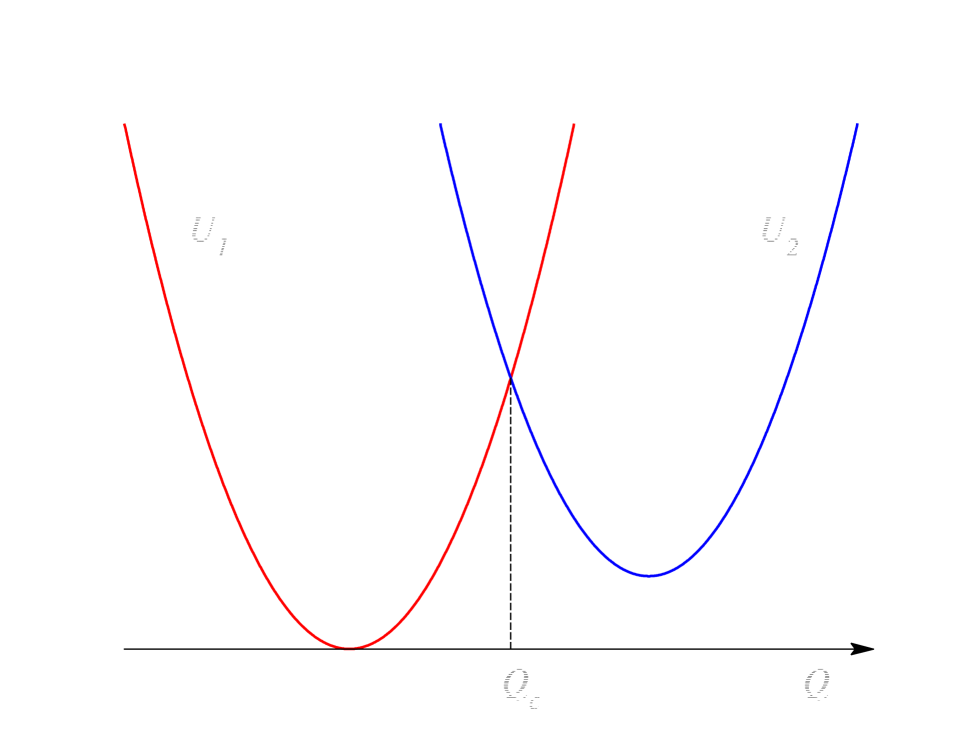
Figure 1: The schematic picture of the DCET model. The potential surfaces of the neutral (bright) and the charged (dark) electronic states are represented by the red and blue lines, respectively. Vertical dotted line corresponds to the crossing point.

Another interesting phenomenon that manifests in the emission of single quantum dots is the spectral diffusion showing characteristic time scales in the order of hundreds of seconds Empedocles et al. (1996); Empedocles and Bawendi (1999). It is not surprising that there are a number of models proposed to explain the blinking that relate the fluctuations in the emission intensity with slow variations in the exciton energy. The first model of that kind suggested by Shimizu et al. Shimizu et al. (2001) is based on the Efros/Rosen charging mechanism (CM) Efros and Rosen (1997). The CM attributes the ON and OFF periods to neutral and charged QDs, respectively. The light-induced electronic excitation in the charged QD is supposed to be quenched by a fast Auger recombination process. The model of Shimizu et al. Shimizu et al. (2001) assumes that the charging/discharging events happen when the energies of the neutral exciton and the charged state are in resonance. A more advanced version of this idea was used by Tang and Marcus in the DCET model Tang and Marcus (2005a, b). In 2014 Zhu and Marcus Zhu and Marcus (2014) presented an extension of the DCET model by introducing an additional biexciton charging channel.

Simultaneously with Tang and Marcus Tang and Marcus (2005a, b), another diffusion model based on the alternative fluctuating rate mechanism (FRM) of blinking was suggested by Frantsuzov and Marcus Frantsuzov and Marcus (2005). The FRM assumes that the non-radiative relaxation rate of the exciton is subject to long term fluctuations caused by the rearrangement of surface atoms. A basic life cycle of the QD within this mechanism begins with a photon absorption. A relaxation of the excited state can go in one of of two paths. The first path is relaxation via a photon emission. The second path is a hole trapping followed by a consequent non-radiative recombination with a remaining electron. The photoluminescence quantum yield (PLQY) of the QD emission in this case can be expressed as

$$Y(t)=\frac{k_{r}}{k_{r}+k_{t}(t)}\equiv k_{r}\tau_{av}$$ (2)

where $k_{r}$ is the radiative recombination rate, and $\tau_{av}$ is the averaged exciton lifetime. Thus the variations of the $k_{t}$ generate fluctuations of the emission intensity on a long time scale. The Frantsuzov and Marcus model Frantsuzov and Marcus (2005) connects the recombination rate with the fluctuating energy difference between 1S_e and 1P_e states.

In this article we are going to discuss the advantages and disadvantages of these models of single QD blinking based on spectral diffusion as well as their perspectives of further development.

II Diffusion-controlled electron transfer model

After introducing the Marcus reaction coordinate $Q$, DCET model equations describing the evolution of its probability distribution density in the neutral state $\varrho_{1}(Q,t)$ and in the charged state $\varrho_{2}(Q,t)$ can be written in the following form:

$$\frac{\partial}{\partial t}\varrho_{1}(Q,t)=D_{1}\frac{\partial}{\partial Q}\left(\frac{\partial}{\partial Q}+\frac{U_{1}^{\prime}(Q)}{kT}\right)\varrho_{1}(Q,t)$$

$$-2\pi\frac{V^{2}}{\hbar}\delta(U_{1}(Q)-U_{2}(Q))\left(\varrho_{1}(Q,t)-\varrho_{2}(Q,t)\right)$$ (3)

$$\frac{\partial}{\partial t}\varrho_{2}(Q,t)=D_{2}\frac{\partial}{\partial Q}\left(\frac{\partial}{\partial Q}+\frac{U_{2}^{\prime}(Q)}{kT}\right)\varrho_{2}(Q,t)$$

$$-2\pi\frac{V^{2}}{\hbar}\delta(U_{1}(Q)-U_{2}(Q))\left(\varrho_{2}(Q,t)-\varrho_{1}(Q,t)\right),$$ (4)

where $D_{1}$ and $D_{2}$ are diffusion coefficients in the neutral electronic state and charged state respectively, $V$ is the electronic coupling matrix element between the neutral and charged states, and $T$ is the effective temperature. The potential surfaces of the neutral $U_{1}(Q)$ and charged $U_{2}(Q)$ states are Marcus’ parabolas (see Fig. 1):

$$U_{1}(Q)=\frac{(Q+E_{r})^{2}}{4E_{r}}\qquad U_{2}(X)=\frac{(Q-E_{r})^{2}}{4E_{r}}+\Delta G$$ (5)

characterized by the reorganization energy $E_{r}$ and the free energy gap $\Delta G$. Transitions between the neutral and charged states are determined by the delta-functional sink in the crossing point $Q_{c}$ (local Golden rule), where $U_{1}(Q_{c})=U_{2}(Q_{c})$

$$Q_{c}=\Delta G$$

Equations (3-4) were initially introduced in 1980 independently by Zusman Zusman (1980) and Burshten and Yakobson Yakobson and Burshtein (1980) for describing solvent effects in electron transfer reactions. In the literature they are usually called Zusman equations (see for example the review article Barzykin et al. (2002) and references therein).The rigorous derivation of the Eqs. (3-4) from the basic quantum level (Spin-Boson Hamiltonian) was made in Ref. Frantsuzov (1999). The characteristic time scales of diffusion in the process of the electron transfer are of the order of picoseconds. That is to say that the equations (3-4) were originally designed to work for completely different time scales.

The statistics of the ON time blinking periods within the DCET model can be calculated using the function $\rho_{1}(Q,t)$ which is a solution of the equation (3) where the term describing the transfer from the charged state to the neutral one is omitted:

$$\frac{\partial}{\partial t}\rho_{1}(Q,t)=D_{1}\frac{\partial}{\partial Q}\left(\frac{\partial}{\partial Q}+\frac{U_{1}^{\prime}(Q)}{kT}\right)\rho_{1}(Q,t)$$

$$-2\pi\frac{V^{2}}{\hbar}\delta\left(U_{1}(Q)-U_{2}(Q)\right)\rho_{1}(Q,t)$$ (6)

with the initial condition describing the distribution function right after the transition from the charged state:

$$\rho_{1}(Q,0)=\delta(Q-Q_{c})$$

The probability of the ON state being longer than $t$ (survival probability) is defined by the integral of the function $\rho_{1}(Q,t)$

$$S_{\mbox{\tiny ON}}(t)=\int\limits_{-\infty}^{\infty}\rho_{1}(Q,t)\,dQ$$ (7)

The ON time distribution function is expressed as a derivative

$$p_{\mbox{\tiny ON}}(t)=-\frac{d}{dt}S_{\mbox{\tiny ON}}(t)$$ (8)

The analytical expression for the Laplace image of the ON time distribution function

$$\tilde{p}_{\mbox{\tiny ON}}(s)=\int\limits_{0}^{\infty}p_{\mbox{\tiny ON}}(t)e^{-st}\,dt$$

was found by Tang and Marcus Tang and Marcus (2005a, b) (derivation details are given in Appendix A):

$$\tilde{p}_{\mbox{\tiny ON}}(s)=\frac{Wg_{1}(s)}{1+Wg_{1}(s)}$$ (9)

where

$$W=\frac{\sqrt{2\pi}V^{2}}{\hbar\sqrt{E_{r}kT}}$$ (10)

Function $g_{1}(s)$ can be expressed as an integral

$$g_{1}(s)=\int\limits_{0}^{\infty}\frac{\exp\left[-st-\frac{x_{c}^{2}}{2}\tanh\left({\frac{t}{2\tau_{1}}}\right)\right]}{\sqrt{2\pi\left(1-e^{-2t/\tau_{1}}\right)}}\,dt$$ (11)

where $\tau_{1}$ is the relaxation time in the the neutral state

$$\tau_{1}=\frac{2E_{r}kT}{D_{1}}$$ (12)

and $x_{c}$ is the dimensionless crossing point coordinate

$$x_{c}=\frac{E_{r}+\Delta G}{\sqrt{2E_{r}kT}}$$ (13)

At a short time limit $t\ll\tau_{1}$ Tang and Marcus Tang and Marcus (2005a, b) presented the following approximation for the ON time distribution (see Appendix B):

$$p_{\mbox{\tiny ON}}(t)=\frac{\exp(-\Gamma_{1}t)}{\sqrt{\pi t_{c}t}}\left[1-\sqrt{\frac{\pi t}{t_{c}}}\exp\left(\frac{t}{t_{c}}\right)\mbox{erfc}\left(\sqrt{\frac{t}{t_{c}}}\right)\right]$$ (14)

where

$$\Gamma_{1}=\frac{x_{c}^{2}}{4\tau_{1}}$$ (15)

and $t_{c}$ is the critical time

$$t_{c}=\frac{4}{W^{2}\tau_{1}}$$ (16)

When $t$ is much shorter than the critical time Eq.(14) can be approximated as

$$p_{\mbox{\tiny ON}}(t)\approx\frac{1}{\sqrt{\pi t_{c}}}t^{-1/2},\quad t\ll t_{c}$$ (17)

when for longer times

$$p_{\mbox{\tiny ON}}(t)\approx\frac{1}{2}\sqrt{\frac{t_{c}}{\pi}}t^{-3/2}\exp(-\Gamma_{1}t),\quad t_{c}\ll t\ll\tau_{1}$$ (18)

The equation (18) reproduces the experimentally observed truncated power-law dependence Eq. (1). This dependence has to correspond to the power spectral density of the emission intensity $S(f)\sim f^{-3/2}$. The experimentally observed transition of the power spectral density dependence to $f^{-2}$ at large frequencies Pelton et al. (2007) was explained by the changing of the ON time distribution function behavior from (17) to (18) at times $t\sim t_{c}$.

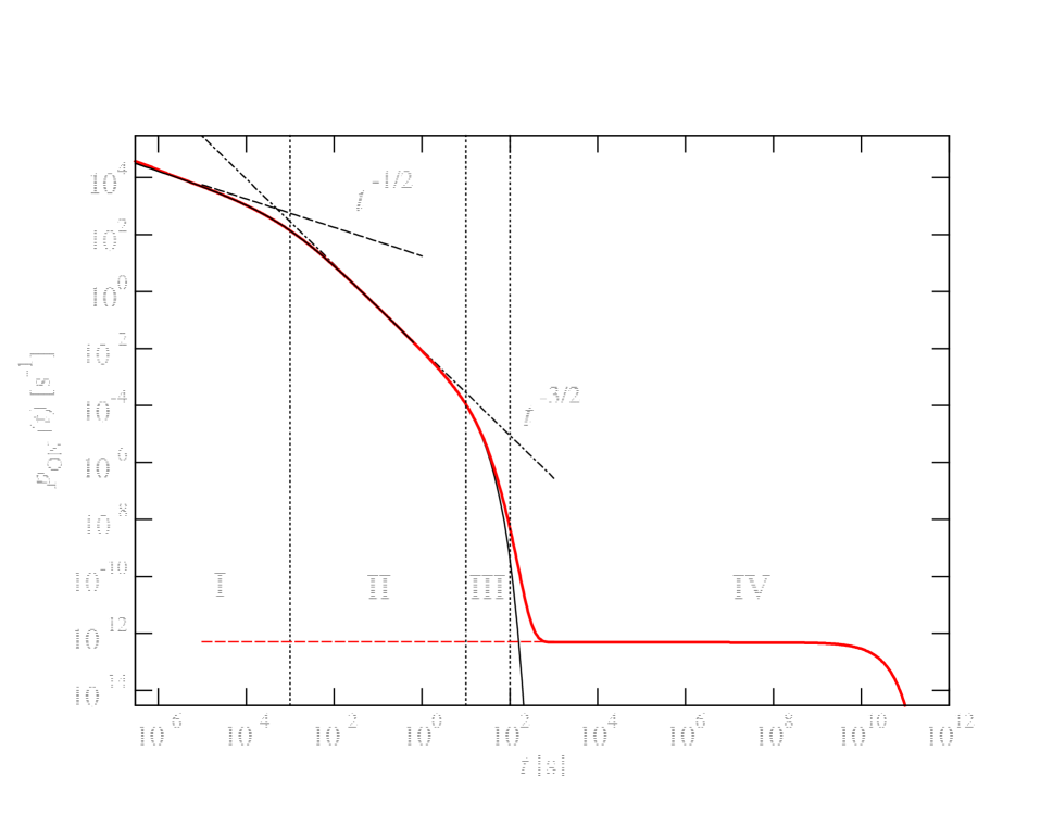
Figure 2: The ON time distribution function within the DCET model (thick red line), the first interval power law (black dashed line), the second interval power law (black dashed-dotted line), the Tang-Marcus approximation Eq.(14) (thin black line) and the long-time asymptotic Eq.(19) (red dashed line). Vertical dotted lines represent borders between characteristic intervals at $t_{c}$, $1/\Gamma_{1}$ and $\tau$. The parameters of the model are $\tau_{1}=100\,s$, $\Gamma_{1}=0.1\,s^{-1}$, $t_{c}=10^{-3}\,s$.

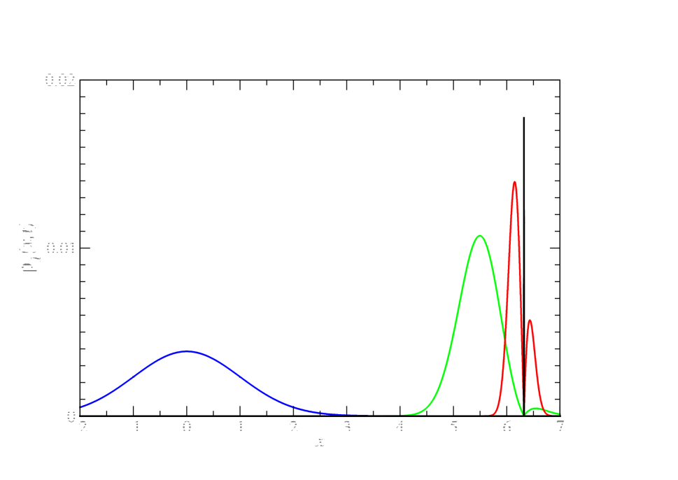
Figure 3: The coordinate probability distribution function $\rho_{1}(x,t=10^{-4}\,s)\times 10^{-4}$ (black line), $\rho_{1}(x,t=1\,s)\times 0.25$ (red line), $\rho_{1}(x,t=10.21\,s)$ (green line), $\rho_{1}(x,t=10^{5}\,s)$ (blue line). The parameters of the model are $\tau_{1}=100\,s$, $\Gamma_{1}=0.1\,s^{-1}$, $t_{c}=10^{-3}\,s$. $x$ is the dimensionless coordinate $x=(Q+E_{r})/\sqrt{2E_{r}kT}$

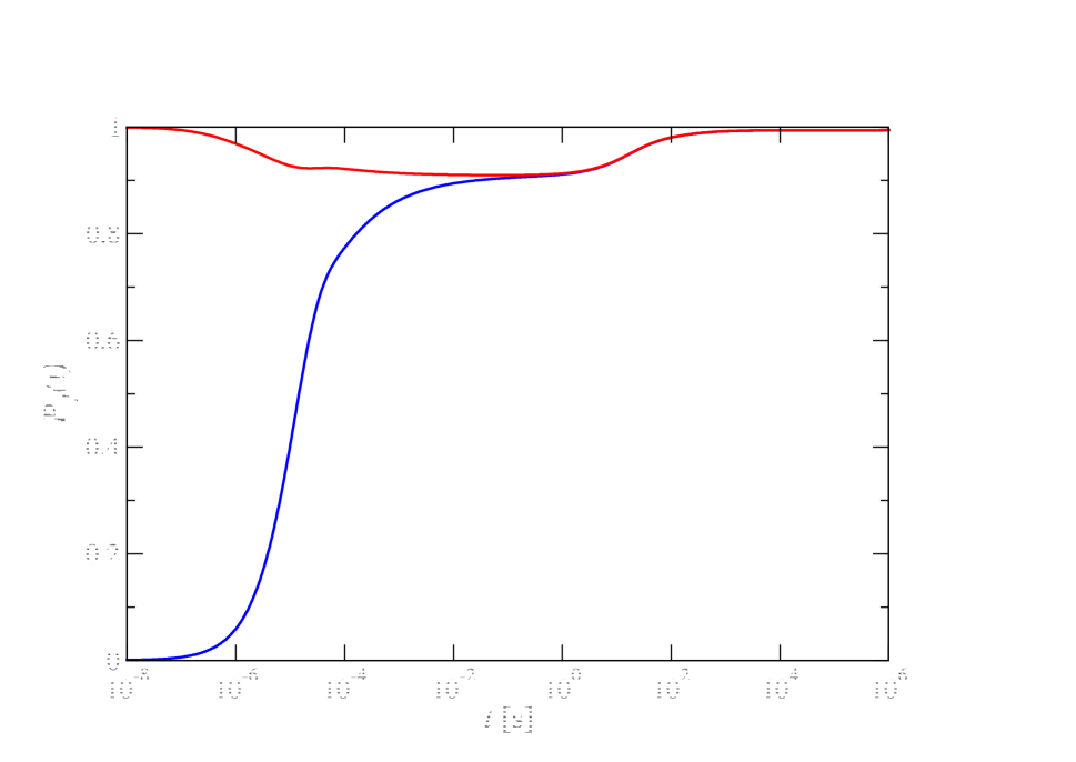
Figure 4: The time dependence of the probability of finding the QD in the neutral (bright) state for the initial condition (27) (red line) and the initial condition (28) (blue line). The parameters of the model are $\tau_{1}=100\,s$, $\Gamma_{1}=0.1\,s^{-1}$, $t_{c}=10^{-3}\,s$, $\tau_{2}=10^{4}\,s$, $\Gamma_{2}=10^{-3}\,s^{-1}$

The problem is that for longer times $t\gg\tau_{1}$ the approximate formula (14) is not applicable. It can be shown (see Appendix C) that at a very long time scale the ON time distribution shows slow exponential decay Tang and Marcus (2005b):

$$p_{\mbox{\tiny ON}}(t)\approx p_{1}\exp(-k_{1}t),\quad\tau_{1}\ll t$$ (19)

were $k_{1}$ is the decay rate

$$k_{1}=\frac{W}{\sqrt{2\pi}(1+WB)}\exp\left(-\frac{x_{c}^{2}}{2}\right)$$ (20)

$p_{1}$ is the amplitude

$$p_{1}=\frac{k_{1}}{1+WB}$$ (21)

and

$$B=\int\limits_{0}^{\infty}\left[\frac{\exp\left(-\frac{x_{c}^{2}}{2}\tanh\left({\frac{t}{2\tau_{1}}}\right)\right)}{\sqrt{2\pi\left(1-e^{-2t/\tau_{1}}\right)}}-\frac{\exp\left(-\frac{x_{c}^{2}}{2}\right)}{\sqrt{2\pi}}\right]\,dt$$

The last integral can be expressed in terms of a generalized hypergeometric function ${}_{2}F_{2}$ Burshtein et al. (1992):

$$B=\frac{\tau_{1}}{\sqrt{2\pi}}\exp\left(-\frac{x_{c}^{2}}{2}\right)\left[\ln 2+x_{c}^{2}\,{{}_{2}F_{2}}\left(\left.\begin{array}[]{cc}1&1\\ \frac{3}{2}&2\end{array}\right|\frac{x_{c}^{2}}{2}\right)\right]$$ (22)

The simpler analytical expressions of $B$ can be found in the limiting cases Burshtein et al. (1992):

$$B\approx\left\{\begin{array}[]{ll}\tau_{1}{\ln 2}/\sqrt{2\pi},&\quad|x_{c}|\ll 1\\ \tau_{1}/{|x_{c}|},&\quad|x_{c}|\gg 1\end{array}\right.$$ (23)

Equation (20) can be rewritten as

$$k_{1}=\frac{W}{\sqrt{2\pi}(1+WB)}\exp\left(-\frac{(E_{r}+\Delta G)^{2}}{4E_{r}kT}\right)$$ (24)

This formula is well-known in electron transfer theory Barzykin et al. (2002). It describes the quasi-stationary rate of the electron transfer in the absence of back transitions. The argument in the exponent reproduces the famous Marcus’ Free Energy Gap law. For low coupling values the rate Eq.(24) is proportional to $V^{2}$ (the Golden Rule result):

$$k_{1}=\frac{V^{2}}{\hbar\sqrt{E_{r}kT}}\exp\left(-\frac{(E_{r}+\Delta G)^{2}}{4E_{r}kT}\right)$$

At high coupling values the rate is limited by the diffusion transport to the crossing point and so becomes independent of $V$. For the activated process $(E_{r}+\Delta G)^{2}\gg 4E_{r}kT$ from Eqs.(24) and (23) we get:

$$k_{1}=\frac{|E_{r}+\Delta G|}{\tau_{1}\sqrt{4\pi E_{r}kT}}\exp\left(-\frac{(E_{r}+\Delta G)^{2}}{4E_{r}kT}\right)$$

The maximum rate is reached in the activationless case $(E_{r}+\Delta G)^{2}\ll 4E_{r}kT$

$$k_{1}=\frac{1}{\tau_{1}\ln 2}$$

As we can see the rate $k_{1}$ is always less than $1/\tau_{1}$.

The OFF time distribution shows a similar behaviour:

$$p_{\mbox{\tiny OFF}}(t)\approx\frac{1}{\sqrt{\pi t_{2}}}t^{-1/2},\quad t\ll t_{2}$$

$$p_{\mbox{\tiny OFF}}(t)\approx\frac{1}{2}\sqrt{\frac{t_{2}}{\pi}}t^{-3/2}\exp(-\Gamma_{2}t),\quad t_{2}\ll t\ll\tau$$

$$p_{\mbox{\tiny OFF}}(t)\approx p_{2}\exp(-k_{2}t),\quad\tau_{2}\ll t$$

where

$$\Gamma_{2}=\frac{x_{2}^{2}}{4\tau_{2}},\quad t_{2}=\frac{4}{W^{2}\tau_{2}}$$

$$k_{2}=\frac{W}{1+WB_{2}}\exp\left(-\frac{x_{2}^{2}}{2}\right),\quad p_{2}=\frac{k_{2}}{\sqrt{2\pi}(1+WB_{2})}$$

and

$$B_{2}=\frac{\tau_{2}}{\sqrt{2\pi}}\exp\left(-\frac{x_{2}^{2}}{2}\right)\left[\ln 2+x_{2}^{2}\,{{}_{2}F_{2}}\left(\left.\begin{array}[]{cc}1&1\\ \frac{3}{2}&2\end{array}\right|\frac{x_{2}^{2}}{2}\right)\right]$$ (25)

According to Eq.(14) and Eq. (19) there are four characteristic time intervals of the $p_{\mbox{\tiny ON}}(t)$ behavior:
Interval I: Power-law with $1/2$ exponent at $t\ll t_{c}$;
Interval II: Power-law with $3/2$ exponent at $t_{c}\ll t\ll 1/\Gamma_{1}$;
Interval III: Exponential decay at $1/\Gamma_{1}\ll t\ll\tau_{1}$;
Interval IV: Long time exponential decay $\tau_{1}\ll t$.
Note that Interval III can only exist if

$$\Gamma_{1}\tau_{1}\gg 1$$ (26)

We performed numerical simulations of Eq.(6) using the SSDP program Krissinel’ and Agmon (1996). The results of the simulations for the parameters $\tau_{1}=100\,s$, $\Gamma_{1}=0.1\,s^{-1}$, $t_{c}=10^{-3}\,s$ are presented in Fig. 2. The parameters are very close to the ones used in Ref.Tang and Marcus (2005a) for fitting the experimental data. The model parameters can be restored using Eqs.(15) and (10):

$$x_{c}=\sqrt{4\Gamma_{1}\tau_{1}}\approx 6.32,\quad W=\sqrt{\frac{4}{\tau_{1}t_{c}}}\approx 6.32\,s^{-1}$$

The condition $x_{c}\gg 1$ following from (26)is satisfied. Using Eq.(23) we get

$$BW=\frac{1}{\sqrt{\Gamma_{1}t_{c}}}=100$$

An expression for $k_{1}$ follows from Eq.(20)

$$k_{1}=\sqrt{\frac{2\Gamma_{1}}{\pi\tau_{1}}}\frac{\exp(-2\Gamma_{1}\tau_{1})}{1+\sqrt{\Gamma_{1}t_{c}}}\approx 5.15\times 10^{-11}\,s^{-1}$$

All four characteristic intervals of the ON time distribution dynamics are clearly seen on Fig. 2.

The value $p_{\mbox{\tiny ON}}(t)$ is very small at $t\gg\tau_{1}$ (interval IV), however the probability for the ON state to survive after $\tau_{1}$ time is quite significant.

$$S_{1}=S_{\mbox{\tiny ON}}(t\gg\tau_{1})\approx\int\limits_{0}^{\infty}p_{1}\exp(-k_{1}t)\,dt$$

From (21) we get

$$S_{1}\approx\frac{1}{1+BW}=\frac{\sqrt{\Gamma_{1}t_{c}}}{1+\sqrt{\Gamma_{1}t_{c}}}\approx 0.01$$

That is why the averaged ON time is extremely long:

$$\langle t_{\mbox{\tiny ON}}\rangle=\int\limits_{0}^{\infty}tp_{\mbox{\tiny ON}}(t)\,dt\approx\int\limits_{0}^{\infty}tp_{1}\exp(-k_{1}t)\,dt$$

and after integration:

$$\langle t_{\mbox{\tiny ON}}\rangle\approx\frac{k_{1}^{-1}}{1+BW}=\sqrt{\frac{\tau_{1}t_{c}}{2}}\exp(2\Gamma_{1}\tau_{1})\approx 1.08\times 10^{8}s$$

The coordinate probability distribution function $\rho_{1}(Q,t)$ within each interval is shown on Fig. 3. At a short time (Interval I) the distribution has one narrow maximum, its width increases with time $\Delta Q=\sqrt{2D_{1}t}$. The distribution function value at the crossing point $\rho_{1}(Q_{c},t)$ decays as $\sim t^{-1/2}$ and it follows the same power law form of the ON time distribution. At longer times (Interval II) the delta-functional sink burns a hole in the distribution function, and it shows two maxima. The distribution starts shifting towards the potential minimum within Interval III. That shifting generates an exponential decreasing of the $\rho_{1}(Q_{c},t)$ and as a result the exponential decay of the ON time distribution function. At times longer than $\tau_{1}$ (Interval IV) the function $\rho_{1}(Q,t)$ reaches the quasistationary distribution at the bottom of the parabolic potential

$$\rho_{1}(Q,t)\approx\frac{S_{1}}{\sqrt{4\pi E_{r}kT}}\exp\left(-\frac{(Q+E_{r})^{2}}{4E_{r}kT}\right)\exp(-k_{1}t)$$

As such, the transition to the OFF state can only occur at the $Q_{c}$ crossing point, which requires thermal activation. This explains why the decay of the ON time distribution is so gradual within Interval IV.

As seen from the analytical analysis and numerical simulations the DCET model predicts the appearance of extremely long ON time periods in a single QD emission trace. As seen on Fig. 2 such a period could last years, which is much longer than the duration of a typical experiment. The probability of such a long duration of a single ON time blinking event $S_{1}$ is found to be in order of 1%. Thus the QD can become permanently bright after about one hundred blinking cycles with a high probability.

All the predictions made about the ON time distribution can be applied for the OFF distribution as well. In most experiments the OFF time distribution truncation time of the single QD emission trace is too long to be detected. The only exceptions are the observations made on similar nanoobjects, namely nanorods S. Wang and et al. (2008) where the value $1/\Gamma_{2}\sim 2500\,s$ was found. Let us set $\Gamma_{2}=10^{-3}\,s^{-1}$ and $\tau_{2}=10^{4}\,s$. The corresponding rate for long time decay is $k_{2}\approx 5.15\times 10^{-13}\,s^{-1}$ The probability of an extremely long OFF time period is

$$S_{2}=\frac{\sqrt{\Gamma_{2}t_{2}}}{1+\sqrt{\Gamma_{2}t_{2}}}\approx 10^{-4}$$

This means that after about ten thousand blinking cycles the QD should become permanently bright or permanently dark. This prediction significantly differs from the behavior of single quantum dots observed in numerous experiments.

The fact that $S_{2}$ is much smaller than $S_{1}$ ($S_{2}/S_{1}\approx 10^{-2}$) suggests that the most of the QDs should became permanently bright. In order to verify that statement we used the SSDP program Krissinel’ and Agmon (1996) for numerical simulations of the Eqs.(3-4) with two types of initial conditions: at the beginning of the ON time period (delta-functional distribution in the neutral state)

$$\varrho_{1}(Q,0)=\delta(Q-Q_{c});\quad\varrho_{2}(Q,0)=0$$ (27)

and at the beginning of the OFF time period

$$\varrho_{1}(Q,0)=0;\quad\varrho_{2}(Q,0)=\delta(Q-Q_{c})$$ (28)

As shown in Fig. 4, the probability of finding the system in the ON state

$$P_{1}(t)=\int\limits_{-\infty}^{\infty}\varrho_{1}(Q,t)\,dQ$$

becomes very close to unity at times greater than 100 seconds for both cases.

III Extended DCET model

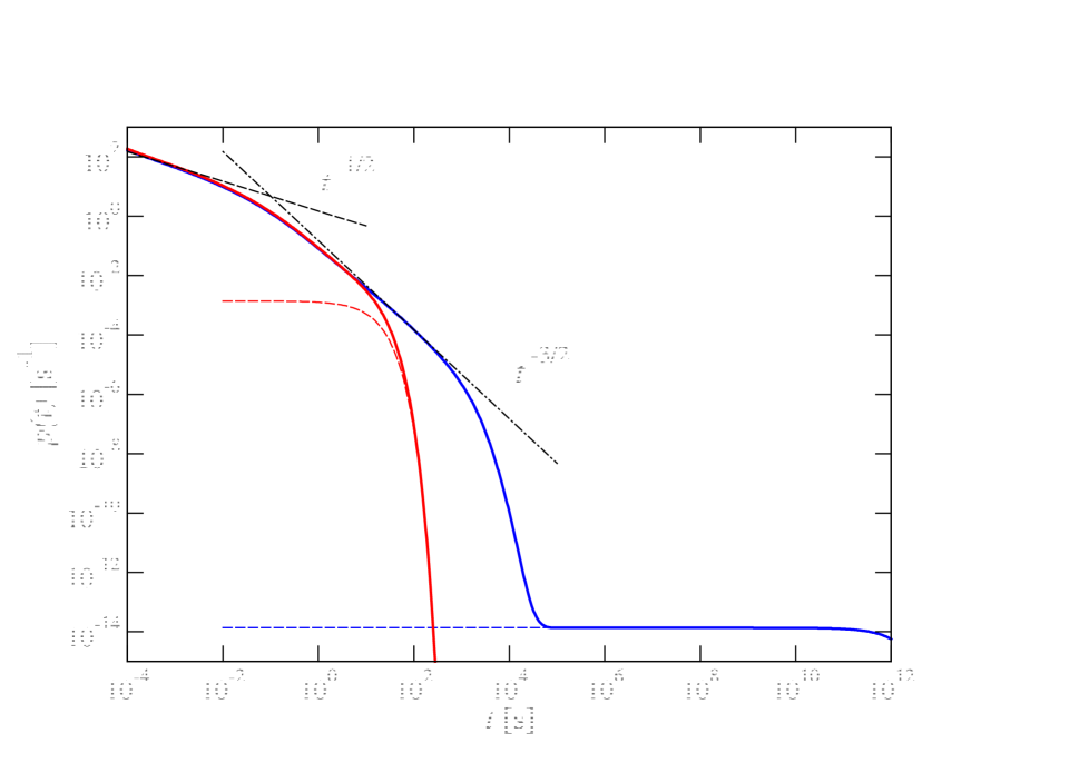
Figure 5: The ON time distribution function (thick red line) and the OFF time distribution function (thick blue line) within the Extended DCET model, the first interval power law (black dashed line), the second interval power law (black dashed-dotted line), the exponential decay of the ON time distribution Eq.(14) (dashed red line) and the OFF time distribution long-time asymptotic Eq.(19) (blue dashed line). The parameters of the model are $\tau_{1}=\tau_{2}=10^{4}\,s$, $\Gamma_{1}=\Gamma_{2}=10^{-3}\,s^{-1}$, $t_{c}=t_{2}=0.1\,s$, $K_{L}=10^{-1}\,s^{-1}$

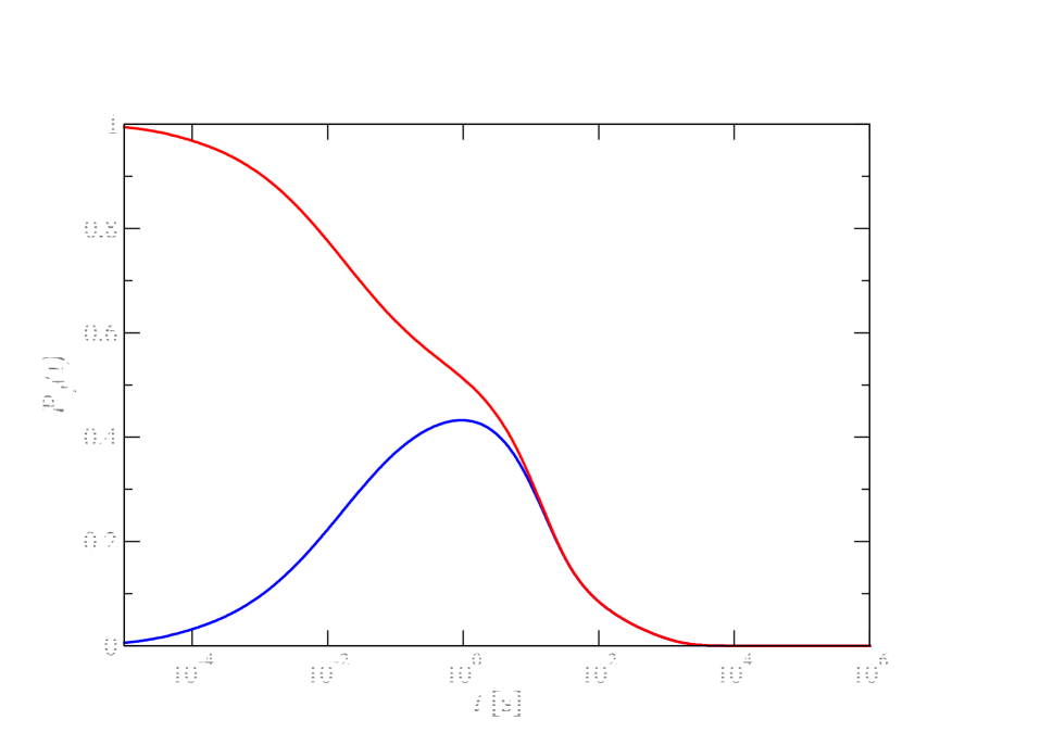
Figure 6: The time dependence of the probability of finding the QD in the neutral (bright) state for the initial condition (27) (red line) and the initial condition (28) (blue line) within the Extended DCET model. The parameters of the model are $\tau_{1}=\tau_{2}=10^{4}\,s$, $\Gamma_{1}=\Gamma_{2}=10^{-3}\,s^{-1}$, $t_{c}=t_{2}=0.1\,s$, $k_{L}=10^{-1}\,s^{-1}$

The extended DCET model of Zhu and Marcus Zhu and Marcus (2014) includes the equations describing the evolution of the probability density of the ground state $\varrho_{g}(Q,t)$, the excited state $\varrho_{e}(Q,t)$, the biexciton state $\varrho_{b}(Q,t)$, the charged (dark) state $\varrho_{d}(Q,t)$, and the excited dark state $\varrho_{d^{\ast}}(Q,t)$:

$$\frac{\partial}{\partial t}\varrho_{g}(Q,t)=k_{eg}\varrho_{e}(Q,t)-I_{ge}\varrho_{g}(Q,t)$$ (29)

$$\frac{\partial}{\partial t}\varrho_{e}(Q,t)=I_{ge}\varrho_{g}(Q,t)+L_{e}\varrho_{e}(Q,t)+k_{be}\varrho_{b}(Q,t)$$

$$-(k_{eg}+I_{eb})\varrho_{e}(Q,t)-k_{ed}\delta(Q-Q_{c})\varrho_{e}(Q,t)$$ (30)

$$\frac{\partial}{\partial t}\varrho_{b}(Q,t)=I_{eb}\varrho_{e}(Q,t)+L_{b}\varrho_{b}(Q,t)-(k_{be}+k_{bd^{\prime}})\varrho_{b}(Q,t)$$ (31)

$$\frac{\partial}{\partial t}\varrho_{d}(Q,t)=k_{d^{\ast}d}\varrho_{d^{\ast}}(Q,t)-I_{dd^{\ast}}\varrho_{d}(Q,t)$$ (32)

$$\frac{\partial}{\partial t}\varrho_{d^{\ast}}(Q,t)=L_{d^{\ast}}\varrho_{d^{\ast}}(Q,t)+I_{dd^{\ast}}\varrho_{d}(Q,t)$$

$$-k_{d^{\ast}d}\varrho_{d^{\ast}}(Q,t)-k_{d^{\ast}e}\delta(Q-Q_{c})\varrho_{d^{\ast}}(Q,t)$$ (33)

where $L_{e}$, $L_{b}$ and $L_{d^{\ast}}$ are diffusion operators

$$L_{e}=D_{e}\frac{\partial}{\partial Q}\left(\frac{\partial}{\partial Q}+\frac{U_{e}^{\prime}(Q)}{kT}\right)$$

$$L_{b}=D_{b}\frac{\partial}{\partial Q}\left(\frac{\partial}{\partial Q}+\frac{U_{b}^{\prime}(Q)}{kT}\right)$$

$$L_{d^{\ast}}=D_{d^{\ast}}\frac{\partial}{\partial Q}\left(\frac{\partial}{\partial Q}+\frac{U_{d^{\ast}}^{\prime}(Q)}{kT}\right)$$

$D_{e}$, $D_{b}$ $D_{d^{\ast}}$ are the diffusion coefficients, $U_{e}(Q)$, $U_{b}(Q)$ and $U_{d^{\ast}}(Q)$ are the potential surfaces of the excited state, the biexciton state and the dark excited state, respectively. $I_{ge}$, $I_{eb}$, $I_{dd^{\ast}}$, $k_{eg}$, $k_{be}$, $k_{bd^{\prime}}$, $k_{d^{\ast}d}$, $k_{d^{\ast}e}$, and $k_{ed}$ are the rate constants.

The equation for the probability density of the higher energy dark state has to be added to the equation system (29-33):

$$\frac{\partial}{\partial t}\varrho_{d^{\prime}}(Q,t)=k_{bd^{\prime}}\varrho_{b}(Q,t)-k_{d^{\prime}d}\varrho_{d^{\ast}}(Q,t)$$ (34)

As stated by Zhu and Marcus Zhu and Marcus (2014) quasiequilibrium is established between the ground, the excited state and the biexciton state. We can see from Eq. (34) that a quasistationary distribution of the the higher energy dark state is also determined by $\varrho_{e}(Q,t)$ and it can also can be considered a part of the quasiequilibrium. As such we can introduce the population of the integrated ON state

$$\varrho_{1}(Q,t)=\varrho_{g}(Q,t)+\varrho_{e}(Q,t)+\varrho_{b}(Q,t)+\varrho_{d^{\prime}}(Q,t)$$ (35)

Similarly, there is a quasiequilibrium between the dark and the excited dark states and the OFF state population can also be introduced

$$\varrho_{2}(Q,t)=\varrho_{d}(Q,t)+\varrho_{d^{\ast}}(Q,t)$$ (36)

The following kinetic equations for the functions $\varrho_{1}(Q,t)$ and $\varrho_{2}(Q,t)$ were obtained from Eqs. (29-34) (see Appendix D):

$$\frac{\partial}{\partial t}\varrho_{1}(Q,t)=L_{1}\varrho_{1}(Q,t)-k_{L}\varrho_{1}(Q,t)$$

$$-W_{1}\delta(Q-Q_{c})\varrho_{1}(Q,t)+W_{2}\delta(Q-Q_{c})\varrho_{2}(Q,t)$$ (37)

$$\frac{\partial}{\partial t}\varrho_{2}(Q,t)=L_{2}\varrho_{1}(Q,t)-W_{2}\delta(Q-Q_{c})\varrho_{2}(Q,t)$$

$$+W_{1}\delta(Q-Q_{c})\varrho_{1}(Q,t)+k_{LD}\varrho_{1}(Q,t)$$ (38)

where $L_{1}$ and $L_{2}$ are effective diffusion operators:

$$L_{1}=C_{1}\left(L_{e}+\frac{I_{eb}}{k_{be}}L_{b}\right);\quad L_{2}=C_{2}L_{d}$$

$W_{1}$, $W_{2}$ and $k_{L}$ are effective rates:

$$W_{1}=C_{1}k_{ed};\quad W_{2}=C_{2}k_{d^{\ast}e};\quad k_{L}=C_{1}k_{bd^{\prime}}\frac{I_{eb}}{k_{be}}$$

and $C_{1}$ and $C_{2}$ are the coefficients:

$$C_{1}=\left(1+\frac{k_{eg}}{I_{ge}}+\frac{I_{eb}}{k_{be}}+\frac{k_{bd^{\prime}}}{k_{d^{\prime}d}}\frac{I_{eb}}{k_{be}}\right)^{-1};\quad C_{2}=\left(1+\frac{k_{d^{\ast}d}}{I_{ge}}\right)^{-1}$$

We have to note that the equations derived by Zhu and Marcus ( Eqs.(11-12) in Ref.Zhu and Marcus (2014)) using the same procedure are different from Eqs. (37-38). The last term in Eq.(37) was omitted in Eq.(11) in Ref.Zhu and Marcus (2014) and the two last terms in Eq.(38) were omitted in Eq.(12) in Ref.Zhu and Marcus (2014). It can be seen that because of the absence of these terms, Eqs. (11-12) of Zhu and Marcus Zhu and Marcus (2014) do not preserve the total probability.

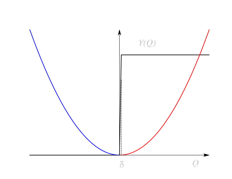
Figure 7: The schematic picture of the Frantsuzov and Marcus model. The potential surface is represented by a line colored red in the bright region ($Q>\delta$) and blue in the dark region ($Q<0$). The black line represents the PLQY dependence on the coordinate.

The ON time and OFF time distribution functions in the Extended DCET model (37-38) can be found by solving the following equations:

$$\frac{\partial}{\partial t}\rho_{1}(Q,t)=L_{1}\rho_{1}(Q,t)-W_{1}\delta(Q-Q_{c})\rho_{1}(Q,t)-k_{L}\rho_{1}(Q,t)$$ (39)

$$\frac{\partial}{\partial t}\rho_{2}(Q,t)=L_{2}\rho_{2}(Q,t)-W_{2}\delta(Q-Q_{c})\rho_{2}(Q,t)$$ (40)

Transitions from the dark state to the bright state occur only at the point $Q_{c}$, thus the initial distribution for the Eq. (39) is a delta-function:

$$\rho_{1}(Q,t)=\delta(Q-Q_{c})$$

in contrast transitions from a bright state to a dark state can occur not only at the crossing point and the initial condition for the Eq. (40) has the following form:

$$\rho_{2}(Q,t)=\int\limits_{0}^{\infty}(W_{1}\delta(Q-Q_{c})+k_{L})\rho_{1}(Q,t)\,dt$$

The Eq.(39) has an additional term $-k_{L}\rho_{1}(Q,t)$ in comparison to Eq.(6) which leads to an exponential cutoff of the survival probability (7) time dependence

$$S_{\mbox{\tiny ON}}(t)=S^{0}_{\mbox{\tiny ON}}(t)\exp(-k_{L}t)$$

where $S^{0}_{\mbox{\tiny ON}}(t)$ is the survival probability obtained from Eq. (39) at $k_{L}=0$. As a result the ON time distribution function in the Extended DCET model has an exponential cutoff.

$$p_{\mbox{\tiny ON}}(t)\sim\exp(-k_{L}t),\quad t\gg 1/k_{L}$$

The Eq.(40) is equivalent to Eq.(6). The difference in the initial distributions leads to the deviation of the OFF time distribution in the Extended DCET model in comparison with the original DCET model at times smaller than $\tau_{2}$. The long time exponential asymptotic behavior, however, is the same

$$p_{\mbox{\tiny OFF}}(t)\sim\exp(-k_{2}t),\quad t\gg\tau_{2}$$

These theoretical predictions are confirmed by numerical simulations (see Fig. 5) performed for the case of the symmetric system $Q_{c}=0$, $W_{1}=W_{2}$. The rest of the parameters are $\tau_{1}=\tau_{2}=10^{4}\,s$, $\Gamma_{1}=\Gamma_{2}=10^{-3}\,s^{-1}$, $t_{c}=t_{2}=0.1\,s$, $K_{L}=10^{-1}\,s^{-1}$. It can be concluded that the presence of a second ionization channel resolves the problem with very long ON times, but not with very long OFF times. As a result, most of the QDs in the Extended DCET model have to become permanently dark as confirmed by numerical simulations (see Fig. 6). That prediction also significantly differs from the experimentally observed behavior of single quantum dots.

IV Frantsuzov and Marcus model

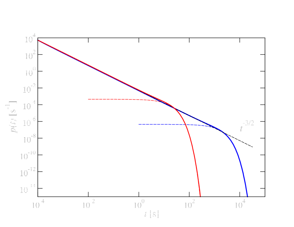
Figure 8: The normalized ON time (red thick line) and OFF time (blue thick line) distributions obtained by numerical simulations in the Frantsuzov and Marcus model, the $t^{-3/2}$ dependence (thin black line), $\exp(-t/T_{\mbox{\tiny ON}})$ (red dashed line), and $\exp(-t/T_{\mbox{\tiny OFF}})$ (blue dashed line). The parameters of the model are $T_{\mbox{\tiny ON}}=10$ s, $T_{\mbox{\tiny OFF}}=10^{3}$ s, $\delta=10^{-3}$, $\tau_{m}=10^{-4}$ s

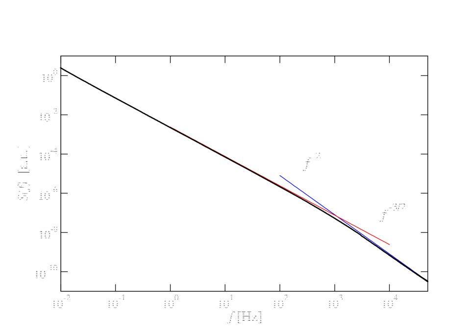
Figure 9: Power spectral density of the single QD fluorescence emission quantum yield (thick line) in the Frantsuzov and Marcus model, the $f^{-3/2}$ dependence (thin red line), and the $f^{-2}$ dependence (thin blue line). Parameters of the model are $T_{\mbox{\tiny ON}}=T_{\mbox{\tiny OFF}}=10^{3}$ s, $\delta=10^{-3}$.

The Frantsuzov and Marcus model Frantsuzov and Marcus (2005) is based on the fluctuating rate mechanism, thus it does not consider transitions between neutral and charged states. Fluctuations of the emission intensity in the model are caused by variations of the PLQY (2). The nonradiative recombination rate $k_{n}$ depends on the reaction coordinate $Q$ which is performing diffusive motion. Within the generalized formulation of the model the probability distribution function $\rho(Q,t)$ satisfies the equation

$$\frac{\partial}{\partial t}\varrho(Q,t)=\frac{\partial}{\partial Q}D(Q)\left(\frac{\partial}{\partial Q}+Q\right)\varrho(Q,t)$$ (41)

where $D(Q)$ is the coordinate dependent diffusion coefficient. To generate fast transitions from high to low emission intensity and back, the function $Y(Q)$ must grow dramatically from a minimal value to a maximum one on a tiny interval of $\delta$ close to the origin (see Fig. 7). Thus, the QD is bright when $Q>\delta$, dark when $Q<0$, and has some intermediate florescence intensity within the interval of $\delta\ll 1$. Taking into account that a molecular mechanism of the spectral diffusion is light induced Empedocles and Bawendi (1999); Fernee et al. (2010), the diffusion coefficient $D(Q)$ has to depend on the excitation intensity. It also means that the diffusion could be much faster for a bright QD than for a dark one Frantsuzov and Marcus (2005). As such, we can choose:

$$D(Q)=\left\{\begin{array}[]{ccl}1/{T_{\mbox{\tiny OFF}}},&&Q<0\\ 1/{T_{\mbox{\tiny ON}}},&\delta\leq&Q\end{array}\right.$$ (42)

It was shown by Frantsuzov and Marcus Frantsuzov and Marcus (2005) that the normalized ON time and OFF time distributions obtained by the threshold procedure have the following dependence (see Appendix E for details):

$$p(t)=\frac{\sqrt{\tau_{m}}}{2}t^{-3/2},\quad\tau_{m}\leq t\ll T_{0}$$ (43)

$$p(t)=\sqrt{\frac{2\tau_{m}}{T_{0}^{3}}}\exp(-t/T_{0}),\quad T_{0}\ll t$$ (44)

where $\tau_{m}$ is the minimum time interval of observation (bin time) and $T_{0}$ is equal to $T_{\mbox{\tiny ON}}$ and $T_{\mbox{\tiny OFF}}$ for the ON time and OFF time distribution, respectively. That prediction is confirmed by the numerical simulations made using the SSDP program Krissinel’ and Agmon (1996) (see Fig. 8).

The power spectral density $S(f)$ of the single QD emission at frequencies $f$ larger than $1/\tau_{m}$ could be obtained without binning procedure by measuring the autocorrelation function Pelton et al. (2004, 2007). In order to calculate $S(f)$ within the model one needs to specify the $Y(Q)$ function in the intermediate interval. Let’s choose the simplest linear dependence:

$$Y(Q)=\left\{\begin{array}[]{ccl}0,&&Q<0\\ Q/\delta,&0\leq&Q<\delta\\ 1,&\delta\leq&Q\end{array}\right.$$ (45)

The results of numerical calculations of the $S(f)$ in that case are presented in Fig. 9 (see Appendix F for the detailed calculation procedure). The Figure clearly shows the transition from the $f^{-3/2}$ dependence to $f^{-2}$ at large frequencies in accordance with the experiment of Pelton et al. Pelton et al. (2007).

V Discussion

As a result of the above analytical and numerical studies it was found that two models of single QD blinking based on spectral diffusion, namely the DCET model Tang and Marcus (2005a, b) and the Extended DCET model Zhu and Marcus (2014) predict that after an initial blinking period, most of the QDs should become permanently bright or permanently dark. That prediction significantly differs from the behavior of single quantum dots observed in numerous experiments. Another drawback of these models is the charging mechanism on which they are based. Despite the fact that most of the theoretical models proposed in the literature are based on that mechanism Kuno et al. (2001); Shimizu et al. (2001); Verberk et al. (2002); Margolin and Barkai (2004); Tang and Marcus (2005b); Osad ko (2013); Zhu and Marcus (2014), there is a number of sufficient experimental evidence indicating that the charging mechanism fails in explaining the QD blinking phenomenon. In several experiments, the emission intensity of a single QD was observed below the charged state (trion) emission intensity Zhao et al. (2010); Rosen et al. (2010); Tenne et al. (2013); Park et al. (2017). Another very important set of experiments showed that the existence of the distinct ON and OFF states is an illusion; there is a nearly continuous set of emission intensities Schlegel et al. (2002); Fisher et al. (2004); Zhang et al. (2006); Amecke and Cichos (2011); Schmidt et al. (2014). Furthermore, it was also shown Frantsuzov et al. (2009); Crouch et al. (2010); Amecke et al. (2014) that the parameters $m$ and $T$ of the ON and OFF time distributions strongly depend on the threshold value.

The Frantsuzov and Marcus model Frantsuzov and Marcus (2005), based on fluctuating rate mechanism, reproduces the key properties of the QD blinking phenomenon. Nonetheless there are a number of the experimental observations which are not explained by the model:
1. The exponent value $m$ of the ON and OFF time distribution functions is reported in the range from 1.2 to 2.0 Frantsuzov et al. (2008), and it strongly depends on the threshold value Frantsuzov et al. (2009); Crouch et al. (2010); Amecke et al. (2014). Meanwhile, in the model, $m$ is always equal to $3/2$ regardless of the threshold.
2. The exponent $r$ of the emission power spectral density is found to be in the range from 0.7 to 1.2 Pelton et al. (2004, 2007); Frantsuzov et al. (2013), when the model predicts the exponent value of 3/2.
3. The long-term correlations between subsequent ON and OFF times Stefani et al. (2005); Volkán-Kacsó et al. (2010). There are no such correlations in the model.

A possible reason for this discrepancy is that the description of the spectral diffusion in the model does not fully correspond to its real properties. It was shown that the squared frequency displacement of the single QD emission has an anomalous (sublinear) time dependence Plakhotnik et al. (2010). Plakhotnik et al. Plakhotnik et al. (2010) suggested an explanation of this behavior by introducing a number of stochastic two-level systems (TLS) having a wide spectrum of flipping rates. A similar idea was applied by Frantsuzov, Volkan-Kacso and Janko in the Multiple Recombination Center (MRC) model of single QD blinking Frantsuzov et al. (2009). The MRC model, based on the fluctuating rate mechanism, also reproduces the key properties the single QD blinking. But in addition it explains the power spectral density dependence close to $1/f$ Frantsuzov et al. (2013), the threshold dependence of the $m$ and $T$ values Frantsuzov et al. (2009), and the long-term correlations between subsequent blinking times Volkán-Kacsó et al. (2010). This suggests that the spectral diffusion and the fluctuations of the emission intensity of a single QD can be explained by an unified model, which could become a generalization of the Frantsuzov and Marcus model.

In conclusion, we analytically and numerically considered three models of the single QD emission fluctuations (blinking) based on spectral diffusion. Only one of them, the Frantsuzov and Marcus model Frantsuzov and Marcus (2005), reproduces the key properties of the phenomenon. The DCET model Tang and Marcus (2005a, b) and the Extended DCET model Zhu and Marcus (2014) predict that after an initial blinking period, most of the QDs should become permanently bright or permanently dark which is significantly different from the experimentally observed behavior.

Appendix A: An analytical solution for the blinking time distribution within the DCET model

Introducing a dimensionless coordinate $x$

$$x=\frac{Q+E_{r}}{\sqrt{2E_{r}kT}}$$

we can rewrite Eq. (6) as

$$\frac{\partial}{\partial t}\rho_{1}(x,t)=\frac{1}{\tau_{1}}\frac{\partial}{\partial x}\left(\frac{\partial}{\partial x}+x\right)\rho_{1}(x,t)$$

$$-W\delta(x-x_{c})\rho_{1}(x,t)$$ (46)

with the initial condition

$$\rho_{1}(x,0)=\delta(x-x_{c})$$

where the relaxation time $\tau_{1}$ is given by Eq.(12), $x_{c}$ is the dimensionless crossing point coordinate Eq.(13) and $W$ is given by Eq.(10) Applying Eq.(46), the ON time distribution function (8) can be expressed as

$$p_{\mbox{\tiny ON}}(t)=-\frac{d}{dt}\int_{-\infty}^{\infty}\rho_{1}(x,t)\,dx=W\rho_{1}(x_{c},t)$$ (47)

The Laplace image of the function $\rho_{1}(x,t)$

$$\tilde{\rho}_{1}(x,s)=\int_{0}^{\infty}\rho_{1}(x,t)e^{-st}\,dt$$

obeys the following equation

$$s\tilde{\rho}_{1}(x,s)-\delta(x-x_{c})=$$

$$\frac{1}{\tau_{1}}\frac{\partial}{\partial x}\left(\frac{\partial}{\partial x}+x\right)\tilde{\rho}_{1}(x,s)-W\delta(x-x_{c})\tilde{\rho}_{1}(x,s)$$ (48)

The Green’s function of the differential operator in Eq.(46) satisfies the equation

$$\frac{\partial}{\partial t}G(x,x^{\prime},t)=\frac{1}{\tau_{1}}\frac{\partial}{\partial x}\left(\frac{\partial}{\partial x}+x\right)G(x,x^{\prime},t)$$ (49)

with the initial condition

$$G(x,x^{\prime},0)=\delta(x-x^{\prime})$$

The Green’s function and the Laplace image satisfies the equation

$$s\tilde{G}(x,x^{\prime},s)-$$

$$\frac{1}{\tau_{1}}\frac{\partial}{\partial x}\left(\frac{\partial}{\partial x}+x\right)\tilde{G}(x,x^{\prime},s)=\delta(x-x^{\prime})$$ (50)

Using Eq.(50), Eq.(48) can be rewritten as

$$\tilde{\rho}_{1}(x,s)=\tilde{G}(x,x_{c},s)-W\tilde{G}(x,x_{c},s)\tilde{\rho}_{1}(x_{c},s)$$ (51)

From Eq.(51) we can find $\tilde{\rho}_{1}(x_{c},s)$

$$\tilde{\rho}_{1}(x_{c},s)=\frac{\tilde{G}(x_{c},x_{c},s)}{1+W\tilde{G}(x_{c},x_{c},s)}$$

The Laplace image of the ON time distribution Eq.(47) is given by

$$\tilde{p}_{\mbox{\tiny ON}}(s)=W\tilde{\rho}_{1}(x_{c},s)$$

Substituting Eq.(48) we get

$$\tilde{p}_{\mbox{\tiny ON}}(s)=\frac{W\tilde{G}(x_{c},x_{c},s)}{1+W\tilde{G}(x_{c},x_{c},s)}$$ (52)

Green’s function (49) is well-known:

$$G(x,x^{\prime},t)=\frac{1}{\sqrt{2\pi\left(1-e^{-2t/\tau_{1}}\right)}}\exp\left[-\frac{\left(x-x^{\prime}e^{-t/\tau_{1}}\right)^{2}}{2\left(1-e^{-2t/\tau_{1}}\right)}\right]$$ (53)

Introducing the function $g_{1}(s)$

$$g_{1}(s)=\tilde{G}(x_{c},x_{c},s)$$ (54)

we can express Eq.(52) in the form Eq.(9).

Appendix B: The ON time distribution at short times within the DCET model

At a short time limit $t\ll\tau_{1}$ one has to find the function $g_{1}(s)$ at $s\gg 1/\tau_{1}$. Expanding the exponent’s argument in the Eq. (11) we get

$$g_{1}(s)=\int_{0}^{\infty}\frac{\exp(-st-\Gamma_{1}t)}{\sqrt{4\pi t/\tau_{1}}}\,dt=\frac{1}{2}\sqrt{\frac{\tau_{1}}{s+\Gamma_{1}}}$$ (55)

where $\Gamma_{1}$ is given by Eq.(15) Substituting Eq.(55) into Eq.(9) gives

$$\tilde{p}_{\mbox{\tiny ON}}(s)=\frac{1}{1+\sqrt{(s+\Gamma_{1})t_{c}}}$$

and after the inverse Laplace transformation we get Eq. (14).

Appendix C: The ON time distribution at long times within the DCET model

The approximate formula (14) works for short times only. In order to see the behavior of the function $p_{\mbox{\tiny ON}}(t)$ at a long time limit $t\gg\tau_{1}$ one has to consider its Laplace image $\tilde{p}_{\mbox{\tiny ON}}(s)$ (11) at $s\to 0$. If we expand the function $g_{1}(s)$ (54) into a series on $s$:

$$g_{1}(s)\approx\frac{1}{s}A+B$$ (56)

where

$$A=\lim_{t\to\infty}G(x_{c},x_{c},t)$$

and

$$B=\int_{0}^{\infty}\{G(x_{c},x_{c},t)-A\}\,dt$$

The Green’s function (53) approaches the stationary distribution at long times

$$\lim_{t\to\infty}G(x,x^{\prime},t)=\frac{1}{\sqrt{2\pi}}\exp\left(-\frac{x^{2}}{2}\right)$$

Thus the constants $A$ and $B$ are

$$A=\frac{1}{\sqrt{2\pi}}\exp\left(-\frac{x_{c}^{2}}{2}\right)$$

$$B=\int_{0}^{\infty}\left[\frac{\exp\left(-\frac{1}{2}{x_{c}^{2}}\tanh\left({\frac{t}{2\tau_{1}}}\right)\right)}{\sqrt{2\pi\left(1-e^{-2t/\tau_{1}}\right)}}-A\right]\,dt$$

Substituting Eq.(56) into Eq. (9) we get the following dependence of $\tilde{p}_{\mbox{\tiny ON}}(s)$ at small $s$

$$\tilde{p}_{\mbox{\tiny ON}}(s)\approx\frac{WB}{1+WB}+\frac{p_{l}}{s+k}$$

which corresponds to the exponential behavior Eq. (19)of the ON time distribution function at long times.

Appendix D: The derivation of the evolution equations within the Extended DCET model

If $k_{eg}$ is much larger than all other rates in Eq. (30) a quasiequlibrium value of exciton population is established

$$\varrho_{e}(Q,t)\approx\frac{I_{ge}}{k_{eg}}\varrho_{d}(Q,t)$$ (57)

Similarly if $k_{be}$ is much larger than all other rates in Eq.31:

$$\varrho_{b}(Q,t)\approx\frac{I_{eb}}{k_{be}}\varrho_{e}(Q,t)$$ (58)

If $k_{d^{\prime}d}\gg k_{bd^{\prime}}$

$$\varrho_{d^{\prime}}(Q,t)\approx\frac{k_{bd^{\prime}}}{k_{d^{\prime}d}}\varrho_{b}(Q,t)\approx\frac{k_{bd^{\prime}}}{k_{d^{\prime}d}}\frac{I_{eb}}{k_{be}}\varrho_{e}(Q,t)$$ (59)

Substituting Eqs. (57-59) with the definition Eq. (35) into Eqs. (29-31) we get Eq.(37).

If $k_{d^{\ast}d}$ is much larger than all other rates in Eq. (33) a quasiequlibrium value of the dark exciton population is established

$$\varrho_{d^{\ast}}(Q,t)=\frac{I_{ge}}{k_{d^{\ast}d}}\varrho_{d}(Q,t)$$ (60)

Substituting Eq.(60) with the definition Eq.(36) into Eqs.(32-34) we obtain Eqs.(38).

Appendix E: The ON time and OFF time distributions within the Frantsuzov and Marcus model

The survival probability of the ON time within the Frantsuzov and Marcus model can be found as an integral

$$S_{\mbox{\tiny ON}}(t)=\int\limits_{0}^{\infty}\rho(Q,t)\,dQ$$ (61)

where $\rho(Q,t)$ is a solution of the following equation

$$\frac{\partial}{\partial t}\rho(Q,t)=\frac{1}{T_{\mbox{\tiny ON}}}\frac{\partial}{\partial Q}\left(\frac{\partial}{\partial Q}+Q\right)\rho(Q,t)$$ (62)

with an absorbing boundary condition at the border (the first passage time problem)

$$\left.\rho(Q,t)\right|_{Q=0}=0$$ (63)

The question of what to take as the initial distribution for the equation is not easily answered. There is the minimal time $\tau_{m}$ (bin time) of the ON time period which can be observed. In accordance with Eq.(62), if the ON time period is longer than $\tau_{m}$ then the coordinate $Q$ has reached values larger than $\sqrt{\tau_{m}/T_{\mbox{\tiny ON}}}$. We can take any distribution located at a distance less than $\sqrt{\tau_{m}/T_{\mbox{\tiny ON}}}$ from the origin as an initial one. For the sake of simplicity, we can take the initial distribution in the form of a delta function

$$\rho(Q,0)=\delta(Q-\Delta)$$ (64)

where

$$\delta\ll\Delta\ll\sqrt{\tau_{m}/T_{\mbox{\tiny ON}}}$$

The solution of Eqs.(62-64) is well known

$$\rho(Q,t)=G(Q,\Delta,t)-G(-Q,\Delta,t)$$ (65)

where $G(x,x^{\prime},t)$ is the Green’s function of the Eq.(62)

$$G(Q,Q^{\prime},t)=\frac{\exp\left\{-\frac{\left[Q-Q^{\prime}\exp(-t/T_{\mbox{\tiny ON}})\right]^{2}}{2\left(1-\exp(-2t/T_{\mbox{\tiny ON}})\right)}\right\}}{\sqrt{2\pi\left(1-\exp(-2t/{T_{\mbox{\tiny ON}}})\right)}}$$ (66)

Using Eq.(65) the survival probability (61) can be expressed as

$$S_{\mbox{\tiny ON}}(t)=\frac{\int\limits_{-b}^{b}\exp\left[-\frac{Q^{2}}{2\left(1-\exp(-2t/T_{\mbox{\tiny ON}})\right)}\right]\,dQ}{\sqrt{2\pi\left(1-\exp(-2t/T_{\mbox{\tiny ON}})\right)}}$$

where $b=\Delta\exp(-t/T_{\mbox{\tiny ON}})$. At times $t>\tau_{m}$ the expression can be rewritten as

$$S_{\mbox{\tiny ON}}(t)=\frac{2\Delta\exp(-t/T_{\mbox{\tiny ON}})}{\sqrt{2\pi\left(1-\exp(-2t/T_{\mbox{\tiny ON}})\right)}}$$

This expression has the following behavior in the limiting cases

$$S_{\mbox{\tiny ON}}(t)=\Delta\sqrt{\frac{T_{\mbox{\tiny ON}}}{\pi t}},\quad\Delta^{2}T_{\mbox{\tiny ON}}\ll t\ll T_{\mbox{\tiny ON}}$$ (67)

$$S_{\mbox{\tiny ON}}(t)=\Delta\sqrt{\frac{2}{\pi}}\exp(-t/T_{\mbox{\tiny ON}}),\quad T_{\mbox{\tiny ON}}\ll t$$ (68)

In the experiment one can see that only the ON times are longer than $\tau_{m}$, which means that the ON time distribution should be normalized as follows

$$\int\limits_{\tau_{m}}^{\infty}p_{\mbox{\tiny ON}}(t)\,dt=1$$

The normalization procedure is equivalent to scaling of the function $S_{\mbox{\tiny ON}}$ so that the following equality for the normalized survival probability is satisfied

$$\bar{S}_{\mbox{\tiny ON}}(\tau_{m})=1$$ (69)

Applying this normalization to Eqs. (67-68) we get

$$\bar{S}_{\mbox{\tiny ON}}(t)=\sqrt{\frac{\tau_{m}}{t}},\quad\tau_{m}\leq t\ll T_{\mbox{\tiny ON}}$$

$$\bar{S}_{\mbox{\tiny ON}}(t)=\sqrt{\frac{2}{T_{\mbox{\tiny ON}}}}\exp(-t/T_{\mbox{\tiny ON}}),\quad T_{\mbox{\tiny ON}}\ll t$$

From Eq.(8) we obtain the ON time distribution function

$$p_{\mbox{\tiny ON}}(t)=\frac{1}{2}\sqrt{\tau_{m}}t^{-3/2},\quad\tau_{m}\leq t\ll T_{\mbox{\tiny ON}}$$

$$p_{\mbox{\tiny ON}}(t)=\sqrt{\frac{2\tau_{m}}{T_{\mbox{\tiny ON}}^{3}}}\exp(-t/T_{\mbox{\tiny ON}}),\quad T_{\mbox{\tiny ON}}\ll t$$

Similarly the expression for the OFF time distribution function can be obtained

$$p_{\mbox{\tiny OFF}}(t)=\frac{1}{2}\sqrt{\tau_{m}}t^{-3/2},\quad\tau_{m}\leq t\ll T_{\mbox{\tiny OFF}}$$

$$p_{\mbox{\tiny ON}}(t)=\sqrt{\frac{2\tau_{m}}{T_{\mbox{\tiny OFF}}^{3}}}\exp(-t/T_{\mbox{\tiny OFF}}),\quad T_{\mbox{\tiny OFF}}\ll t$$

These expression are equivalent to the Eqs. (43-44).

Appendix F: The emission intensity autocorrelation function within the Frantsuzov and Marcus model

The autocorrelation function of the emission intensity within the FRM is

$$C(t)=\left\langle Y\left(Q(t)\right)Y\left(Q(0)\right)\right\rangle$$

where averaging is performed over the ensemble of realizations of the random process $Q(t)$. For the Frantsuzov and Marcus model the function $C(t)$ can be written as

$$C(t)=\int\limits_{-\infty}^{\infty}\int\limits_{-\infty}^{\infty}Y(Q)G(Q,Q^{\prime},t)Y(Q^{\prime})\varrho_{0}(Q^{\prime})\,dQdQ^{\prime}$$ (70)

where $G(Q,Q^{\prime},t)$ is the Green’s function of Eq. (41) and the stationary distribution $\varrho_{0}$ is

$$\varrho_{0}(Q)=\frac{1}{\sqrt{2\pi}}\exp(-\frac{1}{2}Q^{2})$$

Eq. (70) can be rewritten as

$$C(t)=\int\limits_{-\infty}^{\infty}Y(Q)\varrho(Q,t)\,dQ$$

where $\varrho(Q,t)$ is the solution of Eq. (41) with the initial condition

$$\varrho(Q,0)=Y(Q)\varrho_{0}(Q)$$

A numerical solution was obtained using the SSDP program Krissinel’ and Agmon (1996). The power spectral density was calculated using a cosine transform

$$S(f)=4\int\limits_{0}^{\infty}C(t)\cos(2\pi ft)\,dt$$

References

- Nirmal et al. (1996) M. Nirmal, B. O. Dabousi, B. M. G., J. J. Maklin, J. K. Trautman, T. D. Harris, and L. E. Brus, Nature 383, 802 (1996).
- Frantsuzov et al. (2008) P. A. Frantsuzov, M. Kuno, B. Jankó, and R. A. Marcus, Nat. Phys. 4, 519 (2008).
- Stefani et al. (2009) F. D. Stefani, J. P. Hoogenboom, and E. Barkai, Phys. Today , 34 (2009).
- Cichos et al. (2007) F. Cichos, C. von Borczyskowski, and M. Orrit, Curr. Opin. Colloid. Interface Sci. 12, 272 (2007).
- Gómez et al. (2006) D. Gómez, M. Califano, and P. Mulvaney, Phys. Chem. Chem. Phys. 8, 4989 (2006).
- Krauss and Peterson (2010) T. D. Krauss and J. J. Peterson, J. Chem. Phys. Lett. 1, 1377 (2010).
- Riley et al. (2012) E. A. Riley, C. M. Hess, and P. J. Reid, Int. J. Mol. Sci. 13, 12487 (2012).
- Schwartz and Oron (2012) O. Schwartz and D. Oron, Isr. J. Chem. 52, 992 (2012).
- Cordones and Leone (2013) J. A. Cordones and S. R. Leone, Chem. Soc. Rev. 42, 3209 (2013).
- Pelton et al. (2007) M. Pelton, G. Smith, N. F. Sherer, and R. A. Marcus, Proc. Natl. Acad. Sci. 104, 14249 (2007).
- Empedocles et al. (1996) S. A. Empedocles, D. J. Norris, and M. G. Bawendi, Phys. Rev. Lett. 77, 3873 (1996).
- Empedocles and Bawendi (1999) S. A. Empedocles and M. G. Bawendi, J. Phys. Chem. B 103, 1826 (1999).
- Shimizu et al. (2001) K. T. Shimizu, R. G. Neuhauser, C. A. Leatherdale, S. A. Empedocles, W. K. Woo, and M. G. Bawendi, Phys. Rev. B 63, 205316 (2001).
- Efros and Rosen (1997) A. L. Efros and M. Rosen, Phys. Rev. Lett. 78, 1110 (1997).
- Tang and Marcus (2005a) J. Tang and R. A. Marcus, J. Chem. Phys. 123, 054704 (2005a).
- Tang and Marcus (2005b) J. Tang and R. A. Marcus, Phys. Rev. Lett. 95, 107401 (2005b).
- Zhu and Marcus (2014) Z. Zhu and R. A. Marcus, Phys. Chem. Chem. Phys. 16, 25694 (2014).
- Frantsuzov and Marcus (2005) P. A. Frantsuzov and R. A. Marcus, Phys. Rev. B. 72, 155321 (2005).
- Zusman (1980) L. D. Zusman, Chem. Phys. 49, 295 (1980).
- Yakobson and Burshtein (1980) B. I. Yakobson and A. I. Burshtein, Chem. Phys. 49, 385 (1980).
- Barzykin et al. (2002) A. V. Barzykin, P. A. Frantsuzov, K. Seki, and M. Tachiya, Adv. Chem. Phys. Advances in Chemical Physics, 123, 511 (2002).
- Frantsuzov (1999) P. A. Frantsuzov, J. Chem. Phys. 111, 2075 (1999).
- Burshtein et al. (1992) A. I. Burshtein, P. A. Frantsuzov, and A. A. Zharikov, J. Chem. Phys. 96, 4261 (1992).
- Krissinel’ and Agmon (1996) E. B. Krissinel’ and N. Agmon, J. Comp. Chem. 17, 1085 (1996).
- S. Wang and et al. (2008) C. Q. S. Wang and, M. D. Fischbein, L. Willis, D. S. Novikov, C. H. Crouch, and M. Drndic, Nano Lett. 8, 4020 (2008).
- Fernee et al. (2010) M. J. Fernee, B. Littleton, T. Plakhotnik, H. Rubinsztein-Dunlop, D. E. Gomez, and P. Mulvaney, Phys. Rev. B 81, 155307 (2010).
- Pelton et al. (2004) M. Pelton, D. G. Grier, and P. Guyot-Sionnest, Appl. Phys. Lett. 85, 819 (2004).
- Kuno et al. (2001) M. Kuno, D. P. Fromm, H. F. Hammann, A. Gallagher, and D. J. Nesbitt, J. Chem. Phys. 115, 1028 (2001).
- Verberk et al. (2002) R. Verberk, A. van Oijen, and M. Orrit, Phys. Rev. B 66, 233202 (2002).
- Margolin and Barkai (2004) G. Margolin and E. Barkai, J. Chem. Phys. 12, 1566 (2004).
- Osad ko (2013) I. S. Osad ko, J. Phys. Chem. C 117, 11328 (2013).
- Zhao et al. (2010) J. Zhao, G. Nair, B. R. Fisher, and M. G. Bawendi, Phys. Rev. Lett. 104, 157403 (2010).
- Rosen et al. (2010) S. Rosen, O. Schwartz, and D. Oron, Phys. Rev. Lett. 104, 157404 (2010).
- Tenne et al. (2013) R. Tenne, A. Teitelboim, P. Rukenstein, M. Dyshel, T. Mokari, and D. Oron, ACS Nano 7, 5084 (2013).
- Park et al. (2017) Y.-S. Park, J. Lim, N. S. Makarov, and V. I. Klimov, Nano Lett. 17, 5607 (2017).
- Schlegel et al. (2002) G. Schlegel, J. Bohnenberger, I. Potapova, and A. Mews, Phys.Rev.Lett. 88, 137401 (2002).
- Fisher et al. (2004) B. R. Fisher, H.-J. Eisler, N. E. Stott, and M. G. Bawendi, J. Phys. Chem. B 108, 143 (2004).
- Zhang et al. (2006) K. Zhang, H. Chang, A. Fu, A. P. Alivisatos, and H. Yang, Nano Lett. 6, 843 (2006).
- Amecke and Cichos (2011) N. Amecke and F. Cichos, J. Lumin. 131, 375 (2011).
- Schmidt et al. (2014) R. Schmidt, C. Krasselt, C. Göhler, and C. von Borczyskowski, ACS Nano 8, 3506 (2014).
- Frantsuzov et al. (2009) P. A. Frantsuzov, S. Volkán-Kacsó, and B. Jankó, Phys. Rev. Lett. 103, 207402 (2009).
- Crouch et al. (2010) C. H. Crouch, O. Sauter, X. Wu, R. Purcell, C. Querner, M. Drndic, and M. Pelton, Nano Lett. 10, 1692 (2010).
- Amecke et al. (2014) N. Amecke, A. Heber, and F. Cichos, J. Chem. Phys. 140, 114306 (2014).
- Frantsuzov et al. (2013) P. A. Frantsuzov, S. Volkán-Kacsó, and B. Jankó, Nano Lett. 13, 402 (2013).
- Stefani et al. (2005) F. D. Stefani, X. Zhong, W. Knoll, M. Han, and M. Kreiter, New J. Phys. (2005).
- Volkán-Kacsó et al. (2010) S. Volkán-Kacsó, P. A. Frantsuzov, and B. Jankó, Nano Lett. 10, 2416 (2010).
- Plakhotnik et al. (2010) T. Plakhotnik, M. J. Fernee, B. Littleton, H. Rubinsztein-Dunlop, C. Potzner, and P. Mulvaney, Phys. Rev. Lett. 105, 167402 (2010).