Causes of Effects via a Bayesian Model Selection Procedure

Abstract

In causal inference, and specifically in the Causes of Effects problem, one is interested in how to use statistical evidence to understand causation in an individual case, and so how to assess the so-called probability of causation (PC). The answer relies on the potential responses, which can incorporate information about what would have happened to the outcome as we had observed a different value of the exposure. However, even given the best possible statistical evidence for the association between exposure and outcome, we can typically only provide bounds for the PC. Dawid et al. (2016) highlighted some fundamental conditions, namely, exogeneity, comparability, and sufficiency, required to obtain such bounds, based on experimental data. The aim of the present paper is to provide methods to find, in specific cases, the best subsample of the reference dataset to satisfy such requirements. To this end, we introduce a new variable, expressing the desire to be exposed or not, and we set the question up as a model selection problem. The best model will be selected using the marginal probability of the responses and a suitable prior proposal over the model space. An application in the educational field is presented.

Keywords: Causes of effects; Probability of causation; Fundamental conditions; Model selection; Reference population; Counterfactuals.

1 Introduction

The Causes of Effects (CoE) problem concerns the study of individual causation and explicitly refers to something happened to a well identified individual. This nuance of causation has received less attention than the study of the Effects of Causes (EoC), also called the general causation problem. Actually, in EoC, the aim is the prediction of an outcome after the realization of an alleged cause; in CoE, instead, we want to evaluate the Probability of Causation (PC), i.e. the probability the observed outcome would not have been realized if the alleged cause had not been made effective, despite the fact that the cause and the outcome were already observed. Since we always refer causation to a specific individual, for the sake of simplicity, we call her Ann.

A simplified CoE question is the following. “Ann had a headache and decided to take aspirin. Her headache went away. Was that caused by the aspirin?”

In CoE, to evaluate the probability of causation, formally defined in Section 2, the relevant questions are: How might one use experimental and/or observational data, gathered on a reference group to which Ann belongs? How would one find the characteristics shared with Ann by the group of individuals from which the data came? These problems, also called the “Group to individual” (G2i) issue in forensic science, have generated a large debate in legal circles (see Faigman et al. (2014) [10]).

The issue was extensively studied in the statistical literature from a technical and a philosophical point of view, reaching different and somewhat related results. Essential references are Dawid (2000; 2016), [6], [3] and Pearl (2009; 2015) [14], [15]. Even if their approaches follow different routes, they agree about the use of counterfactuals and potential outcomes originating from Neyman ([12]) and re-introduced in the modern literature by Rubin (1974) ([17]). The need for counterfactuals in CoE is well illustrated by the question: “What would be the probability of the response if no treatment had been provided to the individual in whom we are interested?” Since only the treatment can be assigned to the individual, the matter concerns a counterfactual, i.e. an event which assumes something different from what happened. Depending on the assumptions, different results emerge in the forms of a precise probability or bounds (see Section 3). Although not as specific as one would ideally like, such bounds can be of use. In particular, if the lower bound exceeds one-half, then, in civil cases, we can infer causality “on the balance of probabilities”. To evaluate the PC, we follow the approach of Dawid et al. (2016) [6], that identified and detailed three fundamental conditions used to estimate from the data upper and lower bounds for the probability of causation.

A related problem is the choice of the reference population. More specifically, how to find that group, from among those obtainable from partitioning the randomized experiment sample according to Ann’s characteristics, which best fulfills the fundamental conditions. How much information to take into account and how to select the best comparison group is a tricky issue, also because the choice of the reference class can affect significantly the conclusions of the inference.

The main aim of the present paper is to make the fundamental conditions operative by means of empirical testing of such underlying assumptions, in a way that comes up with the “best” comparison group. We set the question up as a Bayesian model selection problem, where each model specifies a particular choice (more or less detailed) for the characteristics to be included, shared by Ann and the other individuals participating in the study. The best model will be selected considering the marginal probabilities of the response and a satisfactory prior proposal in the model space. To this end, we introduce a new variable that expresses, for each individual in the study, the desire to receive the treatment or not. This variable allows introducing the fundamental conditions in the model selection procedure. Such a method can have various applications in sociology and education, as well as in medicine. We present an example in the field of education, where we investigate the relation between success in a test and whether or not a hint was received (taking into account the student’s preference for receiving or not receiving the hint). The structure of this paper is as follows. We first introduce the notation and we define formally the Probability of Causation (PC). After the review of some results in the CoE literature, see Section 3, we provide the assumptions we require, Section 4. Then, in Section 5, we detail how to find the reference sample suitable for evaluating CoE by a model selection procedure. After presenting the application in Section 6, we draw some final conclusions.

2 Notation

We first specify the notation we need to introduce our approach.
Given data obtained from an ideal large randomized study concerning $n$ individuals, drawn from a population to which Ann belongs, assume that the study records the outcome $R=\{0,1\}$ of a treatment $T=\{0,1\}$, which is supposed large enough that the sampling variability of the estimates is negligible. Let $H$ be a large set of variables $H=\{H_{1},\dots,H_{k}\}$, characteristic of both Ann and the individuals participating in the study, where we assume that each $H_{j}$, $j\in 1,\dots,k$ is discrete (or even dichotomous). We denote by $H^{A}$ the value that the set of variables $H$ has for Ann. Since Ann not only takes the aspirin but also expresses her desire to take it, we introduce a variable $E=\{0,1\}$ (for Ann $E=1$) expressing such a desire for each individual in the study. This variable, first proposed as an unobservable by Dawid (2011), is here considered observable. We also introduce the potential variables $R_{T}=\{0,1\}$, so that, if the triple $(T,R_{0},R_{1})$ were observed contemporaneously, it would be easy to solve the CoE problem by stating the probability of causation (PC), defined as

$$PC_{A} \stackrel{{\scriptstyle\triangle}}{{=}} \Pr(R_{0}=0|H^{A},T=1,R_{1}=1)$$ (1)

$$= \dfrac{\Pr(R_{0}=0,R_{1}=1|H^{A},T=1)}{\Pr(R_{1}=1|H^{A},T=1)}.$$

Unfortunately, $R_{0},R_{1}$ are not jointly estimable from the data, and consequently $PC_{A}$ cannot be evaluated without some further assumptions.

3 Some results from the literature

In epidemiology, $PC_{A}$ has often been expressed by the quantity referred to as the excess risk ratio (see for instance [16])

$$ERR = \dfrac{\Pr(R_{1}=1|H^{A})-\Pr(R_{0}=1|H^{A})}{\Pr(R_{1}=1|H^{A})}$$ (2)

and sometime evaluated in terms of the observational risk ratio,

$$ORR = 1-1/\dfrac{\Pr(R=1|H^{A},T=1)}{\Pr(R=1|H^{A},T=0)}.$$ (3)

The quantity (3), which plays an important role in the developments we consider, can be evaluated by using the data for the treated and untreated individuals coming from a randomized study or from observational data. The choice between these two sources of data depends on the assumptions. We review the following three contributions.

a)

Pearl, 2000 (Theorem 9.2.14) [13], showed that, under Exogeneity ($R_{0},R_{1}\hskip 4.2679pt\perp\perp\hskip 4.2679ptT|H^{A}$, i.e. the potential outcomes $(R_{0},R_{1})$ have the same joint distribution, among both treated and untreated study subjects sharing the same background information $H^{A}$ as Ann) and Monotonicity ($R_{0}=1\rightarrow R_{1}=1$, i.e. if Ann were to recover if untreated, she would certainly recover if treated), $PC_{A}$ is identified and equal to ORR, evaluated on observational data. This result is remarkable since it ends up with a precise probability. At the same time, these assumptions are not easily defensible: Exogeneity, also called Strong Ignorability, is reasonable for data coming from a randomized study but it is considered weak for observational data. Monotonicity, also called No Prevention, is apparently reasonable (the treatment cannot be obtain worse results than the placebo) but for some individuals, for example those allergic to a medical treatment, it may not hold. In any case, this latter assumption can not usually be verified.

b)

Tian and Pearl, 2000 [18] demonstrated that, relaxing Exogeneity but retaining Monotonicity, the evaluation of the probability of causation can be obtained in a more refined form as

$$PC_{A} = \dfrac{\Pr(R^{obs}=1|T=1,H^{A})-\Pr(R^{obs}=0|T=1,H^{A})}{\Pr(R^{obs}=1|T=1,H^{A})}+$$ (4)

$$+ \dfrac{\Pr(R^{obs}1|T=0,H^{A})-\Pr(R^{exp}=1|T=0,H^{A})}{\Pr(R^{obs}=1,T=1|H^{A})}$$

where $obs$ and $exp$ specify the source of the data (observational or experimental). This result points out that CoE has both an experimental and an observational nature. Data from a randomized experiment amount for no confounding, i.e. the desirable Exogeneity property can be assumed quite safely. At the same time, Ann made a choice to receive the treatment, i.e. she was not forced to receive it. Hence, a difference between $\Pr(R^{obs}=1|T=0,H^{A})$ and $\Pr(R^{exp}=1|T=0,H^{A})$ is plausible and must be taken into account. For instance, if Ann’s disease is at an advanced stage, she has little will to be treated because she perceives that her survival is almost independent of the treatment. Since expression (4) points out the double nature of CoE, its computation requires having data from two different surveys, and this can be problematic.

c)

Dawid et al. (2016) consider the possibility of evaluating CoE by using only data coming from a randomized experiment. The authors proceed in two steps. First they derive bounds for the probability of causation based on the potential outcomes and the constraints implied in their joint distribution. Interestingly, the relevant $PC_{A}$ lower bound is equal to ERR (see (2)).

$$PC_{A}>\max\{0,1-1/RR_{A}\}$$

where $RR_{A}$, the risk ratio, is

$$RR_{A}=\frac{\Pr(R_{1}=1|H^{A},T=1)}{\Pr(R_{0}=1|H^{A},T=1)}.$$ (5)

Specifically, a large lower bound is the minimum probability of observing the response opposite to that actually observed if the treatment were not provided, so demonstrating that a different story would have been possible if the treatment had not been applied.

The question is:

“Even accepting working with bounds, what cautions must be taken to estimate

$$\Pr(R_{1}=1|H^{A},T=1)$$ (6)

and

$$\Pr(R_{0}=1|H^{A},T=1)$$ (7)

from experimental data?”

To answer the question, the authors detailed three conditions, called the fundamental conditions, to be assumed so as to estimate upper and lower bounds for $PC_{A}$ based on the marginal probabilities of the response.

The three conditions are the following:

1. Exogeneity: Already defined in Section 3.

2. Comparability: Ann’s potential response, $R^{A}_{1}$, is comparable with those of the treated subjects having the same background characteristics $H^{A}$ as Ann.

3. Sufficiency: Ann’s potential response $R^{A}_{0}$ and those of the untreated subjects, all having the same background characteristics $H^{A}$ as Ann, are comparable.

While Exogeneity follows directly from randomization, the other two conditions deserve careful reasoning, so the authors restrict their approach to when we can make good arguments for the acceptability of these fundamental conditions.

4 Validating the fundamental conditions

Our proposal to evaluate the CoE consists in finding, among all the possible groups of individuals differing from the specification of $H$, that one that “best fits” the conditions of Comparability and Sufficiency. The problem of validating the assumptions is turned into the search for the most suitable group of experimental data supporting the fundamental conditions.

To take into account the experimental and observational nature of the CoE, we consider as observed the variable $E$, (see Section 2), the decision to receive the treatment. For Ann, this variable provides some indirect information about her state of health, in the light of which it would no longer be appropriate to consider her similar to individuals in a pure experimental study for which this information was not available. For this reason we extend our experimental data to include the desire of the individuals in the sample to be treated or not. We believe that it is possible to get this information from people who have accepted a randomized treatment and we also believe that this practice is much less troublesome than to have a double survey of the same population, as in Tian and Pearl (2000) ([18]) (see Section 3).

In this extended scenario, Comparability means that, conditional on my knowledge of the pre-treatment characteristics of Ann and the trial subjects, I regard Ann’s potential response as comparable with those of the sub-group identified by ($T=1,E=1$) having characteristics $H^{A}$. In the same framework, the Sufficiency condition refers to the counterfactual scenario in which Ann was not treated. In this case we do not have information about Ann’s response nor the information concerning her will to receive the treatment or not. Apparently, for $T=0$, we could imagine that Ann did not desire receive the treatment (so $E=0$) but it might also be possible that she did not have the drug available, but her wish was to receive it (so $E=1$). Our concern is to find the specification of $H$ that makes irrelevant the influence of $E$ on the responses in the untreated group. If we can obtain reasonable support for the condition $R_{0}\hskip 4.2679pt\perp\perp\hskip 4.2679ptE|H^{A}$, i.e. if

$$\Pr(R_{0}=1|H^{A},E=1)=\Pr(R_{0}=1|H^{A},E=0),$$ (8)

it would be possible to estimate (7) by $\Pr(R=1|H^{A},T=0)$ using the data of the untreated.

5 Model selection

To perform a selection from models characterized by different $H$, we need to compute the marginal probabilities of the observed responses of Ann and the individuals participating in the study. We assume a relevant effect of the treatment that can be modelled using partial exchangeability among treated and untreated individuals. Furthermore the Comparability condition establishes that we are not able to distinguish between Ann and the group of treated individuals who desire to receive the treatment (identified by $(T=1,E=1)$), sharing with Ann the same characteristics $H^{A}$, as it concerns the uncertainty of their responses to the treatment. Since Comparability focusses on the group with the same characteristics as Ann, we don’t need to detail the responses of the remaining individuals in the treated group, and we model them as exchangeable.

The Sufficiency condition requires that in the untreated group, individuals sharing Ann’s characteristics (despite the fact that for some of them $E=0$ and for others $E=1$) are considered exchangeable. Also here we are not interested in distinguishing between the remaining individuals in the untreated group (those not sharing Ann’s characteristics), so that the untreated group is modeled as partially exchangeable. Of course according to what characteristics are included in $H$, different individuals in the randomized sample will be compared with Ann. We have $2^{k}$ ways of selecting a set of characteristics from $H$. Let $J$ be one of these choices, identified as a subset of $\{1,\ldots,K\}$. Each choice of $J$ induces a partition of the sample (treated and untreated), which defines a model $M_{j}$.

Then, by assuming partial exchangeability and by using de Finetti’s representation theorem inside every specified exchangeable group, we can evaluate the probability of observing Ann and the group of responses, induced by different subsets of $H$.

In this way we turn the issue of finding the group most supporting the fundamental conditions into a model selection problem, solved, as usual, by computing the marginal probability of the data conditionally on different instantiations of $H$.

Restricted to the treated group, we denote by $A_{1,1}$ the set of individuals who desire to take the treatment and share the same characteristics as Ann, with $\bar{A}_{1,1}$ its complement, and with $\mathbf{r}_{A_{1,1}}$, $\mathbf{r}_{\bar{A}_{1,1}}$ the corresponding vector of responses, while $r_{A}$ denotes Ann’s response. In the untreated group, let $A_{0,e}$ be the sets of individuals considered, $e=\{0,1\}$, $A_{0}=A_{0,0}\cup A_{0,1}$ and $\bar{A}_{0}$ its complement. We extend these notations in the obvious way to the vectors of responses and to the mixing parameters. We have:

$$\Pr(r_{A},\mathbf{r}_{A_{1,1}},\mathbf{r}_{\bar{A}_{1,1}},\mathbf{r}_{A_{0,1}},\mathbf{r}_{A_{0,0}},\mathbf{r}_{\bar{A}_{0}})|M_{J})=$$

$$\int_{\Theta}\Pr(r_{A},\mathbf{r}_{A_{1,1}},\mathbf{r}_{\bar{A}_{1,1}},\mathbf{r}_{A_{0,1}},\mathbf{r}_{A_{0,0}},\mathbf{r}_{\bar{A}_{0}}\mid\theta_{A_{1,1}},\theta_{\bar{A}_{1,1}},\theta_{A_{0}},\theta_{\bar{A}_{0}},M_{j})\cdot$$

$$\cdot\pi(\theta_{A_{1,1}},\theta_{\bar{A}_{1,1}},\theta_{A_{0}},\theta_{\bar{A}_{0}})d\theta_{A_{1,1}}d\theta_{\bar{A}_{1,1}}d\theta_{A_{0}}d\theta_{\bar{A}_{0}}=$$

$$=\int_{\Theta}\Pr(r_{A},\mathbf{r}_{A_{1,1}},\mathbf{r}_{\bar{A}_{1,1}},\mathbf{r}_{A_{0,1}},\mathbf{r}_{A_{0,0}},\mathbf{r}_{\bar{A}_{0}}\mid\theta_{A_{1,1}},\theta_{\bar{A}_{1,1}},\theta_{A_{0}},\theta_{\bar{A}_{0}},M_{j})\cdot$$

$$\cdot\pi(\theta_{A_{1,1}})\pi(\theta_{\bar{A}_{1,1}})\pi(\theta_{A_{0}})\pi(\theta_{\bar{A}_{0}})d\theta_{A_{1,1}}d\theta_{\bar{A}_{1,1}}d\theta_{A_{0}}d\theta_{\bar{A}_{0}}=$$

$$\int_{\Theta_{A_{1,1}}}\Pr(r_{A},\mathbf{r}_{A_{1,1}}\mid\theta_{A_{1,1}},M_{J})\pi(\theta_{A_{1,1}})d\theta_{A_{1,1}}\cdot\int_{\Theta_{\bar{A}_{1,1}}}\Pr(\mathbf{r}_{\bar{A}_{1,1}}\mid\theta_{\bar{A}_{1,1}},M_{J})\pi(\theta_{\bar{A}_{1,1}})d\theta_{\bar{A}_{1,1}}\cdot$$

$$\cdot\int_{\Theta_{A_{0}}}\Pr(\mathbf{r}_{A_{0,1}},\mathbf{r}_{A_{0,0}}\mid\theta_{A_{0}},M_{J})\pi(\theta_{A_{0}})d\theta_{A_{0}}\cdot\int_{\Theta_{\bar{A}_{0}}}\Pr(\mathbf{r}_{\bar{A}_{0}}\mid\theta_{\bar{A}_{0}},M_{J})\pi(\theta_{\bar{A}_{0}})d\theta_{\bar{A}_{0}}$$

By the de Finetti’s Representation Theorem, the conditional probabilities of the responses are a mixture of a binomial model and a mixture distribution over the corresponding parameters $\theta$s that are assumed independent of each other. As a consequence the overall integral easily factorizes.

Now we provide expressions for the above integrals. All the details are in Appendix (8). We have:

$$\int_{\Theta_{A_{1,1}}}\Pr(r_{A},\mathbf{r}_{A_{1,1}}\mid\theta_{A_{1,1}},M_{J})\pi(\theta_{A_{1,1}})d\theta_{A_{1,1}}=\frac{x_{A_{1,1}}+1}{n_{A_{1,1}}+2}\cdot\frac{1}{n_{A_{1,1}}+1}$$ (9)

where $x_{A_{1,1}}$ is the number of successes in the group $A_{1,1}$ and $n_{A_{1,1}}=|A_{1,1}|$. The notation is extended in the obvious way in the other groups.

$$\int_{\Theta_{\bar{A}_{1,1}}}\Pr(\mathbf{r}_{\bar{A}_{1,1}}\mid\theta_{\bar{A}_{1,1}},M_{J})\pi(\theta_{\bar{A}_{1,1}})d\theta_{\bar{A}_{1,1}}=\frac{1}{n_{\bar{A}_{1,1}}+1}$$ (10)

$$\int_{\Theta_{A_{0}}}\Pr(\mathbf{r}_{A_{0,1}},\mathbf{r}_{A_{0,0}}\mid\theta_{A_{0}},M_{J})\pi(\theta_{A_{0}})d\theta_{A_{0}} =\dbinom{n_{A_{0,0}}}{x_{A_{0,0}}}\dbinom{n_{A_{0,1}}}{x_{A_{0,1}}}\dbinom{n_{A_{0,0}}+n_{A_{0,1}}}{x_{A_{0,0}}+x_{A_{0,1}}}^{-1}\cdot$$ (11)

$$\cdot\frac{1}{n_{A_{0,0}}+n_{A_{0,1}}+1}$$ (12)

$$\int_{\Theta_{\bar{A}_{0}}}\Pr(\mathbf{r}_{\bar{A}_{0}}\mid\theta_{\bar{A}_{0}},M_{J})\pi(\theta_{\bar{A}_{0}})d\theta_{\bar{A}_{0}}=\frac{1}{n_{\bar{A}_{0}}+1}$$ (13)

Readers might recognize the conditional Irving–Fisher exact test as part of (12). The result is not surprising since we are looking for the set of $H$ making $E$ irrelevant, and thus supporting the hypothesis of no-difference between the success ratio in the two groups. An illustration of the behavior of the hypergeometric for $n_{A_{0,0}}=n_{A_{0,1}}=10$ is given in Figure 1. High support to the model is achieved when the number of successes $x_{A_{0,0}}$ and $x_{A_{0,1}}$ is almost the same in the two groups.

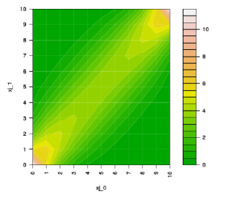
Figure 1: Hypergeometric behaviour for $n_{A_{0,0}}=n_{A_{0,1}}=10$ and different values for $x_{A_{0,0}}$ and $x_{A_{0,1}}$

5.1 Prior and posterior in the model space

The goal is to evaluate the posterior probability of $M_{J}$ given the responses observed for Ann and the sample. The overall marginal likelihood of $M_{j}$ is the product of (9), (10), (12) and (13)

$$\Pr(r_{A},\mathbf{r}_{A_{1,1}},\mathbf{r}_{\bar{A}_{1,1}},\mathbf{r}_{A_{0,1}},\mathbf{r}_{A_{0,0}},\mathbf{r}_{\bar{A}_{0}})|M_{J})=\frac{x_{A_{1,1}}+1}{n_{A_{1,1}}+2}\cdot\frac{1}{n_{A_{1,1}}+1}\cdot\frac{1}{n_{\bar{A}_{1,1}}+1}$$ (14)

$$\cdot \dbinom{n_{A_{0,0}}}{x_{A_{0,0}}}\dbinom{n_{A_{0,1}}}{x_{A_{0,1}}}\dbinom{n_{A_{0,0}}+n_{A_{0,1}}}{x_{A_{0,0}}+x_{A_{0,1}}}^{-1}\frac{1}{n_{A_{0,0}}+n_{A_{0,1}}+1}\cdot\frac{1}{n_{\bar{A}_{0}}+1}$$

Concerning the prior over the space of models, the simplest choice is to consider a uniform distribution

$$\Pr(M_{J})=\frac{1}{2^{k}}.$$ (15)

Another choice is the one proposed by Chen and Chen, (2008) [2]. They give the same prior probability (equal to $\frac{1}{k+1}$) for all models sharing the same number of characteristics $k$. In this way, for the generic model $M_{J}$, we have

$$\Pr(M_{J})=\frac{1}{k+1}\binom{k}{|M_{J}|}^{-1}\cdot I(|M_{J}|\leq k/2)$$ (16)

where the search spans all models including at most $k/2$ characteristics. This last choice favors model selection according to Occam’s razor principle: the fewer characteristics employed, the more probable is the model. This rationale is reasonably objective. Combining (15) or (16) with (14), we get the required posterior.

Computational issues

If the model size becomes huge, we may not be in a position to evaluate the normalizing constant of the posterior distribution, but we can establish an MCMC to make an inference about the variable $M_{J}$.

Essentially a Metropolis–Hastings would suffice, the acceptance ratio being given by (14), evaluated for two different elements of $M_{J}$, taking into account the probability of proposing a new model.

6 Application

We carried out an experiment at the University of Florence, School of Engineering, Fall 2017. We asked 161 students to solve a simple probabilistic question and we provided randomly a hint (the treatment $T$). Table (1) presents the students’ background information included in the analysis (the characteristics $H$). Before the test, we asked the students if they wished to be helped or not (the desire variable $E$).

Table 1: List of student characteristics included in the experiment

Variable Description 1 Engineer Course 0=Civil, 1= Facilities 2 Gender 0=male, 1=female 3 Age 0=$>21$, 1=$\geq 21$ 4 Place of birth 0= outside Florence, 1= Florence 5 Place of residence 0= outside Florence, 1= Florence 6 Year of Diploma 0=before 2016, 1=2016 7 Place of Diploma 0= outside Florence, 1= Florence 8 High school 0= Other, 1= Technical 9 Diploma vote 0= <80, 1= $\geq 80$ 10 $1^{st}$ registration at University 0= before 2016, 1=2016 11 Statistical background 0= no, 1=yes 12 Father’s level of education $0=\leq$ high school, 1=University 13 Mother’s level of education $0=\leq$ high school, 1=university 14 Working student 0=no, 1=yes

We wish to investigate whether there is a causal relation between the hint and the ability to solve the question, for those students who desired to receive a hint. We had 8 of these cases. The corresponding risk ratio (obtained considering the model best fitting the fundamental conditions) lies in the interval $[1.73,2.43]$ and in one case it exceeds $2$ ($RR=2.43$), which is a clue for there being a causal relation. In all the other cases, the causal relation is not strongly supported, since $RR$ is close but does not reach $2$ (see, in Figure (2)), the left side of each sub-picture). In the right side of each sub-picture in Figure(2) we illustrate how the model selection procedure proposes models respecting the fundamental conditions. For the model with the highest probability, the red dot indicates, in the $x-$axis, the success ratio for treated and, in the $y-$axis, the ratio between the success ratio for untreated with $E=1$ and with $E=0$, respectively. These are the main forces driving the marginal probability for the responses, as shown in (14). Ideally, comparability and sufficiency are mostly supported by the highest possible success ratio among the treated and by a ratio between untreated with E=0 and E=1 approximately equal 1. As is apparent, the selected model achieves a good compromise between these requirements. The set of variables selected in the 8 cases are shown in Table (2). Note that, overall, these models include only 5 characteristics, and all of them include the educational status of the family. In 4 out of the 8 cases, the same model, including family education, $1^{\text{first}}$ University registration (a proxy for understanding whether the student failed earlier in their educational career) and previous exposure to statistical training was selected.

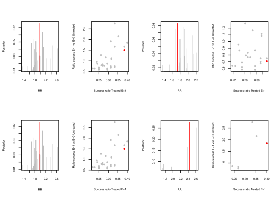
Figure 2: Educational causation. Risk Ratio and posterior probability for each explored model (left side). Success ratio for treated vs relative success ratio for untreated with $E=1$ and $E=0$ (right side). In the picture there is an example concerning four students who succeed.

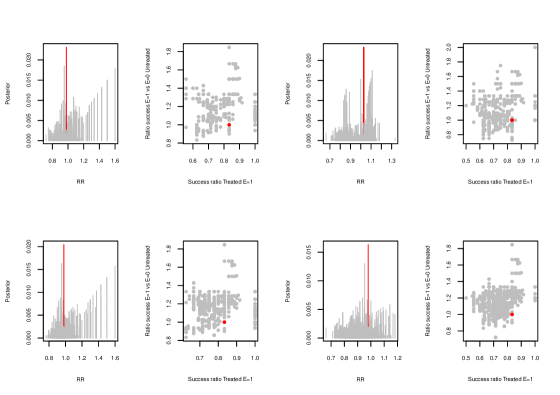
Figure 3: Forensic causation. Risk Ratio and posterior probability for each explored model (left side). Success ratio for treated vs relative success ratio for untreated with $E=1$ and $E=0$ (right side). In the picture there is an example concerning four students who DID NOT succeed.

Table 2: Educational causation. For the 8 students who desired the hint, got it, and succeed, there are reported the characteristics $H$ selected by the model that best supported the fundamental conditions and the Risk Ratio

Student $1^{st}$ University Statistical Education Work $RR$ registration background Father Mother 1 before $2016$ no university university $-$ $1.96$ 2 before $2016$ $-$ university university $-$ $1.73$ 3 $2016$ no university university $-$ $1.96$ 4 $-$ $-$ university university yes $2.43$ 5 before $2016$ $-$ university university yes $1.96$ 6 $2016$ no university university $-$ $1.96$ 7 $2016$ $-$ university university $-$ $1.96$ 8 $2016$ no university university $-$ $1.96$

As a result of our experiment we also have that among the students who asked for and received the hint, 24 did not succeed. We can suppose that some of them claimed that it was the hint which caused their failure. In this case, the $RR$ lies in the interval $[0.86,1.60]$, an example for four students is in Figure (3). It is not conclusive that there is a causal relation between the hint and the failure since all the models for all the considered students provided values of RR much smaller than 2. In a civil trial this would not suggest to a judge that compensation be awarded.

7 Conclusions

We introduced a typical Causes of Effects problem by means of an archetypical example considering Ann and the effect of an aspirin on her headache. We have proposed a possible solution to make operational the choice of variables to include, so as to validate the fundamental assumptions underlying the assessment of Ann’s probability of causation. We assume it is possible to take a randomized sample from Ann’s population where, as usual, $T$ is assigned following a randomized protocol and $E$ (this is a novelty) is a question asking the members of the sample about their preference to be treated or not.

In the evaluation of $RR_{A}$ (see 5), an extreme position would be to include all the subjects participating in the experiment so that simply belonging to the reference population would make the individuals in the sample similar to Ann. On the other hand, the choice could be to find the persons most similar to Ann, i.e. those matching all the available characteristics. Clearly neither of these positions is safe: the former ignores some characteristics of Ann which could be very influential on her reaction to the headache after taking aspirin. The latter greatly reduces the number of individuals to be employed in the estimation, so producing a very unstable inference. Our approach takes a sensible middle course and provide a sensible different causal inference for individuals experiencing the same treatment. Interestingly, this is exactly the aim of Precision Medicine (see Mesko (2017), [11]) which looks for different medical interventions for a group of individuals sharing some relevant (for the reaction between treatment and outcome) characteristics.

The next step will be to extend the method to observational studies, to make possible in a wider range of cases the evaluation of the $PC_{A}$ for Causes of Effects problems.

8 Appendix

Now we detail the computation of the integrals (9), (10), (12) and (13). We always assume a no informative prior for all $\pi(\cdot)=Beta(1,1)$. We start with (9).

$$\int_{\Theta_{A_{1,1}}}\Pr(r_{A},\mathbf{r}_{A_{1,1}}\mid\theta_{A_{1,1}},M_{J})\pi(\theta_{A_{1,1}})d\theta_{A_{1,1}}=$$

$$=\int_{\Theta_{A_{1,1}}}\Pr(r_{A}|\mathbf{r}_{A_{1,1}},\theta_{A_{1,1}},M_{J})\underbrace{\Pr(\mathbf{r}_{A_{1,1}}|\theta_{A_{1,1}},M_{J})\pi(\theta_{A_{1,1}}|M_{J})}_{\text{numerator of the }\theta_{A_{1,1}}\text{ updating}}d\theta_{A_{1,1}}$$

$$=\underbrace{\int_{\Theta_{A_{1,1}}}\Pr(r_{A}|\theta_{A_{1,1}},M_{J})\pi(\theta_{A_{1,1}}|\mathbf{r}_{A_{1,1}},M_{J})d\theta_{A_{1,1}}}_{\dfrac{x_{A_{1,1}}+1}{n_{A_{1,1}}+2}}\cdot$$

$$\cdot\underbrace{\int_{\Theta_{A_{1,1}}}\Pr(\mathbf{r}_{A_{1,1}}|\theta_{A_{1,1}},M_{J})\Pr(\theta_{A_{1,1}}|M_{J})d\theta_{A_{1,1}}}_{\dbinom{n_{A_{1,1}}}{x_{A_{1,1}}}\dfrac{\Gamma(1+1)}{\Gamma(1)\Gamma(1)}\dfrac{\Gamma(1+x_{A_{1,1}})\Gamma(n_{A_{1,1}}+1-x_{A_{1,1}})}{\Gamma(n_{A_{1,1}}+1+1)}}$$

$$=\frac{x_{A_{1,1}}+1}{n_{A_{1,1}}+2}\cdot\frac{1}{n_{A_{1,1}}+1}.$$

For (10) we have

$$\int_{\Theta_{\bar{A}_{1,1}}}\Pr(\mathbf{r}_{\bar{A}_{1,1}}\mid\theta_{\bar{A}_{1,1}},M_{J})\pi(\theta_{\bar{A}_{1,1}})d\theta_{\bar{A}_{1,1}}=$$

$$\underbrace{\int_{\Theta_{\bar{A}_{1,1}}}\Pr(\mathbf{r}_{\bar{A}_{1,1}}|\theta_{\bar{A}_{1,1}},M_{J})\Pr(\theta_{\bar{A}_{1,1}}|M_{J})d\theta_{\bar{A}_{1,1}}}_{\dbinom{n_{\bar{A}_{1,1}}}{x_{\bar{A}_{1,1}}}\dfrac{\Gamma(1+1)}{\Gamma(1)\Gamma(1)}\dfrac{\Gamma(1+x_{\bar{A}_{1,1}})\Gamma(n_{\bar{A}_{1,1}}+1-x_{\bar{A}_{1,1}})}{\Gamma(n_{\bar{A}_{1,1}}+1+1)}}$$

$$=\frac{1}{n_{\bar{A}_{1,1}}+1}$$

We now compute (12)

$$\int_{\Theta_{A_{0}}}\Pr(\mathbf{r}_{A_{0,1}},\mathbf{r}_{A_{0,0}}\mid\theta_{A_{0}},M_{J})\pi(\theta_{A_{0}},M_{J})d\theta_{A_{0}}=$$

$$=\int_{\Theta_{A_{0}}}\Pr(\mathbf{r}_{A_{0,0}},|\theta_{A_{0}},\mathbf{r}_{A_{0,1}},M_{J})\underbrace{\Pr(\mathbf{r}_{A_{0,1}}|\theta_{A_{0}},M_{J})\pi(\theta_{A_{0}}|M_{J})}_{\text{numerator of the }\theta_{A_{0}}\text{ updating}}d\theta_{A_{0}}$$

$$=\int_{\Theta_{A_{0}}}\Pr(\mathbf{r}_{A_{0,0}}|\theta_{A_{0}},M_{J})\pi(\theta_{A_{0}}|\mathbf{r}_{A_{0,1}},M_{J})d\theta_{A_{0}}\int_{\Theta_{A_{0}}}\Pr(\mathbf{r}_{A_{0,1}}|\theta_{A_{0}},M_{J})\pi(\theta_{A_{0}}|M_{J})d\theta_{A_{0}}$$

$$=\dbinom{n_{A_{0,0}}}{x_{A_{0,0}}}\dfrac{\Gamma(n_{A_{0,1}}+2)}{\Gamma(x_{A_{0,1}}+1)\Gamma(n_{A_{0,1}}-x_{A_{0,1}}+1)}\dfrac{\Gamma(x_{A_{0,1}}+1+x_{A_{0,0}})\Gamma(n_{A_{0,0}}+n_{A_{0,1}}-x_{A_{0,1}}+1-x_{A_{0,0}})}{\Gamma(n_{A_{0,0}}+n_{A_{0,1}}+2)}$$

$$\cdot\dbinom{n_{A_{0,1}}}{x_{A_{0,1}}}\dfrac{\Gamma(1+1)}{\Gamma(1)\Gamma(1)}\dfrac{\Gamma(1+x_{A_{0,1}})\Gamma(n_{A_{0,1}}+1-x_{A_{0,1}})}{\Gamma(n_{A_{0,1}}+1+1)}$$

$$=\dbinom{n_{A_{0,0}}}{x_{A_{0,0}}}\dbinom{n_{A_{0,1}}}{x_{A_{0,1}}}\dbinom{n_{A_{0,0}}+n_{A_{0,1}}}{x_{A_{0,0}}+x_{A_{0,1}}}^{-1}\frac{1}{n_{A_{0,0}}+n_{A_{0,1}}+1.}$$

Concerning the last term, (13), with a similar computation as for (10), it is straightforward to see that

$$\int_{\Theta_{\bar{A}_{0}}}\Pr(\mathbf{r}_{\bar{A}_{0}}\mid\theta_{\bar{A}_{0}},M_{J})\pi(\theta_{\bar{A}_{0}})d\theta_{\bar{A}_{0}}=\frac{1}{n_{\bar{A}_{0}}+1}.$$ (17)

Acknowledgement:The second author was supported by the project GESTA of the Fondazione di Sardegna and Regione Autonoma di Sardegna

References

- [1] Cheng, E.K., Law (2009) Statistics and the Reference Class Problem, Columbia Law Review, 109, 92–96.
- [2] Chen, J. and Chen, Z., (2008) Extended Bayesian Information Criteria for Model Selection with Large Model Spaces. Biometrika, 95, 3, 759–771.
- [3] Dawid, A. P. (2000), Causal Inference Without Counterfactuals. In Journal of the American Statistical Association, Vol. 95, No. 450 , pp. 407–424, 2000.
- [4] Dawid, A. P. (2011), The role of scientific and statistical evidence in assessing causality. In Perspectives on Causation, (ed. R. Goldberg), 133–147. Hart Publishing, Oxford .
- [5] Dawid, A. P., Faigman, D. L., and Fienberg, S. E. (2014), Fitting science into legal contexts: Assessing effects of causes or causes of effects? (with Discussion and authors’ rejoinder). Sociological Methods and Research, 43, 359–421 .
- [6] Dawid, A. P., Musio, M., and Fienberg, S. E. (2016), From Statistical Evidence to Evidence of Causality. Bayesian Analysis, 11, 725–752 .
- [7] Dawid, A. P., Murtas, R., and Musio, M. (2016), Bounding the probability of causation in mediation analysis. In Topics on Methodological and Applied Statistical Inference, (ed. T. D. Battista, E. Moreno, and W. Racugno) 75–84, Springer.
- [8] Dawid, A. P., Musio, M., and Murtas, R. (2017), The Probability of Causation, Law, Probability and Risk, 16, 4, 163–179.
- [9] de Finetti, B. (1970) Teoria delle Probabilità, Einaudi, Torino.
- [10] Faigman, D. L., Monahan, J., and Slobogin, C. (2014), Group to individual (G2i) inference in scientific expert testimony. University of Chicago Law Review, 81, 417–80.
- [11] Mesko, B. (2017), Expert Review of Precision Medicine and Drug Development. Journal Expert Review of Precision Medicine and Drug Development 2, 5, 239–241.
- [12] Neyman, J. (1923), On the application of probability theory to agricultural experiments. Essay on principles. Translated in Statistical Science, 5 4 465–472, 1990
- [13] Pearl, J. (2000), Causality: Models, Reasoning and Inference, 1st ed., Cambridge University Press.
- [14] Pearl, J. (2009), Causality: Models, Reasoning and Inference, 2nd ed., Cambridge University Press.
- [15] Pearl, J. (2015), Causes of Effects and Effects of Causes. Sociological Methods and Research, 44 (1), 149–164.
- [16] Rothman, K. J. (2012), Epidemiology: An Introduction 2nd ed., Oxford University Press.
- [17] Rubin, D. B.(1974), Estimating Causal Effects of Treatments in Randomized and Nonrandomized Studies. Journal of Educational Psychology, 66, 688–701.
- [18] Tian, J., and Pearl, J.(2010), Probabilities of Causation: Bounds and identification. Annals of Mathematics and Artificial Intelligence, 28, 287–313.