Longest increasing path within the critical strip

Abstract.

A Poisson point process of unit intensity is placed in the square $[0,n]^{2}$. An increasing path is a curve connecting $(0,0)$ with $(n,n)$ which is non-decreasing in each coordinate. Its length is the number of points of the Poisson process which it passes through. Baik, Deift and Johansson proved that the maximal length of an increasing path has expectation $2n-n^{1/3}(c_{1}+o(1))$, variance $n^{2/3}(c_{2}+o(1))$ and that it converges to the Tracy-Widom distribution after suitable scaling. Johansson further showed that all maximal paths have a displacement of $n^{\frac{2}{3}+o(1)}$ from the diagonal with probability tending to one as $n\to\infty$. Here we prove that the maximal length of an increasing path restricted to lie within a strip of width $n^{\gamma},\gamma<\frac{2}{3}$, around the diagonal has expectation $2n-n^{1-\gamma+o(1)}$, variance $n^{1-\frac{\gamma}{2}+o(1)}$ and that it converges to the Gaussian distribution after suitable scaling.

1. Introduction

The problem of determining the distribution of the length $\tilde{L}_{n}$ of the longest increasing subsequence in a random uniform permutation of $\{1,2,\cdots,n\}$ was first posed by Ulam and considered by Hammersley in his seminal paper [20]. It has since attracted a lot of attention in the mathematical community; see Romik’s book [33] for a lively history of this problem and the remarkable progress that has been made since it was first introduced. Using the subadditive ergodic theorem, Hammersley [20] was able to show the existence of a constant $c$ such that $\tilde{L}_{n}/\sqrt{n}\to c$ in probability as $n\to\infty$. A few years later, Logan and Shepp [28], and Vershik and Kerov [39] were able to compute the exact value $c=2$ using an analysis of random Young tableaux. A different proof was provided by Aldous and Diaconis [1] by studying of the hydrodynamical limit of an interacting particle system implicit in the work of Hammersley, which is now called the Hammersley process in his honor.

The above results can be considered as a law of large numbers for $\tilde{L}_{n}$. The limiting distribution for $\tilde{L}_{n}$, under appropriate centering and scaling, was found to be the Tracy-Widom distribution in the landmark paper by Baik, Deift and Johansson [5]. The paper is a tour-de-force using the Robinson-Schensted-Knuth correspondence between permutations and Young tableaux, and elements of Riemann-Hilbert theory. It is convenient to work with the following equivalent formulation of the problem, as done already by Hammersley [20] and as we will do in the rest of the paper. Consider a Poisson point process of unit intensity in the square $[0,n]^{2}$. Let $P_{n}$ be the (random) number of points inside the square. An increasing path is a curve connecting $(0,0)$ with $(n,n)$ which is non-decreasing in each coordinate. Its length is the number of points of the Poisson process which it passes through. Denote by $L_{n}$ the length of the longest increasing path. The relation between $L_{n}$ and $\tilde{L}_{n}$ is given by the fact, which is straightforward to check directly, that conditioned on $P_{n}=k$, the distribution of $L_{n}$ equals the distribution of $\tilde{L}_{k}$. One can therefore obtain the limiting distribution of $\tilde{L}_{P_{n}}$ by studying the Poissonized problem, and obtain similar results for $\tilde{L}_{n}$ via a de-Poissonization argument. Among the key findings of [5] is that, as $n\to\infty$,

$$\operatorname{\mathds{E}}L_{n}=2n-n^{1/3}(c_{1}+o(1)),$$ (1)

$$\operatorname{Var}L_{n}=n^{2/3}(c_{2}+o(1)),$$ (2)

$$\frac{L_{n}-\operatorname{\mathds{E}}L_{n}}{\sqrt{\operatorname{Var}L_{n}}}\text{ converges in distribution to the Tracy-Widom distribution}$$ (3)

with $c_{1},c_{2}>0$ absolute constants.

In a subsequent development, Johansson [27] showed using a geometric argument that the transversal exponent of the longest increasing path is $\frac{2}{3}$. More precisely, as the longest increasing path in $[0,n]^{2}$ need not be unique, it is shown there that with probability tending to $1$ as $n\to\infty$ all the longest increasing paths have a displacement of order $n^{\frac{2}{3}+o(1)}$ around the diagonal. The result raises the question of studying the maximal length attainable for increasing paths restricted to lie closer to the diagonal. Addressing this question is the main purpose of this paper.

Let $0<\gamma<\frac{2}{3}$ and set $L_{n}^{(\gamma)}$ to be the maximal length of an increasing path restricted to lie in $[0,n]^{2}\cap\{(x,y)\colon|y-x|\leqslant n^{\gamma}\}$. As $\gamma$ decreases, the length $L_{n}^{(\gamma)}$ corresponds to a maximum over a smaller set. It is then clear that $L_{n}^{(\gamma)}$ decreases and one may further

Theorem 1.1.

Fix $0<\gamma<\frac{2}{3}$. We have the following asymptotic behavior as $n\to\infty$:

$$\begin{split}\operatorname{\mathds{E}}L_{n}^{(\gamma)}&=2n-n^{1-\gamma+o(1)},\\ \operatorname{Var}L_{n}^{(\gamma)}&=n^{1-\frac{\gamma}{2}+o(1)}\end{split}$$ (4)

and

$$\frac{L_{n}^{(\gamma)}-\operatorname{\mathds{E}}L_{n}^{(\gamma)}}{\sqrt{\operatorname{Var}{L_{n}^{(\gamma)}}}}\Rightarrow N(0,1).$$ (5)

The Theorem is further refined by the results in Section 1.1 below.

The Gaussian fluctuations of the length of the longest increasing path inside the strip $n^{\frac{2}{3}-\epsilon}$ are remarkably different from the Tracy-Widom fluctuations of the length of the longest path within the strip $n^{\frac{2}{3}+\epsilon}$. A tantalizing problem would be to study the transition when paths within the critical strip, having width of order $n^{\frac{2}{3}}$, are considered.

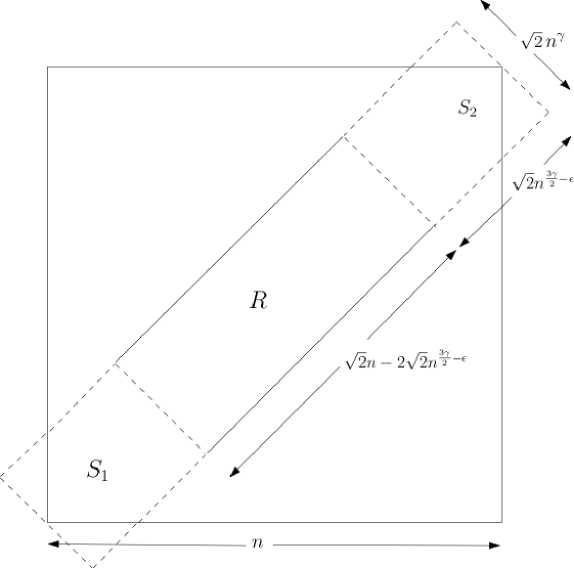
Figure 7. The regions $S_{1},R$ and $S_{2}$.

The heuristic for the proof is as follows. Partition the strip $[0,n]^{2}\cap\{(x,y)\colon|y-x|\leqslant n^{\gamma}\}$ into $n^{1-\frac{3\gamma}{2}+o(1)}$ diagonally-aligned rectangles (which we shall call blocks) of length $n^{\frac{3\gamma}{2}+o(1)}$ (the strip is partitioned apart from initial and final portions which are small enough to be ignored; see Figure 7). The length of the longest increasing path within each block obeys the scaling given by (1), (2) as the height of each block is larger than the $2/3$-power of its length, allowing for transversal fluctuations which are essentially unrestricted due to the result of [27]. If the length of the longest increasing path (LIP) in the entire strip was the sum of the lengths of the LIPs within each block, then we would have a sum of i.i.d. random variables and we could apply the Lindeberg-Feller theorem to get our result. However, this is not true – the restriction of a LIP (in the entire strip) to a block need not be maximal within this block. A key ingredient in our proof is Theorem 6.1, as a consequence of which we are able to show the existence of many blocks with regeneration points (these are the points $\mathbf{p}$ in (23)). A longest increasing path within the entire strip is obtained by concatenating the longest increasing paths between successive regeneration points. The regeneration points provide the necessary independence structure required for a Gaussian limit.

A model related to the above is directed last passage percolation on the two-dimensional integer lattice. One starts with a collection $\{Y_{x}\}_{x\in\mathbb{Z}_{\geqslant 0}^{2}}$ of i.i.d. random variables, and is interested in studying $G_{m,n}=\max_{\pi}\sum_{x\in\pi}Y_{x}$, where the maximum is over all up-right paths starting from the origin and terminating at $(m,n)$. A law of large numbers and a Tracy-Widom limit for $G_{n,n}$ have been obtained for the case of exponential and geometric weights $Y_{x}$ ([26], see the lecture notes [34]); the memory-less property of these distributions is used crucially. The model with exponential weights is connected to the totally asymmetric simple exclusion process (TASEP) with step initial condition (a particle on every $x\in\mathbb{Z}_{<0}$). The random variable $G_{m,n}$ has the same distribution as the time it takes for the $m$th particle to move $n$ places to the right (see [34]). One might ask if a result similar to Theorem 1.1 holds for $G_{n,n}^{(\gamma)}$, where we change the definition of $G_{n,n}$ so that $\pi$ lies within a strip of width $n^{\gamma}$ around the diagonal. While we have not attempted to do so, our arguments rely mainly on moderate deviation bounds of the type given in Lemma 2.1 and Lemma 2.2 and may adapt for other models where similar bounds are known.

Let us also mention the following equivalent formulation of $G_{m,n}^{(\gamma)}$. Consider TASEP with particles to the left of the origin and a source with infinitely many particles at $-[n^{\gamma}]$. Particles follow the same rules as ordinary TASEP except that now the particles at the source jump (in order) to the site $-[n^{\gamma}]+1$ after it becomes vacant. There is a sink at $[n^{\gamma}]$ in which all particles eventually fall. It can then be argued that the distribution of $G_{m,n}^{(\gamma)}$ is the same as that of the time it takes for the $m$th particle (which might now start from the source) to make $n$ steps to the right.

The literature on first/last passage percolation has several results of relevance to this work. For (undirected) first passage percolation on $\mathbb{Z}^{d}$ with weights $Y_{x}$ having all moments, [18] proved a Gaussian central limit theorem for the first passage time when the paths are restricted to thin rectangles of the form $[-h_{n},h_{n}]\times[-n,n]^{d-1}$ where $h_{n}=o(n^{1/(d+1)})$. Under natural but unproven assumptions they are able to extend their result up to $h_{n}=n^{\xi^{\prime}}$ where $\xi^{\prime}<\xi$, the transversal exponent (see [17], [2]). For directed last passage percolation on $\mathbb{Z}_{\geqslant 0}^{2}$ and for $Y_{x}$ having all moments, one gets a Tracy-Widom limit for the last passage time for rectangles of the form $[0,n]\times[0,n^{a}]$ where $a<\frac{3}{7}$ ([7], [35], [16]). This is remarkably different from the Gaussian behavior of first passage percolation. In our present set-up, it is easy to see by a scaling argument that the behavior of the LIP in any rectangle with sides parallel to the axes is the same as the behavior of the LIP in a square of the same area, and we would have a Tracy-Widom limit. With similar scaling, Theorem 1.1 implies a Gaussian limit for the LIP in any inclined rectangle if its width is sufficiently smaller than its length. Another result which deals with the length of the LIP in non-square domains is that of [6]. They consider the length of the LIP in a right-angled triangle with extra points distributed uniformly on the hypotenuse. Using non-geometric arguments that link the model with random matrix theory, they are able to show different limiting behaviors depending on the number of points on the diagonal. Lastly, we mention a recent result of [13] where they prove a law of large numbers for the length of the LIP in a square with points from a Poisson point process of intensity $\lambda$ added to the diagonal. Using geometric arguments of a similar flavor as ours, they are able to show that the limiting constant is strictly greater than $2$ for any $\lambda>0$. The analogue of this for the last passage percolation model is called the slow bond problem.

As an interesting aside, we note that the study of the longest increasing subsequence in a restricted geometry also arises in application areas; see [4], [3, Chapter 3] for an application to airplane boarding times.

1.1. Notation and Main Results

We consider a Poisson process of unit intensity on $\mathds{R}^{2}$. Instead of working with the usual $(x,y)$ coordinates in $\mathds{R}^{2}$, we shall use diagonal coordinates $(t,s)$. Here $t$ measures the distance along the line $y=x$ and $s$ measures the distance along the line $y=-x$. The correspondence between the coordinate systems is

$$\begin{split}&x=\frac{t-s}{\sqrt{2}},\quad y=\frac{t+s}{\sqrt{2}}\qquad\text{ and }\qquad t=\frac{x+y}{\sqrt{2}},\quad s=\frac{y-x}{\sqrt{2}}.\end{split}$$

Thus a diagonal rectangle $R$ of length $t_{0}$ and width $s_{0}$ with lower-left corner at $(0,0)$ is the region $\{(t,s)\colon 0\leqslant t\leqslant t_{0},\,0\leqslant s\leqslant s_{0}\}$ (see Figure 1). From now on we will use always the $(t,s)$ coordinate system and thus an increasing path will refer to a path in the $t$–$s$ plane whose slope at every point is in $[-1,1]$ (in the sense that $\frac{s_{2}-s_{1}}{t_{2}-t_{1}}\in[-1,1]$ for pairs of distinct points $(t_{1},s_{1})$, $(t_{2},s_{2})$ along the path).

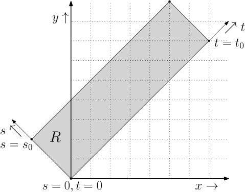
Figure 1. Diagonal coordinate system with diagonal rectangle $R$

Denote by $\mathcal{L}\big{(}(t_{1},s_{1}),(t_{2},s_{2})\big{)}$ the collection of LIPs between points $(t_{1},s_{1})$ and $(t_{2},s_{2})$ in the $t$–$s$ plane. The length of, that is the number of points on, any LIP in this collection is denoted by $L\big{(}(t_{1},s_{1}),(t_{2},s_{2})\big{)}$ and its expectation by $E\big{(}(t_{1},s_{1}),(t_{2},s_{2})\big{)}$. For a fixed domain $R$ (e.g. a diagonal rectangle), $\mathcal{L}^{R}\big{(}(t_{1},s_{1}),(t_{2},s_{2})\big{)}$ will denote the collection of LIPs between $(t_{1},s_{1})$ and $(t_{2},s_{2})$ constrained to lie within the domain $R$. We will use the notation $L^{R}\big{(}(t_{1},s_{1}),(t_{2},s_{2})\big{)}$ for the corresponding length and $E^{R}\big{(}(t_{1},s_{1}),(t_{2},s_{2})\big{)}$ for the expectation of this length. We write $L^{R}$ to denote the length of the LIP in $R$ when allowing arbitrary initial and end points in $R$. We shall use the shorthand

$$\begin{split}L_{t}&:=L\big{(}(0,0),(t,0)\big{)}\qquad\text{ and }\qquad L_{t,s}:=L\big{(}(0,0),(t,s)\big{)}.\end{split}$$

Note that $L_{t,s}=0$ if $|s|>t$ and $L_{t,s}$ equals $L_{\sqrt{t^{2}-s^{2}}}$ in distribution when $|s|\leqslant t$, since the area of the rectangle determines the distribution of the length of the LIP (by applying a linear transformation to the Poisson process). Correspondingly, we set

$$\begin{split}E_{t}:=\operatorname{\mathds{E}}L_{t}\qquad&\text{and}\qquad E_{t,s}:=\operatorname{\mathds{E}}L_{t,s}\,,\\ \sigma_{t}:=\sqrt{\operatorname{Var}(L_{t})}\qquad&\text{and}\qquad\sigma_{t,s}:=\sqrt{\operatorname{Var}(L_{t,s})}\,.\end{split}$$

Consider now a diagonal rectangle $R$ of length $\ell$ and width $w$. The following theorem gives bounds on the expectation of $L^{R}$. The first assertion in (4) follows as a consequence.

Theorem 1.2.

Fix $0<\delta<1/6$. Consider a diagonal rectangle $R$ of length $\ell$ and width $w$ such that $w(\log w)^{\frac{5}{3}}\leqslant\ell^{\frac{2}{3}}$. There exist constants $c(\delta),\,C(\delta)$ depending only on $\delta$ such that for $w$ large enough

$$\sqrt{2}\ell-C(\delta)\cdot(\log w)^{\frac{1}{3}+\delta}\cdot\frac{\ell}{w}\leqslant\operatorname{\mathds{E}}L^{R}\leqslant\sqrt{2}\ell-\frac{c(\delta)}{(\log w)^{\frac{5}{3}-\delta}}\cdot\frac{\ell}{w}$$ (6)

The first term $\sqrt{2}\ell$ matches the leading term in the expectation of the length of the unrestricted LIP in square domains. Our next result is a lower bound on the variance of $L^{R}$.

Theorem 1.3.

Consider a diagonal rectangle $R$ of length $\ell$ and width $w$ with $\frac{w}{\log\log w}\leqslant\ell^{\frac{2}{3}}$. There exists an $\epsilon_{0}>0$ such that for any $0<\epsilon<\epsilon_{0}$, we have

$$\operatorname{Var}(L^{R})\geqslant\left(\frac{\ell}{w^{\frac{1}{2}}}\right)^{1-\varepsilon}$$

for $w$ large enough.

Complementing this result, we provide upper bounds for all centered moments of $L^{R}$. These two theorems together prove the second assertion in (4).

Theorem 1.4.

Consider a diagonal rectangle $R$ of length $\ell$ and width $w$ such that $\frac{w}{(\log w)^{1/2}}\leqslant\ell^{\frac{2}{3}}$. For each fixed $k\geqslant 1$, there exists a constant $C(k)$ depending only on $k$ such that for $w$ large enough

$$\left\|L^{R}-\operatorname{\mathds{E}}L^{R}\right\|_{2k}\leqslant C(k)\cdot\frac{\ell^{\frac{1}{2}}}{w^{\frac{1}{4}}}\cdot(\log w)^{1+k},$$

where we use the notation $\|X\|_{p}:=(\operatorname{\mathds{E}}X^{p})^{1/p}$.

The theorems above suggest that the variance decreases as the width increases for each fixed $\ell$. It is worth noting that such a monotonicity property was a key (unproven) assumption made in the paper [18] for first passage percolation. Our final theorem is a Gaussian limit theorem for $L^{R}$ when the width is less than the critical width.

Theorem 1.5.

Fix $\gamma<\frac{2}{3}$. Consider a sequence of diagonal rectangles $R=R(\ell)$ of length $\ell$ and width $w(\ell)$ such that $w(\ell)\leqslant\ell^{\gamma}$. Then, as $\ell\to\infty$:

$$\frac{L^{R}-\operatorname{\mathds{E}}L^{R}}{\sqrt{\operatorname{Var}\,L^{R}}}\Rightarrow N(0,1).$$ (7)

Remark 1.1.

In the above results we have considered $L^{R}$, the length of the LIP within the rectangle $R$. One can also obtain similar results for $L^{R}(\mathbf{a},\mathbf{b})$, the length of the LIP among paths starting at $\mathbf{a}$, ending at $\mathbf{b}$ and restricted to lie within $R$, where $\mathbf{a},\mathbf{b}$ are points on the left and right boundaries of the rectangle $R$. This can be done by arguing as in the proof of Theorem 1.1 given in Section 9.

Remark 1.2.

The main ingredients in our results are the tail estimates in Lemma 2.2 and Lemma 2.5. We believe that results of a similar flavor hold for other models where corresponding estimates are known.

We now describe the outline of the paper. Section 2 describes the moderate deviation results as well as the van-den-Berg-Kesten type inequality that our analysis relies upon, and collects several consequences. Section 3 gives a lower bound on the expectation of the length of the LIP in diagonal rectangles and Section 4 provides error estimates for the length of the LIP in short blocks. We next prove Theorem 1.2 in Section 5. Section 6 contains the main argument of the paper in which we give a lower bound on the probability that LIPs (between arbitrary starting and ending points on the left and right boundaries respectively) in each block meet at a point. We use this result to prove Theorem 1.3 in Section 7. After this we prove Theorem 1.4 in Section 8 and then Theorem 1.5 in Section 9. We end the paper with a few open questions for the reader.

Throughout the article, $c,C$ will be used to denote arbitrary positive constants which may change from line to line. If the constants depend on a certain parameter this shall be indicated in parenthesis.

A remark on timing

A preliminary version of this paper containing full statements and proofs of the above results is available since December 2015 on the website of the first author. The second author presented these results at seminars in Bristol, Oxford and Sussex in 2015–16 while the third author discussed these at the June 2015 “Groups, Graphs and Stochastic Processes” Banff workshop. For various reasons, polishing of the draft and its final posting to the arXiv were greatly delayed, until its final appearance there on August 2018. In the interim, many results on last passage percolation, in the continuum and on the lattice have appeared, including [12, 11, 10, 9, 21, 22, 23, 24, 25]. Among these, especially related to the present work is a recent result of Basu, Ganguly and Hammond [10] who consider the length of the longest increasing path between $(0,0)$ and $(n,n)$, constrained to enclose an atypically large area of at least $(1/2+\alpha)n^{2}$. Apart from finding the law of large numbers for the model (in fact, they also find a limiting curve), the key result of their work is that the fluctuations around the limiting curve are of order $n^{1/2}$ and the convex hull facet length is of order $n^{3/4}$. This should be contrasted with the orders $n^{1/3}$ and $n^{2/3}$ for the unconstrained model. In a second related work which appeared very recently, Basu and Ganguly [9] find, among other results, upper and lower bounds on the variance of the last passage percolation time in thin cylinders which match up to a multiplicative constant. The latter two works kindly acknowledged our preprint.

2. Preliminaries

In this section we collect several results which we make use of in the sequel.

2.1. Asymptotic Behavior

The following was proved in [5].

Lemma 2.1.

There exist positive constants $c_{0},c_{1}$ such that

$$\sigma_{t} =c_{0}t^{1/3}\big{(}1+o(1)\big{)},$$ (8)

$$E_{t} =\sqrt{2}\,t-c_{1}t^{1/3}\big{(}1+o(1)\big{)}$$ (9)

as $t\to\infty$. We also have for all $k\geqslant 1$,

$$\big{\|}L_{t}-\sqrt{2}\,t\big{\|}_{k}\leqslant Ct^{1/3}.$$ (10)

for some constant $C>0$.

The next lemma gives tail bounds on the deviation of the length of the LIP from its mean. This lemma is the black box for our arguments and shall be referred to several times during the course of the paper. It collects results proved in [5], [29] and [30].

Lemma 2.2.

The following hold.

1. (Upper tail bounds) There exist constants $c,C>0$ such that for sufficiently large $t$,

   $$c\exp\big{(}-CT^{3/2}\big{)}\leqslant\operatorname{\mathds{P}}\left(\frac{L_{t}-E_{t}}{\sigma_{t}}\geqslant T\right)\leqslant C\exp\big{(}-cT^{3/2}\big{)}$$ (11)

   for all $1\leqslant T\leqslant t^{2/3}$.
   

2. (Lower tail bound) There exist constants $c,C>0$ such that for sufficiently large $t$,

   $$\operatorname{\mathds{P}}\left(\frac{L_{t}-E_{t}}{\sigma_{t}}\leqslant-T\right)\leqslant C\exp\big{(}-cT^{3}\big{)}$$ (12)

   for all $1\leqslant T\leqslant t^{2/3}$.

Proof.

The upper bounds in (11) and (12) have been proved in Lemma 7.1 of [5]; see also equations (1.4) and (1.5) in [27]. We now prove the lower bound in (11). From Lemma 2.1 and super-additivity of $E_{r}$, we have that

$$0\leqslant\frac{\sqrt{2}r-E_{r}}{\sigma_{r}}\leqslant a\text{ and }b_{1}\leqslant\frac{\sigma_{r}}{r^{1/3}}\leqslant b_{2}\text{ for all }r\geqslant 1$$

for some universal constants $a,b_{1},b_{2}>0$. From the distributional convergence of $2^{1/6}t^{-1/3}(L_{t}-\sqrt{2}t)$ to the Tracy-Widom disrtibution (see [5]) we note that there exists a number $\lambda>0$ such that

$$\operatorname{\mathds{P}}(L_{q}-E_{q}\geqslant k\sigma_{q})\geqslant e^{-\lambda}\quad\mbox{ for all }q\geqslant 1.$$

Let $k=\lceil a+{b_{2}}/{b_{1}}\rceil$ and choose $r=tT^{-3/2}\geqslant 1$ and now consider the event

$$A=\bigcap_{j=0}^{\lceil T^{3/2}\rceil}\Big{\{}L\big{(}(jr,0),((j+1)r,0)\big{)}-E_{r}\geqslant k\sigma_{r}\Big{\}}$$

The events in the braces are all independent and hence $\operatorname{\mathds{P}}(A)\geqslant e^{-\lambda(\lceil T^{3/2}\rceil+1)}$. Next note that on the event $A$, we have

$$\begin{split}L_{t}&\geqslant\sum_{j=0}^{\lceil T^{3/2}\rceil}L\big{(}(jr,0),((j+1)r,0)\big{)}\\ &\geqslant kT^{3/2}\sigma_{r}+T^{3/2}E_{r}\\ &\geqslant\Bigl{(}\frac{\sqrt{2}r-E_{r}}{\sigma_{r}}+\frac{b_{2}}{b_{1}}\Bigr{)}T^{3/2}\sigma_{r}+T^{3/2}E_{r}\\ &\geqslant\sqrt{2}rT^{3/2}+\frac{\sigma_{t}}{t^{1/3}}\cdot\frac{r^{1/3}}{\sigma_{r}}\cdot T^{3/2}\sigma_{r}=\sqrt{2}t+T\sigma_{t}\geqslant E_{t}+T\sigma_{t}.\end{split}$$

This completes the proof of the lemma. $\blacksquare$

The following fundamental lemma is a consequence of Lemma 2.1.

Lemma 2.3.

There exists a small $\alpha_{0}>0$ such that the following hold.

1. There exist positive constants $c,C$ such that whenever $|s|/t\leqslant\alpha_{0}$

   $$\frac{cs^{2}}{t}\leqslant E_{t}-E_{t,s}\leqslant\frac{Cs^{2}}{t}$$ (13)

2. There exist constants $c_{2},c_{3}>0$ such that whenever $|s|/t\leqslant\alpha_{0}$

   $$c_{2}t^{1/3}\leqslant\sigma_{t,s}\leqslant c_{3}t^{1/3}$$

   when $t$ is large enough. The upper bound holds for all $|s|\leqslant t$.

3. The tail bounds in Lemma 2.2 hold (perhaps with different constants) with $L_{t},E_{t},\sigma_{t}$ replaced by $L_{t,s},E_{t,s},\sigma_{t,s}$ respectively.

Proof.

The proof is a ready consequence of the distributional identity $L_{t,s}\stackrel{{\scriptstyle d}}{{=}}L_{\sqrt{t^{2}-s^{2}}}$ and the fact that $\sqrt{t^{2}-s^{2}}=t-\frac{s^{2}}{2t}(1+O(\frac{s^{2}}{t^{2}}))$ when $|s|\ll t$. $\blacksquare$

2.2. Transversal Fluctuations

In this section, we shall give a quantitative control on the transversal fluctuations of the LIP in square domains $[0,n]^{2}$. For this we shall discretize the space to a lattice of points of mesh size $1$. In order to show that the lengths of LIPs between points of the lattice are good approximations of the lengths of LIPs between general points we need a control over the number of Poisson points in small squares. Thus we define the event

$$A_{0}:=\left\{\text{The number of points in each $1\times 1$ square contained in $[0,n]^{2}$ is less than $(\log n)^{2}$}\right\}.$$

Lemma 2.4.

We have

$$\operatorname{\mathds{P}}\left(A_{0}^{c}\right)\leqslant C\exp\left(-c(\log n)^{2}\log\log n\right).$$

Proof.

It suffices to cover $[0,n]^{2}$ by $n^{2}$ squares of side-length $1$ and show that no such square contains more than $(\log n)^{2}/4$ Poisson points with high probability. This is because every square of side-length $1$ intersects at most $4$ of the $n^{2}$ squares. The number of Poisson points in a square of side-length $1$ is Poisson$(1)$ and hence the probability for it to be larger than $k$ is bounded by $\exp(-k\log k+k-1)$, yielding the lemma. $\blacksquare$

Let $S$ denote the maximal absolute value of the $s$ coordinate of a point on a maximizing path connecting $(0,0)$ to $(n,0)$ (in the $t$–$s$ plane). More precisely,

$$S=\max\left\{|\omega(t)|:0\leqslant t\leqslant n,\,t\mapsto\omega(t)\text{ is a maximizing path in }\mathcal{L}\big{(}(0,0),(n,0)\big{)}\right\}$$

Thus $S$ measures the transversal fluctuations of the path.

Lemma 2.5.

(Transversal fluctuations upper bound) For every $0<\delta<\frac{1}{3}$ there exits a positive integer $n_{0}(\delta)$, such that for $n\geqslant n_{0}(\delta)$ we have

$$\operatorname{\mathds{P}}\left(S>n^{2/3}\left(\log n\right)^{\frac{1}{3}+\delta}\right)\leqslant C\exp\big{(}-c(\log n)^{1+3\delta}\big{)}.$$

Proof.

Assume the event $A_{0}$ occurs as the probability of $A_{0}^{c}$ is much smaller than the probability we are interested in. Put a lattice of side length $1$ inside the square with corner points $(0,0)$ and $(n,0)$. If $S>n^{2/3}\left(\log n\right)^{\frac{1}{3}+\delta}$ there exists a point $(t,s)$ of the lattice with $\big{|}|s|-n^{2/3}\left(\log n\right)^{\frac{1}{3}+\delta}\big{|}\leqslant 1$ such that

$$L((0,0),(n,0))\leqslant L((0,0),(t,s))+L((t,s),(n,0))+(\log n)^{2}.$$

However, for each such $(t,s)$

$$\begin{split}E_{n}-E_{t,s}-E_{n-t,-s}&=(E_{n}-E_{t}-E_{n-t})+(E_{t}-E_{t,s})+(E_{n-t}-E_{n-t,-s})\end{split}$$

The first term in parenthesis on the right is of order $n^{1/3}$. The second and third terms in paranthesis are clearly nonnegative. When $|s|/t\leqslant\alpha_{0}$ (the constant appearing in Lemma 2.3) we have by (13) that $E_{t}-E_{t,s}\geqslant\frac{cs^{2}}{t}$. On the other hand when $|s|/t>\alpha_{0}$ we have $|s|/(n-t)\leqslant\alpha_{0}$ and therefore $E_{n-t}-E_{n-t,-s}\geqslant\frac{cs^{2}}{n-t}$. In either case we obtain

$$E_{n}-E_{t,s}-E_{n-t,-s}\geqslant cn^{1/3}(\log n)^{2/3+2\delta}$$ (14)

since $\big{|}|s|-n^{2/3}\left(\log n\right)^{\frac{1}{3}+\delta}\big{|}\leqslant 1$. The standard deviations of $\sigma_{n},\sigma_{t,s}$ and $\sigma_{n-t,-s}$ are all of order at most $n^{1/3}$. Thus, by (11), (12) and similar bounds in Lemma 2.3 it follows that

$$\begin{split}&\operatorname{\mathds{P}}\left(L((0,0),(n,0))\leqslant L((0,0),(t,s))+L((t,s),(n,0))+(\log n)^{2}\right)\\ &\leqslant\operatorname{\mathds{P}}\left(|L_{t,s}-E_{t,s}|>cn^{1/3}(\log n)^{2/3+2\delta}\right)+\operatorname{\mathds{P}}\left(|L_{n-t,-s}-E_{n-t,-s}|>cn^{1/3}(\log n)^{2/3+2\delta}\right)\\ &\qquad\qquad\qquad+\operatorname{\mathds{P}}\left(|L_{n}-E_{n}|>cn^{1/3}(\log n)^{2/3+2\delta}\right)\\ &\leqslant C\exp\big{(}-c(\log n)^{1+3\delta}\big{)}.\end{split}$$

Therefore the probability that a maximal path from $(0,0)$ to $(n,0)$ passes at distance $1$ from the lattice point $(t,s)$ is at most $C\exp(-c(\log n)^{1+3\delta})$. As there are less than $Cn^{2}$ points in our lattice, the lemma follows. $\blacksquare$

The following definition will be useful for us. It simplifies the exposition considerably.

Definition 2.1.

We say an event $A$ depending on the points in $\big{[}0,n]^{2}$ occurs with “overwhelming probability” if there is a $\theta>0$ such that

$$\operatorname{\mathds{P}}(A^{c})\leqslant\exp\big{(}-c(\log n)^{1+\theta}\big{)}.$$

In particular the event $\{S\leqslant n^{\frac{2}{3}}(\log n)^{\frac{1}{3}+\delta}\}$ occurs with overwhelming probability. A consequence of the above definition which we shall use several times without explicitly referring to is

Lemma 2.6.

Let the event $A$ depending on the points in $\big{[}0,n\big{]}^{2}$ occur with overwhelming probability. Then for every $\varepsilon>0$ and $k\geqslant 1$

$$\big{\|}L_{\sqrt{2}n}\cdot\mathds{1}_{A^{c}}\big{\|}_{k}\leqslant n^{\varepsilon}$$

for $n$ large enough.

Proof.

Let $K_{n}$ be the number of Poisson points in $[0,n]^{2}$. The following follows from a union bound by splitting the square into squares of side length $1$.

$$\begin{split}\operatorname{\mathds{P}}\big{(}L_{\sqrt{2}n}\geqslant m\big{)}&\leqslant\operatorname{\mathds{P}}\big{(}K_{n}\geqslant m\big{)}\\ &\leqslant n^{2}\operatorname{\mathds{P}}\Big{(}\text{Poisson}(1)>\frac{m}{n^{2}}\Big{)}\leqslant\exp\Big{(}-\frac{m}{n^{2}}\cdot\log\left(\frac{m}{n^{2}}\right)\Big{)}\end{split}$$

Therefore

$$\begin{split}\operatorname{\mathds{E}}\big{(}L_{\sqrt{2}n}^{k}\cdot\mathds{1}_{A^{c}}\big{)}&\leqslant\sum_{m\leqslant n^{3}}n^{3k}\operatorname{\mathds{E}}\big{(}\mathds{1}_{A^{c}}\cdot\mathds{1}\{L_{\sqrt{2}n}\leqslant n^{3}\}\big{)}\\ &\qquad+\sum_{i=1}^{\infty}n^{3(i+1)k}\operatorname{\mathds{E}}\big{(}\mathds{1}_{A^{c}}\cdot\mathds{1}\{in^{3}\leqslant L_{\sqrt{2}n}\leqslant(i+1)n^{3}\}\big{)}\end{split}$$

which is smaller than $n^{\varepsilon}$ when $n$ is large enough, since $A$ occurs with overwhelming probability and we have a fast decay in the tail probabilities of $L_{\sqrt{2}n}$ from Lemma 2.2. We will leave the details of this computation to the interested reader. $\blacksquare$

2.3. BK inequality

We now state a generalization of the classical BK inequality in site percolation suitable for our case. Denote by $\Omega$ the collection of all realizations $\omega$ of the Poisson point process on $\mathbb{R}_{+}^{2}$. We denote $\omega\subseteq\omega^{\prime}$ if all the Poisson points in $\omega$ are also present in $\omega^{\prime}$ and $\omega^{\prime}\backslash\omega$ will then be the realization with all the points in $\omega$ removed. For a subset $K\subseteq\mathbb{R}_{+}^{2}$ we denote $\omega_{K}$ to be the realization containing only the points of $\omega$ in $K$. A set $A\subseteq\Omega$ is increasing if $\omega\in A$ implies $\omega^{\prime}\in A$ when $\omega\subseteq\omega^{\prime}$. For increasing sets $A$ and $B$ define the disjoint occurence

$$\begin{split}A\Box B&=\{\omega:\text{there exist disjoint regions }K,\,L\subseteq\mathbb{R}_{+}^{2}\text{ such that }\omega_{K}\in A\text{ and }\omega_{L}\in B\}\\ &=\{\omega:\text{there exists }\omega^{\prime}\subseteq\omega\text{ such that }\omega^{\prime}\in A\text{ and }\omega\backslash\omega^{\prime}\in B\}.\end{split}$$

We then have

Lemma 2.7.

[38] For increasing events $A,B\subseteq\Omega$,

$$\operatorname{\mathds{P}}(A\Box B)\leqslant\operatorname{\mathds{P}}(A)\cdot\operatorname{\mathds{P}}(B).$$

3. Lower Bound of Expectation in Blocks

Consider the diagonal rectangle $R$ of length $\ell$ and width $w$. Consider two points $(0,a)$ and $(\ell,b)$ on opposite sides of the rectangle. Recall that $E^{R}\big{[}(0,a),(\ell,b)\big{]}=\operatorname{\mathds{E}}L^{R}\big{(}(0,a),(\ell,b)\big{)}$ is the expected value of the restricted LIP between the points $(0,a)$ and $(\ell,b)$. The following proposition shows that $E^{R}\big{[}(0,a),(\ell,b)\big{]}$ is not very far from $E_{\ell}$.

Proposition 3.1.

Fix $0<\delta<\frac{1}{3}$ and let $\ell^{\frac{2}{3}}(\log\ell)^{\frac{1}{3}+\delta}\leqslant w\leqslant\alpha_{0}\ell$ with $\ell$ large enough and $\alpha_{0}$ as in Lemma 2.3. There exists a constant $\mathcal{C}=\mathcal{C}(\delta)$ such that for any $0\leqslant a,b\leqslant w$,

$$E_{\ell}-\mathcal{C}\frac{w^{2}}{\ell}\leqslant E^{R}\big{[}(0,a),(\ell,b)\big{]}\leqslant E_{\ell}.$$

Proof.

The second inequality is immediate so let us consider the first inequality. It is sufficient to show that

$$E^{R}\big{[}(0,a),\big{(}\ell/2,w/2\big{)}\big{]}\geqslant E_{\frac{\ell}{2}}-C\frac{w^{2}}{\ell}.$$

because by symmetry we have a similar relation for $E^{R}\big{[}\big{(}\ell/2,w/2\big{)},\big{(}\ell,b\big{)}\big{]}$. We shall prove this with $a=0$ and indicate at the end how to modify the argument for general $a$. We shall consider paths which enter the interior of $R$ via successively larger rectangles such that the paths in each sub rectangle behave just like unrestricted paths. We make this precise as follows. Let

$$t_{0}=s_{0}=\ell^{1/3}.$$

We now define recursively two sequences

$$\begin{split}s_{k+1}&=2s_{k},\\ t_{k+1}&=t_{k}+\frac{s_{k}^{3/2}\ell}{2w^{3/2}}.\end{split}$$

Choose $k_{0}=O\big{(}\log_{2}(w/\ell^{1/3})\big{)}$ so that $s_{k_{0}}\leqslant\frac{w}{2}<s_{k_{0}+1}$. For this $k_{0}$ one can see that $\frac{\ell}{12}\leqslant t_{k_{0}}\leqslant\frac{\ell}{3}$ because

$$t_{k_{0}}=\ell^{1/3}+\frac{\ell^{3/2}}{2w^{3/2}}\left[1+2^{3/2}+2^{2\cdot 3/2}+\cdots+2^{(k_{0}-1)\cdot 3/2}\right]$$

Figure 2. Construction of the restricted path.

We now create an increasing (restricted to $R$) path from $(0,0)$ to $(\ell/2,w/2)$ by first moving directly to $(t_{0},s_{0})$ (not passing through any Poisson points) and then for each $0\leqslant k<k_{0}$, taking a LIP in $R$ from $(t_{k},s_{k})$ to $(t_{k+1},s_{k+1})$. By using the transversal fluctuation Lemma 2.5, as $t_{k+1}-t_{k}$ is short compared with $s_{k}$, we may treat each such LIP as an unrestricted LIP (not constrained to lie in $R$) as the unrestricted and restricted LIP coincide with overwhelming probability. In the last step we take a LIP in $R$ from $(t_{k_{0}},s_{k_{0}})$ to $(\ell/2,w/2)$ which again coincides with the unrestricted LIP with overwhelming probability. In particular one can show that

$$\big{|}E^{R}\big{(}(t_{k},s_{k}),(t_{k+1},s_{k+1})\big{)}-E\big{(}(t_{k},s_{k}),(t_{k+1},s_{k+1})\big{)}\big{|}\leqslant\ell^{1/6}$$ (15)

and

$$\Big{|}E^{R}\big{(}(t_{k_{0}},s_{k_{0}}),(\ell/2,w/2)\big{)}-E\big{(}(t_{k_{0}},s_{k_{0}}),(\ell/2,w/2)\big{)}\Big{|}\leqslant\ell^{1/6}.$$ (16)

Let us show the first inequality (15) above and leave the second (16) to the reader.

$$\begin{split}&\big{|}E^{R}\big{(}(t_{k},s_{k}),(t_{k+1},s_{k+1})\big{)}-E\big{(}(t_{k},s_{k}),(t_{k+1},s_{k+1})\big{)}\big{|}\\ &\leqslant 2\operatorname{\mathds{E}}\left[L\big{(}(t_{k},s_{k}),\,(t_{k+1},s_{k+1})\big{)}\cdot\mathds{1}\{\text{path goes out of the rectangle with endpoints }(t_{k},s_{k}),\,(t_{k+1},s_{k+1})\}\right]\\ &\leqslant 2\ell\cdot\operatorname{\mathds{P}}\left(\{\text{path goes out of the rectangle with endpoints }(t_{k},s_{k}),\,(t_{k+1},s_{k+1})\}\right)\\ &\qquad+\sum_{i=0}^{\infty}(2\ell+i\ell^{1/3})\cdot\operatorname{\mathds{P}}\left(2\ell+i\ell^{1/3}\leqslant L\big{(}(t_{k},s_{k}),\,(t_{k+1},s_{k+1})\big{)}\leqslant 2\ell+(i+1)\ell^{1/3}\right).\end{split}$$

Thanks to the tail bounds in Lemma 2.2 and the bound on the probability of large transversal fluctuations in Lemma 2.5, the inequality (15) follows for all large $\ell$.

Since the maximal restricted path in $R$ has larger length than the length of the path obtained from our construction we get, using Lemma 2.3

$$\begin{split}&E_{\frac{\ell}{2}}-E^{R}\big{[}(0,a),(\ell/2,w/2)\big{]}\\ &\quad\leqslant E_{\frac{\ell}{2}}-\sum_{k=0}^{k_{0}-1}E\big{(}(t_{k},s_{k}),(t_{k+1},s_{k+1})\big{)}-E\big{(}(t_{k_{0}},s_{k_{0}}),(\ell/2,w/2)\big{)}+C\ell^{1/6}k_{0}\\ &\quad\leqslant E_{\frac{\ell}{2}}-\sum_{k=0}^{k_{0}-1}\Big{[}E_{t_{k+1}-t_{k}}-C\frac{(s_{k+1}-s_{k})^{2}}{t_{k+1}-t_{k}}\Big{]}-\Big{[}E_{\frac{\ell}{2}-t_{k_{0}}}-C\frac{(w/2)^{2}}{\frac{\ell}{2}-t_{k_{0}}}\Big{]}+C\ell^{1/6}k_{0}\\ &\quad\leqslant E_{\frac{\ell}{2}}-\sum_{k=0}^{k_{0}-1}E_{t_{k+1}-t_{k}}-E_{\frac{\ell}{2}-t_{k_{0}}}+C\Big{[}\sum_{k=0}^{k_{0}-1}\frac{(s_{k+1}-s_{k})^{2}}{t_{k+1}-t_{k}}+\frac{(w/2)^{2}}{\frac{\ell}{2}-t_{k_{0}}}\Big{]}+C\ell^{1/6}k_{0}\\ &\quad\leqslant C\ell^{1/3}+C\sum_{k=0}^{k_{0}-1}\Big{\{}\frac{s_{k}^{3/2}\ell}{2w^{3/2}}\Big{\}}^{1/3}+C\Big{[}\sum_{k=0}^{k_{0}-1}\frac{s_{k}^{2}}{s_{k}^{3/2}\ell/2w^{3/2}}+C\frac{w^{2}}{\ell}\Big{]}+C\ell^{1/6}k_{0}\\ &\quad\leqslant C\ell^{1/3}+\frac{C\ell^{1/3}}{2^{1/3}w^{1/2}}\sum_{k=0}^{k_{0}-1}2^{k/2}\ell^{1/6}+C\sum_{k=0}^{k_{0}-1}\frac{2^{k/2}\ell^{1/6}w^{3/2}}{\ell}+C\frac{w^{2}}{\ell}+C\ell^{1/6}k_{0}\\ &\quad\leqslant C\frac{w^{2}}{\ell}.\end{split}$$

We have used the bound to $2^{k_{0}/2}\leqslant w^{1/2}/\ell^{1/6}$ to arrive at the final step.

Now we explain how the argument can be extended for any $a$. For $a\leqslant\ell^{1/3}$, we follow the same rectangles. For $\ell^{1/3}<a\leqslant w/2$ and $s_{i}<a\leqslant s_{i+1}$, we take the maximal path to $(t_{i+1},s_{i+1})$ (which will remain in $R$ with overwhelming probability) and then follow the remaining rectangles. The argument for $a\geqslant w/2$ follows along the same lines by symmetry. $\blacksquare$

4. Upper bounds in blocks

Consider a diagonal rectangle $R$ of width $w$ and length $\ell$. Let

$$\Delta(R):=\max_{\mathbf{x}\in B_{l},\,\mathbf{y}\in B_{r}}L^{R}(\mathbf{x},\mathbf{y})-\min_{\mathbf{x}\in B_{l},\,\mathbf{y}\in B_{r}}L^{R}(\mathbf{x},\mathbf{y}).$$ (17)

Here $B_{l},\,B_{r}$ are the left and right boundaries of $R$.

Proposition 4.1.

Fix $k\geqslant 1$ and $0<\delta<\frac{1}{3}$ and let $\ell^{\frac{2}{3}}(\log\ell)^{\frac{1}{3}+\delta}\leqslant w\leqslant\alpha_{0}\ell$ with $\alpha_{0}$ as in Lemma 2.3. There exists a constant $C=C(\delta,k)$ such that

$$\left\|\Delta(R)\right\|_{k}\leqslant C\frac{w^{2}}{\ell}$$

for large enough $\ell$.

Proof.

We first bound $\Delta(R)$ as follows.

$$\begin{split}\Delta(R)&\leqslant\max_{\mathbf{x}\in B_{l},\,\mathbf{y}\in B_{r}}\big{[}L(\mathbf{x},\mathbf{y})-\operatorname{\mathds{E}}L(\mathbf{x},\mathbf{y})\big{]}+\left[\max_{\mathbf{x}\in B_{l},\,\mathbf{y}\in B_{r}}\operatorname{\mathds{E}}L(\mathbf{x},\mathbf{y})-\min_{\mathbf{x}\in B_{l},\,\mathbf{y}\in B_{r}}\operatorname{\mathds{E}}L(\mathbf{x},\mathbf{y})\right]\\ &\qquad-\min_{\mathbf{x}\in B_{l},\,\mathbf{y}\in B_{r}}\big{[}L^{R}(\mathbf{x},\mathbf{y})-\operatorname{\mathds{E}}L(\mathbf{x},\mathbf{y})\big{]}\\ &\leqslant\max_{\mathbf{x}\in B_{l},\,\mathbf{y}\in B_{r}}\big{[}L(\mathbf{x},\mathbf{y})-\operatorname{\mathds{E}}L(\mathbf{x},\mathbf{y})\big{]}+\left[\max_{\mathbf{x}\in B_{l},\,\mathbf{y}\in B_{r}}\operatorname{\mathds{E}}L(\mathbf{x},\mathbf{y})-\min_{\mathbf{x}\in B_{l},\,\mathbf{y}\in B_{r}}\operatorname{\mathds{E}}L(\mathbf{x},\mathbf{y})\right]\\ &\qquad-\min_{\mathbf{x}\in B_{l},\,\mathbf{y}\in B_{r}}\big{[}\tilde{L}^{R}(\mathbf{x},\mathbf{y})-\operatorname{\mathds{E}}L(\mathbf{x},\mathbf{y})\big{]}\end{split}$$ (18)

where $\tilde{L}^{R}(\mathbf{x},\mathbf{y})$ are restricted paths from $\mathbf{x}$ to $\mathbf{y}$ passing through the sub-rectangles constructed as in Proposition 3.1. By Lemma 2.3,

$$\left[\max_{\mathbf{x}\in B_{l},\,\mathbf{y}\in B_{r}}\operatorname{\mathds{E}}L(\mathbf{x},\mathbf{y})-\min_{\mathbf{x}\in B_{l},\,\mathbf{y}\in B_{r}}\operatorname{\mathds{E}}L(\mathbf{x},\mathbf{y})\right]\leqslant C\frac{w^{2}}{\ell}.$$

Let us next look at the first term on the right hand side of (18). We divide both $B_{l}$ and $B_{r}$ into intervals of length $\ell^{-1}$. Let $\mathbf{a}_{0},\,\mathbf{a}_{1},\cdots,\mathbf{a}_{[w\ell]}$ denote the partition points on the left boundary and let $\mathbf{b}_{0},\,\mathbf{b}_{1},\cdots,\mathbf{b}_{[w\ell]}$ denote the partition points on the right boundary. We claim that

$$\Big{\|}\max_{\mathbf{x}\in B_{l},\,\mathbf{y}\in B_{r}}\big{[}L(\mathbf{x},\mathbf{y})-\operatorname{\mathds{E}}L(\mathbf{x},\mathbf{y})\big{]}\Big{\|}_{k}\leqslant\Big{\|}\max_{i,j}\big{[}L(\mathbf{a}_{i},\mathbf{b}_{j})-\operatorname{\mathds{E}}L(\mathbf{a}_{i},\mathbf{b}_{j})\big{]}\Big{\|}_{k}+C(k)\frac{w^{2}}{\ell}.$$

This is because with overwhelming probability the number of points in each rectangle with vertices $\mathbf{a}_{i},\mathbf{a}_{i+1},\mathbf{b}_{j},\mathbf{b}_{j+1}$ is at most $(\log\ell)^{2}$. An application of the tail bounds in Lemma 2.3 along with a union bound gives

$$\operatorname{\mathds{P}}\left(\left|L(\mathbf{a}_{i},\mathbf{b}_{j})-\operatorname{\mathds{E}}L(\mathbf{a}_{i},\mathbf{b}_{j})\right|>\ell^{\frac{1}{3}}(\log\ell)^{\frac{2}{3}+2\delta}\text{ for some }i,j\right)\leqslant\exp\big{(}-c(\log\ell)^{1+3\delta}\big{)}.$$ (19)

From this it follows that

$$\Big{\|}\max_{i,j}\big{[}L(\mathbf{a}_{i},\mathbf{b}_{j})-\operatorname{\mathds{E}}L(\mathbf{a}_{i},\mathbf{b}_{j})\big{]}\Big{\|}_{k}\leqslant C(\delta,k)\cdot\ell^{\frac{1}{3}}(\log\ell)^{\frac{2}{3}+2\delta}\leqslant C(\delta,k)\frac{w^{2}}{\ell}$$

which bounds the first term in (18). Now we proceed to the last term in (18). The $k$th norm is bounded by

$$\begin{split}&\leqslant\Big{\|}\max_{\mathbf{x},\mathbf{y}}\big{|}\tilde{L}^{R}(\mathbf{x},\mathbf{y})-\operatorname{\mathds{E}}\tilde{L}^{R}(\mathbf{x},\mathbf{y})\big{|}\Big{\|}_{k}+\max_{\mathbf{x},\mathbf{y}}\big{|}\operatorname{\mathds{E}}\tilde{L}^{R}(\mathbf{x},\mathbf{y})-\operatorname{\mathds{E}}L(\mathbf{x},\mathbf{y})\big{|}\\ &=\Big{\|}\max_{i,j}\big{|}\tilde{L}^{R}(\mathbf{a}_{i},\mathbf{b}_{j})-\operatorname{\mathds{E}}\tilde{L}^{R}(\mathbf{a}_{i},\mathbf{b}_{j})\big{|}\Big{\|}_{k}+\max_{\mathbf{x},\mathbf{y}}\big{|}\operatorname{\mathds{E}}\tilde{L}^{R}(\mathbf{x},\mathbf{y})-\operatorname{\mathds{E}}L(\mathbf{x},\mathbf{y})\big{|}\\ &\leqslant\Big{\|}\max_{i,j}\big{|}\tilde{L}^{R}(\mathbf{a}_{i},\mathbf{b}_{j})-\operatorname{\mathds{E}}\tilde{L}^{R}(\mathbf{a}_{i},\mathbf{b}_{j})\big{|}\Big{\|}_{k}+C(\delta,k)\frac{w^{2}}{\ell}\leqslant C(\delta,k)\frac{w^{2}}{\ell}.\end{split}$$

The second last inequality follows by an application of Proposition 3.1. Since the number of rectangles in the construction of Proposition 3.1 is $O(\log(w/\ell^{1/3}))$ and the behavior of the path in each sub-rectangle is unrestricted, we can use a bound similar to (19) to conclude the last inequality. $\blacksquare$

We next give a bound on the $k$th centered moments of

$$L^{R}:=\max_{\mathbf{x}\in B_{l},\,\mathbf{y}\in B_{r}}L^{R}(\mathbf{x},\mathbf{y}).$$

Lemma 4.2.

Fix $k\geqslant 1$ and $0<\delta<\frac{1}{3}$ and let $\ell^{\frac{2}{3}}(\log\ell)^{\frac{1}{3}+\delta}\leqslant w\leqslant\alpha_{0}\ell$ with $\alpha_{0}$ as in Lemma 2.3. There exists a constant $C=C(\delta,k)$ such that

$$\big{\|}L^{R}-\operatorname{\mathds{E}}L^{R}\big{\|}_{k}\leqslant C\frac{w^{2}}{\ell}.$$

for large enough $\ell$.

Proof.

We write

$$\begin{split}L^{R}-\operatorname{\mathds{E}}L^{R}&=\big{[}L^{R}-L^{R}\big{(}(0,w/2),(\ell,w/2)\big{)}\big{]}+\big{[}L^{R}\big{(}(0,w/2),(\ell,w/2)\big{)}-\operatorname{\mathds{E}}L^{R}\big{(}(0,w/2),(\ell,w/2)\big{)}\big{]}\\ &\hskip 85.35826pt+\big{[}\operatorname{\mathds{E}}L^{R}\big{(}(0,w/2),(\ell,w/2)\big{)}-\operatorname{\mathds{E}}L^{R}\big{]}\end{split}$$ (20)

An application of Proposition 4.1 gives us that

$$\begin{split}\big{\|}L^{R}-L^{R}\big{(}(0,w/2),(\ell,w/2)\big{)}\big{\|}_{k}&\leqslant\|\Delta(R)\|_{k}\leqslant C(\delta,k)\frac{w^{2}}{\ell}\\ \big{|}\operatorname{\mathds{E}}L^{R}-\operatorname{\mathds{E}}L^{R}\big{(}(0,w/2),(\ell,w/2)\big{)}\big{|}&\leqslant\|\Delta(R)\|_{k}\leqslant C(\delta,k)\frac{w^{2}}{\ell}\end{split}$$

As for the second term on the right hand side of (20) we observe by Lemma 2.5 that with overwhelming probability the maximal path from $(0,w/2)$ to $(\ell,w/2)$ lies within the rectangle $R$. Hence

$$\big{\|}L^{R}\big{(}(0,w/2),(\ell,w/2)\big{)}-\operatorname{\mathds{E}}L^{R}\big{(}(0,w/2),(\ell,w/2)\big{)}\big{\|}_{k}\leqslant C(\delta,k)\frac{w^{2}}{\ell}.$$

since the unrestricted LIP from $(0,w/2)$ to $(\ell,w/2)$ has moments of order $\ell^{1/3}$ by (10). This completes the proof of the lemma. $\blacksquare$

5. Proof of Theorem 1.2

Fix $0<\delta<\frac{1}{6}$. Let us consider the lower bound first. Choose $n$ so that $w=n^{\frac{2}{3}}(\log n)^{\frac{1}{3}+\delta}$. We divide $R$ into $m=\lfloor\ell/n\rfloor$ blocks of length $n$ and the final block of length smaller than $n$. For each of the blocks $R_{i}$, let $L^{R}_{i}$ denote the length of the restricted LIP from the midpoint of the left boundary to the midpoint of the right boundary. Note that by Lemma 2.5 the restricted LIP between the midpoints coincides with the unrestricted LIP with overwhelming probability. Thus

$$\operatorname{\mathds{E}}L^{R}_{i}=\sqrt{2}n-c_{1}n^{1/3}\big{(}1+o(1)\big{)},\;1\leqslant i\leqslant m$$

and similarly for the final block. One gets immediately

$$\operatorname{\mathds{E}}L^{R}\geqslant\sum_{i=1}^{m+1}\operatorname{\mathds{E}}L^{R}_{i}\geqslant\sqrt{2}\ell-C\cdot mn^{1/3}\geqslant\sqrt{2}\ell-C(\delta)\cdot(\log w)^{\frac{1}{3}+\delta}\cdot\frac{\ell}{w}.$$

Let us now turn to the upper bound in (6). For this we choose $n$ such that $n^{\frac{2}{3}}(\log n)^{\frac{1}{3}+\delta}\leqslant w\leqslant 2n^{\frac{2}{3}}(\log n)^{\frac{1}{3}+\delta}$ such that $\frac{\ell}{n(\log n)^{3}}$ is a positive integer. We provide some details on why we can choose such an $n$. It is easy to see that for any such $n$ we have that $n(\log n)^{3}\leqslant c(\delta)w^{\frac{3}{2}}(\log w)^{\frac{5}{2}-\frac{3\delta}{2}}\ll l$. For the exact divisibility first choose $n_{1}$ so that $w=2n_{1}^{\frac{2}{3}}(\log n_{1})^{\frac{1}{3}+\delta}$. When dividing $\ell$ by $n_{1}$ the remainder is at most $n_{1}(\log n_{1})^{3}$. It then follows that we can choose $n_{2}$ appropriately so that $n_{1}\leqslant n_{2}\leqslant 2n_{1}$ and $n_{2}(\log n_{2})^{3}$ exactly divides $\ell$. It is clear that $w\leqslant 2n_{2}^{\frac{2}{3}}(\log n_{2})^{\frac{1}{3}+\delta}$ and $w\geqslant 2(n_{2}/2)^{\frac{2}{3}}\big{(}\log(n_{2}/2)\big{)}^{\frac{1}{3}+\delta}\geqslant n_{2}^{\frac{2}{3}}(\log n_{2})^{\frac{1}{3}+\delta}$ when $w$ is large enough.

Let us therefore now assume that we have an $n$ such that $n^{\frac{2}{3}}(\log n)^{\frac{1}{3}+\delta}\leqslant w\leqslant 2n^{\frac{2}{3}}(\log n)^{\frac{1}{3}+\delta}$ and $n^{\prime}=n(\log n)^{3}$ exactly divides $\ell$. We split $R$ into $m^{\prime}=\ell/n^{\prime}$ blocks $R_{i}$ of length $n^{\prime}$. For each $1\leqslant i\leqslant m^{\prime}$ let $X_{i}$ denote the length of the restricted LIP in $R_{i}$ and let $L^{R}_{i}$ as before denote the length of the restricted (midpoint to midpoint) LIP. Divide $R_{i}$ further into three sub-rectangles $S_{i}^{(1)},\,S_{i}^{(2)},\,S_{i}^{(3)}$ where the $S$-rectangles on either side have length $n$ and $S_{i}^{(2)}$ has the remaining length. Denote by $Y_{i}$ the length of restricted LIP in $S_{i}^{(2)}$.

Figure 3. Division of block $R_{i}$

It is clear that

$$\begin{split}X_{i}&\leqslant\max_{\mathbf{x}_{1},\mathbf{y}_{1}}L^{R}(\mathbf{x}_{1},\mathbf{y}_{1})+Y_{i}+\max_{\mathbf{x}_{3},\mathbf{y}_{3}}L^{R}(\mathbf{x}_{3},\mathbf{y}_{3})\\ L^{R}_{i}&\geqslant\min_{\mathbf{x}_{1},\mathbf{y}_{1}}L^{R}(\mathbf{x}_{1},\mathbf{y}_{1})+Y_{i}+\min_{\mathbf{x}_{3},\mathbf{y}_{3}}L^{R}(\mathbf{x}_{3},\mathbf{y}_{3})\end{split}$$

where $\mathbf{x}_{1},\mathbf{y}_{1}$ are generic points on the left and right boundaries of $S_{i}^{(1)}$, and $\mathbf{x}_{3},\mathbf{y}_{3}$ are generic points on the left and right boundaries of $S_{i}^{(3)}$ . Therefore

$$\operatorname{\mathds{E}}|X_{i}-L^{R}_{i}|\leqslant 2\|\Delta\big{(}S_{i}^{(1)}\big{)}\|_{1}\leqslant C(\delta)\frac{w^{2}}{n}$$

by Proposition 4.1. This would then give

$$\operatorname{\mathds{E}}L^{R}\leqslant\sum_{i=1}^{m^{\prime}}\operatorname{\mathds{E}}X_{i}\leqslant\sum_{i=1}^{m^{\prime}}\big{(}\operatorname{\mathds{E}}L^{R}_{i}+C(\delta)\frac{w^{2}}{n}\big{)}.$$

We can bound $\operatorname{\mathds{E}}L^{R}_{i}$ by the expected value of the length of the unrestricted (midpoint to midpoint) LIP to get an upper bound of $\sqrt{2}n^{\prime}-c_{1}(n^{\prime})^{1/3}\big{(}1+o(1)\big{)}$ and thus

$$\operatorname{\mathds{E}}L^{R}\leqslant\sqrt{2}\ell-cm^{\prime}(n^{\prime})^{\frac{1}{3}}+C(\delta)\cdot m^{\prime}\frac{w^{2}}{n}\leqslant\sqrt{2}\ell-\frac{C(\delta)}{(\log n)^{\frac{5}{3}-\delta}}\cdot\frac{\ell}{w}.$$

This gives the required upper bound because $\log n$ is of the same order as $\log w$. $\blacksquare$

6. Meeting of Paths

Given $\delta,\delta^{\prime}>0$ and $n$ consider a diagonal rectangle $R$ of width $w^{(b)}=w^{(b)}(n)$ and length $\ell^{(b)}=\ell^{(b)}(n)$ with

$$w^{(b)}=n^{\frac{2}{3}}(\log n)^{\frac{1}{3}+\delta}.$$ (21)

and

$$\ell^{(b)}=n\big{[}\sqrt{\log n}\big{]}+2\tau\quad\text{where}\quad\tau:=\frac{n}{(\log n)^{\delta^{\prime}}}.$$ (22)

Rectangles of this type will form the basic blocks in Section 7. In this section we give a lower bound on the probability that LIPs between arbitrary starting and ending points within the blocks meet. This would help us get the necessary independence structure needed for getting a lower bound on the variance done in Section 7.

Denote by $\mathbf{a}$ a generic point on the left boundary of $R$ and by $\mathbf{b}$ a generic point on the right boundary of $R$. Define the event

$$\Omega:=\{\text{There exists $\mathbf{p}\in R$ such that for all $\mathbf{a},\,\mathbf{b}$ there is a path in $\mathcal{L}^{R}(\mathbf{a},\mathbf{b})$ passing through $\mathbf{p}$}\}.$$ (23)

By geometric considerations one observes that

$$\Omega=\{\text{A path in $\mathcal{L}^{R}\big{(}(0,0),(\ell^{(b)},0)\big{)}$ intersects a path in $\mathcal{L}^{R}\big{(}(0,w^{(b)}),(\ell^{(b)},w^{(b)})\big{)}$}\}.$$

In fact any point in the intersection of a path $\tilde{p}$ in $\mathcal{L}^{R}\big{(}(0,0),(\ell^{(b)},0)\big{)}$ and a path $\tilde{q}$ in $\mathcal{L}^{R}\big{(}(0,w^{(b)}),(\ell^{(b)},w^{(b)})\big{)}$ would be such a point $\mathbf{p}$. This is because from any path $\tilde{r}$ in $\mathcal{L}^{R}(\mathbf{a},\mathbf{b})$ which intersects either of these paths, one could construct another path in $\mathcal{L}^{R}(\mathbf{a},\mathbf{b})$ passing through the point $\mathbf{p}$. Note first that the path $\tilde{r}$ would either intersect $\tilde{p}$ or $\tilde{q}$ at least two points. Without loss of generality assume that it intersects $\tilde{p}$ at points $p_{1}$ (the first intersecting point) and $p_{2}$ (the last intersecting point). Construct another path following $\tilde{r}$ till $p_{1}$, then following $\tilde{p}$ from $p_{1}$ to $p_{2}$, and finally following $\tilde{r}$ from $p_{2}$ to $\mathbf{b}$. One can argue that the length of this new path between $p_{1}$ and $p_{2}$ is the same as the length of $\tilde{r}$ between $p_{1}$ and $p_{2}$. Having a greater length would be a contradiction to the maximality of $\tilde{r}$ while having a lower length would be a contradiction to the maximality of $\tilde{p}$.

Figure 4. Picture depicting $\Omega\text{ and }\mathbf{p}$

The following is the main result of the section.

Theorem 6.1.

Fix $\delta,\delta^{\prime}$ satisfying

$$\quad 0<\delta<\frac{1}{12}\quad\text{and}\quad 0<\delta^{\prime}<\frac{1}{6}-2\delta.$$ (24)

Let $R$ be a diagonal rectangle with length $\ell^{(b)}=\ell^{(b)}(n)$ and width $w^{(b)}=w^{(b)}(n)$ satisfying (21) and (22). Then for any $0<\epsilon<1$ we have

$$\operatorname{\mathds{P}}(\Omega)\geqslant n^{-\epsilon}$$ (25)

for all $n$ large enough.

Fix $0<\epsilon<1$ and $\delta,\delta^{\prime}$ satisfying (24). Define the following events.

$$\begin{split}A_{1}&:=\left\{L^{R}((0,0),(\ell^{(b)},0))\geqslant E_{\ell^{(b)}}+10\varepsilon^{\frac{2}{3}}n^{\frac{1}{3}}(\log n)^{\frac{5}{6}}\right\},\\ A_{1}^{\prime}&:=\left\{L^{R}((0,w^{(b)}),(\ell^{(b)},w^{(b)}))\geqslant E_{\ell^{(b)}}+\varepsilon^{\frac{2}{3}}n^{\frac{1}{3}}(\log n)^{\frac{5}{6}}\right\},\\ A_{2}&:=\left\{A_{1}^{\prime}\text{ does not occur disjointly from $A_{1}$}\right\}=\left(A_{1}\Box A_{1}^{\prime}\right)^{c}.\end{split}$$ (26)

Our approach to lower bound $\operatorname{\mathds{P}}(\Omega)$ proceeds by showing that $A_{1}$ has probability $n^{-c\varepsilon}$ and $A_{2}$ is likely given $A_{1}$. Under the event $A_{1}$, the LIP between the point $(0,0)$ and $(\ell^{(b)},0)$ is very long and the only potential way for $(0,w^{(b)})$ to be connected to $(\ell^{(b)},w^{(b)})$ via a path with similarly large length is by intersecting the first path. To make this more precise, we need also control the loss incurred in connecting a corner point of $R$ to a point near the central line of $R$ (with $s$ coordinate roughly $w^{(b)}/2$). To this end, define the events

$$\begin{split}A_{3}&:=\left\{\forall\,0\leqslant s\leqslant w^{(b)},\;\,L^{R}\big{(}(0,0),(\tau,s)\big{)}\leqslant E_{\tau}+n^{\frac{1}{3}}(\log n)^{\frac{2}{3}}\right\},\\ A_{4,s^{\prime}}&:=\left\{L^{R}\big{(}(0,0),(\tau,s^{\prime})\big{)}\geqslant E_{\tau}-2\mathcal{C}n^{\frac{1}{3}}(\log n)^{\frac{2}{3}+2\delta+\delta^{\prime}}\right\},\qquad 0\leqslant s^{\prime}\leqslant w^{(b)}\end{split}$$ (27)

and the symmetric events

$$\begin{split}A_{3}^{\prime}&:=\left\{\forall\,0\leqslant s\leqslant w^{(b)},\;\,L^{R}\big{(}(\ell^{(b)}-\tau,s),(\ell^{(b)},0)\big{)}\leqslant E_{\tau}+n^{\frac{1}{3}}(\log n)^{\frac{2}{3}}\right\}\\ A_{4,s^{\prime}}^{\prime}&:=\left\{L^{R}\big{(}(\ell^{(b)}-\tau,s^{\prime}),(\ell^{(b)},0)\big{)}\geqslant E_{\tau}-2\mathcal{C}n^{\frac{1}{3}}(\log n)^{\frac{2}{3}+2\delta+\delta^{\prime}}\right\},\qquad 0\leqslant s^{\prime}\leqslant w^{(b)}.\end{split}$$ (28)

where $\mathcal{C}=\mathcal{C}(\delta)$ is the constant appearing in Proposition 3.1. The following lemmas gather bounds which will be combined to prove Theorem 6.1.

Lemma 6.2.

There exists a constant $c>0$ independent of $\epsilon$ and $n_{0}=n_{0}(\delta,\delta^{\prime},\epsilon)$ such that for all $n\geqslant n_{0}$ we have

$$\operatorname{\mathds{P}}(A_{2}^{c}|A_{1})\leqslant n^{-c\varepsilon}.$$ (29)

Proof.

The estimate for $\operatorname{\mathds{P}}(A_{2}^{c}|A_{1})$ follows by an application of Lemma 2.7 and comparison with LIP which are not constrained to lie in $R$.

$$\operatorname{\mathds{P}}(A_{2}^{c}|A_{1})\leqslant\operatorname{\mathds{P}}(A_{1}^{\prime})\leqslant\operatorname{\mathds{P}}\big{(}L((0,w^{(b)}),(\ell^{(b)},w^{(b)}))\geqslant E_{\ell^{(b)}}+\varepsilon^{\frac{2}{3}}n^{\frac{1}{3}}(\log n)^{\frac{5}{6}}\big{)}\leqslant Cn^{-c\varepsilon},$$

the last inequality following from (8) and (11). $\blacksquare$

Lemma 6.3.

There exist constants $c,C>0$ and $n_{0}=n_{0}(\delta,\delta^{\prime})$ such that for all $n\geqslant n_{0}$ we have

$$\operatorname{\mathds{P}}(A_{3}^{c})\leqslant C\exp\big{(}-c(\log n)^{1+\frac{\delta^{\prime}}{2}}\big{)},$$ (30)

A similar bound as (30) holds for $\operatorname{\mathds{P}}\big{(}(A^{\prime}_{3})^{c}\big{)}$.

Proof.

As in Proposition 4.1 we might as well discretize the possible values of $s$ to only about $\tau w^{(b)}$ possible values at distance $\tau^{-1}$ apart; see the argument leading up to (19). For each value of $s$, we compare with the LIP which are not constrained to lie in $R$ to obtain

$$\begin{split}\operatorname{\mathds{P}}\big{[}L^{R}\big{(}(0,0),(\tau,s)\big{)}>E_{\tau}+n^{\frac{1}{3}}(\log n)^{\frac{2}{3}}\big{]}&\leqslant\operatorname{\mathds{P}}\big{[}L\big{(}(0,0),(\tau,s)\big{)}>E_{\tau}+n^{\frac{1}{3}}(\log n)^{\frac{2}{3}}\big{]}\\ &=\operatorname{\mathds{P}}\big{[}L\big{(}(0,0),(\tau,s)\big{)}>E_{\tau}+\tau^{\frac{1}{3}}(\log n)^{\frac{\delta^{\prime}}{3}}(\log n)^{\frac{2}{3}}\big{]}\\ &\leqslant C\exp\big{(}-c(\log n)^{1+\frac{\delta^{\prime}}{2}}\big{)},\end{split}$$

the last inequality following from Lemma 2.3. The lemma follows from a union bound. $\blacksquare$

Lemma 6.4.

For any $D>0$ and $0\leqslant s^{\prime}\leqslant w^{(b)}$ we have

$$\operatorname{\mathds{P}}(A_{4,s^{\prime}}^{c})=o(n^{-D}).$$ (31)

A similar bound as (31) holds for $\operatorname{\mathds{P}}\big{(}(A^{\prime}_{4,s^{\prime}})^{c}\big{)}$.

Proof.

The argument is based on the proof of Proposition 3.1 to which we shall refer. Fix $D>0$. It is enough to prove

$$\operatorname{\mathds{P}}\left\{L^{R}\big{(}\mathbf{a},(\tau/2,w^{(b)}/2)\big{)}\leqslant E_{\frac{\tau}{2}}-\mathcal{C}n^{\frac{1}{3}}(\log n)^{\frac{2}{3}+2\delta+\delta^{\prime}}\right\}\leqslant\frac{1}{n^{D}}$$

where $\mathbf{a}$ is a point on the left boundary. This is because we have a similar bound for $L^{R}\big{(}\big{(}\frac{\tau}{2},\frac{w^{(b)}}{2}\big{)},\mathbf{b}\big{)}$ where $\mathbf{b}=(\tau,s^{\prime})$. Let us assume without loss of generality that $\mathbf{a}=0$ as in the proof of Proposition 3.1. We have shown there that

$$\sum_{k=0}^{k_{0}-1}E\big{(}(t_{k},s_{k}),(t_{k+1},s_{k+1})\big{)}+E\big{(}(t_{k_{0}},s_{k_{0}}),(\tau/2,w^{(b)}/2)\big{)}\geqslant E_{\frac{\tau}{2}}-\frac{\mathcal{C}}{2}n^{\frac{1}{3}}(\log n)^{\frac{2}{3}+2\delta+\delta^{\prime}}.$$

By superadditivity it follows that

$$\begin{split}L^{R}\big{(}(0,0),(\tau/2,w^{(b)}/2)\big{)}&\geqslant\sum_{k=0}^{k_{0}-1}L^{R}\big{(}(t_{k},s_{k}),(t_{k+1},s_{k+1})\big{)}+L^{R}\big{(}(t_{k_{0}},s_{k_{0}}),(\tau/2,w^{(b)}/2)\big{)}\\ &=\sum_{k=0}^{k_{0}-1}L\big{(}(t_{k},s_{k}),(t_{k+1},s_{k+1})\big{)}+L\big{(}(t_{k_{0}},s_{k_{0}}),(\tau/2,w^{(b)}/2)\big{)},\end{split}$$

the equality holding outside a set of probability less than $C\exp\big{(}-c(\log n)^{1+3\delta}\big{)}$ by Lemma 2.5, and hence negligible compared to the bound we are trying to prove. Thus it is enough to show that

$$\begin{split}&\sum_{k=0}^{k_{0}-1}\Big{|}L\big{(}(t_{k},s_{k}),(t_{k+1},s_{k+1})\big{)}-E\big{(}(t_{k},s_{k}),(t_{k+1},s_{k+1})\big{)}\Big{|}\\ &\hskip 56.9055pt+\Big{|}L\big{(}(t_{k_{0}},s_{k_{0}}),(\tau/2,w^{(b)}/2)\big{)}-E\big{(}(t_{k_{0}},s_{k_{0}}),(\tau/2,w^{(b)}/2)\big{)}\Big{|}\leqslant\frac{\mathcal{C}}{2}n^{\frac{1}{3}}(\log n)^{\frac{2}{3}+2\delta+\delta^{\prime}}\end{split}$$ (32)

with sufficiently large probability. This follows from the tail bounds in Lemma 2.3. Indeed for sufficiently large $B$ one gets

$$\operatorname{\mathds{P}}\Big{(}\Big{|}L\big{(}(t_{k},s_{k}),(t_{k+1},s_{k+1})\big{)}-E\big{(}(t_{k},s_{k}),(t_{k+1},s_{k+1})\big{)}\Big{|}\geqslant(t_{k+1}-t_{k})^{\frac{1}{3}}(B\log n)^{\frac{2}{3}}\Big{)}\leqslant\frac{1}{n^{D}},$$

the above holding for each $k$. A similar bound holds for the last difference in (LABEL:eq:l-e). Since $k_{0}=O(\log n)$,

$$\begin{split}&\sum_{k=0}^{k_{0}-1}\Big{|}L\big{(}(t_{k},s_{k}),(t_{k+1},s_{k+1})\big{)}-E\big{(}(t_{k},s_{k}),(t_{k+1},s_{k+1})\big{)}\Big{|}\\ &\hskip 56.9055pt+\Big{|}L\big{(}(t_{k_{0}},s_{k_{0}}),(\tau/2,w^{(b)}/2)\big{)}-E\big{(}(t_{k_{0}},s_{k_{0}}),(\tau/2,w^{(b)}/2)\big{)}\Big{|}\\ &=O\Big{(}\sum_{k=0}^{k_{0}-1}(t_{k+1}-t_{k})^{1/3}(B\log n)^{\frac{2}{3}}+\big{(}\frac{\tau}{2}-t_{k_{0}}\big{)}^{\frac{1}{3}}(B\log n)^{\frac{2}{3}}\Big{)}\\ &=O\Big{(}n^{\frac{1}{3}}(\log n)^{\frac{2}{3}-\frac{\delta^{\prime}}{3}}\Big{)}\end{split}$$

outside of a set of probability $\frac{1}{n^{D}}$. This gives the bound (31) as required. $\blacksquare$

Lemma 6.5.

There exist constants $C>0$ independent of $\epsilon$ such that the following holds. There exists $n_{0}=n_{0}(\delta,\delta^{\prime},\epsilon)$ such that for all $n\geqslant n_{0}$ we have

$$\operatorname{\mathds{P}}(A_{1})\geqslant n^{-C\varepsilon}.$$ (33)

Proof.

By superadditivity it follows that

$$L^{R}\big{(}(0,0),(\ell^{(b)},0)\big{)}\geqslant L^{R}\big{(}(0,0),(\tau,w^{(b)}/2)\big{)}+L^{R}\big{(}(\tau,w/2),(\ell^{(b)}-\tau,w^{(b)}/2)\big{)}+L^{R}\big{(}(\ell^{(b)}-\tau,w^{(b)}/2),(\ell,0)\big{)}.$$

Call $A_{4}=A_{4,\frac{w^{(b)}}{2}}$ and $A_{4}^{\prime}=A_{4,\frac{w^{(b)}}{2}}^{\prime}$. Note that on the event $A_{4}\cap A_{4}^{\prime}$,

$$L^{R}\big{(}(0,0),(\ell^{(b)},0)\big{)}\geqslant 2E_{\tau}-4\mathcal{C}n^{\frac{1}{3}}(\log n)^{\frac{2}{3}+2\delta+\delta^{\prime}}+L^{R}\big{(}(\tau,w^{(b)}/2),(\ell^{(b)}-\tau,w^{(b)}/2)\big{)}.$$

It is then easy to deduce that

$$\begin{split}&\operatorname{\mathds{P}}(A_{1})\geqslant\operatorname{\mathds{P}}\Big{[}L^{R}\big{(}(\tau,w^{(b)}/2),(\ell^{(b)}-\tau,w^{(b)}/2)\big{)}\geqslant E_{\ell^{(b)}}+10\varepsilon^{\frac{2}{3}}n^{\frac{1}{3}}(\log n)^{\frac{5}{6}}-2E_{\tau}+4\mathcal{C}n^{\frac{1}{3}}(\log n)^{\frac{2}{3}+2\delta+\delta^{\prime}}\Big{]}\\ &\hskip 113.81102pt-2\operatorname{\mathds{P}}\big{(}A_{4}^{c}\big{)}.\end{split}$$

The term $\operatorname{\mathds{P}}(A^{c}_{4})$ decays very fast in $n$ as we showed in (31) and we therefore focus on the first term on the right hand side. We note that by (9) we have

$$|E_{\ell^{(b)}}-2E_{\tau}-E_{\ell^{(b)}-2\tau}|\leqslant Cn^{1/3}(\log n)^{1/6}.$$

Thus for large enough $n$,

$$\begin{split}&\operatorname{\mathds{P}}\left[L^{R}\big{(}(\tau,w^{(b)}/2),(\ell^{(b)}-\tau,w^{(b)}/2)\big{)}\geqslant E_{\ell^{(b)}}+10\varepsilon^{\frac{2}{3}}n^{\frac{1}{3}}(\log n)^{\frac{5}{6}}-2E_{\tau}+4\mathcal{C}n^{\frac{1}{3}}(\log n)^{\frac{2}{3}+2\delta+\delta^{\prime}}\right]\\ &\qquad\geqslant\operatorname{\mathds{P}}\left[L^{R}\big{(}(\tau,w^{(b)}/2),(\ell^{(b)}-\tau,w^{(b)}/2)\big{)}\geqslant E_{\ell^{(b)}-2\tau}+13\varepsilon^{\frac{2}{3}}n^{\frac{1}{3}}(\log n)^{\frac{5}{6}}\right]\end{split}$$ (34)

and we focus our attention on the right hand side. We split the $t$-interval $(\tau,\ell^{(b)}-\tau)$ into $\big{[}\sqrt{\log n}\big{]}$ intervals of length $n$ each and observe

$$L^{R}\big{(}(\tau,w^{(b)}/2),(\ell^{(b)}-\tau,w^{(b)}/2)\big{)}\geqslant\sum_{i=0}^{[\sqrt{\log n}]-1}L^{R}\big{(}(\tau+in,w^{(b)}/2),(\tau+(i+1)n,w^{(b)}/2)\big{)}.$$

Figure 5. Construction of a long path in $A_{1}$

Using independence between different blocks, the right hand side of (34) is bounded below by

$$\left(\operatorname{\mathds{P}}\left[L^{R}\big{(}(\tau,w^{(b)}/2),(\tau+n,w^{(b)}/2)\big{)}\geqslant\frac{E_{\ell^{(b)}-2\tau}}{\big{[}\sqrt{\log n}\big{]}}+14\varepsilon^{\frac{2}{3}}n^{\frac{1}{3}}(\log n)^{\frac{1}{3}}\right]\right)^{[\sqrt{\log n}]}.$$

It is an easy computation to check that $E_{\ell^{(b)}-2\tau}-\big{[}\sqrt{\log n}\big{]}E_{n}=O\big{(}n^{\frac{1}{3}}\sqrt{\log n}\big{)}$ and thus for large $n$ we have a lower bound of

$$\left(\operatorname{\mathds{P}}\left[L^{R}\big{(}(\tau,w^{(b)}/2),(\tau+n,w^{(b)}/2)\big{)}\geqslant E_{n}+15\varepsilon^{\frac{2}{3}}n^{\frac{1}{3}}(\log n)^{\frac{1}{3}}\right]\right)^{[\sqrt{\log n}]}.$$

By the transversal fluctuations Lemma 2.5, we may lift the restriction of staying in $R$ from the last probability to get a lower bound of

$$\begin{split}&\Big{\{}\operatorname{\mathds{P}}\left[L\big{(}(\tau,w^{(b)}/2),(\tau+n,w^{(b)}/2)\big{)}\geqslant E_{n}+15\varepsilon^{\frac{2}{3}}n^{\frac{1}{3}}(\log n)^{\frac{1}{3}}\right]-\exp\big{(}-c(\log n)^{1+3\delta}\big{)}\Big{\}}^{[\sqrt{\log n}]}\\ &\geqslant\left\{\exp\left(-C\varepsilon(\log n)^{\frac{1}{2}}\right)-\exp\big{(}-c(\log n)^{1+3\delta}\big{)}\right\}^{[\sqrt{\log n}]}\geqslant\frac{1}{n^{C\varepsilon}}\end{split}$$

for large $n$, where we used (11) in the last line. $\blacksquare$

We can now combine all the lemmas above to prove Theorem 6.1.

Proof of Theorem 6.1.

Recall the events in (26), (27) and (28). We have that

$$\Omega\supseteq B_{0}\cap A_{1}\cap A_{2}\cap\tilde{A}_{3}\cap\tilde{A}_{4}.$$ (35)

Here $\tilde{A}_{3}$ is the event $A_{3}\cap A_{3}^{\prime}$ and the event $\tilde{A}_{4}=\bigcap_{s^{\prime}}\big{(}A_{4,s^{\prime}}^{\prime}\cap A_{4,s^{\prime}}^{\prime}\big{)}$, the intersection being over a discretization of $0\leqslant s^{\prime}\leqslant w^{(b)}$ spaced distance $[\ell^{(b)}]^{-1}$ apart. The event $B_{0}$ is that each of the strips of width $[\ell^{(b)}]^{-1}$ and length $\ell^{(b)}$ has at most $[\log\ell^{(b)}]^{2}$ points. One can bound the probability of this event just as in Lemma 2.4. Using (31) one obtains $\operatorname{\mathds{P}}\big{(}\tilde{A}_{4}^{c}\big{)}\leqslant\frac{1}{n^{D}}$ for some large $D$ since there are only $w^{(b)}\ell^{(b)}$ points in the discretization.

The reason for the containment (35) is that under $A_{1}$ there is a long (point to point, restricted) LIP from $(0,0)$ to $(\ell^{(b)},0)$. Note here that since $B_{0}$ occurs, one can assume that this path passes through one of the discretization points $s^{\prime}$, since the loss in length is comparitively small. As $\tilde{A}_{3}$ occurs, the path does not have a long subpath from $(0,0)$ to $(\tau,s)$ for any $s$ or from $(\ell^{(b)}-\tau,s)$ to $(\ell^{(b)},0)$ for any $s$. Then, as $A_{2}$ occurs, there is no similarly long LIP from $(0,w^{(b)})$ to $(\ell^{(b)},w^{(b)})$ which is disjoint from the first LIP. However, as $\tilde{A_{4}}$ occurs, it is possible to start from $(0,w^{(b)})$, take an LIP to $(\tau,s^{\prime})$ for some suitable $s^{\prime}$, continue along the portion of the LIP from $(0,0)$ to $(\ell^{(b)},0)$ until some $(\ell^{(b)}-\tau,s^{\prime})$ for another suitable $s^{\prime}$, and then take an LIP to $(\ell^{(b)},w^{(b)})$ to altogether obtain a very long LIP from $(0,w)$ to $(\ell^{(b)},w^{(b)})$. Thus $\Omega$ must occur.

Using the probability estimates (30), (31) and a similar bound as Lemma 2.4 to bound $\operatorname{\mathds{P}}(B_{0})$ we get

$$\operatorname{\mathds{P}}(B_{0}\cap\tilde{A}_{3}\cap\tilde{A}_{4})\geqslant 1-n^{-D}.$$

for all large enough $D$. On the other hand (29) and (33) give

$$\operatorname{\mathds{P}}(A_{2}\cap A_{1})\geqslant\operatorname{\mathds{P}}(A_{1})\cdot\left(1-n^{-c\epsilon}\right).$$

for all large $n$. Thus

$$\begin{split}\operatorname{\mathds{P}}(\Omega)&=\operatorname{\mathds{P}}(A_{1}\cap A_{2})+\operatorname{\mathds{P}}(B_{0}\cap\tilde{A}_{3}\cap\tilde{A}_{4})-\operatorname{\mathds{P}}\left((A_{1}\cap A_{2})\cup(B_{0}\cap\tilde{A}_{3}\cap\tilde{A}_{4})\right)\\ &\geqslant\operatorname{\mathds{P}}(A_{1}\cap A_{2})+\operatorname{\mathds{P}}(B_{0}\cap\tilde{A}_{3}\cap\tilde{A}_{4})-1\\ &\geqslant n^{-c\epsilon}\end{split}$$

for some $c>0$ and all large $n$, as we wanted to prove. $\blacksquare$

7. Proof of Theorem 1.3

Fix $\delta,\delta^{\prime}$ satisfying the conditions of Theorem 6.1 and find $n$ so that $w=w^{(b)}=n^{\frac{2}{3}}(\log n)^{\frac{1}{3}+\delta}$. Now split the rectangle $R$ into basic blocks of length $\ell^{(b)}=n\big{[}\sqrt{\log n}\big{]}+2\tau$ where $\tau=\frac{n}{(\log n)^{\delta^{\prime}}}$ as defined in (22), with the last block of (possibly) smaller length. We showed in Section 6 that in each block with probability at least $n^{-c\varepsilon}$ there exists a point $\mathbf{p}$ (regeneration point) such that the following holds: For all points $\mathbf{a},\mathbf{b}$ on the left and right boundaries of the block one can find a path in $\mathcal{L}^{R}(\mathbf{a},\mathbf{b})$ connecting $\mathbf{a}$ and $\mathbf{b}$ and passing through $\mathbf{p}$. The regeneration points $\mathbf{p}$ give us the required independence in order to establish the lower bound on the variance. It is clear that

$$L^{R}=\text{Sum of restricted LIP between regeneration points}.$$

We condition on $\mathcal{G}$, the $\sigma$-algebra generated by the Poisson points in alternate blocks $1,3,\cdots$. Choose one regeneration point with respect to each odd block (odd regeneration point), if there are any present. List the odd regeneration points as $\mathbf{p}_{1},\mathbf{p}_{2},\cdots$ so that $\mathbf{p}_{1}$ is closest to the left boundary of $R$, $\mathbf{p}_{2}$ is the second closest and so on. By the conditional variance formula

$$\begin{split}\operatorname{Var}(L^{R})&=\operatorname{\mathds{E}}\big{(}\operatorname{Var}(L^{R}|\mathcal{G})\big{)}+\operatorname{Var}\big{(}\operatorname{\mathds{E}}(L^{R}|\mathcal{G})\big{)}\\ &\geqslant\operatorname{\mathds{E}}\Big{[}\sum_{i}\operatorname{Var}(L^{R}(i)|\mathcal{G})\Big{]}\end{split}$$

where $L^{R}(i)$ is the length of LIP between the $\mathbf{p}_{i}$ and $\mathbf{p}_{i+1}$. This is further greater than

$$\operatorname{\mathds{E}}\Big{[}\sum_{i\in\mathcal{I}}\operatorname{Var}(L^{R}(i)|\mathcal{G})\Big{]}$$

where $\mathcal{I}$ is the collection of all odd indices $i$ such that the $\mathbf{p}_{i}$ and $\mathbf{p}_{i+1}$ are in consecutive odd blocks. Since the probability of having a regeneration point in a block is at least $n^{-\varepsilon}$, we get that

$$\operatorname{Var}(L^{R})\geqslant\frac{\ell n^{-2\varepsilon}}{5\ell^{(b)}}\operatorname{\mathds{E}}\big{[}\operatorname{Var}(L^{R}(i)|\mathcal{G})\big{]},$$

where $i$ is any odd index such that $p_{i}$ and $p_{i+1}$ are in consecutive odd blocks. The rest of the argument finds a lower bound for $\operatorname{Var}(L^{R}(i)|\mathcal{G})$.

It is clear that

$$L^{R}(i)\leqslant L^{R}_{1}(i)+L^{R}_{2}(i)+L^{R}_{3}(i)$$

where $L^{R}_{1}(i)$ is the restricted LIP from $\mathbf{p}_{i}$ to the right side of the block containing $\mathbf{p}_{i}$, $L^{R}_{2}(i)$ is the restricted LIP in the even block separating the odd blocks and $L^{R}_{3}(i)$ is the restricted LIP between the left side of the block containing $\mathbf{p}_{i+1}$ and $\mathbf{p}_{i+1}$.

Figure 6. Picture illustrating $L^{R}_{1},L^{R}_{2},L^{R}_{3}$

We have from the upper bound in (6) (with the rectangle of length $\ell^{(b)}$ and width $w^{(b)}$) that

$$\operatorname{\mathds{E}}L^{R}_{2}(i)\leqslant\sqrt{2}\ell^{(b)}-\frac{\ell^{(b)}}{w^{(b)}(\log w^{(b)})^{\frac{5}{3}-\delta}}\leqslant E_{\ell^{(b)}}+2c_{1}(\ell^{(b)})^{\frac{1}{3}}=E_{\ell^{(b)}}+3c_{1}n^{\frac{1}{3}}(\log n)^{\frac{1}{6}}$$ (36)

from which it follows that

$$\begin{split}\operatorname{\mathds{E}}\big{(}L^{R}(i)|\mathcal{G}\big{)}&=L^{R}_{1}(i)+\operatorname{\mathds{E}}\big{(}L^{R}_{2}(i)\big{)}+L^{R}_{3}(i)\\ &\leqslant L^{R}_{1}(i)+E_{\ell^{(b)}}+3c_{1}n^{\frac{1}{3}}(\log n)^{\frac{1}{6}}+L^{R}_{3}(i).\end{split}$$ (37)

The argument used to prove (33) also shows that

$$\operatorname{\mathds{P}}\left(L^{R}(\mathbf{c},\mathbf{d})\geqslant E_{\ell^{(b)}}+\varepsilon^{\frac{2}{3}}n^{\frac{1}{3}}(\log n)^{\frac{5}{6}}\right)\geqslant n^{-C\varepsilon}$$

where $\mathbf{c}$ and $\mathbf{d}$ are arbitrary points on the opposite sides of the even rectangle. By taking $\mathbf{c}$ (resp. $\mathbf{d}$) to be the points at which the LIP from $\mathbf{p}_{i}$ (resp. $\mathbf{p}_{i+1}$) hit the left (resp. right) sides of the even block, one gets

$$\operatorname{\mathds{P}}\left(L^{R}(i)\geqslant L^{R}_{1}(i)+E_{\ell^{(b)}}+\varepsilon^{\frac{2}{3}}n^{\frac{1}{3}}(\log n)^{\frac{5}{6}}+L^{R}_{3}(i)\,\big{|}\,\mathcal{G}\right)\geqslant n^{-C\varepsilon}$$ (38)

Combining (37) and (38) we get

$$\begin{split}\operatorname{Var}(L^{R})&\geqslant\frac{\ell n^{-2\varepsilon}}{5\ell^{(b)}}\operatorname{\mathds{E}}\big{[}\operatorname{Var}(L^{R}(i)|\mathcal{G})\big{]}\\ &\geqslant\frac{\ell n^{-2\varepsilon}}{10\ell^{(b)}}\cdot n^{-C\varepsilon}\cdot\varepsilon^{\frac{4}{3}}n^{\frac{2}{3}}(\log n)^{\frac{5}{3}}\geqslant\left(\frac{\ell}{w^{\frac{1}{2}}}\right)^{1-C\varepsilon}.\end{split}$$

This completes the proof of the theorem. $\blacksquare$

8. Proof of Theorem 1.4

Fix $0<\delta<\frac{1}{6}$ and find $n$ so that $w=n^{\frac{2}{3}}(\log n)^{\frac{1}{3}+\delta}$. The proof is based on a recursive splitting of the rectangle $R$. We start with the rectangle $R$ of length $\ell_{0}=\ell$ and divide $R$ into three sub-rectangles, the second of which has length $n$, the first and last of length $\ell_{1}$ where $\ell_{0}=2\ell_{1}+n$. Next split both of the rectangles of size $\ell_{1}$ into three rectangles, the middle one of length $n$ and the ones on the sides of the same length. Perform this process recursively so that the lengths of the side sub-rectangles are given by

$$\ell_{i}=2\ell_{i+1}+n.$$

For a scale $\ell_{i}$, let $L^{R}(i)$ denote the length of the (restricted) maximal path in the left-most rectangle of length $\ell_{i}$, and let $L^{R}_{1}(i+1)$ and $L^{R}_{2}(i+1)$ denote the lengths of the (restricted) maximal paths of the sub-rectangles of size $\ell_{i+1}$ inside it. Let $S$ denote the middle rectangle of length $n$ and let $\mathbf{x}$ (resp. $\mathbf{y}$) denote an arbitrary point on the left (resp. right) boundary of $S$. It is clear that

$$L^{R}_{1}(i+1)+\min_{\mathbf{x},\mathbf{y}}L^{R}(\mathbf{x},\mathbf{y})+L^{R}_{2}(i+1)\leqslant L^{R}(i)\leqslant L^{R}_{1}(i+1)+\max_{\mathbf{x},\mathbf{y}}L^{R}(\mathbf{x},\mathbf{y})+L^{R}_{2}(i+1)$$ (39)

Subtracting the means and moving terms we get from the above

$$\begin{split}&\min_{\mathbf{x},\mathbf{y}}L^{R}(\mathbf{x},\mathbf{y})-\operatorname{\mathds{E}}\max_{\mathbf{x},\mathbf{y}}L^{R}(\mathbf{x},\mathbf{y})\\ &\qquad\leqslant L^{R}(i)-\operatorname{\mathds{E}}L^{R}(i)-\big{\{}\big{(}L_{1}^{R}(i+1)-\operatorname{\mathds{E}}L_{1}^{R}(i+1)\big{)}+\big{(}L_{2}^{R}(i+1)-\operatorname{\mathds{E}}L_{2}^{R}(i+1)\big{)}\big{\}}\\ &\qquad\qquad\leqslant\max_{\mathbf{x},\mathbf{y}}L^{R}(\mathbf{x},\mathbf{y})-\operatorname{\mathds{E}}\min_{\mathbf{x},\mathbf{y}}L^{R}(\mathbf{x},\mathbf{y}).\end{split}$$

An application of the triangle inequality then gives us

$$\begin{split}&\big{\|}L^{R}(i)-\operatorname{\mathds{E}}L^{R}(i)\big{\|}_{2k^{\prime}}\\ &\quad\leqslant\big{\|}\big{(}L_{1}^{R}(i+1)-\operatorname{\mathds{E}}L_{1}^{R}(i+1)\big{)}+\big{(}L_{2}^{R}(i+1)-\operatorname{\mathds{E}}L_{2}^{R}(i+1)\big{)}\big{\|}_{2k^{\prime}}\\ &\qquad\quad+2\big{\|}\max_{\mathbf{x},\mathbf{y}}L^{R}(\mathbf{x},\mathbf{y})-\min_{\mathbf{x},\mathbf{y}}L^{R}(\mathbf{x},\mathbf{y})\big{\|}_{2k^{\prime}}+2\big{\|}\max_{\mathbf{x},\mathbf{y}}L^{R}(\mathbf{x},\mathbf{y})-\operatorname{\mathds{E}}\max_{\mathbf{x},\mathbf{y}}L^{R}(\mathbf{x},\mathbf{y})\big{\|}_{2k^{\prime}}\\ &\quad\leqslant\big{\|}\big{(}L_{1}^{R}(i+1)-\operatorname{\mathds{E}}L_{1}^{R}(i+1)\big{)}+\big{(}L_{2}^{R}(i+1)-\operatorname{\mathds{E}}L_{2}^{R}(i+1)\big{)}\big{\|}_{2k^{\prime}}+C(\delta,k^{\prime})\cdot n^{\frac{1}{3}}(\log n)^{\frac{2}{3}+2\delta}\end{split}$$ (40)

where we used Proposition 4.1 and Lemma 4.2 in the last step.

We note now that $L_{1}^{R}(i+1)$ and $L_{2}^{R}(i+1)$ are independent and this will be useful for us in decomposing the first term. The above inequality is the main ingredient in the proof of the theorem. We shall use it recursively until the rectangles in the last step are of size close to $n$. The number of recursion steps will be

$$m=\left\lfloor\log_{2}\left(\frac{\ell}{n}\right)\right\rfloor-1$$

so that

$$\ell_{m}=\frac{\ell}{2^{m}}-n\left[\frac{1}{2}+\frac{1}{2^{2}}+\cdots+\frac{1}{2^{m}}\right].$$

It is easy to see that $n\leqslant\ell_{m}\leqslant 4n$. We now claim

Lemma 8.1.

Fix $k\geqslant 1$. For $n$ large enough

$$\big{\|}L^{R}(i)-\operatorname{\mathds{E}}L^{R}(i)\big{\|}_{2k^{\prime}}\leqslant C(k)\cdot 2^{\frac{m-i}{2}}n^{\frac{1}{3}}(\log n)^{\frac{2}{3}+2\delta+k^{\prime}}\quad\text{ for }1\leqslant k^{\prime}\leqslant k,\,0\leqslant i\leqslant m.$$ (41)

Proof.

Let us first consider the case $k^{\prime}=1$. In this case (40) becomes

$$\big{\|}L^{R}(i)-\operatorname{\mathds{E}}L^{R}(i)\big{\|}_{2}\leqslant\sqrt{2}\big{\|}L^{R}(i+1)-\operatorname{\mathds{E}}L^{R}(i+1)\big{\|}_{2}+C(\delta)\cdot n^{\frac{1}{3}}(\log n)^{\frac{2}{3}+2\delta}.$$ (42)

Proposition 4.1 and Lemma 4.2 continue to be valid with length of rectangle $\ell_{m}$ and width $w=n^{\frac{2}{3}}(\log n)^{\frac{1}{3}+\delta}$ (we leave this as an exercise for the reader) and so

$$\big{\|}L^{R}(m)-\operatorname{\mathds{E}}L^{R}(m)\big{\|}_{2}\leqslant C(\delta)\cdot n^{\frac{1}{3}}(\log n)^{\frac{2}{3}+2\delta}.$$

Using (42) recursively we get

$$\big{\|}L^{R}(i)-\operatorname{\mathds{E}}L^{R}(i)\big{\|}_{2}\leqslant C(\delta)\cdot n^{\frac{1}{3}}(\log n)^{\frac{2}{3}+2\delta}\left[1+\sqrt{2}+\cdots+\left(\sqrt{2}\right)^{m-i}\right]$$

which implies (41) for $k^{\prime}=1$.

We next consider $k^{\prime}\geqslant 2$. We prove this by backwards induction on $i$. As above the claim is true for $i=m$ by an application of Proposition 4.1 and Lemma 4.2. So now suppose it is true for $i+1$. Call

$$\begin{split}X(i+1)&=L_{1}^{R}(i+1)-\operatorname{\mathds{E}}L_{1}^{R}(i+1),\\ Y(i+1)&=L_{2}^{R}(i+1)-\operatorname{\mathds{E}}L_{2}^{R}(i+1).\end{split}$$

By the induction hypothesis and the independence of $X(i+1)$ and $Y(i+1)$ we have for large $n$

$$\begin{split}&\operatorname{\mathds{E}}\left[\left\{X(i+1)+Y(i+1)\right\}^{2k^{\prime}}\right]\\ &=\operatorname{\mathds{E}}\left[X(i+1)^{2k^{\prime}}\right]+\frac{2k^{\prime}(2k^{\prime}-1)}{2}\operatorname{\mathds{E}}\left[X(i+1)^{2k^{\prime}-2}\right]\cdot\operatorname{\mathds{E}}\left[Y(i+1)^{2}\right]+\cdots+\operatorname{\mathds{E}}\left[Y(i+1)^{2k^{\prime}}\right]\\ &\leqslant\left\{2^{\frac{m-(i+1)}{2}}n^{\frac{1}{3}}(\log n)^{\frac{2}{3}+2\delta+k^{\prime}}\right\}^{2k^{\prime}}\\ &\qquad+\frac{2k^{\prime}(2k^{\prime}-1)}{2}\left\{2^{\frac{m-(i+1)}{2}}n^{\frac{1}{3}}(\log n)^{\frac{2}{3}+2\delta+k^{\prime}-1}\right\}^{2k^{\prime}-2}\left\{2^{\frac{m-(i+1)}{2}}n^{\frac{1}{3}}(\log n)^{\frac{2}{3}+2\delta+1}\right\}^{2}\\ &\hskip 113.81102pt+\cdots+\left\{2^{\frac{m-(i+1)}{2}}n^{\frac{1}{3}}(\log n)^{\frac{2}{3}+2\delta+k^{\prime}}\right\}^{2k^{\prime}}\\ &\leqslant 2^{\frac{3}{2}}\cdot\left\{2^{\frac{m-(i+1)}{2}}n^{\frac{1}{3}}(\log n)^{\frac{2}{3}+2\delta+k^{\prime}}\right\}^{2k^{\prime}}.\end{split}$$

Plugging this in (40) completes the induction step, proving our claim (41). $\blacksquare$

The proof of the theorem follows by putting $i=0$ and substituting for $\ell$ and $w$ in (41). $\blacksquare$

9. Proofs of Theorem 1.5 and Theorem 1.1

Fix $0<\delta<1/12$ and choose $n$ so that $w=w(\ell)=n^{\frac{2}{3}}(\log n)^{\frac{1}{3}+\delta}$. We divide the rectangle into alternating long and short blocks, starting with a long block, where the long blocks have length $\ell^{a}$ and the short blocks have length $n$. The last block would have the remaining length. Here $a$ is chosen so that

$$\frac{2+3\gamma}{4}<a<1.$$

The number of long and short blocks is $m=\lfloor\ell/(\ell^{a}+n)\rfloor$. Since $w\leqslant\ell^{\gamma}$ we have

$$c\ell^{1-a}\leqslant m\leqslant C\ell^{1-a}$$

for some positive constants $c,C$. Let $X_{1},X_{2},\cdots,X_{m}$ denote the maximal lengths of the (restricted) paths in the consecutive long boxes. Let $\mathbf{x}_{i},\mathbf{y}_{i}$ be arbitrary left and right endpoints in the $i$th short box. By an argument similar to (39) one can conclude

$$\sum_{i=1}^{m}\min_{\mathbf{x}_{i},\mathbf{y}_{i}}L^{R}(\mathbf{x}_{i},\mathbf{y}_{i})\leqslant L^{R}-\sum_{i=1}^{m}X_{i}\leqslant\sum_{i=1}^{m}\max_{\mathbf{x}_{i},\mathbf{y}_{i}}L^{R}(\mathbf{x}_{i},\mathbf{y}_{i}).$$

It follows from this that for any fixed $k\geqslant 1$,

$$\begin{split}\left\|\left[L^{R}-\operatorname{\mathds{E}}L^{R}\right]-\sum_{i=1}^{m}\left[X_{i}-\operatorname{\mathds{E}}X_{i}\right]\right\|_{k}&\leqslant\sum_{i=1}^{m}\left\|\max_{\mathbf{x}_{i},\mathbf{y}_{i}}L^{R}(\mathbf{x}_{i},\mathbf{y}_{i})-\operatorname{\mathds{E}}\max_{\mathbf{x}_{i},\mathbf{y}_{i}}L^{R}(\mathbf{x}_{i},\mathbf{y}_{i})\right\|_{k}\\ &\qquad+\sum_{i=1}^{m}\left\|\max_{\mathbf{x}_{i},\mathbf{y}_{i}}L^{R}(\mathbf{x}_{i},\mathbf{y}_{i})-\min_{\mathbf{x}_{i},\mathbf{y}_{i}}L^{R}(\mathbf{x}_{i},\mathbf{y}_{i})\right\|_{k}\\ &\leqslant C(\delta,k)\cdot mn^{\frac{1}{3}}(\log n)^{\frac{2}{3}+2\delta}\end{split}$$ (43)

for $n$ large enough, by an application of Proposition 4.1 and Lemma 4.2. It also follows by an application of the triangle inequality that

$$\left|\,\sqrt{\operatorname{Var}(L_{N}^{R})}-\sqrt{\sum_{i=1}^{m}\operatorname{Var}(X_{i})}\,\right|\leqslant C(\delta)\cdot mn^{\frac{1}{3}}(\log n)^{\frac{2}{3}+2\delta}.$$ (44)

We need the following lemma to complete the proof of Theorem 1.5. The lemma shows that the sum of the $X_{i}$’s satisfy a Gaussian limit theorem.

Lemma 9.1.

With the notation as above we have as $\ell\to\infty$:

$$\frac{\sum_{i=1}^{m}\left[X_{i}-\operatorname{\mathds{E}}X_{i}\right]}{\sqrt{\sum_{i=1}^{m}\operatorname{Var}(X_{i})}}\Rightarrow N(0,1).$$ (45)

Proof.

We check Lindeberg’s condition for proving the central limit theorem. It is sufficient to check that $\sum_{i=1}^{m}\operatorname{\mathds{E}}\left[T_{i}^{4}\right]\rightarrow 0$ where

$$T_{i}=\frac{X_{i}-\operatorname{\mathds{E}}X_{i}}{\sqrt{\sum_{i=1}^{m}\operatorname{Var}(X_{i})}}.$$

Using Theorem 1.4 for the fourth moment and Theorem 1.3 for the variance for $X_{i}$ one has

$$\left\|X_{i}-\operatorname{\mathds{E}}X_{i}\right\|_{4}\leqslant\frac{\big{(}\ell^{a}\big{)}^{\frac{1}{2}}}{w^{\frac{1}{4}}}(\log w)^{4}\quad\text{ and }\quad\operatorname{Var}(X_{i})\geqslant\left(\frac{\ell^{a}}{w^{\frac{1}{2}}}\right)^{1-\varepsilon}.$$

Therefore

$$\sum_{i=1}^{m}\operatorname{\mathds{E}}\left[T_{i}^{4}\right]=\frac{1}{m}\cdot\frac{\|X_{1}-\operatorname{\mathds{E}}X_{1}\|_{4}^{4}}{\operatorname{Var}(X_{i})^{2}}\leqslant\frac{\ell^{2ac\varepsilon}(\log w)^{16}}{\ell^{1-a}w^{c\varepsilon}}$$

which tends to $0$ because $a<1$ and $\varepsilon$ is arbitrary. $\blacksquare$

It is now not difficult to prove (7). Indeed (43) and Theorem 1.3 gives

$$\left\|\frac{\left[L^{R}-\operatorname{\mathds{E}}L^{R}\right]-\sum_{i=1}^{m}\left[X_{i}-\operatorname{\mathds{E}}X_{i}\right]}{\sqrt{\sum_{i=1}^{m}\operatorname{Var}(X_{i})}}\right\|_{k}\leqslant\frac{C(\delta,k)mn^{\frac{1}{3}}(\log n)^{\frac{2}{3}+2\delta}}{\sqrt{m\cdot\big{(}\ell^{a}/w^{\frac{1}{2}}\big{)}^{1-\varepsilon}}}\longrightarrow 0$$

since $a>\frac{(2+3\gamma)}{4}$ and $\varepsilon>0$ is arbitrary. Also by (44) and Theorem 1.3

$$\sqrt{\frac{\operatorname{Var}(L^{R})}{\sum_{i=1}^{m}\operatorname{Var}(X_{i})}}\to 1.$$

This is more than enough to prove Theorem 1.5. $\blacksquare$

Finally we present the proof of Theorem 1.1 stated in the introduction.

Proof of Theorem 1.1.

For this proof, we switch back to the usual $(x,y)$ coordinate system. Let $0<\varepsilon<\frac{3\gamma}{2}$ so that $(1-\frac{\gamma}{2})\cdot\frac{1-\epsilon}{2}>\epsilon+\frac{\gamma}{2}$. Consider the square $[0,n]^{2}$ and the three regions $S_{1}$, $R$ and $S_{2}$ in the extended strip as shown below. The region $S_{1}$ is the rectangular region from the origin to the first anti-diagonal line at a distance $\sqrt{2}n^{\frac{3\gamma}{2}-\varepsilon}$. The region $S_{2}$ is the corresponding region on the top right. Thus the length of the middle diagonal rectangle is $\sqrt{2}n-2\sqrt{2}n^{\frac{3\gamma}{2}-\varepsilon}$.

Clearly we have

$$\min_{\mathbf{x}_{1},\mathbf{y}_{1}}L^{S_{1}}\big{(}\mathbf{x}_{1},\mathbf{y}_{1}\big{)}+L^{R}+\min_{\mathbf{x}_{2},\mathbf{y}_{2}}L^{S_{2}}\big{(}\mathbf{x}_{2},\mathbf{y}_{2}\big{)}\leqslant L_{n}^{(\gamma)}\leqslant\max_{\mathbf{x}_{1},\mathbf{y}_{1}}L^{S_{1}}\big{(}\mathbf{x}_{1},\mathbf{y}_{1}\big{)}+L^{R}+\max_{\mathbf{x}_{2},\mathbf{y}_{2}}L^{S_{2}}\big{(}\mathbf{x}_{2},\mathbf{y}_{2}\big{)}.$$ (46)

The points $\mathbf{x}_{1},\mathbf{y}_{1}$ are arbitrary points on the left and right boundaries of $S_{1}$ and similarly $\mathbf{x}_{2},\mathbf{y}_{2}$ are arbitrary boundary points for $S_{2}$. In particular this gives us by an application of Proposition 4.1

$$\left|\operatorname{\mathds{E}}L_{n}^{(\gamma)}-\operatorname{\mathds{E}}L^{R}-\operatorname{\mathds{E}}L^{S_{1}}\big{(}\mathbf{0},(n^{\frac{3\gamma}{2}-\varepsilon},n^{\frac{3\gamma}{2}-\varepsilon})\big{)}-\operatorname{\mathds{E}}L^{S_{2}}\big{(}(n-n^{\frac{3\gamma}{2}-\varepsilon},n-n^{\frac{3\gamma}{2}-\varepsilon}),(n,n)\big{)}\right|\leqslant Cn^{\varepsilon+\frac{\gamma}{2}}.$$

The first assertion in (4) follows from this, (6) and (9) . Using (46) and applying Proposition 4.1 and Lemma 4.2 we get

$$\left|\sqrt{\operatorname{Var}L_{n}^{(\gamma)}}-\sqrt{\operatorname{Var}L^{R}}\right|\leqslant Cn^{\varepsilon+\frac{\gamma}{2}}.$$

The second assertion in (4) follows from this. This is because of Theorem 1.4 and the bound $\sqrt{\operatorname{Var}L^{R}}\gg n^{\varepsilon+\frac{\gamma}{2}}$, which follows from Theorem 1.3 and our choice of $\varepsilon$. For the final statement (5) note that

$$\frac{L_{n}^{(\gamma)}-\operatorname{\mathds{E}}L_{n}^{(\gamma)}}{\sqrt{\operatorname{Var}L_{n}^{(\gamma)}}}=\sqrt{\frac{\operatorname{Var}L^{R}}{\operatorname{Var}L_{n}^{(\gamma)}}}\cdot\left[\frac{L^{R}-\operatorname{\mathds{E}}L^{R}}{\sqrt{\operatorname{Var}L^{R}}}+\frac{\mathcal{E}}{\sqrt{\operatorname{Var}L^{R}}}\right].$$

Here the error term $\mathcal{E}$ is of order $n^{\varepsilon+\frac{\gamma}{2}}$ by (46), Proposition 4.1 and Lemma 4.2, and hence small with respect to $\sqrt{\operatorname{Var}L^{R}}$. The above argument also shows that $\operatorname{Var}L^{R}/\operatorname{Var}L_{n}^{(\gamma)}\to 1$ as $n\to\infty$. This gives the central limit theorem for $L_{n}^{(\gamma)}$. $\blacksquare$

10. Open problems

In this section, we collect a few questions which are open.

1. Can one improve the results in Theorem 1.3 and Theorem 1.4 and get a more precise result for $\operatorname{Var}(L^{R})$ in rectangles $R$ of length $\ell$ and width $1\ll w\ll\ell^{\frac{2}{3}}$ ? In particular is it true that

   $$\operatorname{Var}(L^{R})=c\frac{\ell}{w^{\frac{1}{2}}}\big{(}1+o(1)\big{)}$$

   as $\ell\to\infty$ for an appropriate constant $c>0$?

2. Considering Theorem 1.2, can one get sharper results for $\operatorname{\mathds{E}}L^{R}$ for a diagonal rectangle $R$ of length $\ell$ and width $1\ll w\ll\ell^{\frac{2}{3}}$? Do there exist positive constants $c_{1},c_{2}$ such that

   $$\operatorname{\mathds{E}}(L^{R})=\sqrt{2}\ell-c_{1}\frac{\ell}{w}+c_{2}\frac{\ell^{\frac{1}{2}}}{w^{\frac{1}{4}}}\big{(}1+o(1)\big{)}$$

   as $\ell\to\infty$? Note that $\ell^{\frac{1}{2}}/w^{\frac{1}{4}}$ is our prediction in 1 for the standard deviation.

3. Theorem 1.1 gives a Gaussian limit for $L_{n}^{(\gamma)}$ when $\gamma<\frac{2}{3}$ whereas the results of Baik, Deift and Johansson [5] imply a Tracy-Widom limit for $L_{n}^{(\gamma)}$ when $\gamma>\frac{2}{3}$. What is the limiting distribution when we take the width of the strip to be $\alpha\cdot n^{\frac{2}{3}}$ for fixed $\alpha>0$?

4. As pointed out in the introduction, a generic $k$-point configuration in the square $[0,n]^{2}$ corresponds naturally to a permutation $\pi$ of $\{1,2,\cdots,k\}$. Our results then fit within the framework of studying random permutations with a band structure, i.e. permutations where $|\pi(i)-i|$ is typically much smaller than $n$. Other models of this type include the interchange (or stirring) process on a finite segment (introduced in [36]), the Mallows model (introduced in [31]), the one-dimensional case of displacement-biased random permutations on the lattice [14, 19] and the model of $k$-min permutations [37].

   The longest increasing subsequence was analyzed in two of the above examples: the Mallows model [15, 8] (drawing on [32]) and the $k$-min permutation [37]. The results of these studies, however, are not as detailed as the ones obtained here in the sense that the second-order correction to the expectation, the order of magnitude of the variance and the limit law have not been determined (for band widths growing with the size of the permutation). It is natural to expect that the longest increasing subsequence in many random permutation models with a band structure exhibits similar behavior to the one obtained here and it is of great interest to obtain such results for a general class of models.

Acknowledgements: We thank Lucas Journel for a careful reading of an earlier draft and for suggesting several improvements. We thank Eitan Bachmat for interesting discussions of related problems and application areas. Most of this work was completed while M.J. was at the University of Sheffield, and he thanks the School of Mathematics and Statistics for a supportive environment. The work of R.P. was supported in part by Israel Science Foundation grant 861/15 and the European Research Council starting grant 678520 (LocalOrder).

References

[1]
D. Aldous and P. Diaconis.
Hammersley’s interacting particle process and longest increasing
subsequences.
Probab. Theory Related Fields, 103(2):199–213, 1995.
[2]
Antonio Auffinger and Michael Damron.
A simplified proof of the relation between scaling exponents in
first-passage percolation.
Ann. Probab., 42(3):1197–1211, 2014.
[3]
Eitan Bachmat.
Mathematical adventures in performance analysis: from storage
systems, through airplane boarding, to express line queues.
Springer, 2014.
[4]
Eitan Bachmat, Daniel Berend, Luba Sapir, Steven Skiena, and Natan Stolyarov.
Analysis of aeroplane boarding via spacetime geometry and random
matrix theory.
Journal of physics A: Mathematical and general, 39(29):L453,
2006.
[5]
Jinho Baik, Percy Deift, and Kurt Johansson.
On the distribution of the length of the longest increasing
subsequence of random permutations.
J. Amer. Math. Soc., 12(4):1119–1178, 1999.
[6]
Jinho Baik and Eric M. Rains.
The asymptotics of monotone subsequences of involutions.
Duke Math. J., 109(2):205–281, 2001.
[7]
Jinho Baik and Toufic M. Suidan.
A GUE central limit theorem and universality of directed first and
last passage site percolation.
Int. Math. Res. Not., (6):325–337, 2005.
[8]
Riddhipratim Basu, Nayantara Bhatnagar, et al.
Limit theorems for longest monotone subsequences in random Mallows
permutations.
In Annales de l’Institut Henri Poincaré, Probabilités et
Statistiques, volume 53, pages 1934–1951. Institut Henri Poincaré,
2017.
[9]
Riddhipratim Basu and Shirshendu Ganguly.
Time correlation exponents in last passage percolation.
arXiv preprint arXiv:1807.09260, 2018.
[10]
Riddhipratim Basu, Shirshendu Ganguly, and Alan. Hammond.
The competition of roughness and curvature in area-constrained
polymer models.
available at http://front.math.ucdavis.edu/1704.07360.
[11]
Riddhipratim Basu, Shirshendu Ganguly, and Allan. Sly.
Delocalization of polymers in lower tail large deviation.
available at https://arxiv.org/abs/1710.11623.
[12]
Riddhipratim Basu, Sourav Sarkar, and Allan. Sly.
Coalesence of geodesics in exactly solvable models of last passage
percolation.
available at https://arxiv.org/abs/1704.05219.
[13]
Riddhipratim Basu, Vladas Sidoravicius, and Allan Sly.
Last passage percolation with a defect line and the solution of the
slow bond problem.
available at http://arxiv.org/abs/1408.3464.
[14]
Volker Betz.
Random permutations of a regular lattice.
Journal of Statistical Physics, 155(6):1222–1248, 2014.
[15]
Nayantara Bhatnagar and Ron Peled.
Lengths of monotone subsequences in a Mallows permutation.
Probab. Theory Related Fields, 161(3-4):719–780, 2015.
[16]
Thierry Bodineau and James Martin.
A universality property for last-passage percolation paths close to
the axis.
Electron. Comm. Probab., 10:105–112 (electronic), 2005.
[17]
Sourav Chatterjee.
The universal relation between scaling exponents in first-passage
percolation.
Ann. of Math. (2), 177(2):663–697, 2013.
[18]
Sourav Chatterjee and Partha S. Dey.
Central limit theorem for first-passage percolation time across thin
cylinders.
Probab. Theory Related Fields, 156(3-4):613–663, 2013.
[19]
Yan V Fyodorov and Stephen Muirhead.
The band structure of a model of spatial random permutation.
arXiv preprint arXiv:1807.05910, 2018.
[20]
J. M. Hammersley.
A few seedlings of research.
In Proceedings of the Sixth Berkeley Symposium on Mathematical
Statistics and Probability (Univ. California, Berkeley, Calif., 1970/1971),
Vol. I: Theory of statistics, pages 345–394, Berkeley, Calif., 1972. Univ.
California Press.
[21]
Alan Hammond.
Brownian regularity for the Airy line ensemble, and multi-polymer
watermelons in Brownian last passage percolation.
arXiv preprint arXiv:1609.02971, 2016.
[22]
Alan Hammond.
Modulus of continuity of polymer weight profiles in Brownian last
passage percolation.
arXiv preprint arXiv:1709.04115, 2017.
[23]
Alan Hammond.
On the rarity of several disjoint polymers in Brownian last passage
percolation.
arXiv preprint arXiv:1709.04110, 2017.
[24]
Alan Hammond.
A patchwork quilt sewn from Brownian fabric: regularity of polymer
weight profiles in Brownian last passage percolation.
arXiv preprint arXiv:1709.04113, 2017.
[25]
Alan Hammond and Sourav. Sarkar.
Modulus of continuity for polymer fluctuations and weight profiles in
Poissonian last passage percolation.
available at https://arxiv.org/abs/1804.07843.
[26]
Kurt Johansson.
Shape fluctuations and random matrices.
Comm. Math. Phys., 209(2):437–476, 2000.
[27]
Kurt Johansson.