On the emergence of large and complex memory effects in nonequilibrium fluids

Abstract

Control of cooling and heating processes is essential in many industrial and biological processes. In fact, the time evolution of an observable quantity may differ according to the previous history of the system. For example, a system that is being subject to cooling and then, at a given time $t_{w}$ for which the instantaneous temperature is $T(t_{w})=T_{\mathrm{st}}$, is suddenly put in contact with a temperature source at $T_{\mathrm{st}}$ may continue cooling down temporarily or, on the contrary, undergo a temperature rebound. According to current knowledge, there can be only one “spurious” and small peak/low. However, our results prove that, under certain conditions, more than one extremum may appear. Specifically, we have observed regions with two extrema and a critical point with three extrema. We have also detected cases where extraordinarily large extrema are observed, as large as the order of magnitude of the stationary value of the variable of interest. We show this by studying the thermal evolution of a low density set of macroscopic particles that do not preserve kinetic energy upon collision, i.e., a granular gas. We describe the mechanism that signals in this system the emergence of these complex and large memory effects, and explain why similar observations can be expected in a variety of systems.

• Keywords:Complex fluids, Memory effect, Granular matter, Thermal behavior

1 Introduction

Experimental observations reveal that the response to an excitation of complex condensed matter systems may depend on the entire system’s history, and not just on the instantaneous value of the state variables [1, 2, 3, 4, 5, 6, 7, 8]. This is usually called memory effect. Memory effects signal the breakdown of the thermodynamic (or hydrodynamic or macroscopic, depending on the physical context) description. Some typical memory effects include shape memory in polymers [4], aging and rejuvenation in spin glasses [9], active matter [10], and polymers [11], and the counterintuitive Mpemba effect [12, 13, 14].

One of the most relevant memory effects related to thermal processes was originally observed by Kovacs and collaborators [1] in a polymer system, which was subject to quenching to a low temperature $T_{1}$ from an equilibrium state at temperature $T_{0}>T_{1}$. After a long enough waiting time $t_{w}$, but still relaxing towards equilibrium at $T_{1}$, the temperature was suddenly increased back to an intermediate value $T_{\mathrm{st}}$, $T_{1}<T_{\mathrm{st}}<T_{0}$, such that the instantaneous value of the volume $\mathcal{V}(t=t_{w})$ equalled the equilibrium value $\mathcal{V}_{\mathrm{st}}$ corresponding to $T_{\mathrm{st}}$. Subsequently, the volume $\mathcal{V}(t)$ did not remain flat but followed a nonmonotonic evolution. This nonmonotonic behavior, denominated later as Kovacs hump, consists in reaching one maximum before returning to its equilibrium value $\mathcal{V}_{\mathrm{st}}$.

We have described above the typical cooling procedure, but also a heating protocol can be considered ($T_{0}<T_{\mathrm{st}}<T_{1}$), for which $\mathcal{V}(t)$ exhibits a single minimum at $t>t_{w}$. Quite recently, Kovacs-like memory effects have been thoroughly investigated in glassy systems [15, 16], granular fluids [17, 18], active matter [19], and disordered mechanical systems [20]. The memory effect is typically quite small: the maximum deviation of $\mathcal{V}(t)$ from the stationary value $\mathcal{V}_{\mathrm{st}}$ is several orders of magnitude smaller than $\mathcal{V}_{\mathrm{st}}$ [1, 17, 18, 15, 19].

One of the main aims of our work is to show that the actual memory effects landscape is in general far more complex than expected. First, we show that several extrema—instead of only one—may appear in a single heating/cooling protocol à la Kovacs, contrary to what has been previously observed [15, 16, 17, 18, 19, 20]. Second, very large memory humps, of the order of magnitude of the stationary value of the quantity of interest, can be observed. To the best of our knowledge, both features have not yet been reported in the literature. It must be noted that humps much larger than those predicted by linear response theory have recently been found in a nonlinear active matter model [19], but the relative deviation from the steady state is still of a few hundredths therein.

Our results are found in a granular fluid but the mechanism presented for these features is quite general. Thus, giant and complex memory effects—not necessarily of the Kovacs-type—may be expected to appear in many natural and artificial systems. These memory effects have obviously important implications in problems like, for instance, system stabilization.

2 Description of the system and theoretical solution

We consider a collection of identical solid spheres at low particle density so that collisions are always instantaneous and binary but inelastic, i.e., energy is not conserved and we deal with a granular gas [21, 22]. In this case, particles have homogeneous mass density and we employ the rough hard sphere collisional model with constant coefficients of normal and tangential restitution, $\alpha$ and $\beta$, respectively, which is quite realistic for a variety of materials at low particle density [23].

Let us discuss first why the granular gas of rough spheres is a good candidate for eventually finding complex memory effects. Memory effects appear always in complex systems that consist of many structural units, for which a continuum description seems in principle appropriate. Within this kind of description, the instantaneous value of the complete set of macroscopic variables completely characterizes the system’s time evolution [24]. However, there are states that cannot be completely described only with the system macroscopic variables, and it is precisely for these states where a memory effect can be observed. As a matter of fact, this kind of distinct states for which the macroscopic description fails are theoretically very well understood in the context of the kinetic theory of gases [24].

Furthermore, the granular gas of rough spheres can have extremely long relaxation times before it falls into a state where the macroscopic description is valid [25, 26], giving room to the emergence of eventual long lasting memory effects. And, most importantly, in this kind of system there are always two intrinsic, independent, and potentially large temperature scales—the translational and rotational granular temperatures—with a highly nonlinear coupling. All these facts open new spaces in the search of novel important features in complex memory effects, including eventually multiple extrema.

To keep things simple, we consider the granular gas to be in a spatially homogeneous state at all times. The translational velocities are denoted by $\mathbf{v}$, while the angular (or rotational) velocities are denoted by ${\boldsymbol{\omega}}$. The system is thermalized by a stochastic but homogeneous volume force [27, 28] characterized by a noise intensity $\chi_{0}^{2}$ (see A).

The kinetic description of our system starts from the corresponding Boltzmann–Fokker–Planck equation for the granular gas under this kind of forcing [26] (see A). The exact solution to this kinetic equation can be formally expressed by means of an expansion around a Maxwellian distribution with variances $T_{t}$ (translational temperature) and $T_{r}$ (rotational temperature) in the translational and angular velocities, respectively. The total granular temperature is given by $T=(T_{t}+T_{r})/2$, which is proportional to the mean kinetic (translational plus rotational) energy per particle. By adopting a dimensionless time scale $\tau$, proportional to the number of collisions per particle (see A), the evolution equations for the temperatures can be written as

$$\frac{\partial\ln\theta(\tau)}{\partial\tau}=\frac{2}{3}\left[\mu_{20}(\tau)-\mu_{02}(\tau)-\gamma(\tau)\right],$$ (1)

$$\frac{\partial\ln\gamma(\tau)}{\partial\tau}=\mu_{20}(\tau)-\gamma(\tau).$$ (2)

Above, $\theta\equiv T_{r}/T_{t}$ is the temperature ratio and

$$\gamma\equiv\left(\frac{T_{\mathrm{noise}}}{T}\frac{1+\theta}{2}\right)^{\frac{3}{2}}$$ (3)

is a dimensionless measure of the noise intensity, where $T_{\mathrm{noise}}\equiv m(3\chi_{0}^{2}/4\sqrt{\pi}n\sigma^{2})^{\frac{2}{3}}$ with $n$ being the particle density, and $m$ and $\sigma$ being the mass and diameter of a sphere, respectively. The reduced collisional moments $\mu_{20}$ and $\mu_{02}$ (see A for more reference) are functionals of the whole velocity distribution and therefore the above system of equations is not closed. In order to solve it, we use the first Sonine approximation, which refers to the first nontrivial truncation of the aforementioned exact infinite expansion [25]. For this, together with Eqs. (1) and (2), we need to incorporate the evolution equations for the fourth-order cumulants and the initial values of $\gamma$, $\theta$, and these cumulants (see A).

We generate a common initial state for all the temperature evolution curves we subsequently analyze. At an arbitrary time, which we choose to be the time origin $\tau=0$, and over an arbitrary previous microscopic state, we apply an instantaneous thermal pulse to the granular gas. In this way, the rotational modes ($T_{r}$) of the granular gas are quenched, whereas the translational modes ($T_{t}$) are subject to a large heating. As a result, most of the initial kinetic energy is in the translational modes, so that the total initial temperature is $T(0)=T_{t}(0)/2$ and the temperature ratio is $\theta(0)=0$. Moreover, all the fourth-order cumulants vanish because the initial distribution that results from the heat pulse is a bi-variate ($T_{r},T_{t}$) Maxwellian. By this procedure, the system forgets all the previous thermal history of the system, assuring always the same nonequilibrium initial state.

From the initial state we have just characterized, the granular gas is left to cool freely, due to the intrinsically inelastic particle collisions [21], for a waiting time $\tau_{w}$. At $\tau=\tau_{w}$, we suddenly apply the stochastic force, with an intensity such that the corresponding steady temperature $T_{\mathrm{st}}$ to be reached equals the instantaneous temperature value at the moment of turning the noise on, i.e., $T_{\mathrm{st}}=T(\tau_{w})$. If $T(\tau>\tau_{w})$ further departs from $T_{\mathrm{st}}$, then a Kovacs-like memory effect is observed. What we call protocol is the thermal procedure that we have just described. Depending on the waiting time $\tau_{w}$ for turning the stochastic heating on, the system spans different classes of temperature evolution curves. This is depicted and explained in Fig. 1. For the sake of simplicity, we investigate the two limiting cases in Fig. 1; i.e., $\tau_{w}=0$ (heating protocol, HP) and $\tau_{w}\to\infty$ (cooling protocol, CP).

In the CP, since the system is left cooling down for a long time, the system is already in the homogeneous cooling state (HCS) [21] at $\tau_{w}$. In the HCS, the temperature $T(t)$ is the only relevant variable and decays in time following Haff’s law [21], whereas the temperature ratio and the fourth-order cumulants are time independent, and their values depend only on the parameters $\alpha$ and $\beta$ [25]. Therefore, the conditions for this protocol at $\tau_{w}$ are $\gamma(\tau_{w})=\gamma_{\mathrm{st}}[(1+\theta_{\mathrm{st}})/(1+\theta_{\mathrm{HCS}})]^{\frac{3}{2}}$, $\theta(\tau_{w})=\theta_{\mathrm{HCS}}$, and the fourth-order cumulants at $\tau=\tau_{w}$ also equal their HCS values.

In the HP, the initial conditions for the Kovacs experiment are different. Since we turn on the stochastic force right after the thermal pulse, the initial conditions are those of a bi-variate Maxwellian. Therefore, we have that $\gamma(\tau_{w})=\gamma_{\mathrm{st}}(1+\theta_{\mathrm{st}})^{\frac{3}{2}}$, $\theta(\tau_{w})=0$, and, in addition, all the cumulants vanish at $\tau=\tau_{w}$.

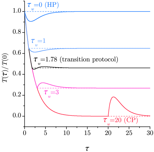
Figure 1: Illustration of the protocols considered in this work. The granular gas is prepared in an initial state ($\tau=0$) for which all the energy is concentrated in the translational degrees of freedom, as described in the text. In a first stage, $0<\tau<\tau_{w}$, the granular gas freely cools. Then, at the waiting time $\tau=\tau_{w}$, the noise intensity is suddenly increased from zero to a value such that the instantaneous temperature $T(\tau_{w})$ coincides with the corresponding steady temperature $T_{\mathrm{st}}$. The curves shown for $\tau>\tau_{w}$ correspond to the so-called normal Kovacs response. Time $\tau$ measures the average number of collisions per particle. Note that, in order to visualize the Kovacs effect, the relative deviations of $T(\tau)$ from $T_{\mathrm{st}}$ in the response curves have been magnified by a factor $r=5$ for all the protocols, except for the transition one, for which $r=100$. All the curves correspond to normal and tangential restitution coefficients $\alpha=0.8$ and $\beta=0$, respectively.

3 Results and Discussion

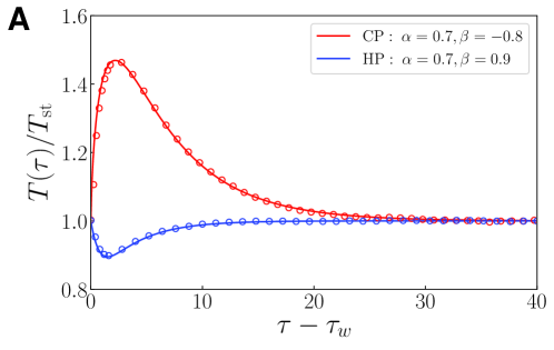
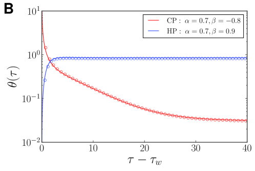
Figure 2: Large Kovacs humps in the granular gas. Panel A shows two examples of macroscopic Kovacs humps for a granular gas with $\alpha=0.7$. The upper curve corresponds to the CP (with $\beta=0.9$) whereas the lower curve corresponds to the HP (with $\beta=-0.8$), as measured in MD simulations. Panel B shows the time evolution of the corresponding rotational-to-translational temperature ratio $\theta=T_{r}/T_{t}$. The simulation results show an almost perfect agreement with our theoretical predictions (lines).

Two data sets from molecular dynamics (MD) simulations (see B) of the granular gas for both the HP and the CP, together with their corresponding theoretical predictions, are represented in Fig. 2A, which clearly shows the appearance of very large memory effects. The temperature humps displayed here, of approximately $100\%$ for the CP and $10\%$ for the HP, are larger by at least two orders of magnitude than previously observed memory effects in athermal systems, which at most range from a few thousandths to a few hundredths of the stationary value of the relevant variable [17, 19]. The theoretical curves displayed in Fig. 2A have been obtained by means of a bi-variate Maxwellian approximation, in which all the cumulants are assumed to be zero (see A). Thus, the essential property driving the giant memory effect here is the existence of two independent temperature scales, translational and rotational, i.e., the breakdown of equipartition as given by the fact that $\theta\neq 1$. This is further illustrated in Fig. 2B, which shows $\theta(\tau)$ for the same cases as in Fig. 2A. Again, the agreement between theory and simulation is excellent, even at the level of the two contributions to the total temperature. Note that the relaxation time in the CP case is much longer than in the HP one.

Let us denote the earliest minimum and maximum in the temperature evolution as $T_{m}$ and $T_{M}$, respectively. We also define $\mathcal{H}_{m}\equiv T_{m}/T_{\mathrm{st}}-1<0$, $\mathcal{H}_{M}\equiv T_{M}/T_{\mathrm{st}}-1>0$, accordingly. In Fig. 3 we present contour plots highlighting the regions with large $|\mathcal{H}_{m}|$ (HP normal response, CP anomalous response) and $\mathcal{H}_{M}$ (HP anomalous response, CP normal response). We also plot the transition line $\mathcal{H}_{M}=|\mathcal{H}_{m}|$ from normal to anomalous response. Huge Kovacs humps appear, especially in the normal region for the CP, in which the size of reported humps can be as large as $100\%$, relative to the steady temperature.

In order to characterize and quantify complexity in the thermal response we define the parameter $\mathcal{S}$,

$$\mathcal{S}=\mathrm{sgn}({\mathcal{H}_{1}})\frac{\min(|\mathcal{H}_{m}|,\mathcal{H}_{M})}{\max(|\mathcal{H}_{m}|,\mathcal{H}_{M})},$$ (4)

where $\mathcal{H}_{1}$ (equal to either $\mathcal{H}_{m}$ or $\mathcal{H}_{M}$) is the magnitude of the earliest extremum. Note that $\mathcal{S}=0$ if there is only one extremum. Thus, $\mathcal{S}\neq 0$ is the signature of the emergence of more complex response, i.e., with more than one extremum, in the normal-to-anomalous transition. In the transition region, $|\mathcal{S}|$ attains its maximum value, $|\mathcal{S}|=1$, when both extrema are of the same size and neither dominates. The sign of $\mathcal{S}\in[-1,1]$ is equal to that of the earliest extremum, providing further information on the detailed structure of the response.

Figure 4 represents $\mathcal{S}$ as a function of the coefficients of restitution $\alpha,\beta$, by solving the system of Eqs. (1) and (2). Panels A, C, and D correspond to the HP, whereas panels B and E correspond to the CP. We have highlighted in blue (red) regions with $\mathcal{S}<0$ ($\mathcal{S}>0$), whereas all points with “simple” memory behavior, i.e., $\mathcal{S}=0$, remain white. The complex regions are thin but still occupy noticeable sections of the parameter space, especially taking into account that they fall into ranges of experimental values of $\alpha$ and $\beta$ commonly present in a variety of materials [23]. In Fig. 4A (HP), we clearly observe two zones rich in complex memory effects. In panel C, the first complex zone is zoomed in. This region is attached to the smooth limit, $\beta\sim-1$, and only displays $\mathcal{S}>0$ for high inelasticities, up to $\alpha=1/\sqrt{2}$. In panel D, the second complex region is zoomed in. Within this region, which is close to the quasielastic limit $\alpha\sim 1$, the system displays both $\mathcal{S}>0$ and $\mathcal{S}<0$ behavior. In Fig. 4B (CP), only one complex Kovacs region next to the quasielastic limit, inside which $\mathcal{S}>0$, has been identified. Panel E shows a close-up thereof.

It is important to mention that we have found that all the details of the complex regions emerge in the theoretical solution only when the cumulants are taken into account. This indicates that the temperatures $T_{t}$ and $T_{r}$ do not explain in full detail by themselves the complexity of memory effects found in the rough granular gas. Let us also point out that we have found for the HP a critical narrow region with a discontinuous transition from $\mathcal{S}>0$ to $\mathcal{S}<0$, which is signaled in panel D in Fig. 4 and represented in time evolution curves in Fig. 5.

In this critical region, the system displays several different mechanisms for the transition from complex to simple—only one extremum—behavior. The latter can be either the normal behavior of molecular systems [1, 9, 15] (also present in nonequilibrium systems) or the anomalous behavior exclusive of nonequilibrium systems [17, 19]. This is appropriately tagged in panels A and B of Fig. 4, in which we have labeled the corresponding normal and anomalous regions. In the narrow critical region, $\mathcal{S}$ discontinuously jumps from (small) negative to positive values and three consecutive temperature extrema appear before stabilization in the stationary value is attained. Otherwise, $\mathcal{S}$ has a well-defined sign and the transition from complex to simple is continuous.

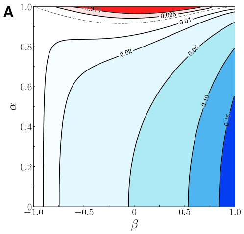
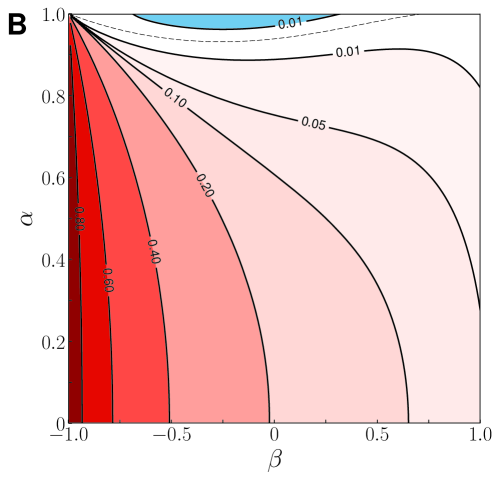
Figure 3: Contour plots of large extrema in the Kovacs response. Large minima ($|\mathcal{H}_{m}|$) are represented by bluish contours and large maxima ($\mathcal{H}_{M}$) by reddish contours. Dashed lines indicate the $\mathcal{H}_{M}=|\mathcal{H}_{m}|$ transition curves, for which the predominant extremum changes sign, from maximum to minimum and vice versa. Above and below these curves we find $\mathcal{H}_{M}>|\mathcal{H}_{m}|$ ($\mathcal{H}_{M}<|\mathcal{H}_{m}|$) and $\mathcal{H}_{M}<\mathcal{H}_{m}$ ($\mathcal{H}_{M}>|\mathcal{H}_{m}|$) behaviors, respectively, in the HP (CP). (A) Heating protocol (HP). (B) Cooling protocol (CP).

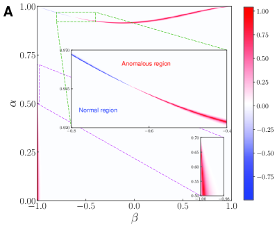
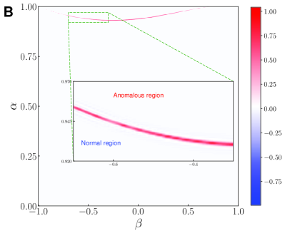
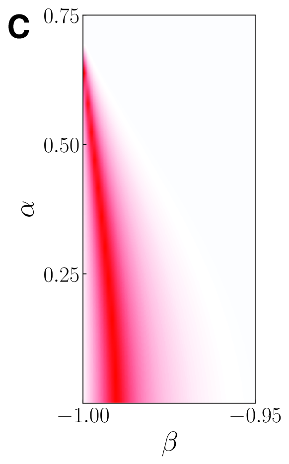
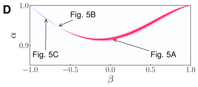
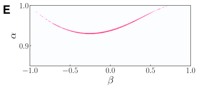
Figure 4: Kovacs complexity ($\mathcal{S}$) phase diagrams. Density plot of $\mathcal{S}$ vs. the $\alpha,\beta$ complete space parameter: (A) for the HP; (B) for the CP. (C, D) Insets of complex memory regions next to the smooth and the quasielastic limits, respectively, for the HP. (E) Inset of the complex memory region next to the quasielastic limit for the CP. In the HP, as seen in panels A and D, three different types of transition exist: $\mathcal{S}<0$ (bluish, $\beta<-0.65$), $\mathcal{S}>0$ (reddish, $\beta>-0.65$), and the intermediate mechanism ($\mathcal{S}\approx 0$) for $\beta\approx-0.65$, as depicted below in Fig. 5B. However, in the CP, see panels B and E, only a $\mathcal{S}>0$-type transition has been observed.

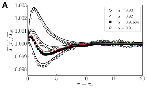
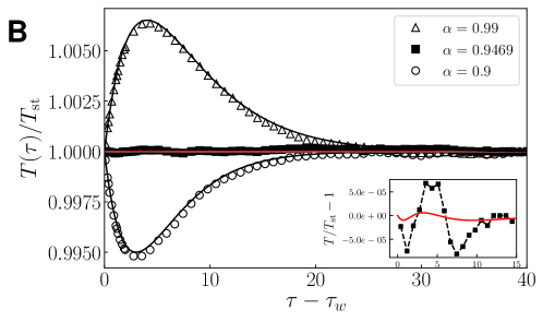
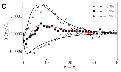
Figure 5: Mechanisms for the transition from normal to anomalous in the HP. There are three of these mechanisms, which are shown here by DSMC simulations (symbols) and our theoretical approach (lines). Specifically, through (A) $\mathcal{S}>0$ at $\beta=0$, (B) $\mathcal{S}\approx 0$ (actually a triple Kovacs hump transition mechanism; see inset, where the line joining the simulation points is a guide to the eye) at $\beta=-0.65$, and (C) $\mathcal{S}<0$ at $\beta=-0.8$. In order to assist in locating these transitions in the parameter plane $(\alpha,\beta)$, their positions have been annotated in Fig. 4D.

Figure 5 displays the evolution curves of the temperature for the three different Kovacs transitions that we have found, in all cases depicted here for the HP: the $\mathcal{S}>0$ transition in panel A, the $\mathcal{S}\approx 0$ transition in panel B (in its inset we show the three consecutive humps), and finally the $\mathcal{S}<0$ case in panel C. All theoretical curves are compared against the numerical solution of the kinetic equation, obtained by means of the direct simulation Monte Carlo (DSMC) method (see B). The agreement is in general excellent, which once more shows the accuracy of our theoretical approach. Although the size of the humps in the transition regions appear smaller than those in Fig. 2A with simple memory behavior, yet they are of the same order of magnitude as those previously reported in the smooth granular gas [17].

4 Conclusions

Our work puts forward a general mechanism for the emergence of significantly large memory effects. Enormous humps can be expected if the time evolution of the system under scrutiny is controlled by at least two independent and comparable in magnitude physical variables (here the translational and rotational temperatures) but with only one (here the total temperature) being relevant for the macroscopic or hydrodynamic description. In addition, complex Kovacs response, with more than one extremum, can be expected if the time evolution of the system depends on several additional relevant variables. Here, these additional variables are the fourth-order cumulants, whose sometimes nonmonotonic relaxation [25] probably enhances memory effect complexity.

So far, and despite the large number of previous works on analogous phenomena, only one extremum in the Kovacs response has been reported. In thermal systems, in which the usual fluctuation-dissipation theorem holds and the stationary (equilibrium) distribution has the canonical shape, this is consistent with linear response results that predict normal behavior with only one maximum [16]. In athermal systems, the Kovacs response also includes anomalous behavior, but once more only one extremum has been observed [17, 19]. Therefore, an interesting prospect is elucidating whether or not the nonlinear theoretical framework developed in Ref. [19] allows for complex response with more than one extremum.

Memory effects of the size and complexity we have observed here can potentially be present in other athermal or molecular systems. Several variables of comparable magnitude must be coupled in their time evolution in nonlinear form, even if only a subset thereof is relevant in the macroscopic description. This may be relevant, for instance, in active matter systems, where nonlinear effects are important in general [19, 29]. We think our results are also especially significant for future experimental work, since we expect these large memory effects to be measurable in granular dynamics experiments; a thermally homogeneous system may be achieved by means of homogeneous turbulent air fluidization [28].

Acknowledgements

The authors thank Prof. J. S. Urbach for fruitful discussions. This work has been supported by the Spanish Agencia Estatal de Investigación Grants (partially financed by the ERDF) No. MTM2017-84446-C2-2-R,  MTM2014-56948-C2-2-P (A.L.), and No. FIS2016-76359-P (F.V.R. and A.S.), and also by Universidad de Sevilla’s VI Plan Propio de Investigación Grant PP2018/494 (A.P.). Use of computing facilities from Extremadura Research Centre for Advanced Technologies (CETA-CIEMAT), funded by the ERDF is also acknowledged.

Appendix A Theory

The stochastic force ($\mathbf{F}^{\mathrm{wn}}$) has the form of a white noise: $\langle{\bf F}_{i}^{\mathrm{wn}}(t)\rangle={\bf 0}$, $\langle{\bf F}_{i}^{\mathrm{wn}}(t){\bf F}_{j}^{\mathrm{wn}}(t^{\prime})\rangle=\mathsf{I}\,m^{2}\chi_{0}^{2}\delta_{ij}\delta(t-t^{\prime})$, where indexes $i,j$ refer to particles, $\mathsf{I}$ is the $3\times 3$ unit matrix, and $\chi_{0}^{2}$ is the white noise intensity. In homogeneous states, the Boltzmann–Fokker–Planck equation characterizing the evolution of a granular gas submitted to the stochastic external force $\mathbf{F}^{\mathrm{wn}}$ is written as [25]

$$\left(\partial_{t}-\frac{\chi_{0}^{2}}{2}\nabla_{\mathbf{v}}^{2}\right)f(\mathbf{v},\boldsymbol{\omega};t)={J[\mathbf{v},\boldsymbol{\omega}|f(t)]}.$$ (5)

Above, $f(\mathbf{v},\boldsymbol{\omega};t)$ is the velocity distribution function ($\mathbf{v}$ and $\boldsymbol{\omega}$ being the translational and angular velocities, respectively) and $J[\mathbf{v},\boldsymbol{\omega}|f]$ is the collision integral in the (inelastic) Boltzmann equation for rough spheres, which accounts for the collision rules [25]

$$\widehat{\boldsymbol{\sigma}}\cdot\mathbf{u}^{\prime}=-\alpha\,\widehat{{\boldsymbol{\sigma}}}\cdot\mathbf{u},\quad\widehat{{\boldsymbol{\sigma}}}\times\mathbf{u}^{\prime}=-\beta\,\widehat{{\boldsymbol{\sigma}}}\times\mathbf{u}.$$ (6)

Here, the primes denote postcollisional values, $\widehat{{\boldsymbol{\sigma}}}$ is the unit collision vector joining the centers of the two colliding spheres (from the center of particle 1 to the center of particle 2) and $\mathbf{u}=\mathbf{v}_{1}-\mathbf{v}_{2}-{\frac{\sigma}{2}}\widehat{{\boldsymbol{\sigma}}}\times({\boldsymbol{\omega}}_{1}+{\boldsymbol{\omega}}_{2})$ is the relative velocity of the spheres at their contact point. The coefficient of normal restitution $\alpha$ takes values between $0$ (completely inelastic collision) and $1$ (completely elastic collision), while the coefficient of tangential restitution $\beta$ takes values between $-1$ (completely smooth collision, unchanged angular velocities) and $1$ (completely rough collision) [24].

Given any one-particle function $A(\mathbf{v},\boldsymbol{\omega})$, its average is defined as $\langle A(t)\rangle=n^{-1}\int d\mathbf{v}\int d\boldsymbol{\omega}\,A(\mathbf{v},\boldsymbol{\omega})f(\mathbf{v},\boldsymbol{\omega};t)$, where the number density is given by $n=\int d\mathbf{v}\int d\boldsymbol{\omega}\,f(\mathbf{v},\boldsymbol{\omega};t)$. The basic physical properties are the translational ($T_{t}$), rotational ($T_{r}$), and total ($T$) granular temperatures, i.e.,

$${T_{t}={\frac{m}{3}}\langle v^{2}\rangle,\quad T_{r}={\frac{I}{3}}\langle\omega^{2}\rangle,}\quad{T=\frac{T_{t}+T_{r}}{2}=T_{t}\frac{1+\theta}{2}},$$ (7)

where $I$ is the moment of inertia. We have introduced the temperature ratio $\theta\equiv T_{r}/T_{t}$, which is relevant for the analysis that follows and whose steady-state value is independent of the driving amplitude $\chi_{0}^{2}$. The evolution equations for $T_{t}$, $T_{r}$, and $T$ are

$$\partial_{t}T_{t}-{m\chi_{0}^{2}}=-\xi_{t}T_{t},\quad{\partial_{t}T_{r}=-\xi_{r}T_{r}},$$ (8)

$$\partial_{t}T-\frac{m\chi_{0}^{2}}{2}=-\zeta T.$$ (9)

The equations for $T_{t}$ and $T_{r}$ have been obtained by multiplying both sides of Eq. (5) by the translational and rotational kinetic energies, respectively, and integrating over all particle velocity values. The parameters $\xi_{t}$ and $\xi_{r}$ are

$$\xi_{t}=-{\frac{m}{3nT_{t}}}\int d\mathbf{v}\int d{\boldsymbol{\omega}}\,v^{2}{J[\mathbf{v},{\boldsymbol{\omega}}|f]},$$ (10)

$$\xi_{r}=-{\frac{I}{3nT_{r}}}\int d\mathbf{v}\int d{\boldsymbol{\omega}}\,\omega^{2}{J[\mathbf{v},{\boldsymbol{\omega}}|f]},$$ (11)

respectively. In general, neither $\xi_{t}$ nor $\xi_{r}$ does have a definite sign, whereas the cooling rate,

$$\zeta=\frac{\xi_{t}T_{t}+\xi_{r}T_{r}}{2T}=\frac{\xi_{t}+\xi_{r}{\theta}}{1+\theta},$$ (12)

is always positive because energy is dissipated in collisions.

To proceed further, it is convenient to go to dimensionless variables. Time is measured in a scale $\tau$,

$$\tau=\frac{1}{2}\int_{0}^{t}dt^{\prime}\,\nu(t^{\prime}),\quad\nu(t)=4n\sigma^{2}\sqrt{\pi T_{t}(t)/m},$$ (13)

which is roughly the accumulated number of collisions per particle, because $\nu(t)$ is the collision frequency. Dimensionless velocities are introduced as

$$\mathbf{c}(t)\equiv\frac{\mathbf{v}}{\sqrt{2T_{t}(t)/m}},\quad\mathbf{w}(t)\equiv\frac{{\boldsymbol{\omega}}}{\sqrt{2T_{r}(t)/I}},$$ (14)

a reduced velocity distribution function as

$$\phi(\mathbf{c},\mathbf{w};\tau)\equiv\frac{1}{n}\left[\frac{4T_{t}(t)T_{r}(t)}{mI}\right]^{3/2}f(\mathbf{v},{\boldsymbol{\omega}};t),$$ (15)

and the dimensionless collision kernel as

$$\mathcal{J}[\mathbf{c},\mathbf{w}|\phi(\tau)]=\frac{2}{n\nu(t)}\left[\frac{4T_{t}(t)T_{r}(t)}{mI}\right]^{3/2}J[\mathbf{v},{\boldsymbol{\omega}}|f(t)].$$ (16)

In dimensionless variables, the evolution equations for the temperatures can be written as Eqs. (1) and (2) in the main text. Therein, there appear the reduced collisional moments $\mu_{20}\equiv\mu_{20}^{(0)}$ and $\mu_{02}\equiv\mu_{02}^{(0)}$, where

$$\mu_{pq}^{(r)}(\tau)\equiv-\int d\mathbf{c}\int d\mathbf{w}\,c^{p}w^{q}(\mathbf{c}\cdot\mathbf{w})^{r}{\mathcal{J}[\mathbf{c},\mathbf{w}|\phi(\tau)]}.$$ (17)

Note that, aside from the nondimensionalizing factors, the production rates $\xi_{t}$ and $\xi_{r}$ are basically identical to $\mu_{20}$ and $\mu_{02}$, respectively. These are functionals of the whole distribution function and thus the evolution equations for the temperatures are not closed.

In order to close the dynamical equations, a formally exact expansion in orthogonal polynomials can be performed [25]. For isotropic states, we can expand the velocity distribution around the Maxwellian $\phi_{M}(c,w)=\pi^{-3}e^{-c^{2}-w^{2}}$,

$$\phi(\mathbf{c},\mathbf{w};\tau)=\phi_{M}(c,w)\sum_{j=0}^{\infty}\sum_{k=0}^{\infty}\sum_{\ell=0}^{\infty}a_{jk}^{(\ell)}(\tau)\Psi_{jk}^{(\ell)}(\mathbf{c},\mathbf{w}),$$ (18)

where $\Psi_{jk}^{(\ell)}(\mathbf{c},\mathbf{w})$ are certain products of Laguerre and Legendre polynomials. By normalization, $a_{00}^{(0)}=1$, $a_{10}^{(0)}=a_{01}^{(0)}=0$, and the lowest nontrivial coefficients are those associated with moments of degree four, namely

$$a_{20}^{(0)}=\frac{4}{15}\langle c^{4}\rangle-1,\quad a_{02}^{(0)}=\frac{4}{15}\langle w^{4}\rangle-1,$$ (19)

$$a_{11}^{(0)}=\frac{4}{9}\langle c^{2}w^{2}\rangle-1,\quad a_{00}^{(1)}=\frac{8}{15}\left[\langle(\mathbf{c}\cdot\mathbf{w})^{2}\rangle-\frac{1}{3}\langle c^{2}w^{2}\rangle\right],$$ (20)

which we call the fourth-order cumulants henceforth.

Maxwellian approximation.- The simplest description is obtained by substituting the Maxwellian velocity distribution into the collision integrals (17). Equivalently, one may consider that all the nontrivial cumulant vanish in this approach, which yields

$$\mu_{20,M} =1-\alpha^{2}+\frac{\kappa(1+\beta)}{(1+\kappa)^{2}}\left[2+\kappa(1-\beta)-\theta(1+\beta)\right],$$ (21)

$$\mu_{02,M} =\frac{\kappa(1+\beta)}{(1+\kappa)^{2}}\left[2+\kappa^{-1}(1-\beta)-\theta^{-1}(1+\beta)\right].$$ (22)

where $\kappa\equiv 4I/m\sigma^{2}$ is the dimensionless moment of inertia. Insertion of Eq. (21) into the evolution equations (1) and (2) in the main text gives rise to the Maxwellian approximation.

First Sonine approximation.- A more elaborate approximation can be done by incorporating the lowest order cumulants, which we defined in Eqs. (19) and (20), as the first corrections to the Maxwellian.

A closed set of six coupled differential equations can be obtained for $\theta(\tau)$, $\gamma(\tau)$, $a_{20}^{(0)}(\tau)$, $a_{02}^{(0)}(\tau)$, $a_{11}^{(0)}(\tau)$, and $a_{00}^{(1)}(\tau)$. To do so, explicit—yet not exact—expressions for the collision integrals $\mu_{pq}^{(r)}$ with $p+q+2r=2$ and $4$ are derived in terms of $\theta$ and those lowest order cumulants. These rather involved expressions can be found in the Supplemental Material of Ref. [25], and are thus omitted here. The resulting set of six differential equations can be numerically solved with appropriate initial conditions for each physical situation, as discussed in the main text. In this way, we obtain the time evolution of the temperatures in the so-called first Sonine approximation, to which we refer throughout this work.

Appendix B Computer simulations

We use in this work data sets obtained from computer simulations from two independent and different methods: direct simulation Monte Carlo (DSMC) method, which obtains an exact numerical solution of the relevant kinetic equation [in our case Eq. (5)] and molecular dynamics (MD) simulation, which solves particles trajectories. A detailed description of the DSMC method may be found elsewhere [30]. In our DSMC simulations, and in order to reduce statistical noise in the temperature time evolution curves, we have used an average of 100 statistical replicas of a system with $2\times 10^{6}$ particles. In the MD case, we have simulated 1000 inelastic hard spheres at a density $n\sigma^{3}=0.01$ and averaged over 500 trajectories.

References

- [1] A. J. Kovacs, J. J. Aklonis, J. M. Hutchinson, and A. R. Ramos. Isobaric volume and enthalpy recovery of glasses. II. A transparent multiparameter theory. J. Polym. Sci. Pt. B-Polym. Phys., 17:1097–1162, 1979.
- [2] G. F. Rodriguez, G. G. Kenning, and R. Orbach. Full aging in spin glasses. Phys. Rev. Lett., 91:3, 2003.
- [3] P. Meyer, S. Léonard, L. Berthier, J. P. Garrahan, and P. Sollich. Activated aging dynamics and negative fluctuations-dissipation ratios. Phys. Rev. Lett., 96:030602, 2006.
- [4] T. Xie. Tunable polymer multi-shape memory effect. Nature, 416:267–270, 2010.
- [5] D. Fiocco, G. Foffi, and S. Sastry. Encoding of memory in sheared amorphous solids. Phys. Rev. Lett., 112:025702, 2014.
- [6] R. Hecht, S. F. Cieszymski, E. V. Colla, and M. B. Weissman. Aging dynamics in ferroelectric deuterated potassium dihydrogen phosphate. Phys. Rev. Materials, 1:044403, 2017.
- [7] S. S. Schoenholz, E. D. Cubuk, E. Kaxiras, and A. J. Liu. Relationship between local structure and relaxation in out-of-equilibrium glassy systems. Proc. Natl. Acad. Sci. U. S. A., 114:263–267, 2017.
- [8] S. R. Nagel. Experimental soft-matter science. Rev. Mod. Phys., 89:025002, 2017.
- [9] L. Berthier and J. P. Bouchaud. Geometrical aspects of aging and rejuvenation in the ising spin glass: A numerical study. Phys. Rev. B, 66:054404, 2002.
- [10] L. M. C. Janssen, A. Kaiser, and H. Löwen. Aging and rejuvenation of active matter under topological constraints. Sci. Rep., 7:5667, 2017.
- [11] C. L. Struik. Physical Aging in Amorphous Polymers and Other Materials. Elsevier, Amsterdam, UK, 1980.
- [12] E. B. Mpemba and D. G. Osborne. Cool? Phys. Educ., 4:172–175, 1969.
- [13] A. Lasanta, F. Vega Reyes, A. Prados, and A. Santos. When the hotter cools more quickly: Mpemba effect in granular fluids. Phys. Rev. Lett., 119:148001, 2017.
- [14] M. Baity-Jesi, E. Calore, A. Cruz, L.A. Fernandez, J.M. Gil-Narvion, A. Gordillo-Guerrero, D. Iñiguez, A. Lasanta, A. Maiorano, E. Marinari, V. Martin-Mayor, J. Moreno-Gordo, A. Muñoz-Sudupe, D. Navarro, G. Parisi, S. Perez-Gaviro, F. Ricci-Tersenghi, J.J. Ruiz-Lorenzo, S.F. Schifano, B. Seoane, A. Tarancon, R. Tripiccione, and D. Yllanes. Mpemba effect in spin glasses: A persistent memory effect. Proc. Natl Acad. Sci. USA, in press, 2019.
- [15] S. Mossa and F. Sciortino. Crossover (or Kovacs) effect in an aging molecular liquid. Phys. Rev. Lett., 92:045504, 2004.
- [16] A. Prados and J. J. Brey. The Kovacs effect: a master equation analysis. J. Stat. Mech., P02009, 2010.
- [17] A. Prados and E. Trizac. Kovacs-Like Memory Effect in Driven Granular Gases. Phys. Rev. Lett., 112:198001, 2014.
- [18] C. A. Plata and A. Prados. Kovacs-Like Memory Effect in Athermal Systems: Linear Response Analysis. Entropy, 19:539, October 2017.
- [19] R. Kürsten, V. Sushkov, and T. Ihle. Giant Kovacs-like memory effect for active particles. Phys. Rev. Lett., 119:188001, 2017.
- [20] Y. Lahini, O. Gottesman, A. Amir, and S. M. Rubinstein. Nonmonotonic Aging and Memory Retention in Disordered Mechanical Systems. Phys. Rev. Lett., 118:085501, February 2017.
- [21] P. K. Haff. Grain flow as a fluid-mechanical phenomenon. J. Fluid Mech., 134:401–430, 1983.
- [22] I. S. Aranson and L. S. Tsimring. Patterns and collective behavior in granular media: Theoretical concepts. Rev. Mod. Phys, 78:641–692, 2006.
- [23] S. F. Foerster, M. Y. Louge, H. Chang, and K. Allis. Measurements of the collision properties of small spheres. Phys. Fluids, 6:1108–1115, 1994.
- [24] S. G. Brush. Kinetic theory, volume 3 of International Series of Monographs in Natural Philosophy 42. Pergamon Press, Oxford, UK, 1972.
- [25] F. Vega Reyes, A. Santos, and G. M. Kremer. Role of roughness on the hydrodynamic homogeneous base state of inelastic spheres. Phys. Rev. E, 89:020202(R), 2014.
- [26] F. Vega Reyes and A. Santos. Steady state in a gas of inelastic rough spheres heated by a uniform stochastic force. Phys. Fluids, 27:113301, 2015.
- [27] D. R. M. Williams and F. C. MacKintosh. Driven granular media in one dimension: correlations and equation of state. Phys. Rev. E, 54:R9–R12, 1996.
- [28] R. P. Ojha, P.-A. Lemieux, P. K. Dixon, A. J. Liu, and D. J. Durian. Statistical mechanics of a gas-fluidized particle. Nature, 427:521–523, 2005.
- [29] M. C. Marchetti, J. F. Joanny, S. Ramaswamy, T. B. Liverpool, J. Prost, M. Rao, and R. Aditi Simha. Hydrodynamics of soft active matter. Rev. Mod. Phys., 85:1143–1189, 2013.
- [30] G. A. Bird. Molecular Gas Dynamics and the Direct Simulation of Gas Flows. Clarendon, Oxford, UK, 1994.