Truth Inference on Sparse Crowdsourcing Data with Local Differential Privacy

Abstract

Crowdsourcing has arisen as a new problem-solving paradigm for tasks that are difficult for computers but easy for humans. However, since the answers collected from the recruited participants (workers) may contain sensitive information, crowdsourcing raises serious privacy concerns. In this paper, we investigate the problem of protecting answer privacy under local differential privacy (LDP), by which individual workers randomize their answers independently and send the perturbed answers to the task requester. The utility goal is to enable to infer the true answer (i.e., truth) from the perturbed data with high accuracy. One of the challenges of LDP perturbation is the sparsity of worker answers (i.e., each worker only answers a small number of tasks). Simple extension of the existing approaches (e.g., Laplace perturbation and randomized response) may incur large error of truth inference on sparse data. Thus we design an efficient new matrix factorization (MF) algorithm under LDP. We prove that our MF algorithm can provide both LDP guarantee and small error of truth inference, regardless of the sparsity of worker answers. We perform extensive experiments on real-world and synthetic datasets, and demonstrate that the MF algorithm performs better than the existing LDP algorithms on sparse crowdsourcing data.

I Introduction

Crowdsourcing enables to perform tasks that are easy for humans but remain difficult for computers. Typically, a task requester releases the tasks on a crowdsourcing platform (e.g., Amazon Mechanical Turk (AMT)). Then the workers provide their answers to these tasks on the same crowdsourcing platform in exchange for a reward. As the Internet and mobile technologies continue to advance, crowdsourcing helps organizations to improve productivity and innovation in a cost-effective way.

While crowdsourcing provides an effective way for problem-solving, collecting individual worker answers may pose potential privacy risks on the workers. For instance, it has been reported that AMT was leveraged by politicians to access a large pool of Facebook profiles and collect tens of thousands of individuals’ demographic data [2]. Crowdsourcing-related applications such as participatory sensing [8] and citizen science [7] also raise privacy concerns for the workers. However, simply removing the worker names or replacing the names with pseudo-names cannot adequately protect worker privacy. It is still possible to de-anonymize crowd workers by matching their inputs with external datasets [27].

Recently, differential privacy (DP) [17] has been used in many applications to provide rigorous privacy guarantee. Classical DP requires a centralized trusted data curator (DC) to collect all the answers and publish privatized statistical information. However, as crowdsourcing services become increasingly popular, many untrusted task requesters (or DCs) appear to abuse the crowdsourcing services by collecting private information of the workers (see the aforementioned example that AMT was leveraged by politicians). In recent years, local differential privacy (LDP) [15] arises as a good alternative paradigm to prevent an untrusted DC from learning any personal information of the data providers and provides per-user privacy. In LDP, each data provider randomizes his/her data to satisfy DP locally. Then the data providers send their randomized answers to the (untrusted) DC, who aggregates the data with no access to personal information of data providers. LDP roots in randomized response, first proposed in [48]. It has been used in many applications such as Google’s Chrome browser [19, 20] and Apple’s iOS 10 [1].

The goal of this paper is to protect worker privacy with LDP guarantee for crowdsourcing systems. We aim to address two main challenges.

Challenge 1: sparsity of worker answers. The worker answers can be very sparse, as often times most workers only provide answers to a very small portion of the tasks. For example, the analysis of a real-world crowdsourcing dataset, named AdultContent dataset, which includes the relevance ratings of 825 workers for approximately 11,000 documents, shows that the dataset has the average sparsity as high as 99% (i.e., each worker rates 70 documents at average). The NULL values in worker answers (i.e., missing answers from the workers) should be protected, as they reveal the sensitive information as whether a worker has participated in specific tasks [13]. However, careless perturbation of NULL values may alter the original answer distribution and incur significant inaccuracy of truth inference. However, most of the LDP works (e.g., [5, 4, 37, 46]) only consider complete data. None of these works address the sparsity issue.

Challenge 2: data utility. One of the major utility goals of crowdsourcing systems is to aggregate the answers from workers of different (possibly unknown) quality, and infer the true answer (i.e., truth) of each task. Truth inference [32, 51] has been shown as effective to estimate both worker quality and the truth. Most of the existing truth inference mechanisms follow an iterative process: both worker quality and inferred truth are estimated and updated iteratively, until they reach convergence. This makes it extremely difficult to preserve the accuracy of truth inference on the perturbed worker answers, as even the slight amount of initial noise on the worker answers may be propagated during iterations and amplified to the final truth inference results.

Matrix factorization is one of the most popular methods to predict NULL values. Intuitively, by matrix factorization, the answers of a specific worker can be modeled as the multiplication of a worker profile vector and a task profile matrix. We observe that the adaption of a worker profile vector only relies on the worker’s own answers rather than those of other workers. Therefore, matrix factorization can be performed locally. However, applying LDP to matrix factorization is not trivial. A direct application of LDP on the worker answers can incur a large perturbation error that linearly grows with the number of tasks. Most of the existing methods of matrix factorization with LDP [24, 40, 41, 42] only consider recommender systems. They cannot be applied to the crowdsourcing setting directly due to the mismatched utility function; they consider the accuracy of recommendation while we consider the accuracy of truth inference. Furthermore, some of these works (e.g., [24, 42]) require iterative feedbacks between the data curator and users, which may incur expensive communication overhead.

Contributions. To our best knowledge, this is the first work that provides privacy protection on sparse worker answers with LDP guarantee, while preserving the accuracy of truth inference on the perturbed data. We summarize our main contributions as follows. First, we present simple extension of two existing perturbation approaches, namely Laplace perturbation (LP) and randomized response (RR), to deal with sparse crowdsourcing data. We provide detailed analysis of the expected error bound of truth inference for these two approaches, and show that both LP and RR can have large error of truth inference for sparse data. Second, we design a new matrix factorization (MF) algorithm with LDP. To preserve the accuracy of truth inference, we apply the perturbation on the objective function of matrix factorization, instead of on the matrix factorization results. Our formal analysis shows that the theoretical error bound of truth inference results on the perturbed data is small, and the error bound of truth inference is insensitive to data sparsity. Finally, we conduct extensive experiments on real-world and synthetic crowdsourcing datasets of various sparsity. The experimental results demonstrate that our MF approach significantly improves the accuracy of truth inference on the perturbed data compared with the existing work.

The rest of this paper is organized as follows. Section II and III present the background and preliminaries. Section IV introduces the extension of two existing approaches. Section V discusses our MF mechanism. Section VI presents the experiment results. Related work is discussed in Section VII. Section VIII concludes the paper.

II Background

In this section, we briefly recall the definition of local differential privacy, and overview the truth inference algorithms. The notations used in the paper are shown in Table I.

Symbol	Meaning
$m$	# of workers
$n$	# of tasks
$\vec{a}_{i}$	Worker $W_{i}$’s original answer vector
$\hat{a}_{j}$	Worker $W_{i}$’s answer vector after perturbation
$a_{i,j}$	Worker $W_{i}$’s answer to task $T_{j}$
$\Gamma$	Domain of task answers (excluding NULL answers)
$\sigma_{i}$	Standard deviation of worker $W_{i}$’s answer error
$q_{i}$	Estimated quality of worker $W_{i}$
$\mu_{j}$/$\hat{\mu_{j}}$	Real/estimated truth of task $T_{j}$
$s_{i}$	Percentage of tasks that $W_{i}$ returns non-NULL values
$\epsilon$	Privacy budget
$\mathcal{T}_{i}$	The set of tasks that worker $W_{i}$ performs
$d$	Factorization parameter

TABLE I: Notations

II-A Local Differential Privacy (LDP)

The need for data privacy arises in two different contexts: the local privacy context in which the individuals disclose their personal information (e.g., participation in surveys for specific population), and the global privacy context in which the institutions release aggregation information of their data (e.g., US Government releases census data). The classic concept of differential privacy (DP) [17] is proposed in the global privacy context. In a nutshell, DP ensures that an adversary cannot infer whether or not a particular individual is participating in the database query, even with unbounded computational power and access to every entry in the database except for that particular individual’s data. DP considers a centralized setting that includes a trusted data curator, who generates the perturbed statistical information (e.g., counts and histograms) by using a randomized mechanism [23, 31, 35, 49]. Recently, a variant of DP, named local differential privacy (LDP) [29, 15] was proposed for the decentralized setting where multiple data providers send their private data to a untrusted data curator. Before sending it to the data curator, each data provider perturbs his private data locally by using a differentially private mechanism. The randomized response method [48] has been used to provide local privacy when individuals respond to sensitive surveys. Intuitively, for a given survey question, respondents provide a truthful answer with probability $p>1/2$ and lie with probability $1-p$. The randomized response method provides $(ln\frac{p}{1-p})$-LDP [46].

While LDP considers per-user privacy, in this paper, we consider per-user per-answer privacy. Therefore, by following [38], we define a variant of LDP [15], named $\epsilon$-cell local differential privacy, below.

Definition II.1 ($\epsilon$-cell Local Differential Privacy).

A randomized privatization mechanism $\mathcal{M}$ satisfies $\epsilon$-cell local differential privacy ($\epsilon$-cell LDP) iff for any pair of answer vectors $\vec{a}$ and $\vec{a}^{\prime}$ that differ at one cell, we have:

$$\forall\vec{z}_{p}\in Range(\mathcal{M}):\frac{Pr[\mathcal{M}(\vec{a})=\vec{z}_{p}]}{Pr[\mathcal{M}(\vec{a}^{\prime})=\vec{z}_{p}]}\leq e^{\epsilon},$$

where $Range(\mathcal{M})$ denotes the set of all possible outputs of the algorithm $\mathcal{M}$.

II-B Truth Inference

The goal of truth inference is to infer the true answer (i.e., truth) by integrating the noisy answers from the workers. As the workers may produce answers of different quality, most of the existing truth inference algorithms take the quality of workers into consideration. Intuitively, the answers by workers of higher quality are more likely to be considered as the truth. The challenge is that worker quality is usually unknown a priori in practice. To tackle this challenge, quite a few truth inference algorithms (e.g. [22, 34, 50, 10]) have been designed to infer both worker quality and the true answers of the tasks. Intuitively, worker quality and the inferred truth are correlated: workers whose answers are closer to true answers more often will be assigned higher quality, and answers that are provided by high-quality workers will have higher influence on the truth.

In this paper, we follow the truth inference algorithm [32, 51] to estimate the true answers (truth) from the workers’ answers. Formally, given a set of workers $\mathcal{W}$, and a set of tasks $\mathcal{T}$, for any worker $W_{i}\in\mathcal{W}$, let $\mathcal{T}_{i}\subseteq\mathcal{T}$ be the set of tasks that worker $W_{i}$ performs. For any task $T_{j}\in\mathcal{T}_{i}$, let $\overline{W_{j}}$ be the set of workers who perform it, $a_{i,j}$ be the answer that $W_{i}$ provides to $T_{j}$, $\hat{\mu_{j}}$ be the estimated truth of $T_{j}$, and $q_{i}$ be the quality of worker $W_{i}\in\mathcal{W}$. We follow the same assumption as that in [32, 51] that the error of worker $W_{i}$ follows the normal distribution $\mathcal{N}(0,\sigma_{i}^{2})$, where $\sigma_{i}$ is the standard error deviation of $W_{i}$. Intuitively, the lower $\sigma_{i}$ is, the higher the worker quality $q_{i}$ will be. We also follow the assumption in most of the truth inference works (e.g., [32, 51]) that the worker quality stays stable across all the tasks.

The truth inference algorithms [32, 51] follow an iterative style. Algorithm 1 presents the pseudo-code. Initially, each worker is assigned the same quality $\frac{1}{m}$. Then the weighted average of the worker answers are computed as the estimated truth. Specifically, the estimated truth $\hat{\mu}_{j}$ of task $T_{j}$ is computed as:

$$\hat{\mu_{j}}=\frac{\sum_{W_{i}\in\overline{W_{j}}}{q_{i}\times a_{i,j}}}{\sum_{W_{i}\in\overline{W_{j}}}q_{i}}$$ (1)

Based on the estimated truth $\hat{\mu_{j}}$, the worker quality is updated accordingly. Intuitively, if a worker provides accurate answers more often, he/she has a better quality. Specifically, the quality $q_{i}$ of worker $W_{i}$ is inversely related to the total difference between his answers and the estimated truth. We adopt the weight estimation method [32] for worker quality. Namely, the quality $q_{i}$ of worker $W_{i}$ is computed as:

$$q_{i}\propto\frac{1}{\sigma_{i}}=\frac{1}{\sqrt{\frac{1}{|\mathcal{T}_{i}|}\sum_{t_{j}\in\mathcal{T}_{i}}{(a_{i,j}-\hat{\mu}_{j})^{2}}}}$$ (2)

The estimated truth $\{\hat{\mu_{j}}\}$ and worker quality $\{q_{i}\}$ are kept updated iteratively until they reach convergence.

0:  The workers’ answers $\{a_{i,j}\}$

0:  The estimated true answer (i.e., the truth) of tasks $\{\hat{\mu_{j}}\}$ and the quality of workers $\{q_{i}\}$

1:  Initialize worker quality $q_{i}=1/m$ for each worker $W_{i}\in\mathcal{W}$;

2:  while the convergence condition is not met do

3:     Estimate $\{\hat{\mu_{j}}\}$ following Equation (1);

4:     Estimate $\{q_{i}\}$ following Equation (2);

5:  end while

6:  return  $\{\hat{\mu_{j}}\}$ and $\{q_{i}\}$;

Algorithm 1 Truth inference

To evaluate data utility, we use the mean absolute error (MAE) to measure the accuracy of the inferred truth. Specifically,

$$MAE=\frac{\sum_{T_{j}\in\mathcal{T}}|\mu_{j}-\hat{\mu_{j}}|}{n},$$ (3)

where $\mu_{j}$ ($\hat{\mu_{j}}$, resp.) is the real (estimated, resp.) true answer of task $T_{j}$.

II-C Matrix Factorization

One of the popularly used methods to handle missing values is matrix factorization [30]. Formally, given a $m\times n$ matrix $M$ with NULL values, matrix factorization finds two profile matrices $U$ and $V$, where $U$ is an $m\times d$ matrix and $V$ is a $d\times n$ matrix, such that $M\approx UV$. The value $d$ is normally chosen to be smaller than $m$ or $n$. We call $d$ the factorization parameter. We define the loss function [21] of matrix factorization:

$$L(M,U,V)=\sum_{(i,j)\in\Omega}(M_{i,j}-\vec{u}_{i}^{T}\vec{v}_{j})^{2}$$ (4)

where $\Omega$ is the set of observed answers in $M$. To ensure the accuracy of the estimated $U$ and $V$, an effective method is to follow stochastic gradient descent (SGD) to learn two latent matrices $U$ and $V$ that minimize the loss function:

$$(U,V)=\operatorname*{arg\,min}_{U,V}L(M,U,V)$$ (5)

By matrix factorization, each worker $W_{i}$ is characterized by a worker profile vector $\vec{u}_{i}$, and each task $T_{j}$ is characterized by a task profile vector $\vec{v}_{j}$. The worker $W_{i}$’s answer of task $T_{j}$, which is denoted as $M_{i,j}$, can be approximated by the inner product of $\vec{u}_{i}$ and $\vec{v}_{j}$, i.e., $\vec{u}_{i}^{T}\vec{v}_{j}$.

III Preliminaries

III-A Crowdsourcing Framework

In general, a crowdsourcing framework consists of two parties: (1) the task requester (TR) who generates the tasks and releases them on a crowdsourcing platform (e.g., Amazon Mechanical Turk [25]); (2) the workers who provide their answers to the tasks via the crowdsourcing platform. For the rest of the paper, we use the terms task requester (TR) and data curator (DC) interchangeably.

Consider $n$ tasks $\mathcal{T}=\{T_{1},\dots,T_{n}\}$ and $m$ workers $\mathcal{W}=\{W_{1},\dots,W_{m}\}$. Worker $W_{i}$’s answers are represented as a row vector $\vec{a}_{i}$, in which the element $a_{i,j}$ denotes the answer of worker $W_{i}$ to the task $T_{j}$. We assume that all the answers are in numerical format (e.g., image classification categories and product ratings). The domain of non-NULL answers is denoted as $\Gamma$. Each worker can access all the tasks in $\mathcal{T}$ (as on Amazon Mechanical Turk), and choose a subset of task(s) of $\mathcal{T}$ to provide answers. We denote $a_{i,j}=NULL$ if worker $W_{i}$ does not provide any answer to task $T_{j}$. We assume that each worker performs at least one task (i.e., each answer vector has at least one non-NULL value).

III-B Problem Definition

We assume that DC is untrusted. Therefore, releasing the original worker answers to DC may reveal sensitive information. Obviously, non-NULL answers must be protected, since they reveal the workers’ sensitive information (e.g., political opinions and medical conditions). On the other hand, the NULL values reveal the fact whether a worker participates in a task or not. Such fact can be sensitive. For instance, in medical research, a patient’s refusal to answer some questions could reveal that the patient may have some specific diseases and thus is not qualified to answer these questions [13]. Therefore, NULL values must be protected too. Our goal is to design privacy-preserving algorithms to protect both non-NULL answers and NULL values, while enable truth inference with high accuracy on the collected worker answers. We formalize the problem statement below.

Problem statement. Given a set of workers $\mathcal{W}$, their answer vectors $A=\{\vec{a}_{i}\}$, and a non-negative privacy parameter $\epsilon$, we design a randomized privatization mechanism $\mathcal{M}$ such that for each worker $W_{i}\in\mathcal{W}$ and his/her answer vector $\vec{a}_{i}$, $\mathcal{M}$ provides $\epsilon$-cell LDP on $a_{i,j}$, for each $a_{i,j}$ of $\vec{a}_{i}$. We prefer to minimize MAE of the truth inferred from $A^{P}=\{\mathcal{M}(\vec{a}_{i})|\forall\vec{a}_{i}\in A\}$.

III-C Our Solutions in a Nutshell

We first propose easy extension of two existing LDP approaches, namely the Laplace perturbation (LP) method which applies perturbation on worker answers directly, and the randomized response (RR) method that generates answers by following a randomized way. Our theoretical analysis shows that these easy extension of both LP and RR approaches have large error bound of truth inference, especially when the data is very sparse. Therefore, we design a new matrix factorization (MF) privatization method to deal with sparse worker answers under LDP. We observe that the adaption of a worker profile vector only relies on the worker’s own answers rather than those of other workers. Therefore, the matrix factorization can be performed locally. However, applying LDP to matrix factorization is not trivial. Some existing works of differentially private matrix factorization [3, 21] assume DC is trusted; they do not fit the LDP model. [24, 42] apply LDP on matrix factorization. They follow the same strategy: each worker generates his worker profile matrix locally, and learns the task profile matrix by iterative communication with DC, which can incur substantial communication overhead. To address this issue, we design a new protocol by which: (1) DC generates the task profile matrix initially (independent from the worker answers), and sends it to the workers; and (2) each worker learns the worker profile vector from his local data only. This eliminates the communication between DC and workers. LDP is achieved by adding perturbation on the objective function of matrix factorization. We are aware that a task profile matrix generated independently from the worker answers is not as accurate as that learned from the worker answers. There exists the trade-off between the overhead of the LDP approach and the accuracy of truth inference. Both of our theoretical and empirical analysis show that, even with a task profile matrix that is independent from worker answers, the error of truth inference results on the perturbed worker answers is small.

IV Extension of Existing LDP Approaches

In this section, we present the easy extension of two existing LDP approaches, namely Laplace perturbation (LP) and randomized response (RR), to deal with data sparsity.

IV-A Laplace Perturbation (LP)

Laplace perturbation is one of the most well-known approaches to achieve DP. Typically Laplace perturbation is applied on aggregation results (e.g., count and sum) in the centralized setting. It can be easily extended to provide LDP by adding Laplace noise to each worker answer independently. To handle NULL values, a straightforward solution is to replace NULL values with some non-NULL value in the answer domain $\Gamma$. Formally, the NULL-value replacing strategy can be defined as a conversion function $g(\cdot)$ as follows:

$$g(a_{i,j})=\left\{\begin{aligned} v&\vspace{4cm}&a_{i,j}=NULL\\ a_{i,j}&\vspace{4cm}&a_{i,j}\not=NULL,\end{aligned}\right.$$ (6)

where $v$ is an non-NULL answer in $\Gamma$. After conversion, Laplace noise is added to each element in the answer vector $\vec{a}_{i}$. Formally, $$\mathcal{L}(\vec{a}_{i})=\big{(}g(a_{i,1})+Lap(\frac{|\Gamma|}{\epsilon}),g(a_{i,2})+Lap(\frac{|\Gamma|}{\epsilon}),...,g(a_{i,n})+Lap(\frac{|\Gamma|}{\epsilon})\big{)},$$ (7)

The following theorem shows the privacy guarantee of the easy extension of the LP approach.

Theorem 1.

The LP mechanism guarantees $\epsilon$-cell LDP for both cases that $g(\cdot)$ replaces NULL with a constant value in $\Gamma$ and a random value picked by following any arbitrary distribution over $\Gamma$.

Due to the space limit, we defer the proof to our full paper [43]. One of the weakness of the LP approach is that it replaces a large number of NULL values and may change the original data distribution significantly. Next, we show the error bound of the inferred truth from the answers with LP perturbation.

Theorem 2.

Given a set of answer vectors $A=\{\vec{a}_{i}\}$, let $A^{P}=\{\hat{a}_{i}\}$ be the answer vectors after applying LP on $A$. Then the expected error $E\left[MAE(A^{P})\right]$ of the estimated truth on $A^{P}$ must satisfy that

$$E\left[MAE(A^{P})\right]\leq\frac{1}{n}\sum_{j=1}^{n}\sum_{i=1}^{m}(q_{i}\times e_{i,j}^{LP}),$$

where $e_{i,j}^{LP}=(1-s_{i})\left(\phi_{j}+\frac{|\Gamma|}{\epsilon}\right)+s_{i}\left(\sigma_{i}\sqrt{\frac{2}{\pi}}+\frac{|\Gamma|}{\epsilon}\right)$, $\mu_{j}$ is the ground truth of task $T_{j}$, $\sigma_{i}$ is the standard error deviation of worker $W_{i}$, $s_{i}$ is the fraction of the tasks that $W_{i}$ returns non-NULL values, and $\phi_{j}$ is the deviation between $\mu_{j}$ and the expected value $E(v)$ of $v$ in Equation (6).

The expected valued $E(v)$ is decided by how $v$ is sampled in Equation (6). For example, if $v$ is sampled by a uniform distribution, then $E(v)=\frac{min+max}{2}$, where $min$ and $max$ are the minimum and maximum values of $\Gamma$. We present the proof of Theorem 2 in our full paper [43]. Intuitively, Theorem 2 shows that the sparsity (i.e., $1-s_{i}$) affects the error bound. In particular, for sparse answers, LP method can incur significant inaccuracy to the estimated truth in theory. For example, consider a simple scenario where all the workers have the same quality, i.e., $q_{i}=\frac{1}{m}$ and $\sigma_{i}=1$, the truths of all tasks are $0$, $s_{i}=0.1$ for all workers, $|\Gamma|=10$, and $\epsilon=1$. We have $E\left[MAE(\{\hat{a}_{j}\})\right]\leq 14.13$. Our experimental results (Section VI) will also show that LP leads to high MAE of truth inference on the sparse data.

IV-B Randomized Response (RR)

An alternative to realizing differential privacy is randomized response (RR), first proposed in [48]. Intuitively, the private input is perturbed with some known probability. However, none of the existing randomized response solutions [47, 18, 19, 28] has defined the probability for NULL values. We extend the randomized response approach to deal with NULL values. The key idea is that, given the domain of non-NULL answers $\Gamma$, we add the NULL value as an answer to $\Gamma$. Then given an answer vector $\vec{a}_{i}$, for each element $a_{i,j}\in\vec{a}_{i}$,

$$\forall y\in\Gamma,\ Pr[\mathcal{M}(a_{i,j})=y]=\begin{cases}\frac{e^{\epsilon}}{|\Gamma|+e^{\epsilon}}&\text{ if }y=a_{i,j}\\ \frac{1}{|\Gamma|+e^{\epsilon}}&\text{ if }y\neq a_{i,j}\end{cases}$$ (8)

Intuitively, each original worker answer either remains unchanged in the perturbed answer vector with probability $\frac{e^{\epsilon}}{|\Gamma|+e^{\epsilon}}$ or is replaced with a different value with probability $\frac{1}{|\Gamma|+e^{\epsilon}}$. Note that a NULL value can be replaced with a non-NULL value, and vice versa.

Obviously, the RR approach satisfies $\epsilon$-cell LDP. The proof is similar to that the original randomized response approach can provide LDP [47]. Next, we show the expected error bound of the RR approach by the following theorem.

Theorem 3.

Given a set of answer vectors $A=\{\vec{a}_{i}\}$, let $A^{P}=\{\hat{a}_{i}\}$ be the answer vectors after applying RR on $A$. Then the expected error $E\left[MAE(A^{P})\right]$ of the estimated truth on $A^{P}$ must satisfy that

$$E\left[MAE(A^{P})\right]\leq\frac{1}{n}\sum_{j=1}^{n}\frac{\sum_{W_{i}\in\overline{W_{j}}}q_{i}\times e_{i,j}^{RR}}{\sum_{W_{i}\in\overline{W_{j}}}q_{i}},$$

where

$$e_{i,j}^{RR}= (1-s_{i})\left|\mu_{j}-\sum_{y\in\Gamma}y\frac{1}{e^{\epsilon}+|\Gamma|}\right|$$

$$+ \sum_{x\in\Gamma}s_{i}\mathcal{N}(x;\mu_{j},\sigma_{i})\left|\mu_{j}-\sum_{y\in\Gamma}yP_{xy}\right|,$$

where $s_{i}$ is the fraction of tasks that worker $W_{i}$ returns non-NULL values, $P_{xy}$ is the probability that value $x$ is replaced with $y$, and $\mathcal{N}(x;\mu_{j},\sigma_{i}^{2})=\frac{1}{\sqrt{2\pi\sigma_{i}^{2}}}\exp\left(-\frac{(x-\mu_{j})^{2}}{2\sigma_{i}^{2}}\right)$ is the probability to pick the answer $x$ from $\Gamma$ by following the normal distribution $\mathcal{N}(\mu_{j},\sigma_{i}^{2})$.

We include the proof of Theorem 3 in our full paper [43]. In general, RR method has a large error bound of the estimate truth, especially when the data is sparse. For example, consider the setting where $q_{i}=\frac{1}{m}$, $\sigma_{i}=1$, $\Gamma=[0,9]$, $\mu_{j}=0$, and $\epsilon=1$. When $s_{i}=0.1$ (i.e., a very sparse answer vector), $E\left[MAE(\{\hat{a}_{j}\})\right]\leq 3.551$. This is large, considering the fact that the domain size is 10.

V Matrix Factorization (MF) Perturbation

The existing works [24, 42] follow the same strategy: each worker computes the worker profile vector locally, without any interaction with DC. Then each worker learns the task profile matrix from all the worker answers by iterative interactions with DC. Though correct, this may incur high communication cost. Therefore, we design a new protocol that does not require the communication between DC and the workers for matrix factorization under LDP.

Initially, DC randomly generates a task profile matrix $V$, which is a $d\times n$ matrix whose values are generated independently from the worker answers, where $d$ is the factorization parameter. For each column $\vec{v}_{j}$ in $V$, we require its 1-norm is within 1, i.e., $\left\|\vec{v}_{j}\right\|_{1}\leq 1$. The purpose of this restriction is to provide $\epsilon$-cell LDP. When $V$ is ready, DC sends it to each worker. This can be done when the workers accept the tasks. Then for any worker $W_{i}$ who has his answer vector $\vec{a}_{i}$ (i.e., a $1\times n$ answer matrix), and the matrix $V$ from DC, he applies the MF method to compute the worker profile vector $\vec{u}_{i}$ that satisfies $\epsilon$-cell LDP by adding Laplace noise to the loss function (Equation (4)), i.e.,

$$L_{DP}(\vec{a}_{i},\vec{u}_{i},V)=\sum_{T_{j}\in\mathcal{T}_{i}}(a_{i,j}-\vec{u}_{i}^{T}\vec{v}_{j})^{2}+2\vec{u}_{i}^{T}\vec{\eta}_{i},$$ (9)

where $\vec{\eta}_{i}=\{Lap(\frac{|\Gamma|}{\epsilon}),\dots,Lap(\frac{|\Gamma|}{\epsilon})\}$ is a $d$-dimensional vector. The perturbed worker profile vector $\vec{u_{i}}$ is computed as:

$$\vec{u}_{i}=\operatorname*{arg\,min}_{\vec{u}_{i}}L_{DP}(\vec{a}_{i},\vec{u}_{i},V).$$ (10)

Based on the perturbed worker profile vector $\vec{u_{i}}$, the perturbed answer vector is computed as $\mathcal{M}(\vec{a}_{i})=\vec{u}_{i}V$. Worker $W_{i}$ sends $\mathcal{M}(\vec{a}_{i})$ to DC. Algorithm 2 shows the pseudo code. We use gradient descent method (Line 3 - 5 of Algorithm 2) to compute $\vec{u}_{i}$.

0:  Factorization parameter $d$, privacy budget $\epsilon$, task profile matrix $V$, original answer vector $\vec{a}_{i}$.

10:  Perturbed answer vector $\vec{a}_{i}$

1:  Randomly generate a $1\times d$ vector $\vec{u}_{i}$;

2:  Generate Laplace perturbation vector $\vec{\eta}_{i}$;

3:  repeat

4:     $\vec{u}_{i}=\vec{u}_{i}-\gamma\nabla_{\vec{u}_{i}}L_{DP}$ ($\gamma$: the learning rate);

5:  until $\nabla_{\vec{u}_{i}}L_{DP}=0$

6:  return  $\vec{a}_{i}=\vec{u}_{i}V$ as the perturbed worker answers;

Algorithm 2 Matrix factorization perturbation

Next, we present Theorem 4 to formally prove the privacy guarantee.

Theorem 4.

The MF mechanism guarantees $\epsilon$-cell LDP.

proof In order to prove that MF satisfies $\epsilon$-cell LDP on each answer, we first show that for any pair of answer vectors $\vec{a}_{i}$ and $\vec{a}_{j}$ that differ at one element,

$$\frac{Pr[\operatorname*{arg\,min}_{\vec{u}_{i}}L_{DP}(\vec{a}_{i},\vec{u}_{i},V)=\vec{u}]}{Pr[\operatorname*{arg\,min}_{\vec{u}_{j}}L_{DP}(\vec{a}_{j},\vec{u}_{j},V)=\vec{u}]}\leq e^{\epsilon}.$$

Without loss of generality, we assume that $\vec{a}_{i}$ and $\vec{a}_{j}$ differ at the first element. In Algorithm 2, the perturbed factor vector $\vec{u}_{i}$ is computed by requiring $\nabla_{\vec{u}_{i}}L_{DP}=0$. Therefore, we have:

$$\nabla_{\vec{u}_{i}}L_{DP}(\vec{a}_{i},\vec{u}_{i},V) =\sum_{T_{k}\in\mathcal{T}_{i}}\big{[}2(a_{ik}-\vec{u}_{i}^{T}\vec{v}_{k})\cdot\nabla_{\vec{u}_{i}}(a_{ik}-\vec{u}_{i}^{T}\vec{v}_{k})\big{]}+2\vec{\eta}_{i}$$

$$=\sum_{T_{k}\in\mathcal{T}_{i}}\big{[}2(a_{ik}-\vec{u}_{i}^{T}\vec{v}_{k})(-\vec{v}_{k})\big{]}+2\vec{\eta}_{i}$$

$$=2\vec{\eta}_{i}-\sum_{T_{k}\in\mathcal{T}_{i}}2\vec{v}_{k}(a_{ik}-\vec{u}_{i}^{T}\vec{v}_{k}).$$

Since it must be true that

$$\nabla_{\vec{u}_{i}}L_{DP}(\vec{a}_{i},\vec{u}_{i},V)=\nabla_{\vec{u}_{j}}L_{DP}(\vec{a}_{j},\vec{u}_{j},V)=0.$$

We have:

$$2\vec{\eta}_{i}-\sum_{T_{k}\in\mathcal{T}_{i}}2\vec{v}_{k}\left(a_{ik}-\vec{u}_{i}^{T}\vec{v}_{k}\right)=2\vec{\eta}_{j}-\sum_{T_{k}\in\mathcal{T}_{j}}2\vec{v}_{k}\left(a_{jk}-\vec{u}_{j}^{T}\vec{v}_{k}\right)$$

and

$$\sum_{T_{k}\in\mathcal{T}_{i}\cup\mathcal{T}_{j}}\vec{v}_{k}(a_{ik}-a_{jk})+(\vec{u}_{j}^{T}-\vec{u}_{i}^{T})\vec{v}_{k}=\vec{\eta}_{i}-\vec{\eta}_{j}.$$

Since $\vec{u}_{i}=\vec{u}_{j}=\vec{u}$, we have:

$$\vec{\eta}_{i}-\vec{\eta}_{j} =\sum_{T_{k}\in\mathcal{T}_{i}\cup\mathcal{T}_{j}}\vec{v}_{k}(a_{ik}-a_{jk})$$

$$\left\|\vec{\eta}_{i}-\vec{\eta}_{j}\right\|_{1} \leq\left\|\vec{v}_{1}\right\|_{1}\left\|(a_{i,1}-a_{j,1})\right\|_{1}$$

$$\left\|\vec{\eta}_{i}-\vec{\eta}_{j}\right\|_{1} \leq|\Gamma|.$$

Now, we are ready to show that:

$$\frac{Pr[\operatorname*{arg\,min}_{\vec{u}_{i}}L_{DP}(\vec{a}_{i},\vec{u}_{i},V)=\vec{u}]}{Pr[\operatorname*{arg\,min}_{\vec{u}_{j}}L_{DP}(\vec{a}_{j},\vec{u}_{j},V)=\vec{u}]} =\frac{Pr(\vec{\eta}_{i})}{Pr(\vec{\eta}_{j})}$$

$$=\frac{\prod_{k=1}^{d}\exp\left(-\frac{\epsilon\cdot|\eta_{ik}|}{|\Gamma|}\right)}{\prod_{k=1}^{d}\exp\left(-\frac{\epsilon\cdot|\eta_{jk}|}{|\Gamma|}\right)}$$

$$\leq\prod_{k=1}^{d}\exp\left(\frac{\epsilon\cdot|\eta_{jk}-\eta_{ik}|}{|\Gamma|}\right)$$

$$=\exp\left(\frac{\epsilon\cdot\left\|\vec{\eta}_{j}-\vec{\eta}_{i}\right\|_{1}}{|\Gamma|}\right)$$

$$\leq\exp\left(\epsilon\right).$$

Therefore, $\vec{u}_{i}$ satisfies $\epsilon$-cell LDP. Since applying any deterministic function over a differentially private output still satisfies DP [35], $\mathcal{M}(\vec{a}_{i})=\vec{u}_{i}V$ also satisfies $\epsilon$-cell LDP.

Next, we have Theorem 5 to show the upper-bound of the expected error of the inferred truth of the MF approach.

Theorem 5.

Given a set of answer vectors $A=\{\vec{a}_{i}\}$, let $A^{P}=\{\hat{a}_{i}\}$ be the answer vectors after applying MF on $A$. The expected error $E\left[MAE(A^{P})\right]$ of estimated truth based on the answer vectors perturbed by the MF mechanism satisfies that:

$$E\left[MAE(A^{P})\right]\leq\tilde{q}m\left(\sqrt{\frac{2}{\pi}}+\frac{d|\Gamma|}{n\epsilon}\right),$$

where $\tilde{q}=\max_{i}\{q_{i}\}$ and $d$ is the factorization parameter.

The proof of Theorem 5 can be found in our full paper [43]. Importantly, Theorem 5 shows that unlike LP and RR approaches, the error bound of the MF approach is insensitive to answer sparsity. This shows the advantage of the MF approach when dealing with sparse worker answers. Furthermore, the expected error of truth inference on the perturbed data is small. For example, consider the setting where $n=1,000$, $d=100$, $|\Gamma|=10$ and $\epsilon=1$. The expected error of the MF mechanism does not exceed 1.8, which is substantially smaller than that of the LP and RR approaches. Our empirical study also demonstrates the good utility of the MF mechanism in practice (more details in Section VI).

Dataset	# of Workers	# of Tasks	# of Answers	Maximum Sparsity	Minimum Sparsity	Average Sparsity
Web	34	177	770	0.903955	0	0.705882
AdultContent	825	11,040	89,796	0.999909	0.316033	0.993666

TABLE II: Details of real-world datasets

VI Experiments

VI-A Setup

Synthetic datasets. We generate several synthetic datasets for evaluation. The answer domain $\Gamma$ of these datasets includes the integers from 0 to 9. For each task, we generate its ground truth by following $\mathcal{N}(0,1)$, i.e., the ground truth centers at answer 0. By following the assumption of the truth inference algorithm, for each worker $W_{i}$, his answers are generated by adding the Gaussian noise $\mathcal{N}(0,\sigma_{i}^{2})$ on the ground truth, where $\sigma_{i}$ is decided by the worker quality. We define two types of workers, namely high-quality workers with $\sigma_{i}=1$ and low-quality workers with $\sigma_{i}=5$. We pick 50% of the workers randomly as high-quality and the rest as low-quality.

Real-world datasets. We use two real-world crowdsourcing datasets: Web dataset and AdultContent dataset from a public data repository. In the Web dataset, 34 workers provide the relevance score (from 0 to 4) of 177 pairs of URLs. In the AdultContent dataset, 825 workers assign a score (from 0 to 4) of adult content of 11 thousand websites. Both real-world datasets have the ground truth of tasks available. More details of the real-world datasets are included in Table II.

Utility metric and parameters. We measure the MAE change as the utility metrics. That is, we compare the MAE of the truth inference results derived from the original answers and that from the perturbed answers. Formally, let $MAE_{O}$ and $MAE_{P}$ be the MAE of the truth inference results before and after applying LDP on the worker answers. Then the MAE change $MAE_{C}$ is measured as $MAE_{C}=MAE_{P}-MAE_{O}$. The smaller the MAE change, the better the utility. We study the impacts of different parameters on $MAE_{C}$, including the size of the dataset, the privacy budget $\epsilon$, and the density of worker answers.

Compared method. We compare the performance of our perturbation mechanism with the 2-Layer approach [33], which is the most relevant work to ours. The 2-layer approach assumes the data is complete. It relies on sampling and randomized response to realize LDP. We extend the 2-layer approach to make it deal with NULL values by treating the NULL value as a unique answer. Each worker samples his own probability for NULL values.

VI-B Distribution Analysis of Real-world Datasets

We analyze the answer sparsity and worker answer distribution of the two real-world datasets that we used for the experiments.

Data sparsity. We observe that both real-world datasets are very sparse. The sparsity is measured as the fraction of NULL values of each worker answer vector. In Table II, we report the minimum, maximum, and average sparsity of the two real-world datasets. In particular, the AdultContent dataset is extremely sparse. The average sparsity is greater than 0.99, while the maximum sparsity is as high as 0.999909 (i.e., the worker only answers one task).

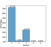
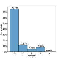
(a) Web dataset	(b) AdultContent dataset

Figure 1: Answer distribution of the real-world datasets

Distributions of worker answers. Figure 1 shows the answer distribution of the two real-world datasets. The analysis shows that the worker answer distribution of both datasets is skewed. In both Web and the AdultContent datasets, the ground truth of more than 72% tasks is value 0. Our analysis (Figure 1 (a) and (b)) shows that the majority of answers in theses two datasets are correct (i.e., the same as the ground truth). Furthermore, the remaining worker answers are distributed to a small number of values in a non-uniform fashion.

VI-C Parameter Impact on Truth Inference Accuracy

In this section, we present the impact of sparsity, data distribution, and data size on the accuracy of truth inference results.

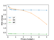
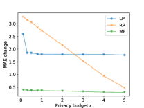
(a) sparsity$=0.9$	(b) sparsity$=0.5$

Figure 2: Accuracy of truth inference w.r.t. different privacy budget $\epsilon$ (2000 workers and 200 tasks).

Impact of privacy budget. First, we vary the privacy budget $\epsilon$, and measure MAE change of RR, LP, and MF. Figure 2 (a) - (b) show the results on the tasks whose truth follows the distribution $\mathcal{N}(0,1)$. Overall, MF always provides the smallest MAE change. The MAE change of LP witnesses a sudden drop when $\epsilon$ increases from 0.1 to 1, and keeps stable hereafter. This is because the Laplace noise is substantial when $\epsilon$ is small. On the other hand, the MAE change of RR keeps decreasing sharply with the growth of $\epsilon$. This is because according to Equation (8), when $\epsilon$ is as small as 0.1, $e^{\epsilon}\approx 1$. So the probability that RR keeps an answer unchanged is close to the probability that it substitutes the answer with a different random value in the domain. In other words, the perturbed answers are generated by following a uniform distribution. When $\epsilon$ increases, the existing values are much more likely to be kept in the dataset than being replaced. This leads to sharp drop of MAE change. Furthermore, when comparing Figure 2 (a) and (b), the MAE change of LP decreases when the sparsity goes down. This is because LP replace NULL values by following a uniform distribution over the domain [0,9] with the mean value 4.5, which is far from the center of answers 0. Thus, it leads to larger MAE change on sparse data. In the contrast, MF is not affected by the change of sparsity. This is consistent with our theoretical analysis.

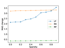
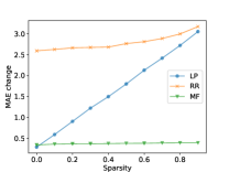
(a) $\epsilon=0.1$	(b) $\epsilon=1.0$

Figure 3: Accuracy of truth inference w.r.t. different data sparsity (2000 workers and 200 tasks)

Impact of data sparsity. We measure the MAE change of the three mechanisms under various answer sparsity and show the results in Figure 3. We observe that the MAE change of MF is very small in all settings. More importantly, it is insensitive to answer sparsity. In all cases, the MAE change never exceeds 0.5, even when the sparsity is as high as 0.9. This is because MF learns a latent joint distribution between the workers and tasks, and predicts the missing answers accurately. In comparison, the utility of LP and RR is sensitive to answer sparsity. Overall, the MAE change of these two approaches increases when the sparsity grows.

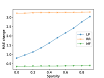
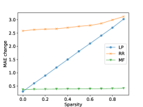
(a) $\epsilon=0.1$	(b) $\epsilon=1.0$

Figure 4: Accuracy of truth inference w.r.t. different data sparsity (10000 workers and 1000 tasks)

Impact of data size. We generate the datasets that consist of 10,000 workers and 1,000 tasks. The results for MAE change on the datasets with different sparsity are displayed in Figure 4. The observations are very similar to those on the small datasets (Figure 3). We highlight the most interesting observations. First, when $\epsilon=0.1$, the MAE change of LP is smaller when the data size is larger. LP requires to add the Laplace noise $Lap(\frac{|\Gamma|}{\epsilon})$ to each answer. The perturbation for each answer is large when $\epsilon=0.1$. However, for the same task, the average of the noise is inversely proportional to the number of answers. Therefore, when there are more answers, the aggregate noise from the workers reduces. We also notice that the MAE change resides in the same range for both small and large datasets. The reason is that the noise added to each answer is independent from the data size. We also vary the privacy budget $\epsilon$ on the large datasets and measure the MAE change. The results are similar to the small datasets (Figure 2). We include the results in the full paper [43].

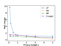
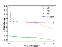
(a) Web dataset	(b) AdultContent dataset

Figure 5: Accuracy of truth inference w.r.t. privacy budget $\epsilon$ on two real-world datasets.

VI-D Comparison with Existing Method

We compare the MAE change of RR, LP, and MF with the 2-Layer approach [33] on the two real-world datasets. We vary the privacy budget $\epsilon$ and evaluate the MAE change of the four approaches. The results are shown in Figure 5. We have the following observations. First, similar to the results on the synthetic datasets, our MF approach has the lowest MAE change for most of the cases. By matrix factorization, the MF approach fills NULL values with non-NULL values that follow the current answer distribution. Therefore, the inferred truths from the perturbed answers are close to the inferred truths of the original data, which leads to a small MAE change. In contrast, by LP, RR, and 2-layer approaches, the NULL values are replaced with values in the range [0,4] with mean 2. Since the dataset is very sparse, such NULL value replacement shifts the inferred truth closer to 2 (compared with the inferred truth 0 from the original dataset), and thus further away from the ground truth. Therefore, the MAE change of these three approaches is larger than that of MF. Second, the 2-Layer approach shows comparable MAE change as RR. This is because it decides the privacy budget $\epsilon_{i}$ of each worker $W_{i}$ by following a uniform distribution with mean of $\epsilon$ and then perturbs the answers by following randomized response. Such data perturbation scheme introduces similar noise as RR, especially when the number of workers is large. Third, in the AdultContent dataset, the MAE change of the RR approach has a sharp drop when $\epsilon$ gets larger than 3. The reason is that, when $\epsilon$ gets larger than 3, RR keeps the NULL values unchanged with high probability (approximately $80\%$). The inferred truth on such perturbed dataset is very close to that from the original dataset, which leads to smaller MAE change.

VII Related Work

Differential privacy (DP) [16] is a privacy definition that requires the output of a computation should not allow inference about any record’s presence in or absence from the computation’s input. However, the classic DP model assumes the data curator is trusted. Therefore, it cannot be adapted to the crowdsourcing model in which the data curator is untrusted. Local differential privacy (LDP) has recently surfaced as a strong measure of privacy in contexts where personal information remains private even from data analysts. LDP has been widely used in practice. [19] propose RAPPOR to collect and analyze users’ data without privacy violation. RAPPOR is built on the concept of randomized response, which was proposed [48] initially for collection of survey answers. RAPPOR has been deployed in Google’s Chrome Web browser for reporting the statistics of users’ browsing history [12]. However, RAPPOR is limited to simple data analysis such as counting. It cannot deal with aggregates and sophisticated analysis such as classification and clustering [42]. Apple applies LDP to learn new words typed by users and identify frequently used Emojis while retaining user privacy [44]. Microsoft adapts LDP to its collection process of a variety of telemetry data [14]. A series of work [5, 4, 37, 46] aim to make LDP practical by improving the error of frequency estimation and heavy hitters on the data perturbed by LDP. Chen et al. [11] design a framework for aggregation of private location data with LDP. Since the same location is not equally sensitive to multiple users, the authors develop a personalized LDP protocol based on randomized response. Qin et al. [38] designed a protocol to reconstructed decentralized social networks by collecting neighbor lists from users while preserving LDP. Nyugen et al. [36] design an LDP mechanism named Harmony to collect and analyze data from users of smart devices. Harmony supports both basic statistics (e.g., mean and frequency estimates), and complex machine learning tasks (e.g., linear regression, logistic regression and SVM classification). Other works on LDP [19, 20, 37, 46] only focus on simple statistical aggregation functions, such as identifying heavy hitters and count estimation. None of these works consider truth inference as the utility function.

The problem of protecting worker privacy in crowdsourcing systems has received much attention recently. Kairouz et al. [26] investigate the trade-off between worker privacy and data utility as a constraint optimization problem, where the utility is measured as information theoretic statistics such as mutual information and divergence. They prove that solving the privacy-utility problem is equivalent to solving a finite dimensional linear program. Their utility measures are different from ours (truth inference). Ren et al. [39] consider the problem of publishing high-dimensional crowdsourced data with LDP. The server aggregates the data (in the format of randomized bit strings) from individual users and estimates their join distribution. Thus their utility function (i.e., estimation of joint distribution) is fundamentally different from ours. Among all the previous works, probably [33] is the most relevant to ours. The authors propose a two-layer perturbation mechanism based on randomized response to protect worker privacy, while providing high accuracy for truth discovery. However, [33] assumes that the data is complete. Béziaud et al. [6] protects worker profiles by allowing the workers to perturb their profiles locally by using randomized response. They do not consider truth inference as the utility function.

One research direction that is relevant to our work is to apply DP/LDP on recommender systems. The data-obfuscation solutions (e.g. [9, 40, 41]) adapts DP to the recommender systems and rely on adding noise to the original data or computation results to restrict the information leakage from recommender outputs. Shin et al. [42] focus on the LDP setting, aiming to protect both rating and item privacy for the users in recommendation systems. They develop a new matrix factorization algorithm under LDP. In specific, gradient perturbation is applied in the iterative factorization process. To reduce the perturbation error, the authors adopt random projection for matrix dimension reduction.

VIII Conclusion

In this paper, we consider the problem of privacy preserving Big data collection under the crowdsourcing setting, aiming to protecting worker privacy with LDP guarantee while providing highly accurate truth inference results. We overcome the weakness of two existing LDP approaches (namely randomized response and noise perturbation) due to worker answer sparsity, and design a new LDP matrix factorization method that adds perturbation on objective functions.

In the future, we plan to continue the study of privacy protection for crowdsourcing systems. We plan to design the privacy preservation method for other truth inference algorithms, for example, majority voting based methods [45]. We also plan to investigate how to protect task privacy, i.e., the sensitive information in the tasks, while allow the workers to provide high-quality answers.

References

- [1] Apple’s differential privacy is about collecting your data - but not your data. https://www.wired.com/2016/06/apples-differential-privacy-collecting-data/.
- [2] Ted cruz using firm that harvested data on millions of unwitting facebook users. https://www.theguardian.com/us-news/2015/dec/11/senator-ted-cruz-president-campaign-facebook-user-data.
- [3] R. Balu and T. Furon. Differentially private matrix factorization using sketching techniques. In Workshop on Information Hiding and Multimedia Security, pages 57–62. ACM, 2016.
- [4] R. Bassily and A. Smith. Local, private, efficient protocols for succinct histograms. In Symposium on Theory of Computing, pages 127–135. ACM, 2015.
- [5] R. Bassily, U. Stemmer, A. G. Thakurta, et al. Practical locally private heavy hitters. In Advances in Neural Information Processing Systems, pages 2285–2293, 2017.
- [6] L. Béziaud, T. Allard, and D. Gross-Amblard. Lightweight privacy-preserving task assignment in skill-aware crowdsourcing. In International Conference on Database and Expert Systems Applications, pages 18–26. Springer, 2017.
- [7] A. Bowser, A. Wiggins, L. Shanley, J. Preece, and S. Henderson. Sharing data while protecting privacy in citizen science. interactions, 21(1):70–73, 2014.
- [8] J. A. Burke, D. Estrin, M. Hansen, A. Parker, N. Ramanathan, S. Reddy, and M. B. Srivastava. Participatory sensing. 2006.
- [9] J. Canny. Collaborative filtering with privacy. In IEEE Symposium on Security and Privacy, pages 45–57, 2002.
- [10] C. C. Cao, J. She, Y. Tong, and L. Chen. Whom to ask?: jury selection for decision making tasks on micro-blog services. Proceedings of the VLDB Endowment, 5(11):1495–1506, 2012.
- [11] R. Chen, H. Li, A. Qin, S. P. Kasiviswanathan, and H. Jin. Private spatial data aggregation in the local setting. In International Conference on Data Engineering (ICDE), pages 289–300. IEEE, 2016.
- [12] Chromium.org. Design documents: Rappor (randomized aggregatable privacy preserving ordinal responses). http://www.chromium.org/developers/design-documents/rappor.
- [13] M. Ciglic, J. Eder, and C. Koncilia. k-anonymity of microdata with null values. In International Conference on Database and Expert Systems Applications, pages 328–342. Springer, 2014.
- [14] B. Ding, J. Kulkarni, and S. Yekhanin. Collecting telemetry data privately. In Advances in Neural Information Processing Systems, pages 3574–3583, 2017.
- [15] J. C. Duchi, M. I. Jordan, and M. J. Wainwright. Local privacy and statistical minimax rates. In IEEE Symposium on Foundations of Computer Science (FOCS), pages 429–438, 2013.
- [16] C. Dwork. Differential privacy. In the International Colloquium on Automata, Languages and Programming (ICALP), pages 1–12. Springer, 2006.
- [17] C. Dwork. Differential privacy: A survey of results. In International Conference on Theory and Applications of Models of Computation, pages 1–19. Springer, 2008.
- [18] C. Dwork, F. McSherry, K. Nissim, and A. Smith. Calibrating noise to sensitivity in private data analysis. In Theory of Cryptography, pages 265–284. Springer, 2006.
- [19] Ú. Erlingsson, V. Pihur, and A. Korolova. Rappor: Randomized aggregatable privacy-preserving ordinal response. In International Conference on Computer and Communications Security, pages 1054–1067, 2014.
- [20] G. Fanti, V. Pihur, and Ú. Erlingsson. Building a rappor with the unknown: Privacy-preserving learning of associations and data dictionaries. Proceedings on Privacy Enhancing Technologies, 2016(3):41–61, 2016.
- [21] A. Friedman, S. Berkovsky, and M. A. Kaafar. A differential privacy framework for matrix factorization recommender systems. User Modeling and User-Adapted Interaction, 26(5):425–458, 2016.
- [22] S. Guo, A. Parameswaran, and H. Garcia-Molina. So who won?: dynamic max discovery with the crowd. In International Conference on Management of Data, pages 385–396, 2012.
- [23] M. Hay, A. Machanavajjhala, G. Miklau, Y. Chen, and D. Zhang. Principled evaluation of differentially private algorithms using dpbench. In International Conference on Management of Data, pages 139–154. ACM, 2016.
- [24] J. Hua, C. Xia, and S. Zhong. Differentially private matrix factorization. In IJCAI, pages 1763–1770, 2015.
- [25] A. Inc. Amazon mechanical turk. https://www.mturk.com/mturk.
- [26] P. Kairouz, S. Oh, and P. Viswanath. Extremal mechanisms for local differential privacy. In Advances in Neural Information Processing Systems, pages 2879–2887, 2014.
- [27] T. Kandappu, A. Friedman, V. Sivaraman, and R. Boreli. Privacy in crowdsourced platforms. In Privacy in a Digital, Networked World, pages 57–84. 2015.
- [28] V. Karwa, A. B. Slavković, and P. Krivitsky. Differentially private exponential random graphs. In International Conference on Privacy in Statistical Databases, pages 143–155. Springer, 2014.
- [29] S. P. Kasiviswanathan, H. K. Lee, K. Nissim, S. Raskhodnikova, and A. Smith. What can we learn privately? SIAM Journal on Computing, 40(3):793–826, 2011.
- [30] Y. Koren, R. Bell, and C. Volinsky. Matrix factorization techniques for recommender systems. Computer, 42(8), 2009.
- [31] H. Li, L. Xiong, L. Zhang, and X. Jiang. Dpsynthesizer: differentially private data synthesizer for privacy preserving data sharing. Proceedings of the VLDB Endowment, 7(13):1677–1680, 2014.
- [32] Q. Li, Y. Li, J. Gao, L. Su, B. Zhao, M. Demirbas, W. Fan, and J. Han. A confidence-aware approach for truth discovery on long-tail data. Proceedings of the VLDB Endowment, 8(4):425–436, 2014.
- [33] Y. Li, C. Miao, L. Su, J. Gao, Q. Li, B. Ding, and K. Ren. An efficient two-layer mechanism for privacy-preserving truth discovery. In International Conference on Knowledge Discovery and Data Mining, 2018.
- [34] X. Liu, M. Lu, B. C. Ooi, Y. Shen, S. Wu, and M. Zhang. Cdas: a crowdsourcing data analytics system. Proceedings of the VLDB Endowment, 5(10):1040–1051, 2012.
- [35] N. Mohammed, R. Chen, B. C. Fung, and P. S. Yu. Differentially private data release for data mining. In Proceedings of the 17th ACM SIGKDD International Conference on Knowledge Discovery and Data Mining, pages 493–501, 2011.
- [36] T. T. Nguyên, X. Xiao, Y. Yang, S. C. Hui, H. Shin, and J. Shin. Collecting and analyzing data from smart device users with local differential privacy. arXiv preprint arXiv:1606.05053, 2016.
- [37] Z. Qin, Y. Yang, T. Yu, I. Khalil, X. Xiao, and K. Ren. Heavy hitter estimation over set-valued data with local differential privacy. In ACM Conference on Computer and Communications Security, pages 192–203. ACM, 2016.
- [38] Z. Qin, T. Yu, Y. Yang, I. Khalil, X. Xiao, and K. Ren. Generating synthetic decentralized social graphs with local differential privacy. In ACM Conference on Computer and Communications Security, pages 425–438. ACM, 2017.
- [39] X. Ren, C.-M. Yu, W. Yu, S. Yang, X. Yang, J. A. McCann, and S. Y. Philip. Lopub: High-dimensional crowdsourced data publication with local differential privacy. Transactions on Information Forensics and Security, 13(9):2151–2166, 2018.
- [40] Y. Shen and H. Jin. Privacy-preserving personalized recommendation: An instance-based approach via differential privacy. In International Conference on Data Mining (ICDM), pages 540–549. IEEE, 2014.
- [41] Y. Shen and H. Jin. Epicrec: Towards practical differentially private framework for personalized recommendation. In International Conference on Computer and Communications Security, pages 180–191. ACM, 2016.
- [42] H. Shin, S. Kim, J. Shin, and X. Xiao. Privacy enhanced matrix factorization for recommendation with local differential privacy. Transactions on Knowledge and Data Engineering, 2018.
- [43] H. Sun, B. Dong, and H. W. Wang. Truth inference on sparse crowdsourcing data with local differentially privacy. http://dmlab.cs.stevens.edu/publications?name=truth-inference-sparse, 2018.
- [44] A. G. Thakurta, A. H. Vyrros, U. S. Vaishampayan, G. Kapoor, J. Freudiger, V. R. Sridhar, and D. Davidson. Learning new words, 2017. US Patent 9,594,741.
- [45] T. Tian and J. Zhu. Max-margin majority voting for learning from crowds. In Advances in Neural Information Processing Systems, pages 1621–1629, 2015.
- [46] T. Wang, J. Blocki, N. Li, and S. Jha. Locally differentially private protocols for frequency estimation. In Proc. of the 26th USENIX Security Symposium, pages 729–745, 2017.
- [47] Y. Wang, X. Wu, and D. Hu. Using randomized response for differential privacy preserving data collection. In EDBT/ICDT Workshops, 2016.
- [48] S. L. Warner. Randomized response: A survey technique for eliminating evasive answer bias. Journal of the American Statistical Association, 60(309):63–69, 1965.
- [49] X. Xiao, G. Wang, and J. Gehrke. Differential privacy via wavelet transforms. IEEE Transactions on Knowledge and Data Engineering, 23(8):1200–1214, 2011.
- [50] C. J. Zhang, L. Chen, H. Jagadish, and C. C. Cao. Reducing uncertainty of schema matching via crowdsourcing. Proceedings of the VLDB Endowment, 6(9):757–768, 2013.
- [51] B. Zhao and J. Han. A probabilistic model for estimating real-valued truth from conflicting sources. International Workshop on Quality in Databases, 2012.