An explicit divergence-free DG method for incompressible magnetohydrodynamics

Abstract.

We extend the recently introduced explicit divergence-free DG scheme for incompressible hydrodynamics [Fu18c] to the incompressible magnetohydrodynamics (MHD). A globally divergence-free finite element space is used for both the velocity and the magnetic field. Highlights of the scheme includes global and local conservation properties, high-order accuracy, energy-stability, pressure-robustness. When forward Euler time stepping is used, we need two symmetric positive definite (SPD) hybrid-mixed Poisson solvers (one for velocity and one for magnetic field) to advance the solution to the next time level.

Since we treat both viscosity in the momentum equation and resistivity in the magnetic induction equation explicitly, the method shall be best suited for inviscid or high-Reynolds number, low resistivity flows so that the CFL constraint is not too restrictive.

1. Introduction

The search for finite element methods that produce an exactly divergence-free velocity field for incompressible hydrodynamics has regained considerable interest in the past decade; see e.g. the recent review article [John17]. Equally well, the enforcement of the divergence-free constraint for the magnetic field in magnetohydrodynamics (MHD) is a long standing computational issue in numerical simulations, see e.g. [Brackbill80, Toth, Dedner02].

In this paper, we propose a divergence-free DG method for the incompressible MHD equation based on a velocity-magnetic field formulation, extending our previous work on a divergence-free DG scheme for incompressible hydrodynamics [Fu18c] to the incompressible MHD setting. In particular, we use a globally divergence-free finite element space for both the velocity and magnetic field. Hence, the pressure field and the divergence-free constraints in the equations are eliminated by design. The scheme enjoys features such as global and local conservation properties, high-order accuracy, energy-stability, and pressure-robustness. Moreover, the scheme can be efficiently implemented [Fu18c] when coupled with explicit time stepping methods. In particular, two hybrid-mixed Poisson solvers (equivalent to the mass matrix inversion of the divergence-free finite elements) is needed to advance solution in time when forward Euler time stepping is used.

We point out that while it is usually agreed that a Poisson solver for the evolution of velocity in incompressible flow is unavoidable, this might not be the case for the evolution of the magnetic field. Indeed, when complete local finite element spaces were used for the magnetic field, e.g. the locally divergence-free DG method [LiShu05], explicit time stepping yields the inversion of a block-diagonal mass matrix, hence, the Poisson solver for the magnetic field is avoided. However, such method does not provide an exactly divergence-free magnetic field due to the lack of $H(\mathrm{div})$-conformity, and reconstructing an exactly divergence-free magnetic field usually requires, again, a Poisson solver [Brackbill80]. However, we particularly mention that the constraint transport (CT) method [CT] produces an exactly divergence-free magnetic field without the need of a global solver. We refer to the discussion in [Toth] for a comparison of various version of CT methods. See also the recent work on global divergence-free DG methods for compressible MHD [Li12, Fu2018], which can be interpreted as high-order CT-type methods. The key idea to achieve a divergence-free magnetic field for the CT methods is to first advance in time the normal component of the magnetic field on the mesh interfaces, then apply a (locally defined) divergence-free reconstruction procedure. It seems that such CT procedure is not available yet for the velocity evolution for incompressible flow. For this reason, we chose to use the same Poisson-solver approach for the magnetic field evolution as that for the velocity evolution. Our approach leads to a remarkably simple formulation which is provable energy stable in the semi-discrete case. Moreover, its implementation can be trivially adapted from an existing explicit divergence-free DG code for incompressible hydrodynamics.

The rest of the paper is organized as follows. In Section 2, the explicit divergence-free DG scheme is introduced for the incompressible inviscid MHD equations. It is extended to the incompressible viscous MHD equations in Section 3. Two dimensional numerical results are presented in Section 4. Finally, we conclude in Section 5.

2. Incompressible inviscid MHD

We consider the following incompressible inviscid MHD equations in conservative form:

$$\partial_{t}\boldsymbol{u}+{\nabla\cdot}(\boldsymbol{u}\otimes\boldsymbol{u}-\boldsymbol{B}\otimes\boldsymbol{B})+\nabla(p+\frac{1}{2}\boldsymbol{B}\cdot\boldsymbol{B})= \;0, \text{ in }\Omega,$$ (1a)

$${\nabla\cdot}\boldsymbol{u}= \;0, \text{ in }\Omega,$$ (1b)

$$\partial_{t}\boldsymbol{B}+{\nabla\cdot}(\boldsymbol{u}\otimes\boldsymbol{B}-\boldsymbol{B}\otimes\boldsymbol{u})= \;0, \text{ in }\Omega.$$ (1c)

with initial condition

$$\boldsymbol{u}(x,0)=\boldsymbol{u}_{0}(x),\quad\boldsymbol{B}(x,0)=\boldsymbol{B}_{0}(x),\quad\forall x\in\Omega,$$

where $\boldsymbol{u}$ is the velocity, $p$ is the pressure , and $\boldsymbol{B}$ is the magnetic field, $\Omega\subset\mathbb{R}^{d}$(d=2,3) is a polygonal/polyhedral domain. The initial velocity and magnetic field $\boldsymbol{u}_{0}(x)$ and $\boldsymbol{B}_{0}(x)$ are assumed to be divergence-free. For simplicity, we consider periodic boundary conditions only. However, the inflow/outflow/wall boundary conditions can be easily included, see [Fu18c].

We spefically mention that taking divergence of the equation (1c) yields

$$\partial_{t}({\nabla\cdot}\boldsymbol{B})=0.$$

This implies that the ${\nabla\cdot}\boldsymbol{B}=0$ condition will always be respected since the initial magnetic field satisfies ${\nabla\cdot}\boldsymbol{B}_{0}=0$. The physical interpretation of this identity is that there exists no magnetic monopoles.

2.1. Preliminaries

Let ${\mathcal{T}_{h}}$ be a conforming simplicial triangulation of $\Omega$. For any element $T\in{\mathcal{T}_{h}}$, we denote by $h_{T}$ its diameter and we denote by $h$ the maximum diameter over all mesh elements. Denote by $\mathcal{F}_{h}$ the set of facets of ${\mathcal{T}_{h}}$.

The following finite element space will be used to discretize both the velocity and magnetic field:

$$\boldsymbol{V}_{\!h}^{k,-1}:= \;\{\boldsymbol{v}\in\Pi_{T\in{\mathcal{T}_{h}}}[\mathbb{P}^{k}(T)]^{d},\;\;[\![\boldsymbol{v}_{T}\cdot\boldsymbol{n}]\!]_{F}=0\;\;\forall F\in\mathcal{F}_{h},\quad{\nabla\cdot}\boldsymbol{v}=0\text{ on }{\mathcal{T}_{h}}.\}$$ (2)

where the polynomial degree $k\geq 1$, and $[\![\cdot]\!]$ is the usual jump operator and $\mathbb{P}^{k}$ the space of polynomials up to degree $k$. Notice that the space $\boldsymbol{V}_{\!h}^{k,-1}\subset H(\mathrm{div},\Omega)$ is not a standard finite element space in the sense that no local bases exist due to the divergence-free constraint. We introduce proper Lagrange multipliers for the implementation of our scheme using such space, see details in [Fu18c, Section 2.4]; see also Remark 1 below.

Finally, we introduce the jump and average notation. Let $\boldsymbol{\phi}_{h}$ be any function in $\boldsymbol{V}_{\!h}^{k,-1}$. On each facet $F\in\mathcal{F}_{h}$ shared by two elements $K^{-}$ and $K^{+}$, we denote $(\boldsymbol{\phi}_{h})^{\pm}|_{F}=\left.(\boldsymbol{\phi}_{h})\right|_{K^{\pm}}$, and use

$$[\![{\boldsymbol{\phi}_{h}}]\!]|_{F}=\boldsymbol{\phi}_{h}^{+}-\boldsymbol{\phi}_{h}^{-},\quad\quad\{\!\!\{{\boldsymbol{\phi}_{h}}\}\!\!\}|_{F}=\frac{1}{2}(\boldsymbol{\phi}_{h}^{+}+\boldsymbol{\phi}_{h}^{-})$$ (3)

to denote the jump and the average of $\boldsymbol{\phi}_{h}$. Here $K^{-}$ is chosen such that $F$ is an outflow facet based on the velocity field $\boldsymbol{u}_{h}$, i.e. $\boldsymbol{u}_{h}\cdot\boldsymbol{n}^{-}\geq 0$ where $\boldsymbol{n}^{-}$ is the normal direction of $K^{-}$ on $F$. Note that the jump term only contains jump for the tangential component of the vector $\boldsymbol{\phi}_{h}$ due to normal continuity of the finite element space.

2.2. Spatial discretization

The divergence-free space $\boldsymbol{V}_{\!h}^{k,-1}$ shall be used for both the velocity and magnetic field. With this space in use, the divergence-free constraint (1b) is point-wisely satisfied by design, and the (total) pressure gradient term in (1a) do not enter into the weak formulation of the scheme. Using standard upwinding DG discretizations for the four convective terms

$${\nabla\cdot}(\boldsymbol{u}\otimes\boldsymbol{u}),\;\;{\nabla\cdot}(\boldsymbol{B}\otimes\boldsymbol{B}),\;\;{\nabla\cdot}(\boldsymbol{u}\otimes\boldsymbol{B}),\;\;{\nabla\cdot}(\boldsymbol{B}\otimes\boldsymbol{u}),$$ (4)

we arrive at the following semi-discrete scheme: find $(\boldsymbol{u}_{h}(t),\boldsymbol{B}_{h}(t))\in\boldsymbol{V}_{\!h}^{k,-1}\times\boldsymbol{V}_{\!h}^{k,-1}$ such that

$$(\partial_{t}\boldsymbol{u}_{h},\boldsymbol{v}_{h})_{{\mathcal{T}_{h}}}+\mathcal{C}_{uu}(\boldsymbol{u}_{h};\boldsymbol{u}_{h},\boldsymbol{v}_{h})-\mathcal{C}_{bb}(\boldsymbol{B}_{h};\boldsymbol{B}_{h},\boldsymbol{v}_{h})= 0,\quad\forall\boldsymbol{v}_{h}\in\boldsymbol{V}_{\!h}^{k,-1},$$ (5a)

$$(\partial_{t}\boldsymbol{B}_{h},\boldsymbol{\phi}_{h})_{{\mathcal{T}_{h}}}+\mathcal{C}_{ub}(\boldsymbol{u}_{h};\boldsymbol{B}_{h},\boldsymbol{\phi}_{h})-\mathcal{C}_{bu}(\boldsymbol{B}_{h};\boldsymbol{u}_{h},\boldsymbol{\phi}_{h})= 0,\quad\forall\boldsymbol{\phi}_{h}\in\boldsymbol{V}_{\!h}^{k,-1}.$$ (5b)

where $$(\cdot,\cdot)_{\mathcal{T}_{h}} L^{2}$$ denotes the standard -inner product, and the four convective operators are given below

$$\mathcal{C}_{uu}(\boldsymbol{u}_{h};\boldsymbol{u}_{h},\boldsymbol{v}_{h}):= \sum_{T\in{\mathcal{T}_{h}}}\int_{T}-(\boldsymbol{u}_{h}\otimes\boldsymbol{u}_{h}):{\nabla}\boldsymbol{v}_{h}\,\mathrm{dx}+\int_{\partial T}(\boldsymbol{u}_{h}\cdot\boldsymbol{n})({\boldsymbol{u}}_{h}^{-}\cdot\boldsymbol{v}_{h})\,\mathrm{ds}$$

$$\mathcal{C}_{bb}(\boldsymbol{B}_{h};\boldsymbol{B}_{h},\boldsymbol{v}_{h}):= \sum_{T\in{\mathcal{T}_{h}}}\int_{T}-(\boldsymbol{B}_{h}\otimes\boldsymbol{B}_{h}):{\nabla}\boldsymbol{v}_{h}\,\mathrm{dx}+\int_{\partial T}(\boldsymbol{B}_{h}\cdot\boldsymbol{n})(\widehat{\boldsymbol{B}}_{h}\cdot\boldsymbol{v}_{h})\,\mathrm{ds}$$

$$\mathcal{C}_{ub}(\boldsymbol{u}_{h};\boldsymbol{B}_{h},\boldsymbol{\phi}_{h}):= \sum_{T\in{\mathcal{T}_{h}}}\int_{T}-(\boldsymbol{u}_{h}\otimes\boldsymbol{B}_{h}):{\nabla}\boldsymbol{\phi}_{h}\,\mathrm{dx}+\int_{\partial T}(\boldsymbol{u}_{h}\cdot\boldsymbol{n})({\boldsymbol{B}}_{h}^{-}\cdot\boldsymbol{v}_{h})\,\mathrm{ds}$$

$$\mathcal{C}_{bu}(\boldsymbol{B}_{h};\boldsymbol{u}_{h},\boldsymbol{\phi}_{h}):= \sum_{T\in{\mathcal{T}_{h}}}\int_{T}-(\boldsymbol{B}_{h}\otimes\boldsymbol{u}_{h}):{\nabla}\boldsymbol{\phi}_{h}\,\mathrm{dx}+\int_{\partial T}(\boldsymbol{B}_{h}\cdot\boldsymbol{n})(\widehat{\boldsymbol{u}}_{h}\cdot\boldsymbol{\phi}_{h})\,\mathrm{ds},$$

where the four upwinding numerical fluxes are given as follows:

$$\boldsymbol{u}_{h}^{-}|_{F}= \boldsymbol{u}_{h}|_{K^{-}},\quad \quad\boldsymbol{B}_{h}^{-}|_{F}=\boldsymbol{B}_{h}|_{K^{-}},$$ (6)

$$\widehat{\boldsymbol{u}}_{h}|_{F}= \{\!\!\{{\boldsymbol{u}_{h}}\}\!\!\}+\frac{1}{2}s_{F}[\![{\boldsymbol{B}_{h}}]\!], \quad\widehat{\boldsymbol{B}}_{h}|_{F}=\{\!\!\{{\boldsymbol{B}_{h}}\}\!\!\}+\frac{1}{2}s_{F}[\![{\boldsymbol{u}_{h}}]\!],$$ (7)

where $s_{F}$ takes value $1$ if $(\boldsymbol{B}_{h}\cdot\boldsymbol{n})(\boldsymbol{u}_{h}\cdot\boldsymbol{n})|_{F}>0$, and $-1$ if $(\boldsymbol{B}_{h}\cdot\boldsymbol{n})(\boldsymbol{u}_{h}\cdot\boldsymbol{n})|_{F}\leq 0$. Notice that the numerical fluxes $\boldsymbol{u}_{h}^{-}$ and $\boldsymbol{B}_{h}^{-}$ are the upwinding fluxes based on the velocity direction $\boldsymbol{u}_{h}\cdot\boldsymbol{n}$, whilst the numerical fluxes $\widehat{\boldsymbol{u}}_{h}$ and $\widehat{\boldsymbol{B}}_{h}$ are the upwinding fluxes based on the magnetic field direction $\boldsymbol{B}_{h}\cdot\boldsymbol{n}$. A simple calculation yields

$$\mathcal{C}_{uu}(\boldsymbol{u}_{h};\boldsymbol{u}_{h},\boldsymbol{u}_{h})=\frac{1}{2}\sum_{F\in\mathcal{F}_{h}}\int_{F}|\boldsymbol{u}_{h}\cdot\boldsymbol{n}|[\![{\boldsymbol{u}_{h}}]\!]^{2}\,\mathrm{ds} \geq 0,$$

$$\mathcal{C}_{ub}(\boldsymbol{u}_{h};\boldsymbol{B}_{h},\boldsymbol{B}_{h})=\frac{1}{2}\sum_{F\in\mathcal{F}_{h}}\int_{F}|\boldsymbol{u}_{h}\cdot\boldsymbol{n}|[\![{\boldsymbol{B}_{h}}]\!]^{2}\,\mathrm{ds} \geq 0,$$

$$\mathcal{C}_{bb}(\boldsymbol{B}_{h};\boldsymbol{B}_{h},\boldsymbol{u}_{h})+\mathcal{C}_{bu}(\boldsymbol{B}_{h};\boldsymbol{u}_{h},\boldsymbol{B}_{h}){\color[rgb]{1,1,1}xxxxxxxxxxx}$$

$$=-\frac{1}{2}\sum_{F\in\mathcal{F}_{h}}\int_{F}|\boldsymbol{B}_{h}\cdot\boldsymbol{n}|\left[[\![{\boldsymbol{u}_{h}}]\!]^{2}+[\![{\boldsymbol{B}_{h}}]\!]^{2}\right]\,\mathrm{ds} \leq 0.$$

Hence, a standard energy argument implies that the scheme (5) is energy-stable in the sense that the total energy do not increase:

$$\partial_{t}\Big{(}(\boldsymbol{u}_{h},\boldsymbol{u}_{h})_{\mathcal{T}_{h}}+(\boldsymbol{B}_{h},\boldsymbol{B}_{h})_{\mathcal{T}_{h}}\Big{)}$$

$$=\sum_{F\in\mathcal{F}_{h}}\int_{F}(|\boldsymbol{u}_{h}\cdot\boldsymbol{n}|+|\boldsymbol{B}_{h}\cdot\boldsymbol{n}|)\left([\![{\boldsymbol{u}_{h}}]\!]^{2}+[\![{\boldsymbol{B}_{h}}]\!]^{2}\right)\,\mathrm{ds}\leq 0.$$ (8)

2.3. Temporal discretization

The semi-discrete scheme (5) can be written as

$$\mathcal{M}(\partial_{t}\boldsymbol{U}_{h})=\mathcal{L}(\boldsymbol{U}_{h}),$$ (9)

where $\mathcal{M}$ is the $2\times 2$ block-diagonal mass matrix for the compound space $\boldsymbol{V}_{\!h}^{k,-1}\times\boldsymbol{V}_{\!h}^{k,-1}$, and $\mathcal{L}(\cdot)$ the spatial discretization operator, with $\boldsymbol{U}_{h}$ includes unknowns for both $\boldsymbol{u}_{h}$ and $\boldsymbol{B}_{h}$. Any explicit time stepping techniques can be applied to the ODE system (9). We use the following three-stage, third-order strong-stability preserving Runge-Kutta method (TVD-RK3) [ShuOsher88] in our numerical experiments:

$$\mathcal{M}\boldsymbol{U}_{h}^{(1)}= \;\mathcal{M}\boldsymbol{U}_{h}^{n}+\Delta t^{n}\mathcal{L}(\boldsymbol{U}_{h}^{n}),$$

$$\mathcal{M}\boldsymbol{U}_{h}^{(2)}= \;\frac{3}{4}\mathcal{M}\boldsymbol{U}_{h}^{n}+\frac{1}{4}\left[\mathcal{M}\boldsymbol{U}_{h}^{(1)}+\Delta t^{n}\mathcal{L}(\boldsymbol{U}_{h}^{(1)})\right],$$ (10)

$$\mathcal{M}\boldsymbol{u}_{h}^{n+1}= \;\frac{1}{3}\mathcal{M}\boldsymbol{U}_{h}^{n}+\frac{2}{3}\left[\mathcal{M}\boldsymbol{U}_{h}^{(2)}+\Delta t^{n}\mathcal{L}(\boldsymbol{U}_{h}^{(2)})\right],$$

where $\boldsymbol{U}_{h}^{n}$ is the given solution at time level $t^{n}$ and $\boldsymbol{U}_{h}^{n+1}$ is the computed solution at time level $t^{n+1}=t^{n}+\Delta t^{n}$. In each time step, $3\times 2=6$ inversion of the mass matrix for the divergence-free space $\boldsymbol{V}_{\!h}^{k,-1}$ are needed. Hence, the computational cost is essentially doubled per time step comparing with a corresponding hydrodynamic simulation.

Remark 1 (Implementation).

The actual implementation of the scheme (2.3) that avoids global mass matrix inversion was discussed in details in [Fu18c] where appropriate Lagrange multipliers were introduced. In particular, it was shown in [Fu18c, Section 2.4] that the inversion of the mass matrix is equivalent to a (symmetric-positive-definite) hybrid-mixed Poisson solver.

3. Incompressible viscous MHD

Now, we extend the scheme (5) to the following incompressible, viscous, resistive MHD equations:

$$\partial_{t}\boldsymbol{u}+{\nabla\cdot}(\boldsymbol{u}\otimes\boldsymbol{u}-\boldsymbol{B}\otimes\boldsymbol{B})+\nabla(p+\frac{1}{2}\|\boldsymbol{B}\|^{2})-\nu\triangle\boldsymbol{u}= \;0, \text{ in }\Omega,$$ (11a)

$${\nabla\cdot}\boldsymbol{u}= \;0, \text{ in }\Omega,$$ (11b)

$$\partial_{t}\boldsymbol{B}+{\nabla\cdot}(\boldsymbol{u}\otimes\boldsymbol{B}-\boldsymbol{B}\otimes\boldsymbol{u})-\eta\triangle\boldsymbol{B}= \;0, \text{ in }\Omega,$$ (11c)

with divergence-free initial conditions

$$\boldsymbol{u}(x,0)=\boldsymbol{u}_{0}(x),\;\;\boldsymbol{B}(x,0)=\boldsymbol{B}_{0}(x)\quad\forall x\in\Omega,$$

and periodic boundary conditions. Here $\nu=1/\mathrm{Re}$ is the viscosity, and $\eta$ is the resistivity.

We discretize both viscous and resistive terms using a symmetric interior penalty DG method [ArnoldBrezziCockburnMarini02]. The semi-discrete scheme reads as follows: find $\boldsymbol{u}_{h}(t)\in\boldsymbol{V}_{\!h}^{k,-1}$ such that

$$(\partial_{t}\boldsymbol{u}_{h},\boldsymbol{v}_{h})_{{\mathcal{T}_{h}}}+\mathcal{C}_{uu}(\boldsymbol{u}_{h};\boldsymbol{u}_{h},\boldsymbol{v}_{h})$$

$$\;\;\;\;-\mathcal{C}_{bb}(\boldsymbol{B}_{h};\boldsymbol{B}_{h},\boldsymbol{v}_{h})+\nu\mathcal{A}_{d}(\boldsymbol{u}_{h},\boldsymbol{v}_{h}) =0,\quad\forall\boldsymbol{v}_{h}\in\boldsymbol{V}_{\!h}^{k,-1},$$ (12a)

$$(\partial_{t}\boldsymbol{B}_{h},\boldsymbol{\phi}_{h})_{{\mathcal{T}_{h}}}+\mathcal{C}_{ub}(\boldsymbol{u}_{h};\boldsymbol{B}_{h},\boldsymbol{\phi}_{h})$$

$$\;\;\;\;-\mathcal{C}_{bu}(\boldsymbol{B}_{h};\boldsymbol{u}_{h},\boldsymbol{\phi}_{h})+\eta\mathcal{A}_{d}(\boldsymbol{B}_{h},\boldsymbol{\phi}_{h}) =0,\quad\forall\boldsymbol{\phi}_{h}\in\boldsymbol{V}_{\!h}^{k,-1}.$$ (12b)

where the bilinear form for the diffusion term, $\mathcal{A}_{d}$, takes the following form

$$\mathcal{A}_{d}(\boldsymbol{u}_{h},\boldsymbol{v}_{h}):= \;\sum_{T\in{\mathcal{T}_{h}}}\int_{T}\nabla u:\nabla v\,\mathrm{dx}$$

$$-\sum_{F\in\mathcal{F}_{h}}\int_{F}\{\!\!\{{\nabla\boldsymbol{u}_{h}}\}\!\!\}[\![{\boldsymbol{v}_{h}\otimes\boldsymbol{n}}]\!]\,\mathrm{ds}$$

$$-\sum_{F\in\mathcal{F}_{h}}\int_{F}\{\!\!\{{\nabla\boldsymbol{v}_{h}}\}\!\!\}[\![{\boldsymbol{u}_{h}\otimes\boldsymbol{n}}]\!]\,\mathrm{ds}$$

$$+\sum_{F\in\mathcal{F}_{h}}\int_{F}\frac{\alpha k^{2}}{h}[\![{\boldsymbol{u}_{h}\otimes\boldsymbol{n}}]\!][\![{\boldsymbol{v}_{h}\otimes\boldsymbol{n}}]\!]\,\mathrm{ds},$$ (13)

with $\alpha>0$ a sufficiently large stabilization constant. We take $\alpha=2$ in the numerics presented in the next section.

To obtain a fully discrete scheme, we use the same explicit stepping as the inviscid case. A standard CFL time stepping restriction $\Delta t\leq C\min\{h/v_{\max},h^{2}/\max\{\nu,\eta\}\}$ is to be expected, where $v_{\max}$ is the maximum velocity speed. Hence, the method shall be applied to high Reynolds number, low resistivity flows where $\max\{\nu,\eta\}\ll 1$ to avoid severe time stepping restrictions.

Finally, we point out that when either $\nu$ or $\eta$ is not too small, one shall consider treating viscous/resistive terms implicitly to avoid parabolic time stepping. Hence, a Stokes solver is needed. In that setting, an hybridizable discontinuous Galerkin (HDG) discretization [CockburnGopalakrishnanLazarov09] of the diffusion operator is more favorable in terms of the linear system solver efficiency; see some discussion on divergence-free HDG schemes for incompressible flow in [Lehrenfeld:10, LehrenfeldSchoberl16].

4. Numerical results

In this section, we present some numerical tests in two dimensions to show the performance of our scheme. The numerical results are performed using the NGSolve software [Schoberl16]. For the viscous operator (3), we take the stabilization parameter $\alpha$ to be $2$. We use the TVD-RK3 time stepping (2.3) with sufficiently small time step size that ensure stability

$$\Delta t\leq\min\left\{C\!F\!L_{\mathrm{conv}}h/v_{\max},C\!F\!L_{\mathrm{visc}}h^{2}/\max\{\nu,\eta\}\right\},$$

where $C\!F\!L_{\mathrm{conv}}$ and $C\!F\!L_{\mathrm{visc}}$ are the CFL stability constants depending on the polynomial degree $k$. We use a pre-factored sparse-Cholesky factorization for the hybrid-mixed Poisson solver that is needed in each time step.

Example 1: Accuracy test

This example is used to check the accuracy of our schemes, both for the inviscid MHD equations (1) and for the viscous, ideal MHD equations (11) with $\nu=1/Re=1/100$, $\eta=0$. We take the domain to be $[0,2\pi]\times[0,2\pi]$ and use a periodic boundary condition. The initial condition and source term are chosen such that the exact solution is

$$u_{1}=B_{1}=-\cos(x)\sin(y)\exp(-2t/\mathrm{Re}),u_{2}=B_{2}=\sin(x)\cos(y)\exp(-2t/\mathrm{Re}).$$

The $L^{2}$-errors in velocity and magnetic field at $t=0.5$ on unstructured triangular meshes are shown in Table 1. It is clear to observe optimal $(k+1)$-th order of convergence for both variables in both cases.

Table 1. History of convergence of the $L^{2}$ errors in velocity $\boldsymbol{u}_{h}$and magnetic field $\boldsymbol{B}_{h}$ at time $t=1$.

		inviscid MHD				viscous, ideal MHD ($\mathrm{Re}=100$)
$k$	$h$	$\boldsymbol{u}_{h}$-error	order	$\boldsymbol{B}_{h}$-error	order	$\boldsymbol{u}_{h}$-error	order	$\boldsymbol{B}_{h}$-error	order
1	0.7854	1.853e-01	0.00	1.853e-01	0.00	1.824e-01	-1.82	1.850e-01	4.57
	0.3927	4.119e-02	2.17	4.119e-02	2.17	4.043e-02	2.17	4.111e-02	2.17
	0.1963	1.010e-02	2.03	1.010e-02	2.03	9.892e-03	2.03	1.005e-02	2.03
	0.0982	2.463e-03	2.04	2.463e-03	2.04	2.414e-03	2.03	2.444e-03	2.04
2	0.7854	2.280e-02	0.00	2.280e-02	0.00	2.191e-02	0.00	2.256e-02	0.00
	0.3927	2.783e-03	3.03	2.783e-03	3.03	2.500e-03	3.13	2.622e-03	3.10
	0.1963	3.641e-04	2.93	3.641e-04	2.93	2.920e-04	3.10	3.166e-04	3.05
	0.0982	4.554e-05	3.00	4.554e-05	3.00	3.196e-05	3.19	3.698e-05	3.10
3	0.7854	1.223e-03	0.00	1.223e-03	0.00	1.218e-03	0.00	1.239e-03	0.00
	0.3927	6.555e-05	4.22	6.555e-05	4.22	6.888e-05	4.14	7.122e-05	4.12
	0.1963	4.242e-06	3.95	4.242e-06	3.95	4.693e-06	3.88	4.955e-06	3.85
	0.0982	2.592e-07	4.03	2.592e-07	4.03	2.802e-07	4.07	2.976e-07	4.06

Example 2: Orszag-Tang vortex problem

We consider the Orszag-Tang vortex problem [orszag1979]. The inviscid equation (1) on the domain $[0,2\pi]\times[0,2\pi]$ with a periodic boundary condition and an initial condition:

$$u_{1}(x,y,0)=-\sin(y)\quad u_{2}(x,y,0)=\sin(x),$$ (14)

$$B_{1}(x,y,0)=-\sin(y)\quad B_{2}(x,y,0)=\sin(2x),$$ (15)

is solved.

We use $P^{3}$ approximation on two unstructured triangular meshes with mesh size $2\pi/40$ and $2\pi/80$, respectively, see Fig. 1, and run the simulation up to time $t=2$.

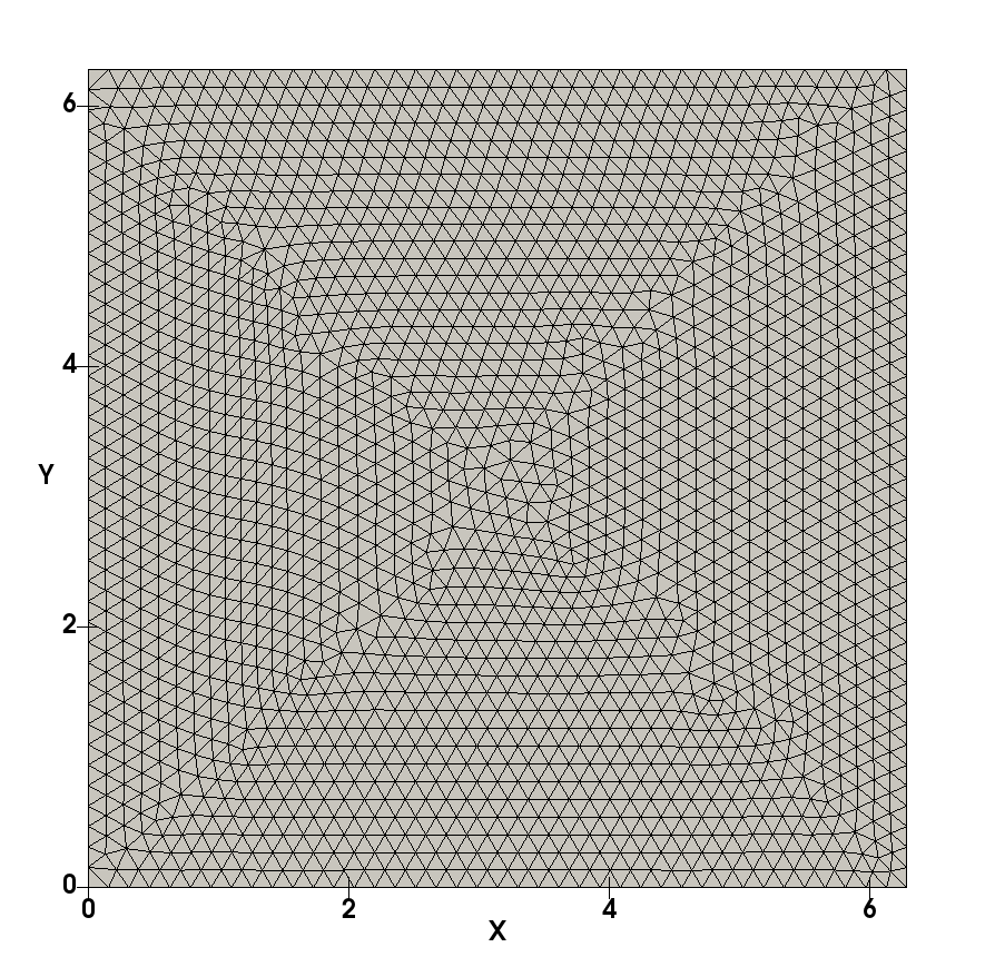
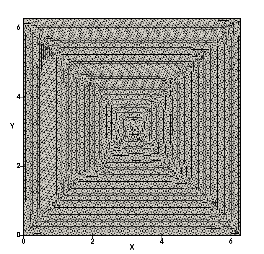
Figure 1. Example 2: the computational mesh. Left: coarse mesh. Right: fine mesh.

Contours of the vorticity $\omega_{h}:=\nabla_{h}\times\boldsymbol{u}_{h}$ at $t=1$ and $t=2$ are shown in Fig. 2. It is clear to observe the vorticity resolution improvement from the coarse mesh to the fine mesh at time $t=2$, where sharp unresolved layers have been developed.

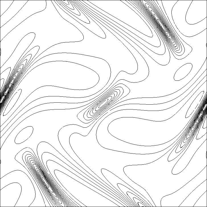
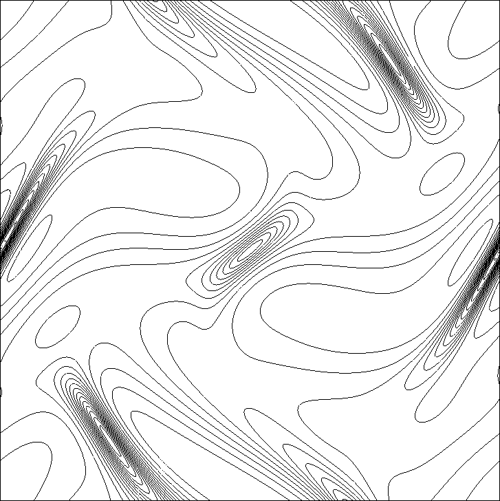
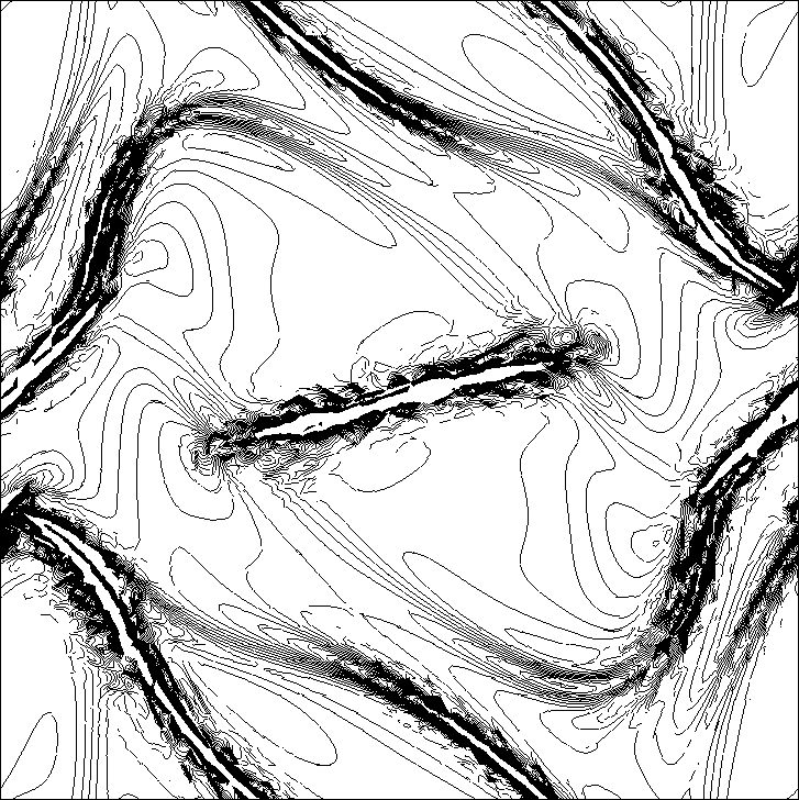
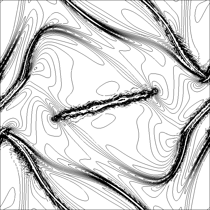
Figure 2. Example 2: Contour of vorticity. 30 equally spaced contour lines between $-15$ and $15$. Left: results on the coarse mesh; right: results on the fine mesh. Top: $t=1$; bottom: $t=2$. $P^{3}$ approximation.

We then plot the time history of kinetic energy $(\boldsymbol{u}_{h},\boldsymbol{u}_{h})_{\mathcal{T}_{h}}$, magnetic energy $(\boldsymbol{B}_{h},\boldsymbol{B}_{h})_{\mathcal{T}_{h}}$, and the total energy (kinetic+magnetic) in Fig. 3. We observe an energy transformation from kinetic energy to magnetic energy. We also observe that the total energy is monotonically decreasing, which is to be expected since both our spatial and temporal discretization are dissipative. The dissipated energy at time $t=2$ for the scheme on the coarse mesh is about $5\%$, while that on the fine mesh is about $2.5\%$.

Figure 3. Example 2: the time history of kinetic, magnetic, and total energy.

Example 3: MHD Kevin-Helmholtz instability problem

We consider an incompressible MHD Kevin-Helmholtz instability problem, the set-up is adapted from [Frank96] where a compressible MHD Kevin-Helmholtz instability problem was studied. The inviscid equations (1) on the domain $[0,L]\times[0,L]$ with $L=1$ is solved with a periodic boundary condition on the $x$-direction, and the slip wall boundary condition for both the velocity and magnetic field $\boldsymbol{u}\cdot\boldsymbol{n}=\boldsymbol{B}\cdot\boldsymbol{n}=0$ in the $y$-direction. The initial conditions are taken to be

$$u_{1}(x,y,0)= \;-\frac{u_{0}}{2}\,\mathrm{tanh}\left(\frac{y-L/2}{a}\right)+c_{n}\partial_{y}\psi(x,y),$$

$$u_{2}(x,y,0)= \;-c_{n}\partial_{x}\psi(x,y),$$

$$B_{1}(x,y,0)= \;\frac{u_{0}}{M_{A}},$$

$$B_{2}(x,y,0)= \;0,$$

with corresponding stream function

$$\psi(x,y)=u_{0}\exp\left(-\frac{(y-L/2)^{2}}{a^{2}}\right)\cos\left(\frac{2\pi}{L}x\right).$$

Here, $a=L/20=0.05$ is the velocity shear scale length, $c_{n}=10^{-3}$ is the noise scaling factor, and $M_{A}$ is the Alfvénic Mach number. Similar as in [Frank96], we take $M_{A}=2.5$ (strong magnetic field) and $M_{A}=5$ (weak magnetic field) in our numerical simulation. For comparison purpose, we also present numerical results for the hydrodynamic case (corresponding to $M_{A}=+\infty$). Introducing the scaled time $\bar{t}=t/\Gamma$, with $\Gamma=0.106{u_{0}}/{2a}=1.06$, we run the simulation till scaled time $\bar{t}=6$ (corresponding to physical time $t=6.36$).

For all the numerical tests in this example, we consider a uniform rectangular mesh with $256\times 256$ cells. The divergence-free finite element space (2) on rectangular meshes is modified to be

$$\boldsymbol{V}_{\!h}^{k,-1}:= \;\{\boldsymbol{v}\in\Pi_{T\in{\mathcal{T}_{h}}}\mathbf{RT}_{k}(T),\;\;[\![\boldsymbol{v}_{T}\cdot\boldsymbol{n}]\!]_{F}=0\;\;\forall F\in\mathcal{F}_{h},\quad{\nabla\cdot}\boldsymbol{v}=0\text{ on }{\mathcal{T}_{h}}\},$$

where $\mathbf{RT}_{k}(T):=[P_{k+1,k}(T),P_{k,k+1}(T)]$ is the usual Raviart-Thomas [RaviartThomas77] space on a rectangle $T$ with $P_{m,n}(T)$ the space of polynomials with degree at most $m$ in the $x$-direction and at most $n$ in the $y$-direction. We use $k=1$ and $k=2$ for the MHD simulations with $M_{A}=2.5$ and $M_{A}=5$, and use $k=3$ for the hydrodynamic simulation ($M_{A}=+\infty$).

Contour of vorticity $\omega_{h}:=\nabla_{h}\times\boldsymbol{u}_{h}$ for the cases $M_{A}=2.5$, $M_{A}=5$, and $M_{A}=+\infty$ are shown in Fig. 4–6, respectively. Comparing with results for the hydrodynamic case in Fig. 6, we observe that in the strong magnetic field case (Fig. 4), the vortex formation is completely suppressed. However, in the weak magnetic field case (Fig. 5), the vortex is initially been developed (left of Fig. 5), then destroyed (due to locally strong magnetic field), which, in turn, produces a sequence of intermediate vortices. The flow is significantly more complex for the weak magnetic field case in Fig. 5 than that for the strong magnetic field case in Fig.4. These observations are qualitatively in agreement with those in [Frank96] for the compressible MHD simulations. Moreover, it is clear to observe from Fig. 4 and Fig. 5 the resolution improvement from the second order $\mathbf{RT}_{1}$ scheme to the third order $\mathbf{RT}_{2}$ scheme.

Then, in Fig. 7 and Fig. LABEL:fig:kh-e2, we plot the time evolution of kinetic, magnetic, and total energy for the case with $M_{A}=2.5$ and $M_{A}=5$, respectively. Looking at the evolution of the total energy, we observe less numerical dissipation for the third order $\mathbf{RT}_{2}$ scheme over the second order $\mathbf{RT}_{1}$ scheme, just as expected. We also observe from Fig. 7 that there is no significant energy transformation between kinetic and magnetic energy for the strong magnetic field case $M_{A}=2.5$. On the other hand, we see from Fig. LABEL:fig:kh-e2 that the energy transformation for the weak magnetic field case $M_{A}=5$ is quite more complex. In particular, the kinetic energy evolves through four phases: it stays at around the same level till scaled time $\bar{t}\approx 2$, then decays till scaled time $\bar{t}\approx 5$, then increases till scaled time $\bar{t}\approx 5.5$, and then decays till the final scaled time $\bar{t}=6$.

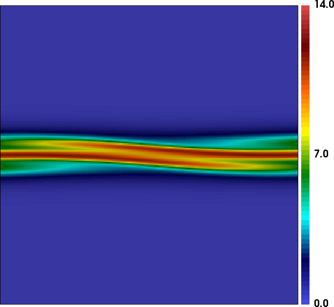
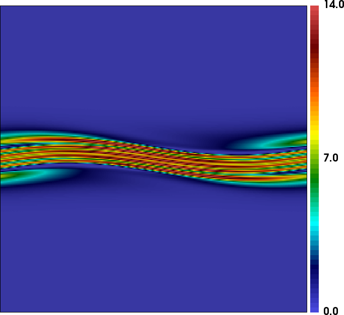
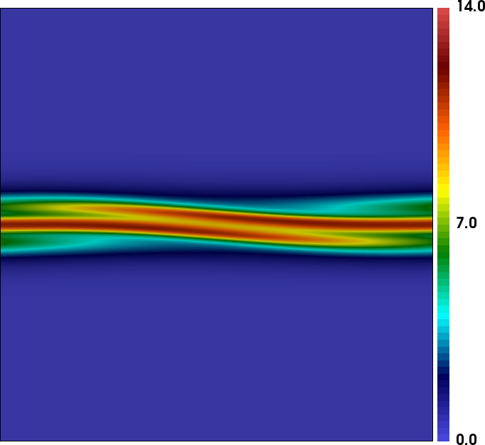
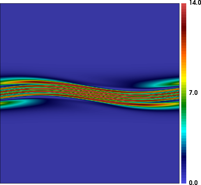
Figure 4. Example 3: Contour of vorticity $\omega_{h}:=\nabla_{h}\times\boldsymbol{u}_{h}$ for the test with $M_{A}=2.5$. Left: $\bar{t}=3$, right: $\bar{t}=6$. Top: $\mathbf{RT}_{1}$ scheme, Bottom: $\mathbf{RT}_{2}$ scheme. Grid size: $256\times 256$.

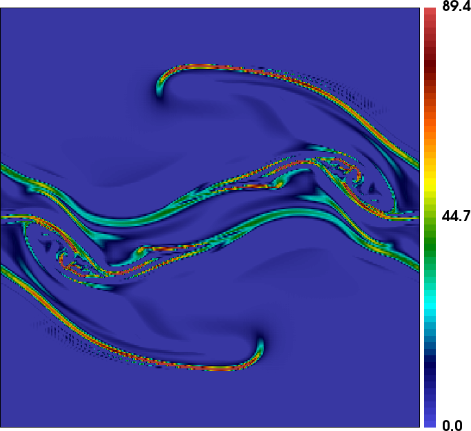
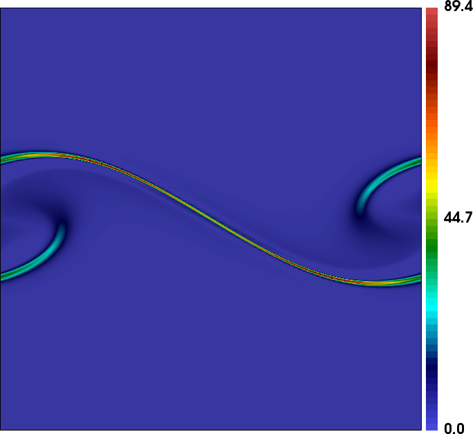
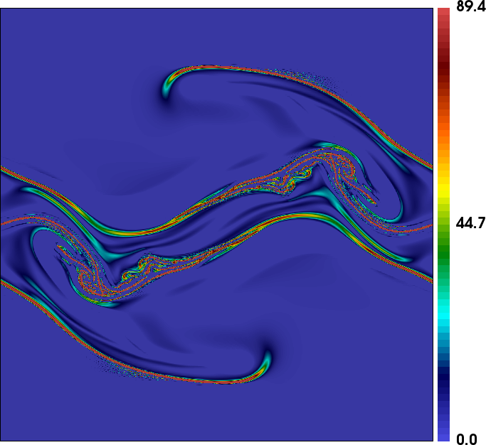
Figure 5. Example 3: Contour of vorticity $\omega_{h}:=\nabla_{h}\times\boldsymbol{u}_{h}$ for the test with $M_{A}=5$. Left: $\bar{t}=3$, right: $\bar{t}=6$. Top: $\mathbf{RT}_{1}$ scheme, Bottom: $\mathbf{RT}_{2}$ scheme. Grid size: $256\times 256$.

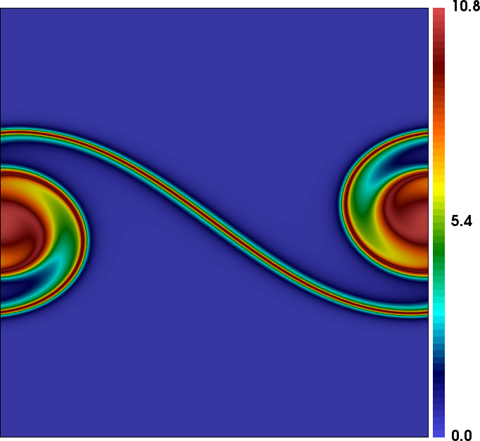
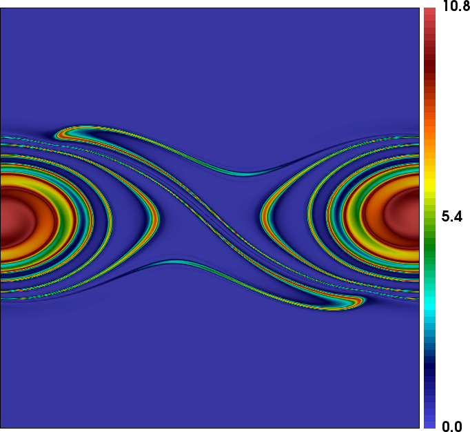
Figure 6. Example 3: Contour of vorticity $\omega_{h}:=\nabla_{h}\times\boldsymbol{u}_{h}$ for the test with $M_{A}=+\infty$ (pure hydrodynamical simulation). $\mathbf{RT}_{3}$ scheme. Grid size: $256\times 256$.

Figure 7. Example 3: the time history of kinetic, magnetic, and total energy for the test with $M_{A}=2.5$.