Independent Low-Rank Matrix Analysis Based on Time-Variant Sub-Gaussian Source Model

Abstract

Independent low-rank matrix analysis (ILRMA) is a fast and stable method for blind audio source separation. Conventional ILRMAs assume time-variant (super-)Gaussian source models, which can only represent signals that follow a super-Gaussian distribution. In this paper, we focus on ILRMA based on a generalized Gaussian distribution (GGD-ILRMA) and propose a new type of GGD-ILRMA that adopts a time-variant sub-Gaussian distribution for the source model. By using a new update scheme called generalized iterative projection for homogeneous source models, we obtain a convergence-guaranteed update rule for demixing spatial parameters. In the experimental evaluation, we show the versatility of the proposed method, i.e., the proposed time-variant sub-Gaussian source model can be applied to various types of source signal.

1 Introduction

Blind source separation (BSS) [1, 2, 3, 4, 5, 6, 7, 8] is a technique for extracting specific sources from an observed multichannel mixture signal without knowing a priori information about the mixing system. The most commonly used algorithm for BSS in the (over)determined case ($\text{number of microphones}\geq\text{number of sources}$) is independent component analysis (ICA) [1]. As a state-of-the-art ICA-based BSS method, Kitamura et al. proposed independent low-rank matrix analysis (ILRMA) [9, 10], which is a unification of independent vector analysis (IVA) [5, 6] and nonnegative matrix factorization (NMF) [11]. ILRMA assumes both statistical independence between sources and a low-rank time-frequency structure for each source, and the frequency-wise demixing systems are estimated without encountering the permutation problem [3, 4]. ILRMA is a faster and more stable algorithm than multichannel NMF (MNMF) [12, 13, 14], which is an algorithm for BSS that estimates the mixing system on the basis of spatial covariance matrices.

The original ILRMA based on Itakura–Saito (IS) divergence assumes a time-variant isotropic complex Gaussian distribution for the source generative model. Hereafter, we refer to the original ILRMA as IS-ILRMA. Recently, various types of source generative model have been proposed in ILRMA for robust BSS. In particular, $t$-ILRMA [15] and GGD-ILRMA [16, 17] have been proposed as generalizations of IS-ILRMA with a complex Student’s $t$ distribution and a complex generalized Gaussian distribution (GGD), respectively. In $t$-ILRMA and GGD-ILRMA, the kurtosis of the generative models’ distributions can be parametrically changed along with the degree-of-freedom parameter in Student’s $t$ distribution and the shape parameter in the GGD. By changing the kurtosis of the distributions, we can control how often the source signal outputs outliers or its expected sparsity. In particular, in sub-Gaussian models, i.e., models that follow distributions with a platykurtic shape, the source signal rarely outputs outliers. Therefore, the sub-Gaussian modeling of sources is expected to accurately estimate the source spectrogram without ignoring its important spectral peaks. Furthermore, many audio sources follow platykurtic distributions; it is known that musical instrument signals obey sub-Gaussian distributions [18].

However, neither conventional $t$-ILRMA nor GGD-ILRMA assumes that the source model follows a sub-Gaussian distribution. Both $t$-ILRMA and GGD-ILRMA can adopt only a super-Gaussian (or Gaussian) model, i.e., models that follow distributions with a leptokurtic shape, for the source model. In $t$-ILRMA, this is because the complex Student’s $t$ distribution becomes only super-Gaussian for any degree-of-freedom parameter. In GGD-ILRMA, on the other hand, it is because the estimation algorithm for the demixing matrix has not yet been derived for a sub-Gaussian case, although the GGD itself can represent a sub-Gaussian distribution depending on its shape parameter. More specifically, the conventional iterative projection (IP) [7], which is an algorithm that updates the demixing matrix mainly used in IVA and ILRMA, cannot be applied to sub-Gaussian-based GGD-ILRMA owing to mathematical difficulties.

In this paper, we propose a new type of ILRMA that assumes time-variant sub-Gaussian source models. This paper includes three novelties. First, we construct a new update scheme for the demixing matrix called generalized IP for homogeneous source models (GIP-HSM). Second, we derive a convergence-guaranteed update rule for the demixing matrix in GGD-ILRMA with a shape parameter of four. To the best of our knowledge, this is the world’s first attempt to model the source signal with a time-variant sub-Gaussian distribution, and we derive the update rule by applying the above-mentioned scheme. Third, we show the validity of the proposed sub-Gaussian GGD-ILRMA via BSS experiments on music and speech signals. We confirm that the proposed method is a versatile approach to source modeling, i.e., the proposed time-variant sub-Gaussian model can represent super-Gaussian or Gaussian signals as well as sub-Gaussian signals owing to its time-variant nature, whereas the conventional models can only represent super-Gaussian or Gaussian signals.

2 Problem Formulation

2.1 Formulation of Demixing Model

Let $N$ and $M$ be the numbers of sources and channels, respectively. The short-time Fourier transforms (STFTs) of the multichannel source, observed, and estimated signals are defined as

$$\bm{s}_{ij} =(s_{ij1},\ldots,s_{ijN})^{\top}\in\mathbb{C}^{N},$$ (1)

$$\bm{x}_{ij} =(x_{ij1},\ldots,x_{ijM})^{\top}\in\mathbb{C}^{M},$$ (2)

$$\bm{y}_{ij} =(y_{ij1},\ldots,y_{ijN})^{\top}\in\mathbb{C}^{N},$$ (3)

where $i=1,\ldots,I$; $j=1,\ldots,J$; $n=1,\ldots,N$; and $m=1\ldots,M$ are the integral indices of the frequency bins, time frames, sources, and channels, respectively, and ^⊤ denotes the transpose. We assume the mixing system

$$\bm{x}_{ij}=\bm{A}_{i}\bm{s}_{ij},$$ (4)

where $\bm{A}_{i}=(\bm{a}_{i1},\ldots,\bm{a}_{iN})\in\mathbb{C}^{M\times N}$ is a frequency-wise mixing matrix and $\bm{a}_{in}$ is the steering vector for the $n$th source. When $M=N$ and $\bm{A}_{i}$ is not a singular matrix, the estimated signal $\bm{y}_{ij}$ can be expressed as

$$\bm{y}_{ij}=\bm{W}_{i}\bm{x}_{ij},$$ (5)

where $\bm{W}_{i}=\bm{A}_{i}^{-1}=(\bm{w}_{i1},\ldots,\bm{w}_{iN})^{\mathsf{H}}$ is the demixing matrix, $\bm{w}_{in}$ is the demixing filter for the $n$th source, and ^H denotes the Hermitian transpose. ILRMA estimates both $\bm{W}_{i}$ and $\bm{y}_{ij}$ from only the observation $\bm{x}_{ij}$ assuming statistical independence between $s_{ijn}$ and $s_{ijn^{\prime}}$, where $n\neq n^{\prime}$.

2.2 Generative Model and Cost Function in GGD-ILRMA

GGD-ILRMA utilizes the isotropic complex GGD. The probability density function of the GGD is

$$p(z)=\dfrac{\beta}{2\pi r^{2}\Gamma(2/\beta)}\exp\biggl{(}-{\dfrac{\left\lvert z\right\rvert^{\beta}}{r^{\beta}}}\biggr{)},$$ (6)

where $\beta$ is the shape parameter, $r$ is the scale parameter, and $\Gamma(\cdot)$ is the gamma function. Fig. 1 shows the shapes of the GGD with $\beta=2$ and $\beta=4$. When $\beta=2$, (6) corresponds to the probability density function of the complex Gaussian distribution with a mesokurtic shape. In the case of $0<\beta<2$, the distribution becomes super-Gaussian with a leptokurtic shape. In the case of $\beta>2$, the distribution becomes sub-Gaussian with a platykurtic shape.

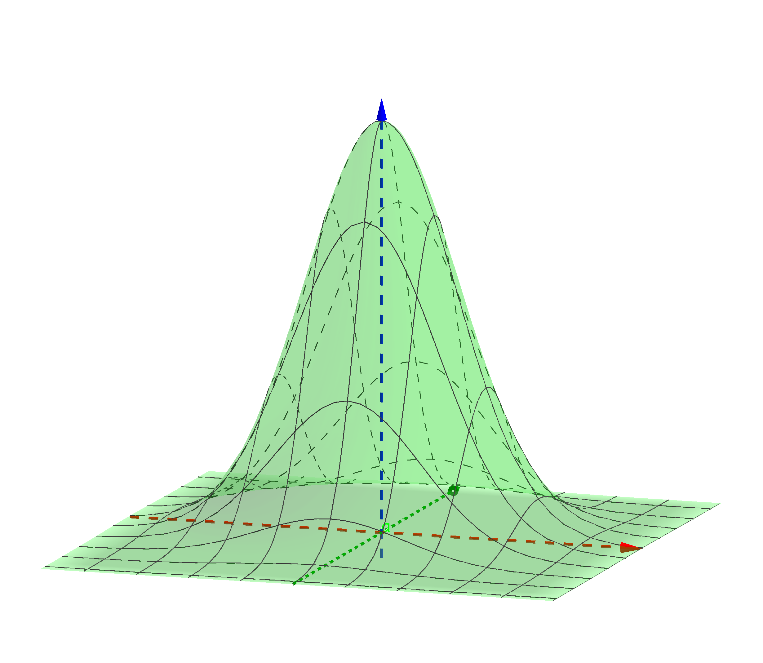
(a) GGD with $\beta=2$.

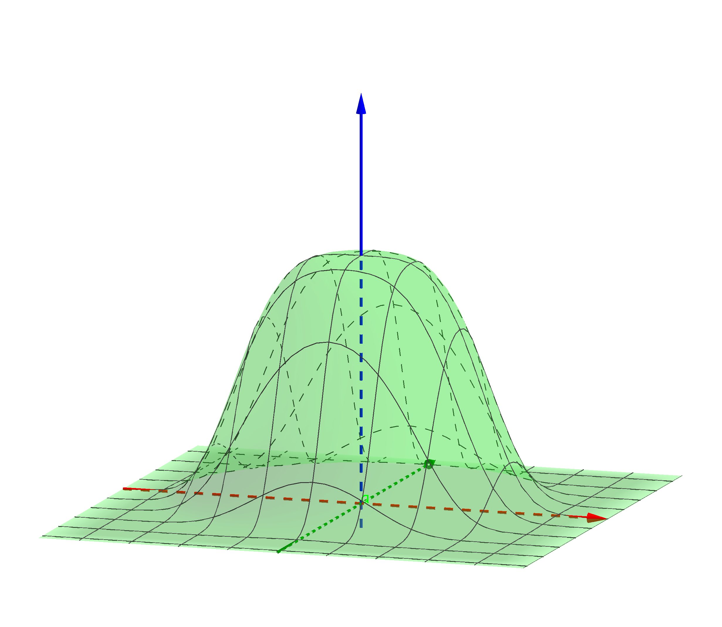
(b) GGD with $\beta=4$.

Figure 1: Examples of shapes of complex GGD. (a) When $\beta=2$, shape of GGD corresponds to that of Gaussian distribution. (b) When $\beta=4$, GGD is platykurtic.

In GGD-ILRMA, we assume the time-variant isotropic complex GGD as the source generative model, which is independently defined in each time-frequency slot as follows:

$$p(\bm{Y}_{n}) =\prod_{i,j}p(y_{ijn})$$

$$=\prod_{i,j}\dfrac{\beta}{2\pi{r_{ijn}}^{2}\Gamma(2/\beta)}\exp\biggl{(}-{\dfrac{\left\lvert y_{ijn}\right\rvert^{\beta}}{{r_{ijn}}^{\beta}}}\biggr{)},$$ (7)

$${r_{ijn}}^{p} =\sum_{k}t_{ikn}v_{kjn},$$ (8)

where the local distribution $p(y_{ijn})$ is defined as a circularly symmetric complex Gaussian distribution, i.e., the probability of $p(y_{ijn})$ only depends on the power of the complex value $y_{ijn}$. $r_{ijn}$ is the time-frequency-varying scale parameter and $p$ is the domain parameter in NMF modeling. Moreover, the variables $t_{ikn}$ and $v_{kjn}$ are the elements of the basis matrix $\bm{T}_{n}\in\mathbb{R}_{\geq 0}^{I\times K}$ and the activation matrix $\bm{V}_{n}\in\mathbb{R}_{\geq 0}^{K\times J}$, respectively, where $\mathbb{R}_{\geq 0}$ denotes the set of nonnegative real numbers. $k=1,\cdots,K$ is the integral index, and $K$ is set to a much smaller value than $I$ and $J$, which leads to the low-rank approximation. From (7), the negative log-likelihood function $\mathcal{L}_{\mathrm{GGD}}$ of the observed signal $\bm{x}_{ij}$ can be obtained as follows by assuming independence between sources:

$$\mathcal{L}_{\mathrm{GGD}} =-2J\sum_{i}\log\left\lvert\det\bm{W}_{i}\right\rvert$$

$$\phantom{{}={}}+\sum_{i,j,n}\left(\dfrac{\left\lvert y_{ijn}\right\rvert^{\beta}}{{r_{ijn}}^{\beta}}+2\log r_{ijn}\right),$$ (9)

where $y_{ijn}=\bm{w}_{in}\bm{x}_{ij}$ and we used the transformation of random variables from $\bm{x}_{ij}$ to $\bm{y}_{ij}$. The cost function of GGD-ILRMA (9) coincides with that of IS-ILRMA when $\beta=p=2$. By minimizing (9) w.r.t. $\bm{W}_{i}$ and $r_{ijn}$ under the limitation (8), we estimate the demixing system that maximizes the independence between sources.

Fig. 2 shows a conceptual model of GGD-ILRMA. When each of the original sources has a low-rank spectrogram, the spectrogram of their mixture should be more complicated, where the rank of the mixture spectrogram will be greater than that of the source spectrogram. On the basis of this assumption, in GGD-ILRMA, the low-rank constraint for each estimated spectrogram is introduced by employing NMF. The demixing matrix $\bm{W}_{i}$ is estimated so that the spectrogram of the estimated signal becomes a low-rank matrix modeled by $\bm{T}_{n}\bm{V}_{n}$, whose rank is at most $K$. The estimation of $\bm{W}_{i},\bm{T}_{n}$, and $\bm{V}_{n}$ can consistently be carried out by minimizing (9) in a fully blind manner.

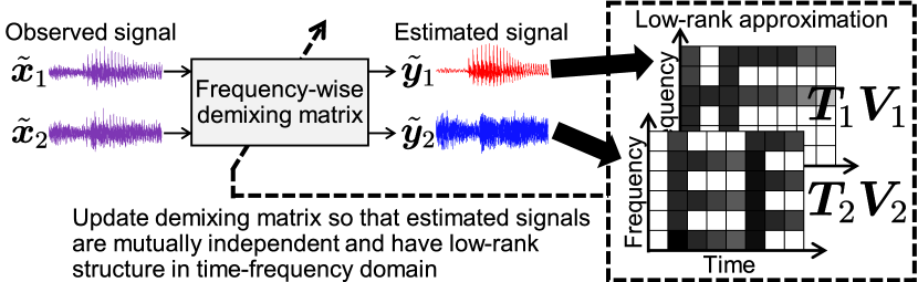
Figure 2: Principle of source separation in GGD-ILRMA, where $\tilde{\bm{x}}_{m}$ and $\tilde{\bm{y}}_{n}$ are time-domain signals of $x_{ijn}$ and $y_{ijn}$, respectively.

3 Conventional Method

3.1 Update Rule for Demixing Matrix

In IS-ILRMA, the demixing matrix $\bm{W}_{i}$ can be efficiently updated by IP, which can be applied only when the cost function is the sum of $-\log\left\lvert\det\bm{W}_{i}\right\rvert$ and the quadratic form of $\bm{w}_{in}$ (this corresponds to GGD-ILRMA with $\beta=2$). In GGD-ILRMA, the update rule of $\bm{W}_{i}$ is also derived using the majorization-minimization (MM) algorithm [19]. When $0<\beta\leq 2$, we can use the following inequality of weighted arithmetic and geometric means to design the majorization function:

$$\left\lvert y_{ijn}\right\rvert^{\beta}\leq\dfrac{\beta}{2}\dfrac{\left\lvert y_{ijn}\right\rvert^{2}}{{\alpha_{ijn}}^{2-\beta}}+\left(1-\dfrac{\beta}{2}\right){\alpha_{ijn}}^{\beta},$$ (10)

where $\alpha_{ijn}$ is an auxiliary variable and the equality of (10) holds if and only if $\alpha_{ijn}=\left\lvert y_{ijn}\right\rvert$. By applying (10) to (9), the majorization function of (9) can be designed as

$$\mathcal{L}_{\mathrm{GGD}} \leq-2J\sum_{i}\log\left\lvert\det\bm{W}_{i}\right\rvert$$

$$\phantom{{}={}}+J\sum_{i,n}\bm{w}_{in}^{\mathsf{H}}\bm{F}_{in}\bm{w}_{in}+\mathrm{const.},$$ (11)

$$\bm{F}_{in} =\dfrac{\beta}{2J}\sum_{j}\dfrac{1}{{\alpha_{ijn}}^{2-\beta}(\sum_{k}t_{ikn}v_{kjn})^{\frac{\beta}{p}}}\bm{x}_{ij}\bm{x}_{ij}^{\mathsf{H}},$$ (12)

where the constant term is independent of $\bm{w}_{in}$. By applying IP to (11) and substituting the equality condition $\alpha_{ijn}=\left\lvert y_{ijn}\right\rvert$ into (12), the update rule for $\bm{W}_{i}$ is derived as

$$\bm{F}_{in} =\dfrac{\beta}{2J}\sum_{j}\dfrac{1}{\left\lvert y_{ijn}\right\rvert^{2-\beta}(\sum_{k}t_{ikn}v_{kjn})^{\frac{\beta}{p}}}\bm{x}_{ij}\bm{x}_{ij}^{\mathsf{H}},$$ (13)

$$\bm{w}_{in} \leftarrow\bm{F}_{in}^{-1}\bm{W}_{i}^{-1}\bm{e}_{n},$$ (14)

$$\bm{w}_{in} \leftarrow\bm{w}_{in}\sqrt{1/(\bm{w}_{in}^{\mathsf{H}}\bm{F}_{in}\bm{w}_{in})}.$$ (15)

When $\beta=p=2$, these update rules (13)–(15) coincide with those in IS-ILRMA.

Note that the update rules (13)–(15) are valid only when $0<\beta\leq 2$, which is equivalent to the condition that the inequality (10) holds. In fact, when $\beta>2$, it is thought to be impossible to design a majorization function to which we can apply IP because no quadratic function w.r.t. $x$ can majorize $x^{\beta}$.

Conventional GGD-ILRMA achieves various types of source generative model: when $\beta=2$, the entry of the source spectrogram follows the complex Gaussian distribution (the same model as that of IS-ILRMA), and when $\beta<2$, the entry of the source spectrogram follows the complex leptokurtic distribution. However, a source generative model that follows a platykurtic complex GGD is yet to be achieved. Since the marginal distribution of the time-variant super-Gaussian or Gaussian model w.r.t. the time frame becomes only super-Gaussian, any signals that follow sub-Gaussian distributions, such as music signals, cannot be appropriately dealt with by the conventional GGD-ILRMA.

3.2 Update Rule for Low-Rank Source Model

The update rules for $\bm{T}_{n}$ and $\bm{V}_{n}$ in IS-ILRMA and GGD-ILRMA can be derived by the MM algorithm, which is a popular approach for NMF. We obtain the following update rules:

$$t_{ikn} \leftarrow t_{ikn}\left(\dfrac{\beta\sum_{j}\dfrac{\left\lvert y_{ijn}\right\rvert^{\beta}}{(\sum_{k^{\prime}}t_{ik^{\prime}n}v_{k^{\prime}jn})^{\frac{\beta}{p}+1}}v_{kjn}}{2\sum_{j}\dfrac{1}{\sum_{k^{\prime}}t_{ik^{\prime}n}v_{k^{\prime}jn}}v_{kjn}}\right)^{\frac{p}{\beta+p}},$$ (16)

$$v_{kjn} \leftarrow v_{kjn}\left(\dfrac{\beta\sum_{j}\dfrac{\left\lvert y_{ijn}\right\rvert^{\beta}}{(\sum_{k^{\prime}}t_{ik^{\prime}n}v_{k^{\prime}jn})^{\frac{\beta}{p}+1}}t_{ikn}}{2\sum_{j}\dfrac{1}{\sum_{k^{\prime}}t_{ik^{\prime}n}v_{k^{\prime}jn}}t_{ikn}}\right)^{\frac{p}{\beta+p}}.$$ (17)

See Appendix .1 for their detailed derivation.

In GGD-ILRMA, the cost function (9) is minimized by alternately repeating the update of the demixing matrix $\bm{W}_{i}$ using (13)–(15) and the update of the low-rank source models $\bm{T}_{n}$ and $\bm{V}_{n}$ using (16) and (17), respectively. A monotonic decrease in the cost is guaranteed over these update rules.

4 Proposed Method

4.1 Motivation

The conventional methods [9, 16] have a limitation that the source signal cannot be appropriately represented when the signal follows a sub-Gaussian distribution. In this paper, we propose an MM-algorithm-based update rule for GGD-ILRMA to maximize the likelihood based on the sub-Gaussian source model. To derive the update rule, we also extend the problem of demixing matrix estimation into a more generalized form and propose its optimization scheme based on GIP-HSM.

In contrast to the time-variant super-Gaussian or Gaussian model, the marginal distribution of the time-variant sub-Gaussian model w.r.t. the time frame can be sub-Gaussian as well as Gaussian or super-Gaussian, depending on its time variance of the scale parameter $r_{ijn}$. For example, the time-variant sub-Gaussian model is platykurtic when $r_{ijn}$ is constant w.r.t. the time frame, whereas it becomes mesokurtic or leptokurtic when $r_{ijn}$ fluctuates appropriately. This shows that the proposed time-variant sub-Gaussian model covers distributions with a wider range between platykurtic and leptokurtic shapes than other conventional source models. Therefore, the proposed GGD-ILRMA is expected to have a robust performance against the variation of the target signals.

4.2 Derivation of GIP-HSM

The cost functions of IS-ILRMA and GGD-ILRMA are generalized as

$$\mathcal{L} =\sum_{i=1}^{I}\left[-2\log\left\lvert\det\bm{W}_{i}\right\rvert+\sum_{n=1}^{N}f_{in}(\bm{w}_{in})\right]+\mathrm{const.},$$ (18)

where the constant term is independent of $\bm{w}_{in}$ and $f_{in}\colon\mathbb{C}^{N}\to\mathbb{R}$ is a real-valued function that satisfies the following three conditions:

1. $f_{in}(\bm{w})$ is differentiable w.r.t. $\bm{w}$ at an arbitrary point.

2. ${}^{\forall}c>0$, $\left\{\bm{w}\in\mathbb{C}^{N}\mathrel{}\middle|\mathrel{}f_{in}(\bm{w})\leq c\right\}$ is convex (naturally satisfied when $f_{in}(\bm{w})$ is convex).

3. ${}^{\forall}\eta$, $f_{in}(\eta\bm{w})=\eta^{d}f_{in}(\bm{w})$, namely, $f_{in}$ is a homogeneous function of degree $d$.

The term $f_{in}(\bm{w}_{in})$ is determined by the distribution of the source generative model, e.g., $f_{in}(\bm{w}_{in})=(1/J)\sum_{j}\left({\lvert\bm{w}_{in}^{\mathsf{H}}\bm{x}_{ij}\rvert^{\beta}}/{{r_{ijn}}^{\beta}}\right)$ in GGD-ILRMA.

Here we show that the optimization of (18) w.r.t. $\bm{w}_{in}$ is composed of “direction optimization” and “scale optimization” for each frequency bin. Let $\bm{u}_{in}$ be an $N$-dimensional vector that satisfies $f_{in}(\bm{u}_{in})=1$. Then, $\bm{w}_{in}$ can be uniquely represented as $\bm{w}_{in}=\eta_{in}\bm{u}_{in}$, where $\eta_{in}$ is a positive real value. By regarding $f_{in}(\bm{u})$ as the norm of $\bm{u}$, we can interpret $\bm{u}_{in}$ as a unit vector w.r.t. the $f_{in}$-norm. Substituting $\bm{w}_{in}=\eta_{in}\bm{u}_{in}$ into (18), the cost function is represented as

$$\mathcal{L} =\sum_{i=1}^{I}\biggl{[}-2\log\left\lvert\det\begin{bmatrix}\,\eta_{1}\bm{u}_{1}&\cdots&\eta_{N}\bm{u}_{N}\mbox{\,}\end{bmatrix}^{\mathsf{H}}\right\rvert$$

$$\hphantom{{}=\sum_{i=1}^{N}[]}+\sum_{n=1}^{N}f_{in}(\eta_{in}\bm{u}_{in})\biggr{]}$$

$$=\sum_{i=1}^{I}\left[-2\log\left(\prod_{n}{\eta_{in}}\cdot\left\lvert\det\bm{U}_{i}\right\rvert\right)+\sum_{n=1}^{N}{\eta_{in}}^{d}f_{in}(\bm{u}_{in})\right]$$

$$=\sum_{i=1}^{I}\left[-2\log\left\lvert\det\bm{U}_{i}\right\rvert+\sum_{n=1}^{N}\left[-2\log{\eta_{in}}+{\eta_{in}}^{d}\right]\right],$$ (19)

where $\bm{U}_{i}=\begin{bmatrix}\,\bm{u}_{i1}&\cdots&\bm{u}_{iN}\mbox{\,}\end{bmatrix}^{\mathsf{H}}$. Therefore, the minimization of the cost function can be interpreted as the minimization of $-\log\left\lvert\det\bm{U}_{i}\right\rvert$ for each frequency bin and the minimization of $-2\log\eta_{in}+{\eta_{in}}^{d}$ for each source and frequency bin. These direction optimization and scale optimization problems are independent of each other. The optimal $\eta_{in}$ can be calculated by a closed form because the derivative of the cost function w.r.t. $\eta_{in}$ can be written as

$$\dfrac{d}{d\eta_{in}}(-2\log\eta_{in}+{\eta_{in}}^{d})=-\dfrac{2}{\eta_{in}}+d{\eta_{in}}^{d-1}.$$ (20)

Hence, letting the right side of (20) be zero, we can obtain the optimal $\eta_{in}$ as

$$\eta_{in}=\sqrt[d]{2/d}.$$ (21)

The actual difficulty in the optimization of the demixing matrix is the direction optimization, i.e., the minimization of $-2\log\left\lvert\det\bm{U}_{i}\right\rvert$. Since minimizing $-\log x^{2}$ is equivalent to maximizing $x^{2}$, we can reformulate this problem as

$$\text{maximize\ }{\left\lvert\det\bm{U}_{i}\right\rvert^{2}}\quad\text{s.t.\ }f_{in}(\bm{u}_{in})=1.$$ (22)

Since it is generally difficult to solve this problem by a closed form, we apply an approach called vectorwise coordinate descent. In this algorithm, we focus on $\bm{u}_{in}$, namely, the Hermitian transpose of a particular row vector of $\bm{U}_{i}$. By cofactor expansion, we can deform the problem (22) as

$$\text{maximize\ }{\left\lvert\bm{b}_{in}^{\mathsf{H}}\bm{u}_{in}\right\rvert^{2}}\quad\text{s.t.\ }f_{in}(\bm{u}_{in})=1,$$ (23)

where $\bm{b}_{in}$ is a column vector of the adjugate matrix $\bm{B}_{i}=\begin{bmatrix}\,\bm{b}_{i1}&\cdots&\bm{b}_{iN}\mbox{\,}\end{bmatrix}^{\mathsf{H}}$ of $\bm{U}_{i}$. Since $\bm{b}_{in}$ only depends on $\bm{u}_{in^{\prime}}\,(n^{\prime}\neq n)$ and is independent of $\bm{u}_{in}$, (23) can be regarded as a function of $\bm{u}_{in}$ by fixing the other row vectors of $\bm{U}_{i}$. Using the method of Lagrange multipliers, the stationary condition is

$$\bm{b}_{in}(\bm{b}_{in}^{\mathsf{H}}\bm{u}_{in})+\lambda\dfrac{\partial f_{in}}{\partial\bm{u}_{in}^{\mathsf{H}}}(\bm{u}_{in})=0,$$ (24)

where $\lambda$ is a Lagrange multiplier. Since $(\bm{b}_{in}^{\mathsf{H}}\bm{u}_{in})$ is a scalar, the stationary condition can be rewritten as

$$\dfrac{\partial f_{in}}{\partial\bm{u}_{in}^{\mathsf{H}}}(\bm{u}_{in})\parallel\bm{b}_{in},$$ (25)

where the binary relation “$\bm{x}\parallel\bm{y}$” means that $\bm{x}$ is parallel to $\bm{y}$. In (25), $\bm{b}_{in}$ is represented in terms of $\bm{W}_{in}$ as

$$\bm{b}_{in} =(\det\bm{U}_{i})\bm{U}_{i}^{-1}\bm{e}_{n}$$

$$=(\det\bm{U}_{i})(\mathrm{diag}(\eta_{i1}^{-1},\ldots,\eta_{iN}^{-1})\bm{W}_{i})^{-1}\bm{e}_{n}$$

$$=(\det\bm{U}_{i})\bm{W}_{i}^{-1}\mathrm{diag}(\eta_{i1},\ldots,\eta_{iN})\bm{e}_{n}$$

$$=(\eta_{in}\det\bm{U}_{i})\bm{W}_{i}^{-1}\bm{e}_{n}$$

$$\parallel\bm{W}_{i}^{-1}\bm{e}_{n},$$ (26)

where $\mathrm{diag}(c_{1},\ldots,c_{N})$ denotes the $N\times N$ diagonal matrix whose $(n,n)$th element is $c_{n}$, and $\bm{e}_{n}$ is an $N$-dimensional vector whose $n$th element is one and whose other elements are zero. Since $f_{in}$ is convex, the stationary point of the objective function (23) must also be the optimal point. Therefore, the cost function (19) that includes (22) monotonically decreases with each update of the direction $\bm{u}_{in}$.

In conclusion, to minimize the cost function (18), we update the vector $\bm{w}_{in}$ by the following two steps in GIP-HSM. (a) Find a vector $\bm{w}_{in}^{\prime}$ that satisfies

$$\frac{\partial f_{in}}{\partial\bm{w}_{in}^{\mathsf{H}}}(\bm{w}_{in}^{\prime})\parallel\bm{W}_{i}^{-1}\bm{e}_{n}.$$ (27)

(b) Update $\bm{w}_{in}$ as

$$\rule[-0.86108pt]{0.0pt}{9.47217pt}\bm{w}_{in}\leftarrow\bm{w}_{in}^{\prime}\sqrt[d]{2/(d\cdot f_{in}(\bm{w}_{in}^{\prime}))}.$$ (28)

The first step (a) and second step (b) correspond to the direction and scale optimizations, respectively. Note that $\bm{w}_{in}^{\prime}$ calculated in the first step does not need to satisfy $f_{in}(\bm{w}_{in}^{\prime})=1$ because the scale is automatically adjusted in the second step. In fact, if $\bm{w}_{in}^{\prime}$ is represented as $\bm{w}_{in}^{\prime}=\eta_{in}^{\prime}\bm{u}_{in}$, the second step results in

$$\bm{w}_{in}\leftarrow\eta_{in}^{\prime}\bm{u}_{in}\cdot\sqrt[d]{2/(d\cdot{\eta_{in}^{\prime}}^{d})}=\bm{u}_{in}\sqrt[d]{2/d},$$ (29)

at which point both the direction and the scale are optimized.

4.3 Sub-Gaussian ILRMA Based on GIP-HSM

Using GIP-HSM, we propose a new update rule in GGD-ILRMA whose shape parameter $\beta$ is set to four (time-variant sub-Gaussian model). The cost function of GGD-ILRMA with $\beta=4$ is written as

$$\mathcal{J} =-2J\sum_{i}\log\left\lvert\det\bm{W}_{i}\right\rvert+\sum_{i,j,n}{\dfrac{\lvert\bm{w}_{in}^{\mathsf{H}}\bm{x}_{ij}\rvert^{4}}{{r_{ijn}}^{4}}}+\mathrm{const.},$$ (30)

where the constant term is independent of $\bm{w}_{in}$. It seems possible to apply GIP-HSM by letting $f_{in}(\bm{w}_{in})=(1/J)\sum_{j}\left({\lvert\bm{w}_{in}^{\mathsf{H}}\bm{x}_{ij}\rvert^{4}}/{{r_{ijn}}^{4}}\right)$. In this case, however, it is difficult to solve (27), which is reduced to a cubic vector equation w.r.t. $\bm{w}_{in}^{\prime}$. Instead, we apply an MM algorithm to derive an update rule that does not contain any cubic vector equations. Hereafter, we prove the following theorem, and then design a new type of majorization function of (30) using the theorem.

Theorem 1

Let $f(\bm{w})=(1/J)\sum_{j=1}^{J}({\lvert\bm{w}^{\mathsf{H}}\bm{x}_{j}\rvert^{4}}/{{r_{j}}^{4}})$ and $g(\bm{w})=(\bm{w}^{\mathsf{H}}\bm{G}\bm{w})^{2}$, where $\bm{G}$ is defined in terms of a vector $\tilde{\bm{w}}$ as

$$\bm{H} =\begin{bmatrix}\,\frac{1}{r_{1}}\bm{x}_{1}&\cdots&\frac{1}{r_{J}}\bm{x}_{J}\mbox{\,}\end{bmatrix},$$ (31)

$$\tilde{\bm{q}} =\begin{bmatrix}\,\tilde{q}_{1}&\cdots&\tilde{q}_{J}\mbox{\,}\end{bmatrix}^{\top}=\bm{H}^{\mathsf{H}}\tilde{\bm{w}},$$ (32)

$$\tilde{\bm{Q}} =\begin{bmatrix}\left\lVert\tilde{\bm{q}}\right\rVert^{2}&{-\tilde{q}_{1}\tilde{q}_{2}^{*}}&\cdots&{-\tilde{q}_{1}\tilde{q}_{J}^{*}}\\ \rule{0.0pt}{12.91663pt}{-\tilde{q}_{2}\tilde{q}_{1}^{*}}&\left\lVert\tilde{\bm{q}}\right\rVert^{2}&\cdots&{-\tilde{q}_{2}\tilde{q}_{J}^{*}}\\ \vdots&\vdots&\ddots&\vdots\\ \rule{0.0pt}{12.91663pt}{-\tilde{q}_{J}\tilde{q}_{1}^{*}}&{-\tilde{q}_{J}\tilde{q}_{2}^{*}}&\cdots&\left\lVert\tilde{\bm{q}}\right\rVert^{2}\end{bmatrix},$$ (33)

$$\bm{G} =\dfrac{1}{\sqrt{J\sum_{j}\left\lvert\tilde{q}_{j}\right\rvert^{4}}}\bm{H}\tilde{\bm{Q}}\bm{H}^{\mathsf{H}}.$$ (34)

Then, $g(\bm{w})$ satisfies $f(\bm{w})\leq g(\bm{w})$ for arbitrary $\bm{w}$ and the equality holds when $\bm{w}=\tilde{\bm{w}}$.

Proof 4.2.

Let $\bm{q}=\begin{bmatrix}\,q_{1}&\cdots&q_{J}\mbox{\,}\end{bmatrix}^{\top}=\bm{H}^{\mathsf{H}}\bm{w}$. $f(\bm{w})$ and $g(\bm{w})$ can be written as

$$f(\bm{w}) =\dfrac{1}{J}\sum_{j}\left\lvert q_{j}\right\rvert^{4},$$ (35)

$$g(\bm{w}) =\dfrac{1}{{J\sum_{j}\left\lvert\tilde{q}_{j}\right\rvert^{4}}}(\bm{q}^{\mathsf{H}}\tilde{\bm{Q}}\bm{q})^{2}.$$ (36)

Then, the objective inequality $f(\bm{w})\leq g(\bm{w})$ holds if and only if

$$\biggl{(}\sum_{j}\left\lvert q_{j}\right\rvert^{4}\biggr{)}\biggl{(}\sum_{j}\left\lvert\tilde{q}_{j}\right\rvert^{4}\biggr{)}\leq(\bm{q}^{\mathsf{H}}\tilde{\bm{Q}}\bm{q})^{2}.$$ (37)

The quadratic form of the right side in (37) can be deformed as

$$\bm{q}^{\mathsf{H}}\tilde{\bm{Q}}\bm{q} =\mathop{\mathrm{tr}}(\tilde{\bm{Q}}\bm{q}\bm{q}^{\mathsf{H}})$$

$$=\biggl{(}\sum_{j}\left\lvert q_{j}\right\rvert^{2}\biggr{)}\left\lVert\tilde{\bm{q}}\right\rVert-\sum_{i\neq j}q_{i}q_{j}^{*}\tilde{q}_{i}^{*}\tilde{q}_{j}$$

$$=\biggl{(}\sum_{j}\left\lvert q_{j}\right\rvert^{2}\biggr{)}\biggl{(}\sum_{j}\left\lvert\tilde{q}_{j}\right\rvert^{2}\biggr{)}-\sum_{i\neq j}q_{i}q_{j}^{*}\tilde{q}_{i}^{*}\tilde{q}_{j}.$$ (38)

Hence, we prove the following inequality hereafter:

$$\biggl{(}\sum_{j}\left\lvert q_{j}\right\rvert^{4}\biggr{)}\biggl{(}\sum_{j}\left\lvert\tilde{q}_{j}\right\rvert^{4}\biggr{)}$$

$$\leq\left(\biggl{(}\sum_{j}\left\lvert q_{j}\right\rvert^{2}\biggr{)}\biggl{(}\sum_{j}\left\lvert\tilde{q}_{j}\right\rvert^{2}\biggr{)}-\sum_{i\neq j}q_{i}q_{j}^{*}\tilde{q}_{i}^{*}\tilde{q}_{j}\right)^{2}.$$ (39)

Let

$$x_{1} =\sum_{j}\left\lvert q_{j}\right\rvert^{2},$$ (40)

$$x_{2} =\sqrt{\sum_{i\neq j}\left\lvert q_{i}\right\rvert^{2}\left\lvert q_{j}\right\rvert^{2}},$$ (41)

$$y_{1} =\sum_{j}\left\lvert\tilde{q}_{j}\right\rvert^{2},$$ (42)

$$y_{2} =\sqrt{\sum_{i\neq j}\left\lvert\tilde{q}_{i}\right\rvert^{2}\left\lvert\tilde{q}_{j}\right\rvert^{2}}.$$ (43)

Since

$${x_{1}}^{2}-{x_{2}}^{2}=\sum_{j}\left\lvert q_{j}\right\rvert^{4}\geq 0,$$ (44)

$${y_{1}}^{2}-{y_{2}}^{2}=\sum_{j}\left\lvert\tilde{q}_{j}\right\rvert^{4}\geq 0,$$ (45)

and $x_{1},x_{2},y_{1},y_{2}\geq 0$, it is obvious that

$$x_{1}y_{1}-x_{2}y_{2}\geq 0.$$ (46)

Furthermore, we obtain the following inequality by applying the Cauchy–Schwarz inequality:

$$x_{2}y_{2} =\sqrt{\biggl{(}\sum_{i\neq j}\left\lvert q_{i}\right\rvert^{2}\left\lvert q_{j}\right\rvert^{2}\biggr{)}\biggl{(}\sum_{i\neq j}\left\lvert\tilde{q}_{i}\right\rvert^{2}\left\lvert\tilde{q}_{j}\right\rvert^{2}\biggr{)}}$$

$$\geq\left\lvert{\sum_{i\neq j}{q_{i}q_{j}^{*}\tilde{q}_{i}^{*}\tilde{q}_{j}}}\right\rvert\geq{{\sum_{i\neq j}{q_{i}q_{j}^{*}\tilde{q}_{i}^{*}\tilde{q}_{j}}}},$$ (47)

where we used the fact that

$$\sum_{i\neq j}{q_{i}q_{j}^{*}\tilde{q}_{i}^{*}\tilde{q}_{j}} =\sum_{i<j}\left(q_{i}q_{j}^{*}\tilde{q}_{i}^{*}\tilde{q}_{j}+q_{i}^{*}q_{j}\tilde{q}_{i}\tilde{q}_{j}^{*}\right)$$

$$=2\sum_{i<j}\mathop{\operator@font Re}\nolimits[{q_{i}q_{j}^{*}\tilde{q}_{i}^{*}\tilde{q}_{j}}]\in\mathbb{R}.$$ (48)

From (46) and (47),

$$(x_{1}y_{1}-x_{2}y_{2})^{2}\leq\biggl{(}x_{1}y_{1}-{\sum_{i\neq j}{q_{i}q_{j}^{*}\tilde{q}_{i}^{*}\tilde{q}_{j}}}\biggr{)}^{2}.$$ (49)

Therefore, (39) can be proven by using the Brahmagupta identity, (44), (45), and (49), as follows:

$$\biggl{(}\sum_{j}\left\lvert q_{j}\right\rvert^{4}\biggr{)}\biggl{(}\sum_{j}\left\lvert\tilde{q}_{j}\right\rvert^{4}\biggr{)}$$

$$=({x_{1}}^{2}-{x_{2}}^{2})({y_{1}}^{2}-{y_{2}}^{2})$$

$$=(x_{1}y_{1}-x_{2}y_{2})^{2}-(x_{1}y_{2}-x_{2}y_{1})^{2}$$

$$\leq(x_{1}y_{1}-x_{2}y_{2})^{2}$$

$$\leq\biggl{(}x_{1}y_{1}-{\sum_{i\neq j}{q_{i}q_{j}^{*}\tilde{q}_{i}^{*}\tilde{q}_{j}}}\biggr{)}^{2}$$

$$=\left(\biggl{(}\sum_{j}\left\lvert q_{j}\right\rvert^{2}\biggr{)}\biggl{(}\sum_{j}\left\lvert\tilde{q}_{j}\right\rvert^{2}\biggr{)}-{\sum_{i\neq j}{q_{i}q_{j}^{*}\tilde{q}_{i}^{*}\tilde{q}_{j}}}\right)^{2}.$$ (50)

It is easy to prove that the equality of (39) holds if $\bm{w}=\tilde{\bm{w}}$ because then $\bm{q}=\tilde{\bm{q}}$ holds.

Applying Theorem 1, we can design a majorization function of (30) as

$$\mathcal{J} \leq-2J\sum_{i}\log\left\lvert\det\bm{W}_{i}\right\rvert+J\sum_{i,n}(\bm{w}_{in}^{\mathsf{H}}\bm{G}_{in}{\bm{w}_{in}})^{2}+\mathrm{const.}$$

$$=:\mathcal{J}^{+},$$ (51)

where

$$\bm{H}_{in} =\begin{bmatrix}\,\frac{1}{r_{i1n}}\bm{x}_{i1}&\cdots&\frac{1}{r_{iJn}}\bm{x}_{iJ}\mbox{\,}\end{bmatrix},$$ (52)

$$\tilde{\bm{q}}_{in} =\begin{bmatrix}\,\tilde{q}_{i1n}&\cdots&\tilde{q}_{iJn}\mbox{\,}\end{bmatrix}^{\top}=\bm{H}_{in}^{\mathsf{H}}\tilde{\bm{w}}_{in},$$ (53)

$$\tilde{\bm{Q}}_{in} =\begin{bmatrix}\left\lVert\tilde{\bm{q}}_{in}\right\rVert^{2}&{-\tilde{q}_{i1n}\tilde{q}_{i2n}^{*}}&\cdots&{-\tilde{q}_{i1n}\tilde{q}_{iJn}^{*}}\\ \rule{0.0pt}{12.91663pt}{-\tilde{q}_{i2n}\tilde{q}_{i1n}^{*}}&\left\lVert\tilde{\bm{q}}_{in}\right\rVert^{2}&\cdots&{-\tilde{q}_{i2n}\tilde{q}_{iJn}^{*}}\\ \vdots&\vdots&\ddots&\vdots\\ \rule{0.0pt}{12.91663pt}{-\tilde{q}_{iJn}\tilde{q}_{i1n}^{*}}&{-\tilde{q}_{iJn}\tilde{q}_{i2n}^{*}}&\cdots&\left\lVert\tilde{\bm{q}}_{in}\right\rVert^{2}\\ \end{bmatrix},$$ (54)

$$\bm{G}_{in} =\dfrac{1}{\sqrt{J\sum_{j}\left\lvert\tilde{q}_{ijn}\right\rvert^{4}}}\bm{H}_{in}\tilde{\bm{Q}}_{in}\bm{H}_{in}^{\mathsf{H}},$$ (55)

where $\tilde{\bm{w}}_{in}$ is an auxiliary variable and the equality of (51) holds when $\bm{w}_{in}=\tilde{\bm{w}}_{in}$. Since $g_{in}(\bm{w}_{in})=(\bm{w}_{in}^{\mathsf{H}}\bm{G}_{in}{\bm{w}_{in}})^{2}$ is a differentiable, convex, and homogeneous function of $\bm{w}_{in}$, we can apply GIP-HSM to minimize $\mathcal{J}^{+}$. The optimal condition for the direction of $\bm{w}_{in}$ is determined as

$$\dfrac{\partial g_{in}}{\partial\bm{w}_{in}^{\mathsf{H}}}(\bm{w}_{in}^{\prime})=({\bm{w}_{in}^{\prime}}^{\mathsf{H}}\bm{G}_{in}\bm{w}_{in}^{\prime})\bm{G}_{in}\bm{w}_{in}^{\prime}\parallel\bm{W}_{i}^{-1}\bm{e}_{n}.$$ (56)

Since $({\bm{w}_{in}^{\prime}}^{\mathsf{H}}\bm{G}_{in}\bm{w}_{in}^{\prime})$ is a scalar, one of the solutions of (56) is

$$\bm{w}_{in}^{\prime}=\bm{G}_{in}^{-1}\bm{W}_{i}^{-1}\bm{e}_{n}.$$ (57)

Substituting $\tilde{\bm{w}}_{in}=\bm{w}_{in}$ into (53)–(55), we obtain the following update rule for optimizing the direction of $\bm{w}_{in}$:

$$\bm{H}_{in} =\begin{bmatrix}\,\frac{1}{r_{i1n}}\bm{x}_{i1}&\cdots&\frac{1}{r_{iJn}}\bm{x}_{iJ}\mbox{\,}\end{bmatrix},$$ (58)

$${\bm{q}}_{in} =\begin{bmatrix}\,q_{i1n}&\cdots&q_{iJn}\mbox{\,}\end{bmatrix}^{\top}=\bm{H}_{in}^{\mathsf{H}}{\bm{w}}_{in},$$ (59)

$$\bm{Q}_{in} =\begin{bmatrix}\left\lVert{\bm{q}}_{in}\right\rVert^{2}&{-{q}_{i1n}{q}_{i2n}^{*}}&\cdots&{-{q}_{i1n}{q}_{iJn}^{*}}\\ \rule{0.0pt}{12.91663pt}{-{q}_{i2n}{q}_{i1n}^{*}}&\left\lVert{\bm{q}}_{in}\right\rVert^{2}&\cdots&{-{q}_{i2n}{q}_{iJn}^{*}}\\ \vdots&\vdots&\ddots&\vdots\\ \rule{0.0pt}{12.91663pt}{-{q}_{iJn}{q}_{i1n}^{*}}&{-{q}_{iJn}{q}_{i2n}^{*}}&\cdots&\left\lVert{\bm{q}}_{in}\right\rVert^{2}\end{bmatrix},$$ (60)

$$\bm{G}_{in} =\dfrac{1}{\sqrt{J\sum_{j}\left\lvert q_{ijn}\right\rvert^{4}}}\bm{H}_{in}\bm{Q}_{in}\bm{H}_{in}^{\mathsf{H}},$$ (61)

$$\bm{w}_{in} \leftarrow\bm{G}_{in}^{-1}\bm{W}_{i}^{-1}\bm{e}_{n}.$$ (62)

Finally, we operate the following scale optimization by applying (28):

$${\bm{q}}_{in} =\begin{bmatrix}\,q_{i1n}&\cdots&q_{iJn}\mbox{\,}\end{bmatrix}^{\top}=\bm{H}_{in}^{\mathsf{H}}{\bm{w}}_{in},$$ (63)

$$\bm{w}_{in} \leftarrow\bm{w}_{in}\sqrt[4]{J/(2\textstyle\sum_{j}\left\lvert q_{ijn}\right\rvert^{4})},$$ (64)

which is the scale optimization w.r.t. the $f_{in}$-norm.

In GGD-ILRMA with $\beta=4$, the demixing matrix $\bm{W}_{i}$ is updated by (58)–(64), and the low-rank models $\bm{T}_{n}$ and $\bm{V}_{n}$ are updated by (16) and (17), respectively. These update rules are derived using the MM algorithm and GIP-HSM, thus guaranteeing a monotonic decrease of the cost function (30).

5 Experimental Evaluation

5.1 BSS Experiment on Music Signals

We compared the separation performance of the proposed sub-Gaussian GGD-ILRMA ($\beta=4$) with those of conventional IS-ILRMA [9] and GGD-ILRMA ($\beta<2$) [16]. We artificially produced monaural dry music sources of four melody parts (melody 1: main melody, melody 2: counter melody, midrange, and bass) using Microsoft GS Wavetable Synth, where several musical instruments were chosen to play these melody parts [20, 21]. Six combinations of sources, Music 1–Music 6, were constructed by selecting typical combinations of instruments with different melody parts. The combinations of dry sources used in this experiment are shown in Table 1. To simulate a reverberant mixture, the observed signals were produced by convoluting the impulse response E2A, which was obtained from the RWCP database [22], shown in Fig. 3. As the evaluation score, we used the improvement of the signal-to-distortion ratio (SDR)  [23], which indicates the overall separation quality. An STFT was performed using a 128-ms-long Hamming window with a 64-ms-long shift. The shape parameter $\beta$ of the GGD was set to 1, 1.99, 2 in conventional GGD-ILRMA and 4 in the proposed method, where $\beta=1.99$ is the best parameter according to [16]. The other conditions are shown in Table 2.

Table 1: Combinations of dry sources

Index	Source 1	Source 2
Music 1	Fg. (bass)	Ob. (melody 1)
Music 2	Fg. (bass)	Tp. (melody 1)
Music 3	Ob. (melody 1)	Fl. (melody 2)
Music 4	Pf. (midrange)	Ob. (melody 1)
Music 5	Pf. (midrange)	Tp. (melody 1)
Music 6	Tp. (melody 1)	Fl. (melody 2)

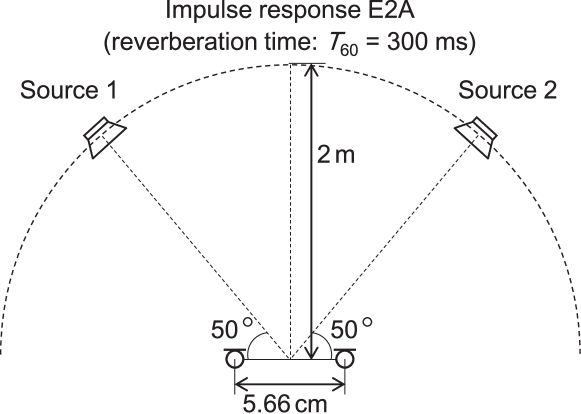
Figure 3: Recording conditions of impulse response E2A ($T_{60}=$300\text{\,}\mathrm{m}\mathrm{s}$$) obtained from RWCP database [22].

Table 2: Experimental conditions for music and speech source separation

Sampling frequency	$16\text{\,}\mathrm{k}\mathrm{H}\mathrm{z}$
Number of iterations	1000
Number of bases	20
Number of trials	10
Domain parameter	$p=0.5$
Initial demixing matrix $\bm{W}_{i}$	identity matrix
Entries of initial source model matrices $\bm{T}_{n}$ and $\bm{V}_{n}$	uniformly distributed random values

Fig. 4 shows the average SDR improvements for Music 1–Music 6. The proposed sub-Gaussian GGD-ILRMA on average outperforms the other conventional ILRMAs. This result confirms that the proposed sub-Gaussian source model is more appropriate for dealing with music signals than other conventional (super-)Gaussian source models.

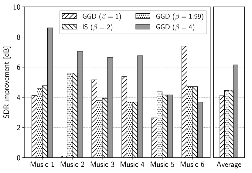
Figure 4: Average SDR improvement of GGD-ILRMA ($\beta=1$), GGD-ILRMA ($\beta=1.99$), IS-ILRMA, and proposed GGD-ILRMA ($\beta=4$) for six music signals. “Average” bar graph on right side shows average SDR improvement among six music signals for each method.

5.2 BSS Experiment on Speech Signals

We also confirmed the separation performance of the proposed sub-Gaussian GGD-ILRMA for speech signals, which are less likely to follow a sub-Gaussian distribution than music signals. We used the monaural dry speech sources from the source separation task in SiSEC2011 [24], Speech 1–Speech 4. An STFT was performed using a 256-ms-long Hamming window with a 128-ms-long shift. The other conditions were the same as those of the music source separation experiment.

Fig. 5 shows the average SDR improvements for Speech 1–Speech 4. The proposed GGD-ILRMA on average outperforms the other conventional ILRMAs even for speech signals, which are expected to be sparse and follow super-Gaussian distributions. This shows that the proposed time-variant sub-Gaussian model can appropriately model super-Gaussian signals as well as sub-Gaussian signals owing to its time-variant property, as described in Sect. 4.1.

Figure 5: Average SDR improvement of GGD-ILRMA ($\beta=1$), GGD-ILRMA ($\beta=1.99$), IS-ILRMA, and proposed GGD-ILRMA ($\beta=4$) for four speech signals. “Average” bar graph on right side shows average SDR improvement among four speech signals for each method.

6 Conclusion

We proposed a new type of ILRMA, which assumes that the source signal follows the time-variant isotropic complex sub-Gaussian GGD. By using a new update scheme called GIP-HSM, we obtained a convergence-guaranteed update rule for the demixing matrix. Furthermore, in the experimental evaluation, we revealed the versatility of the proposed method, i.e., the proposed time-variant sub-Gaussian source model can deal with various types of source signal, ranging from sub-Gaussian music signals to super-Gaussian speech signals.

.1 Derivation of Update Rule for Low-Rank Source Model

The update rules for $\bm{T}_{n}$ and $\bm{V}_{n}$ in GGD-ILRMA can be derived by the MM algorithm. In the MM algorithm, we minimize the majorization function instead of the original cost function. To derive the majorization function in GGD-ILRMA, we introduce Jensen’s inequality

$$\left(\sum_{k}t_{ikn}v_{kjn}\right)^{-\frac{\beta}{p}}\leq\sum_{k}\phi_{ijnk}\left(\dfrac{t_{ikn}v_{kjn}}{\phi_{ijnk}}\right)^{-\frac{\beta}{p}}$$ (65)

and the tangent-line inequality

$$\log\sum_{k}t_{ikn}v_{kjn}\leq\dfrac{1}{\psi_{ijn}}\left(\sum_{k}t_{ikn}v_{kjn}-1\right)+\log\psi_{ijn},$$ (66)

where $\phi_{ijnk}>0$ and $\psi_{ijn}>0$ are auxiliary variables and $\phi_{ijnk}$ satisfies $\sum_{k}\phi_{ijnk}=1$. The equalities of (65) and (66) hold if and only if

$$\phi_{ijnk} =\dfrac{t_{ikn}v_{kjn}}{\sum_{k^{\prime}}t_{ik^{\prime}n}v_{k^{\prime}jn}},$$ (67)

$$\psi_{ijn} =\sum_{k}t_{ikn}v_{kjn},$$ (68)

respectively. By substituting (8) into (9) and applying (65) and (66) to (9), the majorization function of (9) can be designed as

$$\mathcal{L}_{\mathrm{GGD}} \leq\sum_{i,j,n,k}\left(\dfrac{\phi_{ijnk}^{\frac{\beta}{p}+1}\left\lvert y_{ijn}\right\rvert^{\beta}}{(t_{ikn}v_{kjn})^{\frac{\beta}{p}}}+\dfrac{2t_{ikn}v_{kjn}}{p\psi_{ijn}}\right)+\mathrm{const.},$$ (69)

where the constant term is independent of $t_{ikn}$ and $v_{kjn}$. By setting the partial derivatives of (69) w.r.t. $t_{ikn}$ and $v_{kjn}$ to zero, we obtain the update rules (16) and (17), respectively.

References

- [1] P. Comon, “Independent component analysis, a new concept?” Signal Process., vol. 36, no. 3, pp. 287–314, 1994.
- [2] P. Smaragdis, “Blind separation of convolved mixtures in the frequency domain,” Neurocomputing, vol. 22, no. 1, pp. 21–34, 1998.
- [3] H. Sawada, R. Mukai, S. Araki, and S. Makino, “A robust and precise method for solving the permutation problem of frequency-domain blind source separation,” IEEE Trans. ASLP, vol. 12, no. 5, pp. 530–538, 2004.
- [4] H. Saruwatari, T. Kawamura, T. Nishikawa, A. Lee, and K. Shikano, “Blind source separation based on a fast-convergence algorithm combining ICA and beamforming,” IEEE Trans. ASLP, vol. 14, no. 2, pp. 666–678, 2006.
- [5] A. Hiroe, “Solution of permutation problem in frequency domain ICA using multivariate probability density functions,” in Proc. ICA, 2006, pp. 601–608.
- [6] T. Kim, H. T. Attias, S.-Y. Lee, and T.-W. Lee, “Blind source separation exploiting higher-order frequency dependencies,” IEEE Trans. ASLP, vol. 15, no. 1, pp. 70–79, 2007.
- [7] N. Ono, “Stable and fast update rules for independent vector analysis based on auxiliary function technique,” in Proc. WASPAA, 2011, pp. 189–192.
- [8] K. Yatabe and D. Kitamura, “Determined blind source separation via proximal splitting algorithm,” in Proc. ICASSP, 2018, pp. 776–780.
- [9] D. Kitamura, N. Ono, H. Sawada, H. Kameoka, and H. Saruwatari, “Determined blind source separation unifying independent vector analysis and nonnegative matrix factorization,” IEEE/ACM Trans. ASLP, vol. 24, no. 9, pp. 1626–1641, 2016.
- [10] D. Kitamura, N. Ono, H. Sawada, H. Kameoka, and H. Saruwatari, “Determined blind source separation with independent low-rank matrix analysis,” in Audio Source Separation, S. Makino, Ed. Springer, Cham, March 2018, ch. 6, pp. 125–155.
- [11] D. D. Lee and H. S. Seung, “Learning the parts of objects by non-negative matrix factorization,” Nature, vol. 401, no. 6755, pp. 788–791, 1999.
- [12] A. Ozerov and C. Févotte, “Multichannel nonnegative matrix factorization in convolutive mixtures for audio source separation,” IEEE Trans. ASLP, vol. 18, no. 3, pp. 550–563, 2010.
- [13] A. Ozerov, C. Févotte, R. Blouet, and J. L. Durrieu, “Multichannel nonnegative tensor factorization with structured constraints for user-guided audio source separation,” in Proc. ICASSP, 2011, pp. 257–260.
- [14] H. Sawada, H. Kameoka, S. Araki, and N. Ueda, “Multichannel extensions of non-negative matrix factorization with complex-valued data,” IEEE Trans. ASLP, vol. 21, no. 5, pp. 971–982, 2013.
- [15] S. Mogami, D. Kitamura, Y. Mitsui, N. Takamune, H. Saruwatari, and N. Ono, “Independent low-rank matrix analysis based on complex Student’s -distribution for blind audio source separation,” in Proc. MLSP, 2017.
- [16] D. Kitamura, S. Mogami, Y. Mitsui, N. Takamune, H. Saruwatari, N. Ono, Y. Takahashi, and K. Kondo, “Generalized independent low-rank matrix analysis using heavy-tailed distributions for blind source separation,” EURASIP Journal on Advances in Signal Processing, vol. 2018, no. 28, pp. 1–25, 2018.
- [17] R. Ikeshita and Y. Kawaguchi, “Independent low-rank matrix analysis based on multivariate complex exponential power distribution,” in Proc. ICASSP, 2018, pp. 741–745.
- [18] G. R. Naik and W. Wang, “Audio analysis of statistically instantaneous signals with mixed Gaussian probability distributions,” International Journal of Electronics, vol. 99, no. 10, pp. 1333–1350, 2012.
- [19] D. R. Hunter and K. Lange, “Quantile regression via an MM algorithm,” J. Comput. Graph. Stat., vol. 9, no. 1, pp. 60–77, 2000.
- [20] D. Kitamura, H. Saruwatari, H. Kameoka, Y. Takahashi, K. Kondo, and S. Nakamura, “Multichannel signal separation combining directional clustering and nonnegative matrix factorization with spectrogram restoration,” IEEE Trans. ASLP, vol. 23, no. 4, pp. 654–669, 2015.
- [21] D. Kitamura, “Open dataset: songkitamura,” http://d-kitamura.net/en/dataset_en.htm. Accessed 27 May 2018.
- [22] S. Nakamura, K. Hiyane, F. Asano, T. Nishiura, and T. Yamada, “Acoustical sound database in real environments for sound scene understanding and hands-free speech recognition,” in Proc. LREC, 2000, pp. 965–968.
- [23] E. Vincent, R. Gribonval, and C. Févotte, “Performance measurement in blind audio source separation,” IEEE Trans. ASLP, vol. 14, no. 4, pp. 1462–1469, 2006.
- [24] S. Araki, F. Nesta, E. Vincent, Z. Koldovský, G. Nolte, A. Ziehe, and A. Benichoux, “The 2011 signal separation evaluation campaign (SiSEC2011): - audio source separation -,” in Proc. LVA/ICA, 2012, pp. 414–422.