KEK-TH 2068
Non-Cartan Mordell-Weil lattices of rational
elliptic surfaces and heterotic/F-theory
compactifications
Shun’ya Mizoguchi1
***mizoguchi@post.kek.jp
and Taro Tani2
†††tani@kurume-nct.ac.jp
1Theory Center, Institute of Particle and Nuclear Studies, KEK
Tsukuba, Ibaraki 305-0801, Japan
2National Institute of Technology, Kurume College
Kurume, Fukuoka 830-8555, Japan
1mizoguchi@post.kek.jp
2tani@kurume-nct.ac.jp
The Mordell-Weil lattices (MW lattices) associated to rational elliptic surfaces are classified into 74 types. Among them, there are cases in which the MW lattice is none of the weight lattices of simple Lie algebras or direct sums thereof. We study how such “non-Cartan MW lattices” are realized in the six-dimensional heterotic/F-theory compactifications. In this paper, we focus on non-Cartan MW lattices that are torsion free and whose associated singularity lattices are sublattices of . For the heterotic string compactification, a non-Cartan MW lattice yields an instanton gauge group with one or more group(s). We give a method for computing massless spectra via the index theorem and show that the instanton number is limited to be a multiple of some particular non-one integer. On the F-theory side, we examine whether we can construct the corresponding threefold geometries, i.e., rational elliptic surface fibrations over . Except for some cases, we obtain such geometries for specific distributions of instantons. All the spectrum derived from those geometries completely match with the heterotic results.
1 Introduction
F-theory [1, 2, 3] has a unique feature in modern particle physics model building based on string theory. The GUT, which naturally explains the hypercharges of the observed quarks and leptons, and matter in the spinor representation of , into which all the quarks and leptons of a single generation are successfully incorporated—both are readily achieved in F-theory. F-theory models have an advantage over the heterotic models as they may evade the issue of the GUT vs. Planck scales first addressed in [4]. F-theory can also generate Yukawa couplings that are perturbatively forbidden in D-brane models [5].
Almost a decade after the first formulation of F-theory, there was considerable development in understanding the local models [6, 7, 8, 9] in terms of twisted super Yang-Mills theories or the Higgs bundles [10, 11]. One of the notable findings in the development was the mechanism of the GUT gauge symmetry breaking by the fluxes turned on the brane. A large number of studies have been carried out in local models. An incomplete list includes [12, 13, 14, 15].
Rather soon after this development, the Higgs particle was found at LHC in 2012, and the subsequent experiments showed that there was no low-energy supersymmetry. Later, the PLANCK data became also available to reveal that the energy of the inflation can be very high, even close to the GUT scale. These two new sources of knowledge have turned the focus of F-theory model building to global models. It is also known [3] that gauge symmetries in F-theory arise when the Mordell-Weil rank is nonzero, that is, when there are nontrivial global sections. This is in sharp contrast to nonabelian gauge symmetries, which can be solely determined by the singularity in the local model. Recent works on global models include [16, 17, 18, 19, 20, 21, 22, 23, 24, 25, 26, 27, 28, 29, 30, 31, 32, 33, 34, 35, 36, 37, 38, 39, 40, 41, 42, 43, 44, 45, 46, 47, 48, 49, 50].
For K3 surfaces, the Mordell-Weil rank varies depending on its Picard number. In contrast, the Mordell-Weil rank of a rational elliptic surface is always 10. Its Mordell-Weil group is known to be endowed with a lattice structure, and the possible pairs of the singularity and the corresponding Mordell-Weil lattice have been classified into 74 types [51]. Roughly speaking, the singularity lattice and the Mordell-Weil lattice are the orthogonal compliment of each other in the root lattice. In a typical case, the Mordell-Weil lattice coincides with a weight lattice of some semi-simple gauge group of the instantons in the dual heterotic string theory, and the singularity lattice is that of the unbroken gauge group. However, it is interesting to note that in the other cases the inner product matrix of the Mordell-Weil lattice is none of the (inverse of the) Cartan matrices of simple Lie algebras, nor is it their direct sum. It is these non-Cartan type Mordell-Weil lattices that we focus on in this paper. In fact, these are the cases where the gauge instanton includes some factor(s).111As there are no such things as “ instantons” in the ordinary four-dimensional noncompact Euclidean space, that might sound bizarre, but in a complex compact space they are nothing but line bundles with a nonzero first Chern class.
We are particularly interested in the explicit forms of the Weierstrass equations of this special class of rational elliptic surfaces with a section 222 Incidentally, the very same objects were studied in late 90’s as Seiberg-Witten curves for E-strings [52, 53, 54, 55, 56, 57, 58], though these rational elliptic surfaces were not supposed to be further fibered over anything then. A recent work on non-Cartan MW lattices for rational elliptic surfaces (and not their fibrations) is [59]. which are fibered over to form a complex threefold. This means that the parameters of the Weierstrass equations are sections of some line bundles over [3].333 Although we consider in this paper rational elliptic surfaces fibered over , the Weierstrass equations we obtain can be readily converted to those for a fibration over a complex two-fold by simply replacing a degree polynomial in the affine coordinate of the , with a section of with and , where is the anti-canonical bundle of and is the twisting line bundle determining the normal bundle of the fiber , which is the base of the rational elliptic surface. For further explanation of this correspondence, see [60]. Each of these geometries is regarded as a part of an elliptic K3 fibration in the stable degeneration limit [61, 62, 63] , and hence as a “1/2 CY threefold” since two such complex manifolds can be glued together into a K3-fibered Calabi-Yau threefold (CY3).
In this paper, we will specifically consider a class of rational elliptic surfaces, and their fibrations over , which satisfy the following criteria:
-
1.
The Mordel-Weil lattice is neither a weight lattice of some semi-simple Lie algebra, nor is it a direct sum of such a weight lattice and a torsion.
-
2.
The singularity lattice is a sublattice of .
There are ten types of such rational elliptic surfaces in the Oguiso-Shioda classification, which are summarized in Table 1 (See section 2).
To find an equation representing a “rational-elliptic-surface (RES)-fibered” complex threefold over whose fiber rational elliptic surface belongs to this class, our strategy is to realize in the geometry the singularity of lattice associated to a given . First, we start from No.7 with singularity , which is not a non-Cartan type, and construct the corresponding CY3 with K3 fibration. We then successively tune the complex structures (“unHiggsing”) to achieve the necessary singularities of the respective types given in Table 1. Next, we map the obtained K3-fibered CY3’s to RES-fibered geometries. We carefully construct this map so that it does not change the structure of the singularity. Through this strategy, we can successfully obtain the equations for all the series (upper rows in Table 1) and some (No.22 and No.29) of the series (lower rows in Table 1). We will also discuss why it is hard to find the equations for the remaining cases. We note that the equations for series cannot be obtained by using Tate’s form and we need to work in the Weierstrass form. This is because, if the coefficients of Tate’s form are assumed to have the necessary factors required from each singularity of the series, then the total degrees of some (including and ) would exceed , leading additional unwanted singularities.
We also compute the massless spectra of the dual heterotic string compactifications whose vector bundles are supposed to be determined by the RES-fibered spaces above [2, 3, 64]. For all cases except No.45 in Table 1, the instanton gauge group in the dual heterotic string theory has two or more irreducible group factors. In particular, we will see that specified by a non-Cartan Mordel-Weil lattice is typically a product of a semi-simple group and one or more group(s). Thus one can distribute the total instanton numbers to each group factor. Although in principle there is no problem in applying the index theorem to these cases, the subtlety is that the multiplicities of some massless hypermultiplet then become fractional unless the instanton number is a multiple of some particular non-one integer. We will show why the instanton number cannot take an arbitrary integral value but must be a multiple by examining the orthogonal decomposition of the root lattice. This gives us a consistent integral number of hypermultiplets. For the cases of , more than one choices of the number of direction(s) are possible. In such cases, we obtain more than one spectra for a given (and hence for a given ). We find that the spectrum is more general when the number of direction(s) is larger.
While it is possible to compute heterotic indices for the cases of distributed instantons, it is a nontrivial problem to obtain the equations for the RES-fibered spaces corresponding to such particularly distributed instantons. We will explain for the No.7 case, which is a Cartan type, how we can obtain the equations for an arbitrary distribution of instantons, and show the complete match of the six-dimensional massless spectra read off from the Weierstrass equations on the F-theory side and those obtained by the index computations on the heterotic side. On the other hand, for every case of the non-Cartan type, where we have succeeded to find an equation for the RES-fibered space, we also show that the spectrum read off from the equation agrees with that of the dual heterotic theory for a special choice of instanton distribution.
The outline of this paper is as follows: In section 2, we begin with an introduction to the non-Cartan type Mordell-Weil lattices. In section 3, we first review a general method to compute heterotic indices in six dimensions and demonstrate how it works in particular examples. We also discuss there why the instanton numbers must be a multiple of some particular non-one integer in general. In section 4 we review the basic facts on the six-dimensional F-theory/ heterotic duality, and explain our strategy to obtain the equation for a RES-fibered threefold having a non-Cartan Mordell-Weil lattice. In section 5, we start the construction by the No.7 case of the Oguiso-Shioda classification to obtain the equation for the case of a particular instanton distribution. We then deform this equation in an appropriate way to find the equations for threefolds with arbitrarily distributed instantons. The match of the spectra is also verified there. Sections 6 and 7 are devoted to the considerations of the RES-fibered threefolds for the the cases of the series and the series, respectively. Finally we summarize our conclusions in section 8. In appendix A and B, we present the detail of the heterotic index computations for the and the series, respectively. Appendix C shows the explicit forms of the functions , of the Weierstrass equations and the discriminant for various cases considered in the text.
2 Models with non-Cartan type Mordell-Weil lattices
It is known that a rational elliptic surface possesses a lattice structure, called the Mordell-Weil lattice . ( is the field over which is defined.) When has no singularity, is the self dual lattice. When has a singularity of an type with root lattice , is reduced, roughly speaking, to the orthogonal complement of in . More precisely, is the dual lattice of accompanied with a torsion part:
| (2.1) |
where ∗ denotes the dual lattice. satisfies
| (2.2) |
In the context of the duality between F-theory and heterotic string, the root lattice of the singularity in corresponds to the gauge symmetry , while the orthogonal complement corresponds to the gauge bundle of the heterotic string. The decomposition (2.2) is then interpreted as
| (2.3) |
In other words (apart from the torsion part),
| (2.4) |
The Mordell-Weil lattices are classified into 74 patterns [51]. In many cases, is a weight lattice of some type Lie algebra or a direct sum thereof, but there are some special cases where is not a weight lattice of any type Lie algebra. In these cases is also not a root lattice of any type, and neither is the gauge bundle of the heterotic string. Let us call these Mordell-Weil lattices and the corresponding gauge bundles “non-Cartan type”. In this paper, among them, we will study the cases listed in Table 1, where is a subalgebra of and is torsion free.
| No. | ||
|---|---|---|
In the table, is a matrix representing the lattice . The inverse representing the dual lattice , or equivalently, the gauge bundle , takes one of the following non-Cartan forms:
| (2.5) |
are the weight lattices of . denotes the one-dimensional lattice with lattice spacing . Its dual lattice has a non-Cartan form unless , in which the lattice becomes the weight lattice.
In terms of heterotic string, the two series in Table 1 are obtained by Higgsing the gauge group (No.25) and (No.45), respectively. Their Higgsing chains are summarized as follows:444 (No.14 of [51]) belongs to the Higgsing chain of , but we excluded it from Table 1 because it has , which is not the non-Cartan type. (the subscripts are the numbers in Table 1)
| (2.6) |
3 Heterotic index computations
3.1 General method
We will first quickly review the general method to compute the heterotic spectrum in six dimensions.
The Dirac index for a six-dimensional compactification of heterotic string theory on a complex 2-fold is given by
| index | (3.1) |
where is the A-roof genus of the tangent bundle of the complex 2-fold on which the heterotic string is compactified, and is the Chern character of the vector bundle over . The number of hypermultiplets is given by of the index, where the overall minus sign is a convention and the factor of 1/2 is due to the fact that the heterotic gaugino is a Majorana-Weyl spinor in ten dimensions.
We consider the cases where the instanton takes values in a subgroup of, say, the first factor of to leave the centralizer subgroup of in unbroken. We are particularly interested in the cases where contains some factors. As in [65], let the of be decomposed into the representations of as
| (3.2) |
where and are irreducible representations of and , respectively. Using the fact that , the number of hypermultiplet in a representation of (and of ) is given by [65]
| (3.3) | |||||
where is the instanton gauge field 2-form taking values in (the Lie algebra of) . The trace is taken in the representation .
The equation (3.3) is still a correct formula even for the cases where contains some factors. Since
| (3.4) | |||||
due to the anomaly cancellation condition, where are the labels to distinguish the factors, we see that the second term of (3.3) is nothing but times the contribution of each representation to the total instanton number (=24, taking the factor of 1/2 into account). The normalizations of the traces and charges are determined once the instanton number of each irreducible group factor of is specified.
3.2 Example 1 : (No.25)
In this case one can take as . Let the instanton numbers of and be and , respectively, so that the total instanton number of is . Then we have 555The subscript “K3” for the integral is omitted below.
| (3.5) |
The adjoint representation of is decomposed as
| (3.6) | |||||
where the subscripts denote the charges. This yields
| (3.7) | |||||
where are the representation matrices of , and is the sum of the charge squares. As we assumed above, the first term is equal to , whereas the second term is . Therefore we have
| (3.8) |
which means that (Note the factor of in eq.(3.3)) a representation of contributes , whereas each -charge component contributes , to the multiplicities of hypermultiplets transforming in the corresponding representation.
As an illustration let us compute . This is computed as
| (3.9) | |||||
Note that the 3rd ( instanton) term is multiplied by 2 because each component of contributes to the index.
Since is equal to (3.9), and there is no distinction between and in six dimensions, the total multiplicity of is in all
| (3.10) |
This becomes an integer if and only if the instanton number is a multiple of 7. So writing , we have
| (3.11) |
The computations of the multiplicities for other representations can be worked out similarly. The result is summarized in Table 2.
| Representation | Multiplicity |
|---|---|
| ( vector) | |
Finally, we would like to comment on the computation in [66] of the heterotic string matter spectrum with an gauge group, which is different from ours but led them to the same result as that derived here. Since the multiplicities are not integers when is a multiple of 7, they consider instead of with an extra and assumed a contribution of this additional to the multiplicity of the singlet (See the top row of Table 8 of [66], where the multiplicity of 1 contains the term despite that the singlets (the first two terms of (4.8) in [66]) are not charged under the ). This must commute with both the and the and must be different from the original factor in , but obviously, there is no room for such an extra in as the rank is already exhausted.
3.3 Orthogonal decompositions of the root lattice: Why a multiple of seven?
The fact that the U(1) instanton number must be a multiple of seven can be understood by an orthogonal decomposition of the root lattice. Let (i=1,…,9) be a set of orthonormal vectors of nine-dimensional flat Euclidean space with inner product
| (3.12) |
Then the following set of vectors on an eight-dimensional hyperplane normal to form the set of root vectors of :
| (3.13) | |||
| (3.14) |
This fact can be most easily verified by considering Freudenthal’s realization of the algebra [67, 68]. The first line (3.13) is the set of root vectors of , while the second line (3.14) is the root vectors corresponding to the rank-3 tensors of . Using this presentation of roots, one can easily see where the roots of are embedded and which root vector is the one corresponding to the generator. As the root vectors of one can take
| (3.15) |
and the roots of is then
| (3.16) |
In the root lattice generated by the vectors (3.13) and (3.14), the orthogonal lattice normal to the and lattices spanned by (3.15) and (3.16) is one-dimensional, generated by
| (3.17) |
The length square of (3.17) is 14, which is 7 times as large as the simple-root length square. This explains why the instanton number of is a multiple of 7.
Note that the junction lattice [69], which is the inverse of the matrix of section parings, is given in the present case as
| (3.20) |
This can be made diagonal by the change of basis
| (3.29) |
which agrees with the above consideration.
3.4 Example 2 : (No.17)
In this case, and we can take one or two direction(s) in . Namely, or . The gauge symmetry is the same () for these two gauge bundles, but the resulting spectra are different. As we will explain below, the spectrum for is more general than the one for .
3.4.1 The case when
The junction lattice is
| (3.33) |
As , we allow the instantons to live also in a different as well as the for No.25 in the previous section, so that the is further broken to . The instanton numbers are assumed to be , and for , and , respectively. The decomposition of in representations of these subgroups is shown in Table 3.
| Rep. of | Rep. of (in ) | charge | charge |
|---|---|---|---|
| 1 | 0 | 0 | |
| 1 | 0 | 0 | |
| 1 | 0 | 7 | |
| 1 | 0 | ||
| () | 1 | 0 | 0 |
| 2 | |||
| 1 | |||
| 2 | |||
| 1 | |||
| 2 | |||
| 1 | |||
| 2 | |||
| 1 | |||
| 1 | |||
| 1 | |||
| 1 | |||
| 1 | |||
| 1 | |||
| 1 | |||
| 2 | |||
| 2 | |||
| 2 | |||
| 2 | |||
| 2 | |||
| 2 | |||
| () | 1 | 0 | 0 |
| 3 | 0 | 0 |
In the present case
| (3.34) |
and
| (3.35) |
so that
| (3.36) |
The spectrum for No.17 is similarly obtained as shown in Table 4.
| Representation | Multiplicity |
|---|---|
| ( vector) | |
| ( vector) | |
For to be integer, the general solution is
| (3.37) |
so that
| (3.38) |
therefore or need not necessarily be a multiple of or in general. The orthogonal decomposition of the junction lattice is
| (3.51) |
which implies that the minimal charge square (measured by the root space inner product) is 35 times (and not 70 times) as large as that of the factor. This is almost equivalent to the condition for the integrality of the multiplicities, but the latter is “twice as” severe.
3.4.2 The case when
We can see the Cartan matrix in the right-down block of
| (3.56) |
and we can also take as . Orthogonal decomposition of the junction lattice is
| (3.69) |
In representations of this , the adjoint is decomposed as shown in Table 5.
| Rep. of | Rep. of | charge |
|---|---|---|
| 1 | 0 | |
| 1 | 0 | |
| 3 | ||
| 8 | 0 | |
| 1 | 0 | |
| 3 | ||
| 1 | ||
| 3 | ||
| 1 | ||
| 1 | ||
| 1 | ||
| 3 |
We assume instantons in and in . Then since
| (3.71) |
we obtain
| (3.72) |
where () are the Gell-Mann matrices. Incidentally, is the “hypercharge” that breaks one of of into . The spectrum is as shown in Table 6.
| Representation | Multiplicity |
|---|---|
| ( vector) | |
| ( vector) | |
Here we have defined so that the multiplicities become all integers when the instanton number is a multiple of (which is when is an integer).
Note that this spectrum coincides with the spectrum shown in Table 4 provided that the replacement
| (3.73) |
is made. Thus the spectrum for is “three times” as restrictive as that for .
The index computations for other cases can be done similarly. We summarize the relevant results (No.19 and No.12 for series and No.29 and No.22 for series) in Appendices A and B.
4 Geometries for non-Cartan Mordell-Weil lattices
Suppose that a non-Cartan Mordell-Weil lattice (non-Cartan gauge bundle ) is given. To construct the corresponding geometry, which is a rational elliptic surface fibered over , we first construct a K3-fibered CY3 with the singularity (gauge symmetry ) paired with the given . Then, we map the CY3 to a RES-fibered geometry.
4.1 CY3 in six-dimensional F-theory/heterotic duality
We first review the construction of a CY3 for six-dimensional F-theory compactification [2, 3, 70]. heterotic string/K3 contains 24 instantons. Suppose of them take values in a gauge bundle in the first and the gauge symmetry is broken to , while the other instantons take values in another gauge bundle in the second and the gauge symmetry is broken to . It has been known [2] that the corresponding dual F-theory geometry is a K3-fibered CY3 over and at the same time is an elliptic fibered CY3 over the Hirzebruch surface with singularities and . The Weierstrass form is given by
| (4.1) |
with
| (4.2) |
is a fibration over the base , whose coordinates are and , respectively. and are polynomials of with homogeneous order . Let us write the fiber coordinate in a homogeneous form . Under the action , the other coordinates transform as
| (4.3) |
Also, for the base coordinate , the action gives
| (4.4) |
The Weierstrass form (4.1) is homogeneous under these actions with degrees and .
Singularities and are realized by demanding that , and the discriminant ,
| (4.5) |
have suitable vanishing orders near and (see Table 7).
| ord | ord | Fiber type | Singularity type | |
|---|---|---|---|---|
| smooth | none | |||
| none | ||||
| non-min | — |
For realizing gauge symmetry in six dimensions, these Kodaira fibers should satisfy the so-called split conditions [70], which we will require in our construction since all the gauge symmetries that we would like to achieve (Table 1) are of the type. (The explicit form of the split condition can be seen in Table 8 below.)
The last row of Table 7 expresses the singularity that cannot be resolved by any blow up of the fiber. To resolve it, blowing up the base is required and an additional tensor multiplet appears in the spectrum. Such a theory does not have a heterotic dual in the perturbative regime, and hence is not the subject of our study.
The elliptic fibration over can also be written in Tate’s form [70, 71]
| (4.6) |
where are polynomials of and . Because of the homogeneity under (4.3), are degree polynomials in :
| (4.7) |
Here are polynomials of . Their degrees are determined by the homogeneity under (4.4) as
| (4.8) |
Discriminant is given by
| (4.9) |
where () are defined in terms of as follows:
| (4.10) |
Singularities and are realized by requiring () to vanish at suitable orders of , known as Tate’s algorithm (see Table 8).
| ord | ord | ord | ord | ord | ord | Coefficient of | Fiber | Group |
|---|---|---|---|---|---|---|---|---|
| — | ||||||||
| — | ||||||||
| [ | non-min | — |
The vanishing orders of not only determine the type of the local singularity but also control its global structure. We listed in Table 8 the fibers for which the split condition is satisfied (the subscript “s” is attatched 666The fibers without subscript “s” in the Table have at most only one exceptional divisor, and hence are necessarily of the split type.). The first six columns of the table represent the lowest orders of and in . The next column is the coefficient of , where (or ) represents the coefficient of in . The “split conditions” for Kodaira fibers are the conditions that the discriminants (4.5) should be the same forms as in this column. Last two columns are the corresponding fiber degeneracy and the singularity type.777 To realize the groups with dagger, one more condition should be fulfilled. There are some polynomials and such that (here denotes ) The last row of the table expresses the singularity that never be resolved by blowing up the fiber.
4.2 Mapping CY3 to RES-fibered geometry
The Weierstrass form of a rational elliptic surface is given by
| (4.12) |
where and are sections of and on the base and have the form
| (4.13) |
Suppose that we are given a CY3 with the Weierstrass form (4.1), whose and are sections of and on as in (4.2), yielding a K3 fibration. By using their coefficients for and for , one can construct a geometry with a Weierstrass form
| (4.14) |
where
| (4.15) |
with discriminant
| (4.16) |
Here we regard and as sections of and on (with coordinate ). Then the resulting geometry is a rational elliptic surface fibered over (with coordinate ). This gives the map from the K3-fibered CY3 to a RES-fibered geometry:
| (4.17) |
When the rank of is large, we have to do a slight modification to and in order that the map does not change the singularity . For example, for with , the above procedure maps of a CY3 to the same in a RES-fibered geometry, but for , the naïve mapping changes the singularity. The explicit form of a CY3 with is given by [66]
| (4.18) |
In this CY3, and the gauge symmetry is . After mapping to and and calculating , one can see that , i.e., the singularity is reduced by the map. The source of this reduction is . Although is the coefficient of the term higher than in , it also appears in the term in . Thus, after the map , it is still contained in . By setting this polynomial to zero in , one recovers and the singularity remains to be .
In summary, the map (4.17) is obtained by first replacing and to and , and then regarding and as sections of and of , and finally setting to zero the polynomials which constitute the coefficients of the terms higher than in and in and are still contained in and even after the map . Hereafter, the resulting , and will be denoted by , and .
This last step, however, does not work for some CY3 with sufficiently large rank . In such cases, one cannot recover the original singularity of CY3 in the RES-fibered geometry and the map (4.17) does change the singularity.
There are two such cases. In the first case, additional singularities other than are produced by the map. As an example, let us consider a CY3 with constructed by using Tate’s algorithm. The orders of in (4.7) are set to be (see Table 8). Its Weierstrass form is obtained by using (4.10) and (LABEL:eq:TateWeierstrass). As a result, is realized. Mapping to and , one finds that . One can see that and contain the following polynomials which constitute the coefficients of the terms higher than in and in :
| (4.19) |
Setting these polynomials to zero, one recovers , but this singularity is accompanied by additional singularities. Explicitly, has a factorized form
| (4.20) |
with
| (4.21) |
Since the degree of is 8 , we can write . Then we obtain
| (4.22) |
At , in is enhanced to 2. Also, one can see that at these loci, yielding fibers. Thus an additional gauge symmetry appears along each line perpendicular to where the singularity exists. To explain the origin of such additional singularities, let us go back to Tate’s algorithm and focus on the orders of and , which are 4 and 8 for . It means that contains and contains . In and , are not contained since they only appear in and in the terms higher than and . Also, and do not contain , since they are set to zero (4.19). It means in and . Then, from (4.9) and (4.10), discriminant has a factorized form , leading to unwanted additional singularities (4.20). In general, when the orders of and in Tate’s algorithm exceed and simultaneously, additional singularities appear in the resulting RES-fibered geometry.
In the second case, the map (4.17) changes the singularity type of the fiber at . This occurs when the singularity in a CY3 is not contained within one () but spreads into the other (). For example, let us consider again, but take another CY3 which is different from the one obtained from Tate’s algorithm presented above and is constructed by working in the Weierstrass form directly. As seen from (LABEL:eq:TateWeierstrass), a CY3 in Tate’s form is always rewritten in the Weierstrass form, but the inverse is not the case in general. This means that there may exist models that are described only in the Weierstrass form and have no Tate’s counterpart (see e.g., [72]). Hence the appearance of additional singularities (4.22) in RES-fibered geometry may be an artifact in Tate’s form. There may exist another model that cannot be reached by Tate’s algorithm and for that CY3 additional singularity may not arise after the map (4.17). A candidate of such a CY3 is the one constructed in [66]. The explicit form is given by 888This is the case given by setting and in [66].
| (4.23) |
with an irreducible polynomial
| (4.24) |
The important difference from the CY3 constructed by Tate’s algorithm is that the terms higher than in or in contain a term written by only the polynomials that are needed to express and . It is contained in of . It is the sign that this singularity can not be realized in a rational elliptic surface fibration but we need a full-fledged K3 fibration. As a result, the map (4.17) changes the singularity as follows. Mapping and to and , one obtains . The and terms of contain the polynomials
| (4.25) |
which are the coefficients of the terms higher than in and in . Setting them to zero, we have . Thus, the singularity is reduced by the map (4.17).999If we set the term of to zero in advance, i.e., if we set or in (4.23), the singularity is contained within one . In these cases, mapping to and gives and setting and (4.25) to zero gives . However, the resulting has a factorized form and additional singularities arise. That is, these cases result in Tate’s case described above. Explicitly, for and for .
5 Geometry for (No.7)
The starting point of our construction is the CY3 for the model. It is No.7 of [51] and its Mordell-Weil lattice is . As we claimed in the previous section, there are models that can be written in the Weierstrass form but cannot be written in Tate’s form. Therefore, we use the Weierstrass form throughout this paper, but for the model, we start from Tate’s form and convert it to the Weierstrass form.101010We can alternatively start from the Weierstrass form for and Higgsing it to derive the model, but the construction by using Tate’s algorithm is more straightforward. This is because Tate’s algorithm is more convenient for realizing product gauge groups.
5.1 The heterotic spectrum
In this model, since () is the Cartan type, the heterotic spectrum is determined in a standard way. Let us divide the instantons taking values in into each factor and such that
| (5.1) |
By using the index theorem, we obtain the spectrum as in Table 9.
| Representation | Multiplicity |
|---|---|
| ( vector) | |
The number of the hypermultiplets is given by
| (5.2) |
while the number of vector multiplets reads . Therefore, anomaly cancellation condition is satisfied as
| (5.3) |
5.2 case
It is necessary to put the singularities on three different lines. We first put the singularity at . From Tate’s algorithm (Table 8), the orders are given by , and hence should satisfy
| (5.4) |
Next we put the second on another line. This line is taken to be
| (5.5) |
is shifted by an order polynomial , so that is homogeneous under the transformation (4.4). To realize the singularity at , we re-expand in terms of as
| (5.6) |
and impose on the same conditions as in (5.4),
| (5.7) |
Finally, we place the third at
| (5.8) |
and re-expand as
| (5.9) |
and impose
| (5.10) |
The resulting form of ’s are given as follows:
| (5.11) |
where are written by , and . To translate this Tate’s form into the Weierstrass form, we calculate (4.10). Although have complicated dependence of , and , one can redefine so that they are arranged to have simple forms:
| (5.12) |
Substituting them into (LABEL:eq:TateWeierstrass), we obtain and in terms of . To arrange so that the middle polynomials and have simple form, we further redefine as
| (5.13) |
Similarly, we redefine with by subtracting dependent terms:
| (5.14) |
Moreover, we found that and can be discarded from and without any effect on the singularity structure. As a result, we obtain the following form:
| (5.15) |
Here the dependence on and is included only through the symmetric polynomials as it should be because the lines of singularity can be replaced with each other:
| (5.16) |
The discriminant has the form
| (5.17) |
where is an irreducible polynomial written by , and . The leading expansion is given by
| (5.18) |
We map these and to and . Then and contain the polynomials
| (5.19) |
which constitute the coefficients of the terms higher than in and in . Setting them to zero, one obtains a RES-fibered geometry. One can see from the explicit forms of , and that the singularity remains to be (see (5.22), (5.23) and (5.24) below).
From this geometry, let us extract the matter spectrum. Singlets correspond to the moduli space of the gauge bundle , which is identified with the complex moduli of the geometry, except for the middle polynomials and belonging to the geometric moduli of the heterotic K3. The number of singlets, therefore, is the number of degrees of independent polynomials contained in and except and . Charged matters are localized at codimension two loci of singularities on the base space. Suppose the generic codimension one singularity is and it enhances to at a codimension two locus. Then there is a matter in a representation corresponding to the off diagonal part of .111111It is justified in the type IIB picture by using the notion of string junctions [73].
In the present case, and contain the following six independent polynomials (apart from and , which are not counted because they correspond to the middle polynomials and ):
| (5.20) |
The degree of each polynomial is given by (4.8). The number of the singlet (neutral hypermultiplet) is thus calculated as
| (5.21) |
where is the overall rescaling.
To see where and how the singularity enhances, we expand and near each of the three lines and . The results are
| (5.22) |
| (5.23) |
| (5.24) |
Here
| (5.25) |
and and are degree irreducible polynomials. We represented as the factors irrelevant to the symmetry enhancement for simplicity. From these expansions, one can read the loci and types of enhancements, and then one finds what kind of representations of matters appear at those points. The result is given by
| (5.26) |
This table is obtained as follows. We first pay attention on the leading term of in (5.24). The coefficient is a product of several factors. If one of them vanishes, the order of enhances. The list of such factors are shown in the first column and its degree is shown in the second column. When a factor vanishes, not only the order of but also the orders of and enhance in general. To what extent they will enhance can be read from (5.22), (5.23) and (5.24) and given in the next three columns. The resulting enhancement can be read from Table 7 and is shown in the next column. The associated matter representation is given in the last column, where the three entries correspond to the three at , and in this order. As we can see, unresolvable singularity does not appear anywhere.
Let us give some comments. Consider in the first row. In this case, the fiber degeneracy is enhanced from to , but the singularity does not change and remains to be . Therefore, there exists no matter at these points. The same is true for and . When (the fifth row), the orders of expansions around and simultaneously enhance to , while the orders of do not change. This reflects the fact that the two lines and intersect at , giving rise to matter in the bi-fundamental representation . A similar thing is true for and .
5.3 case
We next construct a CY3 for general distributions of instantons and then map it to a RES-fibered geometry. As seen in the previous section, Tate’s algorithm gives the case only. This means that the case is not obtained by Tate’s algorithm and we have to use the Weierstrass form. So we start from the Weierstrass form (5.15) for the case and deform the equation appropriately. In order to know how to deform it, we use one particular information from the heterotic spectrum in Table 9 as an input. The only input data is the appearance of half-hypermultiplets in the tri-fundamental representation . We determine the CY3 so that they are contained. As we will show below, it turns out that this requirement uniquely determines the CY3. After mapping to a RES-fibered geometry, we derive the full spectrum. The resulting F-theoretic full spectrum perfectly matches with the heterotic full spectrum (not only the part we used as an input).
It is expected that tri-fundamental representation is localized at a triple intersection point of three lines of singularity. For a triple intersection point to exist, and need to share a common solution, that is,
| (5.28) |
Therefore, and have a common factor. Writing this factor as , we have
| (5.29) |
Three lines intersect at points satisfying and .
The next question is how much the gauge symmetry is enhanced where a tri-fundamental appears. As we argue below, it should be
| (5.30) |
Let us first look at the branching of :
| (5.31) |
The tri-fundamental is contained in the off-diagonal elements. Moreover, there is a maximal embedding , whose branching is given by
| (5.32) |
In the branching of the maximal embedding with , the representation of which is combined with of
is a pseudo-real representation.
In the present case (5.32), the tri-fundamental representation of is pseudo-real,
forming a half-hypermultiplet .121212We list below the other examples of arising half-hypermultiplets
given in [70]. Why half-hypermultiplets appear in these cases has been explained from string junctions’ point of view [73].
In order that the singularity is enhanced to at , we have to tune the geometry so that at . Let us first notice that at . One can then easily see from (5.15) that at if and only if is factorized as (recall that the degree of is given by (4.8))
| (5.33) |
Calculating explicitly, however, we find that it is over-enhanced to at . We have to suppress it to while keeping . To absorb the excessive factors of in , we have to factorize for at least one polynomial as
| (5.34) |
But as a side effect, this replacement would cause poles in several terms of and . To keep the orders of and fixed, it should be accompanied with the factorization of other polynomial
| (5.35) |
Take a term in or . If is contained in the coefficient of that term as a product , we can “ interchange the factor ” to absorb the pole as [66]
| (5.36) |
On the other hand, if is contained as for some , the pole cannot be cancelled.
Among the polynomials contained in the CY3 for case (5.15), only those listed in (5.20) can change the singularity type near . and are already factorized. The remainings are , and . Among them, is the one that should be divided by . The reason is as follows. Substituting (5.29) and (5.33) into (5.15), we obtain
| (5.37) |
where we defined the reduced symmetric polynomials as
| (5.38) |
Let us look at the term. It contains as . This term cannot be eliminated by any redefinitions of other polynomials in the term. Since it has the form , the interchange of (5.36) does not work. We therefore cannot remove the negative power that would arise if we imposed . The same argument holds for the polynomial contained in the term. As a result, we are forced to set . In this case, the procedure of interchanging does work. To apply it, we have to do in advance some redefinitions of polynomials so that appears in and as the form .
One can check from (5.15) the following fact: if was imposed, negative power terms would arise only at in and , in . Consider the terms in first. The negative powers of arise from
| (5.39) |
In order to have the form , we should redefine
| (5.40) |
Next, we rewrite the terms in by using instead of . The negative powers of come from
| (5.41) |
It requires the redefinition
| (5.42) |
Now we are ready to perform the interchange of . It is given by
| (5.43) |
The remaining sources of negative powers of are contained in the terms in . Substituting all the factorizations above into (5.15), one finds that the worst terms are proportional to and given by
| (5.44) |
The negative power is cancelled if and only if is proportional to , i.e.,
| (5.45) |
One can show that all these factorizations and redefinitions not merely cancel the terms,131313Via the replacement (5.43), no pole arises in higher order terms. It is because we subtracted the dependent terms in advance in (5.14). but indeed realize just the desired order at . Also, has the form
| (5.46) |
where is the same polynomial as given in (5.17) and is still irreducible after the above factorizations and redefinitions. To summarize, we obtained a CY3 with enhancement at points by imposing on (5.15) the factorizations (5.29), (5.33), (5.43), (5.45) with the redefinitions (5.40), (5.42).
After mapping and to and and then setting the polynomials (5.19) to zero, one obtains a RES-fibered geometry with . The explicit forms of , and are given in Appendix C.1.
We have derived a RES-fibered geometry whose spectrum contains half-hypermultiplet . However, it is not obvious whether the geometry reproduces the other part of the spectrum in Table 9. We will show this is the case. The number of singlets is determined by the independent polynomials. They are the following 7 polynomials defined above:
| (5.47) |
The number of the singlets are given by
| (5.48) |
Apart from the corresponding to the overall rescaling, one more is performed, because we can choose the leading coefficient of as 1 when factorizing and . If we counted the degrees of freedom of as and those of as , it would be an overcounting.
The charged matter spectrum is derived in Appendix C.1 by using the series expansions of and near each of the three lines and . The resulting charged matter multiplets (C.84) together with the singlets (5.48) give the total spectrum as
| (5.49) |
which perfectly reproduces the heterotic result (Table 9).141414The procedure of constructing geometry for general instanton distribution described in this subsection is applicable to other cases where the gauge bundle is divided into components . We have studied models whose ’s are all Cartan types. There are 7 such cases out of 74 Oguiso-Shioda classification: Nos.7,10,11,14,15,18 and 26. Among them, CY3 of No.15 and No.26 have been constructed in [60]. We have examined the other cases and have constructed the CY3 of Nos.7,10,11 and 18 with general instanton distributions. For each case, the F-theoretic spectrum precisely coincides with the heterotic spectrum. However, we have not succeeded to construct CY3 for No.14 yet.
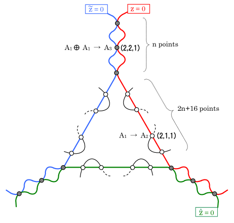
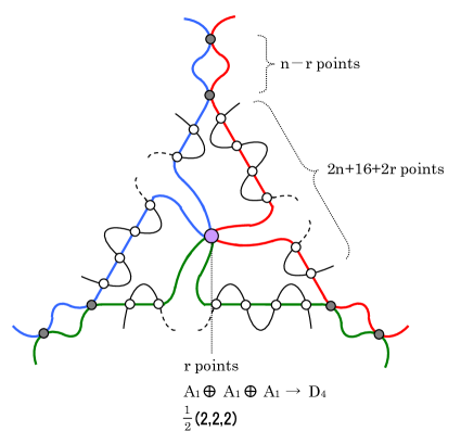
A brief sketch for the structure of the symmetry enhancement is depicted in Figure 1. The curves express the discriminant locus (the shapes are not accurate). Each matter is localized at each intersection point.
|
5.4 Looijenga’s theorem
Our geometry not only reproduces the heterotic spectrum but also encodes the structure of the moduli space of the gauge bundle . On the heterotic side, Looijenga’s theorem claims that the moduli space is parameterized by the sections (we consider the six-dimensional case)
| (5.50) |
Here is the degree of the independent Casimir of ( for ), and is the coefficient of the -th coroot when the lowest root is expanded ( for ). is the anti-canonical line bundle of the base of the heterotic K3 and is the “twisting” line bundle over . Explicitly,
| (5.51) |
where corresponds to the instanton number. Therefore, degrees of with respect to the coordinate of is given by
| (5.52) |
is identified with the coordinate of the base of , i.e., the variable of polynomials .
In the present case, with instanton numbers . Then we find that the sections in Looijenga’s theorem exactly match the 7 independent polynomials (5.47) describing the geometry on the F-theory side (see Table 10).
| deg | Polynomial | ||||
|---|---|---|---|---|---|
This correspondence is also valid for . When , the order of the polynomial becomes 0 and the independent polynomials are reduced to those of the case (5.20). In other words, the geometry for the case already captures the structure of the moduli space of the bundle . In the following discussion, we concentrate on the case.
6 Geometry for non-Cartan series
We have constructed the CY3 for in the previous section. This is No.7 and is not contained in Table 1, but by unHiggsing the first successively, we obtain the CY3 for No.12 in the series and the CY3 for No.22 in the series as
| (6.1) |
CY3’s for other cases can be obtained by further unHiggsing them. Once we obtain a CY3 for each case, we then map it to a RES-fibered geometry, extract the matter spectrum and compare it with the heterotic result given in Section 3, Appendix A and Appendix B.
6.1 (No.12)
Let us enhance the first of to . The discriminant for with is given by (see (5.17)). To enhance the first factor, we impose that is factorized as
| (6.2) |
where should be an irreducible polynomial. For this, we require that the constant term of vanishes. From (5.18), the condition is
| (6.3) |
A solution is , but it is not suitable. As seen from the explicit form of and (5.15), enhances the orders not only of but also of and near to be . The fiber degeneracy enhances as , but the singularity is kept fixed as , not enhance to . Thus we have to require the other factor vanishes. Namely,
| (6.4) |
Since it contains the squire , the remaining part should be a perfect square. There are two solutions. First one is and then is solved as However, one can check that the split condition is not satisfied by this solution. The split condition for says that the coefficient of in should be proportional to (see Table 8), but in this solution it is proportional to as one can see by calculating the next to leading order term of in (5.18). The other solution is
| (6.5) |
and then
| (6.6) |
In this case, the coefficient of in the expansion of is proportional to , and hence the split condition is fulfilled. Substituting (6.5) and (6.6) into (5.18), we obtain the explicit form of (6.2) as
| (6.7) |
One can check that is irreducible and the gauge symmetry is in fact .
Mapping and to and , and setting the polynomials (5.19) to zero in and , one obtains the RES-fibered geometry with . The explicit forms of , and are given in Appendix C.2. In this way, we obtain the geometry for the non-Cartan Mordell-Weil lattice in Table 1.
Let us extract the matter spectrum from the resulting geometry. We first notice that and contain the following six independent polynomials:
| (6.8) |
For counting the number of singlets, it should be noted that the middle polynomial is written in terms of these polynomials as in (6.5). In other words, these six polynomials include the degrees of freedom of , which are the geometric moduli of K3 on the heterotic side. In order to focus on the gauge bundle moduli only, we subtract degrees of freedom corresponding to and return it to the geometric moduli of K3. As a result, we obtain
| (6.9) |
The derivation of the charged matter spectrum is given in Appendix C.2 and the result is summarized in (C.89). Together with the singlets (6.9), the full spectrum is given by
| (6.10) |
This F-theoretic spectrum is equivalent to the heterotic spectrum (see Appendix A.2) given in Table 15 with , or the one given in Table 16 with for in (A.69).
6.2 (No.17)
The discriminant of CY3 for is (see (6.2)). One expect that tuning the parameters causes the unHigssing process as follows:
| (6.11) |
In the first case, the tuning gives the expected enhancement. However, in the second and third cases, naïve tunings give a non-split fiber and unresolvable singularities, respectively, and hence we need some modifications of the geometry.
In this subsection, we consider the case. The CY3 is obtained by merely setting
| (6.12) |
in the formulae obtained in the previous section.
We then map and to and . The resulting and contain polynomials
| (6.13) |
which constitute the coefficients of the terms higher than in and in . After setting them to zero, one obtains the RES-fibered geometry with . The explicit forms of , and are given in Appendix C.3. In this way, we obtain the geometry for the non-Cartan Mordell-Weil lattice in Table 1.
The number of singlets is reduced by (of ) from (6.9):
| (6.14) |
The charged matter spectrum is derived in Appendix C.3 and given in (C.93). Together with the singlets (6.14), the full spectrum is given by
| (6.15) |
This F-theoretic spectrum is equivalent to the heterotic spectrum (see Section 3.4) given in Table 4 with for in (3.37).151515This F-theoretic spectrum does not coincide with the heterotic spectrum given in Table 6, which is coarser than the one in Table 4. In order to obtain the corresponding geometry, we have to deform the one we found here in response to the change of the distribution of instantons, as we did for , but so far, such a geometry has not been found.
6.3 (No.19)
Let us impose on the CY3 with the condition
| (6.16) |
to obtain a CY3 with . This tuning, however, breaks the split condition. By the replacement , one expects the singularity appears at . One can show that the leading expansion of near takes the form
| (6.17) |
which is different from the split condition for (see Table 8)
| (6.18) |
To fulfill this condition, we have to require the perfect square form for the factor in (6.17) as
| (6.19) |
with some order polynomial . For this, we need a term linear of in the l.h.s. Let us write
| (6.20) |
Then the l.h.s of (6.19) is perfect squire if and only if
| (6.21) |
and is solved as
| (6.22) |
Therefore, unHiggsing to is given by imposing on the CY3 of not only (6.16) but also (6.20) with (6.21).
Mapping and to and , and setting the polynomials (5.19) to zero in and , one obtains the RES-fibered geometry with . The explicit forms of , and are given in Appendix C.4. In this way, we obtain the geometry for the non-Cartan Mordell-Weil lattice in Table 1.
In the table (6.8) of the independent polynomials, is eliminated and is replaced by , which reduce the degrees of freedom by from (6.9). The number of singlets is hence given by
| (6.23) |
The charged matter spectrum is derived in Appendix C.4 and given in (C.97). Together with the singlets (6.23), the full spectrum is given by
| (6.24) |
This F-theoretic spectrum is equivalent to the heterotic spectrum (see Appendix A.1) given in Table 12 with for in (A.9), or the one given in Table 14 with .
6.4 (No.25)
To obtain a CY3 for , we impose on the CY3 for derived above a further condition
| (6.25) |
However, an explicit calculation tells us that it contains unresolvable singularities. Namely, at .
To make the singularity milder, we have to do some redefinition of polynomials and “absorb” the factors of . For this, look at the explicit form of :
| (6.26) |
where the order is enhanced to at . Here, one can notice that always appears as a product form . We can hence introduce a new polynomial and replace as
| (6.27) |
The expansion of is rewritten as
| (6.28) |
whose order at is suppressed to . Similar calculation for and shows that the singularity at gets milder as , which is singularity and can be resolved without any problem.
Therefore, unHiggsing to is obtained by imposing (6.25) and (6.27) on the CY3 for .161616This CY3 is equivalent to the one constructed in [66] with ( and ). The dictionary is as follows: , , , , , (), , , , and ().
We then map and to and . The resulting and contain polynomials and , which constitute the coefficients of the terms higher than in and in . After setting them to zero, one obtains a RES-fibered geometry with . The explicit forms of , and are given in Appendix C.5. In this way, we obtain the geometry for the non-Cartan Mordell-Weil lattice in Table 1.
Among the independent polynomials for , is eliminated and is replaced by . The degrees of freedom (6.23) is reduced by , that is, increases by 1:
| (6.29) |
The charged matter spectrum is derived in Appendix C.5 and given in (C.100). Together with the singlets (6.29), the full spectrum is given by
| (6.30) |
This F-theoretic spectrum is equivalent to the heterotic spectrum (see section 3.2) given in Table 2 with .
7 Geometry for non-Cartan series
7.1 (No.22)
In section 6.1, we constructed a CY3 for . The discriminant has the form The enhancement occurs if it factorizes as
| (7.1) |
where should be an irreducible polynomial. The explicit form of is given in (6.7). One way to achieve (7.1) is to set so that the term of (6.7) vanishes. This does not, however, lead to the enhancement to since in this case we have , which means that the fiber type is , and hence the singularity does not change . Thus we must require the other factor of the term to vanish:
| (7.2) |
Here we used .
There are two solutions to (7.2). One solution is given by
| (7.3) |
Let us call this CY3, “. In this solution, however, , which is a coefficient of a term higher than in , contains terms written by only the polynomials which are needed to express and . This means that, to achieve the singularities, it is not sufficient to constrain the terms of or lower in and of or lower in , but we also need to impose conditions on the higher order terms, which are supposed to be independently tuned to describe the instanton bundle of the “other” gauge group of the dual heterotic theory. Thus, in the same way as in the case (4.23) discussed in section 4.2, the map from to a RES-fibered geometry changes the singularity.
The other solution can be found as follows. From the form of (7.2), we can see that it is solved for by requiring that all the terms have a common factor of . This is possible if 171717We can use instead of the second equation. The resulting spectrum is equivalent.
| (7.4) |
The solution is given by
| (7.5) |
This CY3, which we call , can be mapped to a RES-fibered geometry, where the singularity is unchanged. Mapping and to and and setting the polynomials (5.19) contained in and , one obtains the RES-fibered geometry with . The explicit form of , and are given in Appendix C.6. In this way, we obtain the geometry for the non-Cartan Mordell-Weil lattice in Table 1.
The independent polynomials for (6.8) are reduced by (7.4) and (7.5) to the following 5 polynomials:
| (7.6) |
The number of singlets is given by
| (7.7) |
Here we subtracted the degree 13 of for the same reason as in (6.9).
The charged matter spectrum is derived in Appendix C.6 and given in (C.105). Together with the singlets (7.7), the full spectrum is given by
| (7.8) |
This F-theoretic spectrum is equivalent to the heterotic spectrum (see Appendix B.2) given in Table 20 with .
Two comments are in order. First, it is difficult to construct this geometry in Tate’s form. Recall the construction for given in section 5. As seen in (5.11), contains with orders greater than or equal to . For example, contains . These orders are determined by the sum of the orders of each factor. Since an singularity has , gives . Similar counting for gives . These orders are equal to those for . In particular, and exceed 3 and 6. As we have explained in section 4.2, it leads to a factorized form of the discriminant , yielding unwanted additional singularities.181818 As for the series, they can be constructed by Tate’s form. For example, the counting of the orders for gives , and hence remains non-zero in and . Additional singularities do not arise in such cases. Therefore, the advantage of the Weierstrass model starts from series.
Second comment is : of the first solution (7.3), which cannot be mapped to a RES-fibered geometry, is related to the known CY3 (4.23) for [66]. In fact, setting in causes the unHiggsing process , and the resulting CY3 precisely coincides with (4.23).191919The dictionary is as follows: , , , , , (), , , and (). In other words, the we have constructed in this paper, without which one can never make a connection with the theory of the Mordell-Weil lattice, belongs to a new branch different from the one connected to the known CY3 with of [66].202020Unlike , it seems that cannot be unHiggsed to any CY3 with (see the next subsection).
7.2 (No.29)
As seen from (7.1) and (7.4), the discriminant of CY3 for is . By tuning the polynomials , and suitably, one may expect to continue similar unHiggsing processes.
Among them, we find that setting
| (7.9) |
yields a CY3 with . We then map and to and , and set the polynomials (6.13) contained in and to zero. It gives a RES-fibered geometry with . The explicit forms of , and are given in Appendix C.7. In this way, we obtain the geometry for the non-Cartan Mordell-Weil lattice in Table 1.
7.3 Other cases
We expect that the other tunings give the other models in the series, but we have not obtained corresponding RES-fibered geometries yet. For example, setting
| (7.12) |
is expected to give a CY3 with , but it leads to unresolvable singularities. For the enhancement discussed in section 6.3, we were able to deform such singularities to resolvable ones. In the present case, however, we could not find how to deform them suitably. Since we have not obtained a CY3 yet, we do not have a RES-fibered geometry, either. There are two possibilities. First, there are such geometries but we just haven’t found them yet. Second, one can prove that there are no such geometries in these cases.212121The argument given in [74] may be valid to analyze these cases. It would be interesting to find which is correct, but we leave it for future work. Also, we could not find the way of realizing the enhancement . We also leave this issue for future investigations.
8 Conclusions
In this paper, we studied how the non-Cartan Mordell-Weil lattices are realized in the six-dimensional heterotic/F-theory duality. We focused on the series and series given in Table 1.
On the heterotic string side, we give a procedure to derive the massless matter spectrum by using index theorem. Except No.45, the gauge bundle is a product of a semi-simple group and one or more group(s). The total instantons are distributed into each group factor. We found that the instanton numbers are a multiple of some particular non-one integer and the resulting number of each matter is integral. We showed that this integer is determined by the lattice spacing of the direction in the lattice, which is orthogonal to the lattice of the semi-simple part of and the singularity lattice . For cases, more than one choices of the number of direction(s) in are possible for the given MW lattice. In these cases, more than one matter spectra are obtained for a gauge symmetry . We found that if the number of the factor(s) is larger, the spectrum is finer.
On the dual F-theory side, we examined how to construct a geometry for a given non-Cartan MW lattice . We first construct CY3 with singularity of the lattice for the given . It starts from case, and successive unHiggsing processes are carefully performed. Then we construct the map from these CY3 to RES-fibered threefolds. In order that the singularity is unchanged by the map, we generically have to do slight modifications on the geometry. As a result, we obtained the explicit forms of RES-fibered geometries for all the series and for some cases in the series ( (No.22) and (No.29)). Note that the geometries for the series we have constructed cannot be obtained from the (Higgsing of the) known CY3 with of [66], because mapping that CY3 to a RES-fibered geometry inevitably changes the singularity. We found that the F-theoretic spectrum derived from each of these geometries is completely identical to the heterotic spectrum with a specific distribution of instantons.
We have not succeeded to construct CY3’s (and hence RES-fibered threefolds) for series other than the above two cases yet. It would be an interesting problem to understand whether there are no such geometries in principle, or we merely have not found them yet for some technical reason; we leave it for future investigations. Also, each RES-fibered geometry for and series we have constructed in this paper corresponds only to a particular distribution of instantons. It is expected that the deformation to the generic distributions can be done similarly to the case of , though it is technically much more elaborated. We also leave this issue for future work.
Acknowledgements
We thank K. Hori, Y. Kimura, Y. Yamada and T. Watari for discussions. T. T. would also like to thank Kavli Institute for the Physics and Mathematics of the Universe (Kavli IPMU) for hospitality, where most of his work was done. The work of S. M. is supported by Grant-in-Aid for Scientific Research (C) #16K05337 from The Ministry of Education, Culture, Sports, Science and Technology of Japan.
A Heterotic index computations for the series
A.1 (No.19)
A.1.1 The case when
The junction lattice is
| (A.4) |
As we did in the case No.17 in Section 3.4, we can break to by further introducing instantons in another . We assume , and instantons for each factor of .
The decomposition of 248 is as shown in Table 11.
| Rep. of | Rep. of | charge | charge |
|---|---|---|---|
| 1 | 0 | 0 | |
| 1 | 0 | 0 | |
| 1 | 0 | 7 | |
| 1 | 0 | ||
| () | 1 | 0 | 0 |
| 2 | |||
| 1 | |||
| 2 | |||
| 1 | |||
| 2 | |||
| 1 | |||
| 2 | |||
| 1 | |||
| 1 | |||
| 1 | |||
| 1 | |||
| 1 | |||
| 1 | |||
| 1 | |||
| 1 | |||
| 1 | |||
| 2 | |||
| 2 | |||
| 2 | |||
| 2 | |||
| 2 | |||
| 2 | |||
| () | 1 | 0 | 0 |
| 3 | 0 | 0 |
In this case
| (A.5) |
Therefore
| (A.6) |
The computed spectrum is shown in Table 12.
| Representation | Multiplicity |
|---|---|
| ( vector) | |
| ( vector) | |
The multiplicity of is a sum of
| (A.7) |
and
| (A.8) |
The general condition for to be an integer is
| (A.9) |
and then
| (A.10) |
The orthogonal decomposition of the junction lattice (inverse the MW lattice) is
| (A.23) |
The right-bottom block is .
A.1.2 The case when
can also be regarded as an extension of the semi-simple Cartan matrix. is decomposed into representations of as
| (A.25) | |||||
By further breaking this into by an one obtains the decomposition in representations of (Table 13). The instanton numbers are assumed to be , and for , and . The sum of (charge is
| (A.26) |
so that
| (A.27) |
| Rep. of | Rep. of | Rep. of | Rep. of | charge |
| Representation | Multiplicity |
|---|---|
| ( vector) | |
| ( vector) | |
The spectrum in this case is summarized in Table 14, where
| (A.28) |
This coincides with the result shown in Table.12 if and are identified and the replacement
| (A.29) |
is made. Again, the spectrum for is more general than that for as is restricted to even in the latter. The orthogonal decomposition of the junction lattice in this case is
| (A.42) |
this agrees with the fact that the instanton number is a multiple of 6.
A.2 (No.12)
The inverse of the MW lattice is
| (A.48) |
It has the Cartan matrix in the right-bottom block, so we first take as and compute the spectrum. Since , we can use the decomposition Table 13 for No.19. Assuming the instanton distribution , for , , respectively, we find the spectrum as shown in Table 15 ().
| Representation | Multiplicity |
|---|---|
| ( vector) | |
| ( vector) | |
| ( vector) | |
Orthogonal decomposition of the inverse of the MW lattice:
| (A.65) |
This spectrum can also be computed by breaking for No.17 to by giving instantons to . In this case the multiplicities can be simply obtained by adding
| (A.67) |
for each representation in the decomposition in No.17. Assuming the instanton numbers to be , , and for , and , respectively, we obtain the result as shown in Table 16, which coincides with Table 15 provided that
| (A.68) |
| Representation | Multiplicity |
|---|---|
| ( vector) | |
| ( vector) | |
| ( vector) | |
For to be integer, the general solution is
| (A.69) |
in which
| (A.70) |
B Heterotic index computations for the series
B.1 (No.29)
There are two embeddings in the root lattice, No.45 and No.44. The former is the one in the sublattice of , while the latter is the one in the sublattice. Correspondingly there are two cases, No.29 and No.28. The present case No.29 is the one descended from No.45.
In this case , and thus . Taking
| (B.71) |
and
| (B.72) |
as the simple roots of in the notation (3.13)(3.14), the simple root of the in is
| (B.73) |
whereas the root corresponding to the in is
| (B.74) |
Indeed, we have , and . The decomposition of in this is as shown in Table 17.
| Rep. of | Rep. of | charge |
|---|---|---|
| 1 | ||
| 2 | ||
| 2 | ||
| 1 | ||
| 2 | ||
| 2 | ||
| 1 | ||
| 1 | ||
| 1 | ||
| 1 | ||
| 1 | ||
| 3 | ||
Assuming the instantons in and in and , we obtain the spectrum of No.29 as shown in Table 18.
| Representation | Multiplicity |
|---|---|
| ( vector) | |
| ( vector) | |
B.2 (No.22)
This is one of the two cases, the one descended from No.29. , and thus . Taking
| (B.75) |
as the simple roots of and
| (B.76) |
as those of , the simple roots of are
| (B.77) | |||
| (B.78) |
whereas the in is associated with the root
| (B.79) |
The decomposition of is in Table 19.
| Rep. of | Rep. of | Rep. of | charge |
|---|---|---|---|
| 1 | 1 | ||
| 2 | 1 | ||
| 2 | 1 | ||
| 1 | 1 | ||
| 1 | 1 | ||
| 1 | 2 | ||
| 1 | 2 | ||
| 2 | 2 | ||
| 1 | 1 | 0 | |
| 2 | 2 | ||
| 1 | 2 | ||
| 2 | 1 | ||
| 2 | 2 | ||
| 1 | 2 | ||
| 2 | 1 | ||
| 1 | 2 | ||
| 2 | 1 | ||
| 1 | 1 | ||
| 1 | 1 | ||
| 1 | 1 | ||
| 1 | 1 | ||
| 3 | 1 | 0 | |
| 1 | 3 | 0 |
In this case we assume instantons , and in , and so that the ’s in are treated in a symmetric way. The spectrum of No.29 is as shown in Table 20. (Again, representations with and without are identified.)
| Representation | Multiplicity |
|---|---|
| ( vector) | |
| ( vector) | |
| ( vector) | |
C Charged matter spectrum from F-theory geometry
In this appendix, we present the explicit form of the series expansions of and and the resulting charged matter spectrum.
C.1 ()
The construction of the geometry is given in section 5.3. The series expansions of and near each of the three lines and are obtained as follows :
| (C.80) |
| (C.81) |
| (C.82) |
where
| (C.83) |
and are degree irreducible polynomials. The resulting charged matter spectrum is given as follows:
| (C.84) |
C.2 (No.12)
The construction of the geometry is given in section 6.1. The series expansions of and near each singularity are obtained as follows :
| (C.85) |
| (C.86) |
| (C.87) |
Here
| (C.88) |
and are irreducible polynomials of orders , and , respectively. The charged matter spectrum is then read
| (C.89) |
C.3 (No.17)
C.4 (No.19)
The construction of the geometry is given in section 6.3. The expansions near the two lines and are given by
| (C.94) |
| (C.95) |
| (C.96) |
Charged matter spectrum is obtained as follows:
| (C.97) |
C.5 (No.25)
The construction of the geometry is given in section 6.4. The series expansions are given by
| (C.98) |
with
| (C.99) |
Charged matter spectrum is obtained as follows:
| (C.100) |
C.6 (No.22)
The construction of the geometry is given in section 7.1. The expansions near each line of the singularity are given by
| (C.101) |
| (C.102) |
| (C.103) |
where
| (C.104) |
and are irreducible polynomials with degrees , and .
Charged matter spectrum can be read from these expansions. The result is
| (C.105) |
In the third line from the bottom, enhancement occurs and a half-hypermultiplet appears. (The third is not concerned with this enhancement.) The reason is as follows. The maximal embedding corresponding to this enhancement is , whose branching is given by
| (C.106) |
As explained below Eq. (5.32), the representation coupled to is pseudo-real, yielding a half-hypermultiplet. In this case, it is .
C.7 (No.29)
The construction of the geometry is given in section 7.2. The expansions are given by
| (C.107) |
| (C.108) |
| (C.109) |
where and are degree and irreducible polynomials. is the one given in (C.104) with being set to zero.
Charged matter spectrum is given as follows:
| (C.110) |
In the first line, at , enhancement occurs. The corresponding maximal embedding is and the branching is given by
| (C.111) |
Therefore a half-hypermultiplet appears at this point.
References
- [1] C. Vafa, “Evidence for F theory,” Nucl. Phys. B 469, 403 (1996) [hep-th/9602022].
- [2] D. R. Morrison and C. Vafa, “Compactifications of F-theory on Calabi-Yau threefolds.(I),” Nucl. Phys. B 473, 74 (1996) [hep-th/9602114].
- [3] D. R. Morrison and C. Vafa, “Compactifications of F-theory on Calabi-Yau threefolds (II),” Nucl. Phys. B 476, 437 (1996) [hep-th/9603161].
- [4] E. Witten, “Strong coupling expansion of Calabi-Yau compactification,” Nucl. Phys. B 471 (1996) 135 [hep-th/9602070].
- [5] R. Blumenhagen, M. Cvetič and T. Weigand, “Spacetime instanton corrections in 4D string vacua: The Seesaw mechanism for D-Brane models,” Nucl. Phys. B 771 (2007) 113 [hep-th/0609191].
- [6] R. Donagi and M. Wijnholt, “Model Building with F-Theory,” Adv. Theor. Math. Phys. 15, 1237 (2011) [arXiv:0802.2969 [hep-th]].
- [7] C. Beasley, J. J. Heckman and C. Vafa, “GUTs and Exceptional Branes in F-theory - I,” JHEP 0901, 058 (2009) [arXiv:0802.3391 [hep-th]].
- [8] C. Beasley, J. J. Heckman and C. Vafa, “GUTs and Exceptional Branes in F-theory - II: Experimental Predictions,” JHEP 0901, 059 (2009) [arXiv:0806.0102 [hep-th]].
- [9] R. Donagi and M. Wijnholt, “Breaking GUT Groups in F-Theory,” Adv. Theor. Math. Phys. 15, 1523 (2011) [arXiv:0808.2223 [hep-th]].
- [10] H. Hayashi, T. Kawano, R. Tatar and T. Watari, “Codimension-3 Singularities and Yukawa Couplings in F-theory,” Nucl. Phys. B 823 (2009) 47 [arXiv:0901.4941 [hep-th]].
- [11] R. Donagi and M. Wijnholt, “Higgs Bundles and UV Completion in F-Theory,” Commun. Math. Phys. 326 (2014) 287 [arXiv:0904.1218 [hep-th]].
- [12] J. J. Heckman, J. Marsano, N. Saulina, S. Schafer-Nameki and C. Vafa, “Instantons and SUSY breaking in F-theory,” [arXiv:0808.1286 [hep-th]].
- [13] J. Marsano, N. Saulina and S. Schafer-Nameki, “Gauge Mediation in F-Theory GUT Models,” Phys. Rev. D 80 (2009) 046006 [arXiv:0808.1571 [hep-th]].
- [14] J. J. Heckman and C. Vafa, “F-theory, GUTs, and the Weak Scale,” JHEP 0909 (2009) 079 [arXiv:0809.1098 [hep-th]].
- [15] A. Font and L. E. Ibanez, “Yukawa Structure from U(1) Fluxes in F-theory Grand Unification,” JHEP 0902 (2009) 016 [arXiv:0811.2157 [hep-th]].
- [16] H. Hayashi, R. Tatar, Y. Toda, T. Watari and M. Yamazaki, “New Aspects of Heterotic – F-Theory Duality,” Nucl. Phys. B 806 (2009) 224 [arXiv:0805.1057 [hep-th]].
- [17] B. Andreas and G. Curio, “From Local to Global in F-Theory Model Building,” J. Geom. Phys. 60 (2010) 1089 [arXiv:0902.4143 [hep-th]].
- [18] J. Marsano, N. Saulina and S. Schafer-Nameki, “F-theory Compactifications for Supersymmetric GUTs,” JHEP 0908 (2009) 030 [arXiv:0904.3932 [hep-th]].
- [19] A. Collinucci, “New F-theory lifts II: Permutation orientifolds and enhanced singularities,” JHEP 1004 (2010) 076 [arXiv:0906.0003 [hep-th]].
- [20] R. Blumenhagen, T. W. Grimm, B. Jurke and T. Weigand, “F-theory uplifts and GUTs,” JHEP 0909 (2009) 053 [arXiv:0906.0013 [hep-th]].
- [21] J. Marsano, N. Saulina and S. Schafer-Nameki, “Monodromies, Fluxes, and Compact Three-Generation F-theory GUTs,” JHEP 0908 (2009) 046 [arXiv:0906.4672 [hep-th]].
- [22] R. Blumenhagen, T. W. Grimm, B. Jurke and T. Weigand, “Global F-theory GUTs,” Nucl. Phys. B 829 (2010) 325 [arXiv:0908.1784 [hep-th]].
- [23] J. Marsano, N. Saulina and S. Schafer-Nameki, “Compact F-theory GUTs with ,” JHEP 1004 (2010) 095 [arXiv:0912.0272 [hep-th]].
- [24] T. W. Grimm, S. Krause and T. Weigand, “F-Theory GUT Vacua on Compact Calabi-Yau Fourfolds,” JHEP 1007 (2010) 037 [arXiv:0912.3524 [hep-th]].
- [25] M. Cvetič, I. Garcia-Etxebarria and J. Halverson, “Global F-theory Models: Instantons and Gauge Dynamics,” JHEP 1101 (2011) 073 [arXiv:1003.5337 [hep-th]].
- [26] C. M. Chen, J. Knapp, M. Kreuzer and C. Mayrhofer, “Global SO(10) F-theory GUTs,” JHEP 1010 (2010) 057 [arXiv:1005.5735 [hep-th]].
- [27] C. M. Chen and Y. C. Chung, “Flipped SU(5) GUTs from Singularities in F-theory,” JHEP 1103 (2011) 049 [arXiv:1005.5728 [hep-th]].
- [28] T. W. Grimm and T. Weigand, “On Abelian Gauge Symmetries and Proton Decay in Global F-theory GUTs,” Phys. Rev. D 82 (2010) 086009 [arXiv:1006.0226 [hep-th]].
- [29] J. Knapp, M. Kreuzer, C. Mayrhofer and N. O. Walliser, “Toric Construction of Global F-Theory GUTs,” JHEP 1103 (2011) 138 [arXiv:1101.4908 [hep-th]].
- [30] M. J. Dolan, J. Marsano, N. Saulina and S. Schafer-Nameki, “F-theory GUTs with U(1) Symmetries: Generalities and Survey,” Phys. Rev. D 84 (2011) 066008 [arXiv:1102.0290 [hep-th]].
- [31] J. Marsano and S. Schafer-Nameki, “Yukawas, G-flux, and Spectral Covers from Resolved Calabi-Yau’s,” JHEP 1111 (2011) 098 [arXiv:1108.1794 [hep-th]].
- [32] T. W. Grimm, M. Kerstan, E. Palti and T. Weigand, “Massive Abelian Gauge Symmetries and Fluxes in F-theory,” JHEP 1112 (2011) 004 [arXiv:1107.3842 [hep-th]].
- [33] D. R. Morrison and D. S. Park, “F-Theory and the Mordell-Weil Group of Elliptically-Fibered Calabi-Yau Threefolds,” JHEP 1210 (2012) 128 [arXiv:1208.2695 [hep-th]].
- [34] C. Mayrhofer, E. Palti and T. Weigand, “U(1) symmetries in F-theory GUTs with multiple sections,” JHEP 1303 (2013) 098 [arXiv:1211.6742 [hep-th]].
- [35] V. Braun, T. W. Grimm and J. Keitel, “New Global F-theory GUTs with U(1) symmetries,” JHEP 1309 (2013) 154 [arXiv:1302.1854 [hep-th]].
- [36] J. Borchmann, C. Mayrhofer, E. Palti and T. Weigand, “Elliptic fibrations for F-theory vacua,” Phys. Rev. D 88 (2013) 046005 [arXiv:1303.5054 [hep-th]].
- [37] M. Cvetič, D. Klevers and H. Piragua, “F-Theory Compactifications with Multiple U(1)-Factors: Constructing Elliptic Fibrations with Rational Sections,” JHEP 1306 (2013) 067 [arXiv:1303.6970 [hep-th]].
- [38] V. Braun, T. W. Grimm and J. Keitel, “Geometric Engineering in Toric F-Theory and GUTs with U(1) Gauge Factors,” JHEP 1312 (2013) 069 [arXiv:1306.0577 [hep-th]].
- [39] M. Cvetič, A. Grassi, D. Klevers and H. Piragua, “Chiral Four-Dimensional F-Theory Compactifications With SU(5) and Multiple U(1)-Factors,” JHEP 1404 (2014) 010 [arXiv:1306.3987 [hep-th]].
- [40] M. Cvetič, D. Klevers and H. Piragua, “F-Theory Compactifications with Multiple U(1)-Factors: Addendum,” JHEP 1312 (2013) 056 [arXiv:1307.6425 [hep-th]].
- [41] J. Borchmann, C. Mayrhofer, E. Palti and T. Weigand, “SU(5) Tops with Multiple U(1)s in F-theory,” Nucl. Phys. B 882 (2014) 1 [arXiv:1307.2902 [hep-th]].
- [42] M. Cvetič, D. Klevers, H. Piragua and P. Song, “Elliptic fibrations with rank three Mordell-Weil group: F-theory with gauge symmetry,” JHEP 1403 (2014) 021 [arXiv:1310.0463 [hep-th]].
- [43] I. Antoniadis and G. K. Leontaris, “F-GUTs with Mordell-Weil U(1)’s,” Phys. Lett. B 735 (2014) 226 [arXiv:1404.6720 [hep-th]].
- [44] D. Klevers, D. K. M. Peña, P. -K. Oehlmann, H. Piragua and J. Reuter, “F-Theory on all Toric Hypersurface Fibrations and its Higgs Branches,” JHEP 1501 (2015) 142 [arXiv:1408.4808 [hep-th]]
- [45] C. Lawrie, S. Schafer-Nameki and J. M. Wong, “F-theory and All Things Rational: Surveying U(1) Symmetries with Rational Sections,” JHEP 1509 (2015) 144 [arXiv:1504.05593 [hep-th]].
- [46] M. Cvetič, D. Klevers, H. Piragua and W. Taylor, “General F-theory compactifications and beyond: geometry of unHiggsings and novel matter structure,” JHEP 1511 (2015) 204 [arXiv:1507.05954 [hep-th]].
- [47] M. Cvetič, A. Grassi, D. Klevers, M. Poretschkin and P. Song, “Origin of Abelian Gauge Symmetries in Heterotic/F-theory Duality,” JHEP 1604 (2016) 041 [arXiv:1511.08208 [hep-th]].
- [48] Y. Kimura and S. Mizoguchi, “Enhancements in F-theory models on moduli spaces of K3 surfaces with rank 17,” PTEP 2018 (2018) no.4, 043B05 [arXiv:1712.08539 [hep-th]].
- [49] Y. Kimura, “F-theory models on K3 surfaces with various Mordell-Weil ranks -constructions that use quadratic base change of rational elliptic surfaces,” JHEP 1805 (2018) 048 [arXiv:1802.05195 [hep-th]].
- [50] M. Cvetič, L. Lin, M. Liu and P. -K. Oehlmann, “An F-theory Realization of the Chiral MSSM with -Parity,” arXiv:1807.01320 [hep-th]
- [51] K. Oguiso and T. Shioda, “The Mordell-Weil lattice of a rational elliptic surface,” Comment. Math. Univ. St. Pauli. 40 (1991) 83.
- [52] W. Lerche, P. Mayr and N. P. Warner, “Noncritical strings, Del Pezzo singularities and Seiberg-Witten curves,” Nucl. Phys. B 499 (1997) 125 [hep-th/9612085].
- [53] O. J. Ganor, D. R. Morrison and N. Seiberg, “Branes, Calabi-Yau spaces, and toroidal compactification of the N=1 six-dimensional theory,” Nucl. Phys. B 487 (1997) 93 [hep-th/9610251].
- [54] J. A. Minahan, D. Nemeschansky and N. P. Warner, “Investigating the BPS spectrum of noncritical strings,” Nucl. Phys. B 508 (1997) 64 [hep-th/9705237].
- [55] J. A. Minahan, D. Nemeschansky and N. P. Warner, “Partition functions for BPS states of the noncritical string,” Adv. Theor. Math. Phys. 1 (1998) 167 [hep-th/9707149].
- [56] Y. Yamada and S. K. Yang, “Affine 7-brane backgrounds and five-dimensional theories on ,” Nucl. Phys. B 566 (2000) 642 [hep-th/9907134].
- [57] T. Eguchi and K. Sakai, “Seiberg-Witten curve for the E string theory,” JHEP 0205 (2002) 058 [hep-th/0203025].
- [58] T. Eguchi and K. Sakai, “Seiberg-Witten curve for E string theory revisited,” Adv. Theor. Math. Phys. 7 (2003) no.3, 419 [hep-th/0211213].
- [59] S. Kamiya, “Degenerations of the exceptional excellent families in the MWL algorithm,” master thesis (in Japanese). Kobe University (2017).
- [60] S. Mizoguchi and T. Tani, “Looijenga’s weighted projective space, Tate’s algorithm and Mordell-Weil lattice in F-theory and heterotic string theory,” JHEP 1611 (2016) 053 [arXiv:1607.07280 [hep-th]].
- [61] P. S. Aspinwall and D. R. Morrison, “Point-like instantons on K3 orbifolds,” Nucl. Phys. B 503 (1997) 533 [hep-th/9705104].
- [62] P. S. Aspinwall, “M theory versus F theory pictures of the heterotic string,” Adv. Theor. Math. Phys. 1 (1998) 127 [hep-th/9707014].
- [63] P. S. Aspinwall, “Aspects of the hypermultiplet moduli space in string duality,” JHEP 9804 (1998) 019 [hep-th/9802194].
- [64] R. Friedman, J. W. Morgan and E. Witten, “Vector bundles and F theory,” Commun. Math. Phys. 187 (1997) 679 [hep-th/9701162].
- [65] M. B. Green, J. H. Schwarz and P. C. West, “Anomaly Free Chiral Theories in Six-Dimensions,” Nucl. Phys. B 254 (1985) 327.
- [66] L. B. Anderson, J. Gray, N. Raghuram and W. Taylor, “Matter in transition,” JHEP 1604 (2016) 080 [arXiv:1512.05791 [hep-th]].
- [67] S. Mizoguchi, “ symmetry in one-dimensional supergravity,” Nucl. Phys. B 528 (1998) 238 [hep-th/9703160].
- [68] S. Mizoguchi and G. Schröder, “On discrete U duality in M theory,” Class. Quant. Grav. 17 (2000) 835 [hep-th/9909150].
- [69] M. Fukae, Y. Yamada and S-K. Yang, “Mordell-Weil lattice via string junctions,” Nucl. Phys. B 572 (2000) 71 [hep-th/9909122].
- [70] M. Bershadsky, K. Intriligator, S. Kachru, D.R. Morrison, V. Sadov and C. Vafa, “Geometric singularities and enhanced gauge symmetries,” Nucl. Phys. B 481 (1996) 215 [hep-th/9605200].
- [71] S. Katz, D. R. Morrison, S. Schafer-Nameki and J. Sully, “Tate’s algorithm and F-theory,” JHEP 1108 (2011) 094 [arXiv:1106.3854 [hep-th]].
- [72] D. Klevers and W. Taylor, “Three-Index Symmetric Matter Representations of in F-Theory from Non-Tate Form Weierstrass Models,” JHEP 1606 (2016) 171 [arXiv:1604.01030 [hep-th]].
- [73] T. Tani, “Matter from string junction,” Nucl. Phys. B 602 (2001) 434.
- [74] S. B. Johnson and W. Taylor, “Enhanced gauge symmetry in 6D F-theory models and tuned elliptic Calabi-Yau threefolds,” Fortsch. Phys. 64 (2016) 581 [arXiv:1605.08052 [hep-th]].