Choosing 1 of $N$ with and without lucky numbers

Abstract.

How many fair coin tosses to choose 1 of $n$ options with uniform probability? Although a probability problem, the solution is essentially number-theoretic, with special roles for Mersenne numbers, Fermat numbers, and the haupt exponent. We propose a bit-efficient scheme, prove optimality, derive the expected number of coin tosses $e[n]$, characterize its fractal structure, and develop sharp upper and lower bounds, both discrete and continuous. A minor but noteworthy corollary, with real-world examples, is that any lottery or simulation with finite budget of random bits will have a predictable pattern of lucky and unlucky numbers.

1. Introduction

How to choose fairly from 1 of $n$ alternatives, using a minimal number of coin tosses? The problem is of practical interest for lotteries, Monte Carlo simulations, and splitting a collegial lunch bill.

The 3-way case has some notoriety as a way of arbitrating disputes in sports [2] and parenting. Popular schemes including flipping three coins and choosing the odd man out; waiting for specific patterns of heads or tails in a stream of coin flips; and a partition-of-unity scheme that treats the sequence as the binary digits of a fraction. Most schemes are inefficient; some are not correct. Indeed, the preliminary steps of our analysis reveal an elementary error in random number generation that can be demonstrated in many computing environments.

Formal treatments of the problem are rooted in Von Neumann’s [6] procedure for obtaining an unbiased random bit from a coin of unknown bias, which was subsequently generalized by Dwass [3], Bernard and Letac [1] to choose 1 of $n$ outcomes uniformly. These “memoryless” methods wait for specific sequences of coinflip outcomes, and are thus inefficient. Stout and Warren [5] analyzed the tree of possible toss sequences to show that $O(\log n)$-toss schemes exist, but did not achieve optimality. Using a similar strategy, Kozen [4] developed an optimal procedure for simulating a $q$-biased coin with a $p$-biased coin.

This note develops a fair and optimally toss-efficient scheme for choosing 1 of $n$. The scheme is easy to explain and follow, yet it has rich mathematical structure: Its analysis revolves around factorizations of Mersenne numbers $M_{k}\doteq 2^{k}-1$ and ordinary Fermat numbers $F_{k}\doteq 2^{k}+1$, probability recurrences, residue systems, and a fractal curve. The problem is framed in this section; $\mathsection$2 analyzes some inefficient schemes and exposes a widespread flaw in random number generation; $\mathsection$3 introduces a fair scheme, calculates its efficiency, and proves optimality. The efficiency curve has a fractal structure (fig. 4.1) with irregular peaks whose locations ($\mathsection$4), values ($\mathsection$2), and upper bounds ($\mathsection$5) suggest a sub-logarithmic property, which is proven in $\mathsection$7, yielding a fair and efficient method for fair random orderings (equivalently, samplings without replacement). Finally, appendix $\mathsection$A demonstrates how to find (or suppress) lucky numbers in lotteries and some popular scientific computing packages.

First, some basic facts: The lower bound on the number of fair tosses is trivially $m\doteq\lceil\log_{2}n\rceil$ needed to distinguish at least $n$ alternatives, and

Proposition 1.

For $n$ with odd factors, a fair scheme has no upper bound on the number of flips.

Proof.

By contradiction: Assume there exists a fair scheme that terminates in no more than $T(n)<\infty$ tosses. Regardless of any early stopping conditions, the scheme can be understood to assign all $2^{T(n)}$ outcomes to the $n$ choices. But there is no equal $n$-way partition of $2^{k}$ objects for $n$ with odd factors, so the scheme cannot be fair. ∎

It follows that a fair scheme must assign some number of outcomes to a “no decision” condition that requires another round of tosses. Consequently the ultimate number $t$ of coin tosses to choose $1$ of $n$ is a random variable, and we are interested in its expectation, $e[n]\doteq\mathbb{E}_{n}[t]$.

2. Some inefficient schemes

The expected number of coin tosses $e[n]$ will usually be determined recursively. Two popular schemes are briefy considered to motivate the analysis. W.l.og., we need only consider odd $n$, since $e[2n]=1+e[n]$.

2.1. Odd man out

This scheme has some fame as a tie-breaker in sports and movies. It affords a particularly simple analysis: There are $m=n$ tosses in a round and $2n$ decision conditions wherein one toss is distinct (odd). Thus the probability of continuing another round is $p=1-2n/2^{m}$. Each round is independent, so the expectation is unchanged in next round, giving us the recursion $e[n]=m+pe[n]$. Putting it together, we have $e[n]=m+(2^{m}-2n)2^{-m}e[n]=2^{n-1}$ expected coin flips for odd-man-out. This is decidedly inefficient; even $e[3]=4$.

2.2. Partitions of unity

This scheme is of interest because it is sometimes mistaken for optimal and its analysis sheds light on a randomness deficiency that is ubiquitous in deployed software. The unit interval $[0,1)\subset\mathbb{R}$ is divided into $n$ equal partitions $\{[0,\frac{1}{n}),[\frac{1}{n},\frac{2}{n}),\cdots,[\frac{n-1}{n},1)\}$ with $(n-1)$ interior boundaries at $\{\frac{1}{n},\frac{2}{n},\cdots,\frac{n-1}{n}\}$. Then $m\geq\lceil\log_{2}n\rceil$ coin tosses select one of $2^{m}$ equal intervals $\{[0,\frac{1}{2^{m}}),[\frac{1}{2^{m}},\frac{2}{2^{m}}),\cdots,[\frac{2^{m}-1}{2^{m}},1)\}$. Of these, $n-1$ are nondecisive because they span the aforementioned boundaries. Landing in one requires at least one more coin toss, which selects its decisive or nondecisive half. Therefore the expected number of tosses needed for a decision is (nonrecursively)

(2.1) $$e[n]=m+\frac{n-1}{2^{m-1}}(1+\nicefrac{{1}}{{2}}(1+\nicefrac{{1}}{{2}}(1+\cdots=m+\frac{n-1}{2^{m}}=\lceil\log_{2}n\rceil+\frac{n-1}{2^{\lceil\log_{2}n\rceil-1}}\,.$$

Although more efficient and elegant than odd-man-out, at $e[3]=3$ this method is still suboptimal.

2.3. A sidenote on lucky numbers

Between eqn. 2.1 and prop. (1), we have the curious implication that the two most common computer implementations random integer function, ${\tt randomInteger}(n):=\lfloor n\cdot{\tt randomFloat}[0,1)\rfloor$ and ${\tt randomInteger}(n):={\tt randomBinary}[0,2^{b})\bmod n$, are neither efficient nor fair. More generally,

Proposition 2.

For $n\in\mathbb{N}$ with at least one odd factor, any size-$n$ lottery that uses a finite budget of coin tosses to choose a winning number will have a predictable sequence of lucky numbers that are up to twice as likely as unlucky numbers.

Proof.

W.l.o.g. the lottery mechanism can be split into a random phase where $b$ coin tosses choose one of $2^{b}$ possible outcomes (sequences) and a deterministic phase where each possible outcome is surjectively assigned to one of $n=2^{a}(2k+1)$ numbers for some integers $a\geq 0,k\geq 1$. Since $n\nmid 2^{b}$ and $n<2^{b}$, by the pigeonhole principle, some numbers must be assigned at least one more outcome than the others. If $n>2^{b-1}$, the ratio must be 2:1 exactly. Predictability follows from the determinism of the assignment. ∎

For $n\ll 2^{b}$, the bias is negligible; but at lottery scale, lucky numbers are mathematically plausible. Appendix A lists some widely used computing platforms which currently exhibit this bias, and illustrates how the pattern of lucky numbers can be predicted from $n$.

3. A fair and efficient scheme

For a fair and efficient scheme, we must use every bit of randomness in both the decision and the no-decision sequences: Starting with $m=\lceil\log_{2}n\rceil$ tosses, assign $n$ of the $2^{m}$ possible outcome sequences to the $n$ choices; if any of these occur, we are done. The remaining $r=2^{m}-n$ sequences will cue various "re-do" scenarios, with collective probability $p=r/2^{m}$. E.g., if $r=1$ we start over with another round of $m$ tosses. If $n$ is Mersenne number $M_{m}\doteq 2^{m}-1$ this is always the case, so the expected number of coin tosses follows the simple recursive invariant $e[n]=m+pe=m+2^{-m}e[n]$, which solves to $e[M_{m}]=m2^{m}/(2^{m}-1)$. Thus choosing $1$ of $3$ this way will cost only $e[3]=e[M_{2}]=\nicefrac{{8}}{{3}}$ tosses, on average.

When $r\geq 2$, only $m^{\prime}\doteq\lceil\log_{2}\nicefrac{{n}}{{r}}\rceil$ more coin tosses are needed to have $o\doteq r2^{m^{\prime}}>n$ equiprobable outcomes in the next round. Assign those to $n$ choices and $r^{\prime}\doteq r2^{m^{\prime}}-n$ re-do scenarios, and continue. Since the remainder $1<r^{\prime}<n$ determines the number of coin tosses in the next round, less than $n$ of the potentially infinite rounds are unique, which means they must cycle, and therefore there is always be a length $k<n$ recursive equation for the expected number of coin tosses, of the form

(3.1) $$e[n]=m_{1}+r_{1}2^{-m_{1}}(m_{2}+r_{2}2^{-m_{2}}(m_{3}+r_{3}2^{-m_{3}}(\cdots+r_{k}2^{-m_{k}}e[n])\cdots)$$

where $r_{i}=(r_{i-1}2^{m_{i}})\bmod n$ and $m_{i}=\lceil\log_{2}\nicefrac{{n}}{{r_{i-1}}}\rceil$, $r_{0}=1$. In $\mathsection$B, algorithm (1) solves this from the inside out using strictly integer arithmetic.

Since the cycle repeats at $r=1,$ the number of tosses in a cycle of rounds will be any $T>1$ such that $n\mid M_{T}$, i.e., the discrete logarithm of $1\bmod n\text{ base }2$. The smallest such $T$ is variously known as the haupt exponent, , Sloane sequence http://oeis.org/A002326, and the multiplicative order of $2\pmod{n}$. We will write this as $T=\text{ord}_{n}(2)$.

Given $T$, $e[n]$ can be expressed in terms of the residue class $c_{i}\doteq 2^{i}\bmod n$ as

Proposition 3.

The expected number of tosses to choose 1 of $n$ is

(3.2) $$e[n]=\frac{2^{T}}{M_{T}}\sum_{i=0}^{T-1}\frac{2^{i}\bmod n}{2^{i}}\text{ for }T=k\cdot\mathrm{ord}_{n}(2)\text{ with any }k\in\mathbb{N}.$$

Proof.

Let $R$ be the number of rounds in a cycle. The residue sequence $\{c_{i}\}_{i=0\ldots T-1}$ is exactly the concatenation of subsequences $\{r_{t}2^{0},r_{t}2^{1},\cdots,r_{t}2^{m_{t+1}-1}\}_{t=0\ldots R-1}$ with remainders $r_{t}$ and toss-counts $m_{t}$ as defined above. This contains the same information as eqn. 3.1, but with rounds expanded into individual tosses. Putting this into correspondence eqn. 3.1 yields expanded fixpoint

(3.3) $$e[n]=1+p_{1}(1+p_{2}(1+p_{3}(1+\cdots+p_{T-1}(1+p_{T}e[n])\cdots)))\,.$$

with $p_{i}\doteq c_{i}/(2c_{i-1})$ being the probability of continuing after the $i^{\text{th}}$ toss. Solving from the inside out yields eqn. 3.2. ∎

Remark 4.

$T$ can be any whole multiple of $\text{ord}_{n}(2)$ because the fixpoint can be rolled out to any number of whole cycles. Some examples: By Euler’s theorem, the totient function $\phi(n)$ satisfies $n\mid M_{\phi(n)}$ for odd $n$, allowing $T=\phi(n)$. Also, for the Mersenne numbers $n=M_{m}$ we have $T=m=\lceil\log_{2}n\rceil$. Finally, for prime $n$, Lagrange’s theorem states that the order of the generator ($=2$) in the cyclic group $(\mathbb{Z}/n\mathbb{Z})^{\times}$ will divide the order of the group, allowing $T=n-1$.

The $e[n]$ recursion in eqn. 3.3 also highlights the fact that the probability of no decision in $t$ flips is

(3.4) $$\text{Pr}(d>t)\doteq\prod_{i=0}^{t}p_{i}=c_{t}/(c_{0}2^{t})=2^{-t}(2^{t}\bmod n)$$

and therefore the probability of terminating at the $t^{\text{th}}$ flip is

(3.5) $$Pr(t)\doteq\text{Pr}(d>t-1)-\text{Pr}(d>t)=2^{-t}(2c_{t-1}-c_{t})\>.$$

Note that if we fairly partition the space of $t$-flip sequences into $n$ groups, there must be $2^{t}\bmod n$ leftover sequences and $\text{Pr}(d>t)$ is exactly their probability mass. This is useful for proving

Proposition 5.

The bit-efficient scheme is optimal.

Proof.

By contradiction. Write the expectation as

$$e[n]=\sum_{t=1}^{\infty}t\,\text{Pr}(t)=\sum_{t=1}^{\infty}t(\text{Pr}(d>t-1)-\text{Pr}(d>t))=\sum_{t=0}^{\infty}\text{Pr}(d>t)\,,$$

which is eqn. 3.2 with $T\to\infty$. Suppose there is an alternate fair procedure with a lower expectation. Then for some $t$, it must provide a smaller $\text{Pr}(d>t)$. However, this cannot be achieved without assigning one or more leftover sequences to a decision, hence the alternate procedure is unfair. ∎

Remark 6.

A visual proof can be had by growing a binary tree of all possible coin toss sequences. At each level where $B\geq N$ branches appear, we prune (assign) all but $B\bmod N$. If there were a more efficient procedure, it would have to prune (assign) one of those branches earlier, but that would make the assignee twice as likely as any of the other decisions. Since this holds for any branching factor,

Corollary 7.

The bit-efficient scheme generalizes to give an efficient procedure for choosing 1 of $N$ with any $K>2$ sided fair die.

4. Peak locations

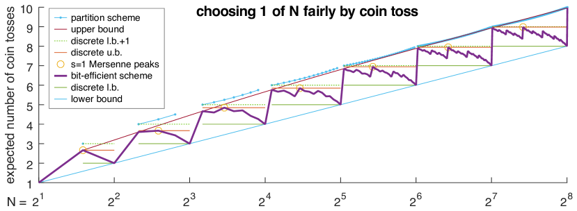
Figure 4.1. $e[n]$ and bounding curves.

Viewed as a curve (see fig. 4.1), the $e[n]$ sequence exhibits a fractal sawtooth structure with $m$ peaks in the $m^{\text{th}}$ epoch ($2^{m-1}<n\leq 2^{m}$) that recur with additional detail in subsequent epochs. Since eqn. (3.2) is an exponentially weighted sum of residues, the $e[n]$ curve spikes whenever an increment in $n$ causes an early element of the residue sequence $c_{i}=2^{i}\bmod n$ to jump in value. I.e., at $n=11,$ residue 5 jumps from $2\equiv 2^{5}\pmod{10}$ to $10\equiv 2^{5}\pmod{11}$. The first $m$ residues are constant within each epoch; the remaining residues determine the jumps.

In this section we determine the locations of these jumps; in the next we determine the values of the associated peaks. Before giving the general formula, we give special attention to the first two series of peaks, which will later yield upper bounds on the whole sequence. The first series occurs at the beginning of the epoch:

Proposition 8 (Fermat peaks).

Residue term $c_{k}$ makes a maximal jump at Fermat number $n=F_{k}$, producing a peak.

Proof.

With $n=F_{k},$ the residue sequence $2^{i}\bmod n$ is $\{1,2,4,\cdots,2^{k-1},2^{k}=n-1,n-2,n-4,\cdots,n-2^{k-1}\}$ repeating, while the residue sequence for $2^{i}\bmod(n-1)$ is $\{1,2,4,\cdots,2^{k-1},0,0,0\cdots\}$ nonrepeating. Therefore the jump is $2^{k}-0=n-1$, the largest possible. ∎

The second series is associated with the second varying term in the residue sequence. Its evolution is most conveniently tracked every other epoch:

Proposition 9 (First Mersenne peaks).

In epoch $m=2k$, residue term $c_{2k+1}$ makes the second largest jump at $n=F_{2k+1}/3$.

Proof.

We show that $2\equiv 2^{2k+1}\pmod{n-1}$ and $n-1\equiv 2^{2k+1}\pmod{n}$. Useful facts are A: $3\mid M_{2k},\,k>0$ because $M_{2k}=M_{k}F_{k}=M_{k}(M_{k}+2)$; B: $1\equiv a\pmod{b}$ and $c|b$ $\implies$$1\equiv a\pmod{b/c}$; C: $1\equiv a\pmod{b}$$\implies$$2\equiv 2a\pmod{2b}$; D: $n-1=(F_{2k+1}-3)/3=(2M_{2k}-2)/3=\nicefrac{{2}}{{3}}M_{2k}$; E: $3\mid F_{2k+1},k\geq 0$ because $3\mid M_{2k}$ and $F_{2k+1}=2M_{2k}+3$. First, $1\equiv(M_{2k}+1)\pmod{M_{2k}}$ $\stackrel{{\scriptstyle A,B}}{{\implies}}$ $1\equiv 2^{2k}\pmod{M_{2k}/3}$ $\stackrel{{\scriptstyle C}}{{\implies}}$ $2\equiv 2\cdot 2^{2k}\pmod{2M_{2k}/3}\stackrel{{\scriptstyle D}}{{=}}2^{2k+1}\pmod{n-1}$. Second, $n-1\equiv 3n-1\pmod{n}$ $\implies$ $n-1\equiv 2^{2k+1}\pmod{n}$ because $3n-1=3(F_{2k+1}/3)-1\stackrel{{\scriptstyle\text{E}}}{{=}}2^{2k+1}$. Finally, note that the jump $n-3$ is second largest because $n-1$ is the maximal residue value and $2$ is the minimal value that can occur in a (repeating) residue class after the first position. ∎

The remaining series of peaks are associated with smaller jumps:

Proposition 10 (All Mersenne peaks).

Residue $c_{m+s}$ jumps $n-F_{s}$ to peak value $n-1$ in epoch $m=2sk$ at

$$n=N_{s}[k]\doteq F_{s(2k+1)}/F_{s}$$

Proof.

We claim that at $n=F_{s(2k+1)}/F_{s}\in\mathbb{N}$, $2^{s}\equiv 2^{s(2k+1)}\pmod{n-1}$, and $n-1\equiv 2^{s(2k+1)}\pmod{n}$, yielding a jump of $n-1-2^{s}=n-F_{s}$. Useful facts are A: $F_{s}\mid F_{s(2k+1)}$ because $(a-b)\mid(a^{q}-b^{q})$, choose $a=2^{s},b=-1,q=2k+1$; B $M_{2sk}=(2^{2sk}-1)=(2^{sk}-1)(2^{sk}+1)=M_{sk}F_{sk}$; C: $1\equiv a\pmod{b}$$\implies$$2^{s}\equiv 2^{s}a\pmod{2^{s}b}$; D: $n-1=(F_{s(2k+1)}-F_{s})/F_{s}=2^{s}(M_{ks}F_{ks})$. Fact A settles claim 1, that $n\in\mathbb{N}$. For claim 2, $1\equiv(M_{2sk}+1)\pmod{M_{2sk}}$ $\stackrel{{\scriptstyle B}}{{\implies}}$ $1\equiv 2^{2sk}\pmod{M_{sk}F_{sk}}$ $\stackrel{{\scriptstyle C}}{{\implies}}$ $2^{s}\equiv 2^{s}\cdot 2^{2sk}\pmod{2^{s}\cdot M_{sk}F_{sk}}\stackrel{{\scriptstyle D}}{{=}}2^{s(2k+1)}\pmod{n-1}$. For claim 3, $n-1\equiv F_{s}n-1\pmod{n}$ $\implies$ $n-1\equiv 2^{s(2k+1)}\pmod{n}$ because $F_{s}n-1=F_{s}(F_{s(2k+1)}/F_{s})-1\stackrel{{\scriptstyle\text{A}}}{{=}}2^{s(2k+1)}$. ∎

To locate the peaks in the epochs between $2sk$ and $2s(k+1)$, it is convenient to note that because the moduli $n$, $2n$, and $(2n-1)$ all generate similar residue sequences for the generator $2^{i}$, each peak is echoed in subsequent epochs. In particular, from $N_{s}[k]$, the $s^{\text{th}}$ peak propagates up through the epochs via $s$ iterations of $n\to 2n$ alternating with $s$ iterations of $n\to 2n-1$. E.g., the $s=2$ peaks occur at $n={\bf 1},{\scriptstyle\times 2=}2,{\scriptstyle\times 2=}4,{\scriptstyle\times 2-1=}7,{\scriptstyle\times 2-1=}{\bf 13},26,52,103,{\bf 205},410,820,\cdots$ with the bolded entries being $N_{2}[k]$ for $k=0,1,2,\cdots$. We call these the Mersenne peaks because the peak at $n=N_{s}(1)$ in epoch $s$ is anticipated by a bump at Mersenne number $n=M_{s}$ in epoch $s-1$ under the progression $n\to 2n-1$, i.e., $N_{s}(1)=2M_{s}-1$.

5. Peak values

By unrolling the recursive fixpoint at Mersenne peaks $n=N_{s}[k]$ and solving recurrences it is possible to get a closed-form solution for selected $e[n]$. Defining $J_{s}[j]\doteq sj2^{sj}/F_{sj}$, the $k^{\text{th}}$ instance of the $s^{\text{th}}$ peak has location and value

(5.1) $$\begin{array}[]{rcl}e\left[n=N_{s}[k]=F_{s(2k+1)}/F_{s}\right]&=&J_{s}[2k+1]-J_{s}[1]+2/F_{s}\\ &=&\frac{s(2k+1)2^{s(2k+1)}}{F_{s(2k+1)}}-\frac{s2^{s}}{F_{s}}+\frac{2}{F_{s}}\\ &=&2sk+\frac{s+2}{F_{s}}-\frac{s(2k+1)}{F_{s(2k+1)}}\end{array}$$

6. Bounds on $e[n]$

We begin by summarizing the results of this section: For $m=\lceil\log_{2}n\rceil$ and $j=m+1+(m\bmod 2)$, we have the bounds

$$\begin{array}[]{rrclclcl}\text{discrete:}&m&\leq&e[n]&\leq&2+e[F_{j}/3]+m-j&<&m+1\\ \text{continuous:}&\log_{2}n&\leq&e[n]&\leq&2+\nicefrac{{(n-1)}}{{n}}\log_{2}(n-1)&<&2+\log_{2}n\,,\end{array}$$

with all $\leq$ bounds sharp. Fig. (4.1) depicts all these relationships.

The lower bounds are trivial. We begin with the loose discrete upper bound. Regarding eqn. (5.1), note that the first term, $2sk$, is the number of the epoch in which the peak appears. The second term attains a maximum value of 1 at $s=1,$ and the third term always reduces the sum. Consequently 2sk+1 upper-bound all peaks in the epoch or, equivalently,

Proposition 11.

$e[n]<\lceil\log_{2}n\rceil+1$.

6.1. Continuous upper bound

The largest spikes in the $e[n]$ sequence occur at the Fermat numbers $n=F_{m}$, because these are associated with the largest jumps in the residue sequence, and these jumps occur earliest in the exponentially decaying sum for $e[n]$ in eqn. 3.2. Consequently we can construct an upper bound for the whole curve from the Fermat peak values:

Proposition 12 (Fermat bound).

For all $n$ in the $m^{\text{th}}$ epoch, $e[n]\leq 2+\frac{n-1}{n}\log_{2}(n-1)<2+\log_{2}n$ with equality at $n=F_{m}$.

Proof.

To obtain $e[n=F_{m}]$, we unroll the recurrence in algorithm (1) and observe that for Fermat numbers, the sequence $z[m]=2ng/(f-h)$ has recurrence $z[m]=2z[m-1]+M_{m-1}$, $z[1]=4$, whose solution $z[m]=m2^{m-1}+2^{m}+1$ implies that $g/(f+h)=z[m]/(2n)=2+m2^{m}/F_{m}=2+J_{1}[m]$ at $n=F_{m}$. Substituting in $m=\log_{2}(n-1)$ gives $e[n=F_{m}]=2+\nicefrac{{1}}{{n}}(n-1)\log_{2}(n-1)$. To establish the upper bound, note that any other peak located at $N_{s}[k]$ in the same epoch (satisfying $m=2sk$) has the loose upper bound $e[N_{s}[k]]<2sk+1=m+1=\lfloor\log_{2}(n-1)\rfloor+2$ for any $n>F_{m}$ in the $m^{\text{th}}$ epoch. Thus we need to show that $\lfloor\log_{2}(n-1)\rfloor+2<2+\frac{n-1}{n}\log_{2}(n-1)$ at any non-Fermat peak. In any epoch, the lhs is constant and rhs is increasing, so it suffices to show that it holds at the first non-Fermat peak, which occurs at $n=N_{1}[k]=F_{2k+1}/3,k>1$. There we have $\frac{n-1}{n}=1-3/F_{2k+1}$; choose worst case $k=2$. Then lhs is 5 and rhs is $2+(1-3/F_{5})\log_{2}(F_{5}/3-1)=2+(10/11)\log_{2}10>5$. ∎

6.2. Discrete upper bound

Since early residues have exponentially larger weights in the expectation, peaks from the $s=1$ Mersenne peaks dominate all others. This can be expressed as a "stair-step" curve that gives a constant (but sharp) upper bound for each epoch:

Proposition 13 (Mersenne bound).

Let $j=2k+1$ for $k\in\mathbb{N}$. Then $e[n]\leq e[F_{j}/3]=j2^{j}/F_{j}$ for all $n$ in epoch $m=j-2$ and $e[n]\leq 1+e[F_{j}/3]$ for all $n$ in epoch $m=j-1$.

Proof.

The odd $m$ case is simply the value $e[n]$ at peak $n=N_{1}(k)$ from eqn. 5.1, line 2. The even case follows from $e[2n]=e[n]+1$ and the peak propagation rule. To show that this also upper-bounds the Fermat peaks, we need $e[n]=2+\frac{n-1}{n}\log_{2}(n-1)<j2^{j}/F_{j}$ at Fermat peak locations $n=F_{j-2}$. Putting all in terms of $k=(j-1)/2$ and taking rhs-lhs yields $\frac{4^{k}(6k-5)-4}{2F_{2k-1}F_{2k+1}}$, which is zero at $k=1$ and positive for $k>1$. ∎

7. Orderings

We close with result on fair orderings: It is more toss-efficient to determine an ordering of $k$ objects by choosing 1 of $k!$, than by sequentially choosing 1 of $k$, then 1 of $k-1,$ etc. Specifically,

Proposition 14 (Logarithmic subadditivity).

$\forall_{a,b}\>e[ab]\leq e[a]+e[b]$ .

Proof.

We prove $\forall_{a,b}\ngtr$, $\exists_{a,b}=$, $\exists_{a,b}<$. Claim 1: By prop. , $e[n]$ is toss-efficient. No toss-efficient procedure can have $\exists_{a,b}\>e[ab]>e[a]+e[b]$ because one could then reduce $e[ab]$ by simply choosing 1 of $a$ and then 1 of $b$. Claim 2: Since $e[2n]=1+e[n]$, we have equality $e[ab]=e[a]+e[b]$ when $a$ or $b$ is a power of 2. Claim 3: Consider a Fermat peak at $a=F_{s}$ and a Mersenne peak at $b=F_{s(2k+1)}/F_{s}$ (see prop. 10). Using the peak-value formulas from prop. 12 and eqn. 5.1 we obtain $e[a]+e[b]-e[ab]=e[F_{s}]+e[F_{s(2k+1)}/F_{s}]-e[F_{s(2k+1)}]=2/F_{s}$. ∎

We further conjecture that the inequality is strict whenever $a$ and $b$ both have odd factors.

Appendix A Lucky numbers and how to find them

The pattern of lucky numbers in a finite lottery will depend on the mapping from random flips to ticket numbers. The common programming idiom

$$\text{randomInteger}(n):=\text{randomInteger}(2^{b})\bmod n$$

assigns more random outcomes to lower ticket numbers, whereas

$$\text{randomInteger}(n):=\lfloor n\cdot{\tt randomFloat}[0,1)\rfloor\>,$$

widely enshrined in the libraries of scientific computing environments, has patterned lucky numbers, exemplifed by

Proposition 15.

Given $b$, choose any $n=2^{a}M_{k}$ with $a\geq 0$, $k>1$, $a+k\leq b$, and let $p\sim\mathcal{U}_{b}(1)$ be a random variable uniformly sampled from the set $U_{b}\doteq\{0,\nicefrac{{1}}{{2^{b}}},\nicefrac{{2}}{{2^{b}}},\nicefrac{{3}}{{2^{b}}},\cdots,\nicefrac{{2^{b}-2}}{{2^{b}}},\nicefrac{{2^{b}-1}}{{2^{b}}}\}$. Then random integers $q\doteq\lfloor np\rfloor\in\{0,\cdots,n-1\}$ and $q\bmod M_{k}$ are both nonuniformly distributed with a length-$M_{k}$ pattern of lucky and unlucky numbers. Furthermore, if $k\mid$$b-a$, then given two numbers $0\leq q_{L},q_{U}<n$ with $M_{k}-1\equiv q_{L}\pmod{M_{k}}$ and $M_{k}-1\not\equiv q_{U}\pmod{M_{k}}$, $q_{L}$ is lucky with $\frac{Pr(q=q_{L})}{Pr(q=q_{U})}=$$\frac{c+1}{c}$ with $c=\lfloor\frac{2^{b-a}}{M_{k}}\rfloor\in\mathbb{N}$ as small as $c=1$ for $n=3\cdot 2^{b-2}$.

Proof.

$\lfloor np\rfloor\pmod{M_{k}}$ wraps $U_{b}$, viewed as a knotted string, around a cylinder of circumference $M_{k}$ with $M_{k}$ equidistant notches, then assigns each knot to the closest notch in one direction. Since $2^{a}\mid 2^{b}$, the string wraps exactly $2^{a}$ times such that each consecutive group of $2^{b-a}$ samples from $U_{b}$ is identically assigned to elements of the residue set $\{0,\cdots,M_{k}-1\}$. Since $2^{b-a}>M_{k}$ and $M_{k}\nmid 2^{b-a}$, by the pigeonhole principle, $2^{b-a}\bmod M_{k}$ elements of the residue set get assigned one extra sample. If $k\mid b-a$, exactly $1\equiv 2^{b-a}\pmod{M_{k}}$ element gets this surplus, because $(x-y)\mid(x^{z}-y^{z})$ and thus $k\mid b-a$$\implies$($2^{k}-1)\mid(2^{k(b-a)/k}-1)$$\implies$$M_{k}\mid M_{b-a}$$\implies$$1\equiv 2^{b-a}\pmod{M_{k}}$. The lucky element’s position in the residue set is: last for $\lfloor np\rfloor$; first for $\lceil np\rceil;$ middle for $\lfloor np\rceil$. The remainder of the proposition follows from arithmetic. ∎

In practice, the pattern and prominence of lucky numbers will also depend on the number of bits used internally for CPU arithmetic and the choice of rounding scheme. At time of writing the bias can be demonstrated in several numerically sophisticated programming environments, even when $M_{k}$ is replaced by an arbitrary odd number. For example, with $b=53$ bits in the IEEE754 double-precision floating point significand, let $j$ be a small integer, $f=F_{j}$, and $n=\lfloor 2^{b-1}(F_{j}/F_{j-1})\rceil$. Then in $k$ trials, lottery ticket numbers $\pmod{f}$ are winners in Matlab or Octave with non-uniform relative frequencies

$$\mathtt{full(sparse(1+mod(randi(n,k,1),f),1,1,f,1))/k}$$

Similar bias can be elicited from the ${\tt sample}()$ and ${\tt runif}$() functions in the R statistics environment. Python and Mathematica use arbitrary-precision arithmetic which drives the bias down to insignificant levels.

Rejection sampling offers a trivial but inefficient way to restore fairness: Obtain a fair $R\in\{1,\ldots,2^{b}\}$ from a round of $b$ tosses, reject and repeat if $R>n$. Naïvely this takes a impractical $e^{\prime}=1+(1-n/2^{b})e^{\prime}=2^{b}/n$ rounds of $b$ tosses each. But if we instead reject when $R>n\lfloor 2^{b}/n\rfloor$, the largest multiple of $n$ that is $\leq 2^{b}$, then $R\bmod n$ is a fair draw from $\{0,\ldots,n-1\}$ and the expectation falls to $e^{\prime}=1/(1-(2^{b}\bmod n)/2^{b})$ rounds. In tosses, $b\leq e<2b$, $e[3]=b$ and $e[F_{b-1}]=2b(1-1/F_{b})$. Although quite bit-inefficient, C++ libraries appear to use an (algebraically) equivalent strategy.

Appendix B Solution for $e[n]$ recurrence in (3.1)

Algorithm 1 An integer-arithmetic solution of the recursive fixpoint for $e[n]$. $m$ is the number of coin flips in each round; $o$ is the number of possible outcomes; $r$ is the number of unassigned outcomes; and $r/o$ is the probability of going another round.

Input: Odd $n\geq 3$.

Initialize:

$f\leftarrow 1,\>g\leftarrow 0,\>h\leftarrow 1,\>r\leftarrow 1.$

Iterate:

$m,o\leftarrow\min_{m}\text{s.t. }o=2^{m}r>n$,
      $r\leftarrow o-n$,  $f\leftarrow fo$,  $g\leftarrow(g+mh)o$,  $h\leftarrow hr$.

Until:

$r=1$.

Output: $e[n]=g/(f-h)$.

References

- [1] Jacques Bernard and Gérard Letac, Construction d’évenements équiprabables et coefficients multinomiaux modulo , Illinois Journal of Math 17 (1973), 317–332.
- [2] H. G. Bissinger, Friday night lights: A town, a team, and a dream, Addison-Wesley, 1990.
- [3] Meyer Dwass, Unbiased coin tossing with discrete random variables, Annals of Mathematical Statistics 43 (1972), no. 3, 860–864.
- [4] Dexter Kozen, Optimal coin flipping, Panangaden Festschrift (Switzerland) (F. van Breugel et al., ed.), LNCS, vol. 8464, Springer, 2014, pp. 407–426.
- [5] Quentin F. Stout and Bette Warren, Tree algorithms for coin tossing with a biased coin, Annals of Probability 12 (1984), no. 1, 212–220.
- [6] John von Neumann, Various techniques used in connection with random digits, Tech. Report 12, U.S. National Bureau of Standards, 1951, To unbias a coin, wait for 2 different outcomes, keep 1st.