Isoperimetric inequalities for eigenvalues of the Laplacian on cycles with fixed resistance metric

Abstract

For cycles with non-negative weights on its edges, we define its global resistance as the sum of the distances given by the effective resistance metric between adjacent vertices. We prove the following result: for the Laplace operator on the 3-cycle with global resistance equal to a given constant, the maximal value of the smallest positive eigenvalue and the minimal value of the largest eigenvalue, are both attained if and only if all the weights are equal to each other.

Keywords— Graph Laplacians, eigenvalues, extremal problems, resistance metric, isoperimetric inequalities

1 Introduction

The study of isoperimetric inequalities for eigenvalues of the Laplacian and more general elliptic operators has a long history (see, for example [10, 3, 6]). Back in the 1920’s, Georg Faber and Edgar Krahn proved independently of each other, a conjecture stated decades earlier by John W.S. Rayleigh. This conjecture established that, among all the planar domains with fixed area, the circle is the one with least first Dirichlet eigenvalue. That result, known as the Faber–Krahn inequality, is usually regarded as a starting point and a cornerstone of this theory.

For eigenvalues of graph Laplacians, the study of isoperimetric inequalities is much more recent than the one for Laplacians on manifolds. In [5], J. Friedman introduced the concept of the boundary of a graph and considered Faber–Krahn type problems for the eigenvalues of the Laplacian for regular trees. Different isoperimetric problems for eigenvalues in that context have been studied by various authors such as [9, 1, 2, 7]. In those works, the aim is to find the graph for which the Laplacian eigenvalues are extremal when some chosen volume of the graph (say, its number of vertices or edges) is fixed. Minimizers of the first eigenvalue have been found for several classes of graphs. Just to mention one of these results, among other similar results, in [1] it is shown that, within the class of trees with fixed number of interior and boundary vertices, the minimal Dirichlet eigenvalue is attained for a comet (a star-shaped graph with a long tail), for which the boundary is the set of vertices with degree 1. That minimizer is unique up to isomorphism.

The present work is somewhat different to those referred in the previous paragraph in a couple of aspects. First, we consider graphs without boundary. Second, here the graphs considered are held fixed, and what varies are the weights on its edges. More precisely, we look at the eigenvalues of the usual Laplace operator on cycles, and the geometric quantity to be fixed (the global resistance presented in definition 2) is one that depends on the weights. This quantity is defined in terms of a metric of the graph known as the effective resistance metric (or just resistance metric) that was defined in [4] and originally inspired by electrical network theory. The effective resistance metric plays a key role in Jun Kigami’s construction of the Laplacian on self-similar fractals, and for the construction of a natural metric on those fractal sets (see [8, 11]).

Our work is organized as follows. In section 2 we present the resistance metric and introduce notation. In section 3 we define the global resistance and make some calculations in this regard. The main result of this work concerns the 3-cycle and is given in theorem 1. It establishes that once the global resistance is fixed, the smallest positive eigenvalue of the Laplacian is maximized and the largest eigenvalue is minimized when the weights on the edges are all equal. The proof of this theorem is contained in section 4. In section 5 we comment briefly on the plausible generalization of this result to larger $n$-cycles.

2 The Effective Resistance Metric

In this section we introduce notation and recall some basic definitions and well known facts from the analysis of graph Laplacians.

Let $\Gamma$ be a finite, simple and undirected graph with no loops. Denote by $\{v_{0},\dots,v_{n-1}\}$ the vertices of $\Gamma$. Given a pair of vertices $v_{i}$ and $v_{j}$ connected to each other, we will write $v_{i}\sim v_{j}$. For such a pair, $c_{i,j}>0$ will denote the weight on the edge between them and, following a well known electrical network analogy (originally introduced in [4]), we will call the $c_{i,j}$ the conductances of the graph.

It is convenient to define $c_{i,j}=0$ whenever the vertices $v_{i}$ and $v_{j}$ are not connected by an edge. In particular, the no loops condition means that $c_{i,i}=0$. We denote by $\ell(\Gamma)$ the set of real-valued functions defined on the vertices, and for $f\in\ell(\Gamma)$ we consider the usual norm and inner product. That is,

$$\|f\|^{2}=f(v_{0})^{2}+\cdots+f(v_{n-1})^{2},\qquad{\big{\langle}f,g\big{\rangle}}=f(v_{0})g(v_{0})+\cdots+f(v_{n-1})g(v_{n-1}).$$

The Laplacian on $\Gamma$ is the linear operator on $\ell(\Gamma)$ given by

$$(\Delta f)(v_{k})=\sum_{j=0}^{n-1}c_{j,k}(f(v_{k})-f(v_{j})).$$

It is well known that $\Delta$ is a non-negative operator, so that in particular it is self-adjoint. The associated quadratic form $E(f,g)={\big{\langle}\Delta f,g\big{\rangle}}$ is known as the energy of the graph. The expression $E(f)=E(f,f)$ defines a norm on the $n-1$ dimensional subspace of $\ell(\Gamma)$ that is orthogonal to the space of constant functions. This energy norm can also be written in the form

$$E(f)=\sum_{i\leq j}c_{i,j}(f(v_{i})-f(v_{j}))^{2}.$$ (1)

The resistance metric between vertices of a weighted graph is defined in terms of the energy, as follows.

Definition 1.

Let $v_{i}$ and $v_{j}$ be two vertices in a weighted graph $\Gamma$.

$$m =\min\left\{E(f)\ |\ f(v_{i})=1,f(v_{j})=0\right\}.$$ (2)

(3)

$$d_{\rm r}(v_{i},v_{j}) =\frac{1}{m}.$$

The expression $d_{\rm r}(\cdot,\cdot)$ is called the effective resistance metric.

We refer to [8, 11] for the proof that the effective resistance metric is indeed a metric.

It is known that the minimum in (2) is attained by the so-called harmonic extension. That is, the unique function such that $f(v_{i})=1$, $f(v_{j})=0$ and $(\Delta f)(v_{k})=0$ for all $k\geq 2$ (see e.g. Theorem 2.1.6 in [8] for a proof and more details of this). This provides us with a formulation of the effective resistance metric that is computationally convenient:

Let’s consider the distance between the first two vertices, namely $d_{\rm r}(v_{0},v_{1})$. This implies no loss of generality, since we can re-label the vertices as needed. The function $f$ with mininal energy $E(f)$ is the corresponding harmonic extension of $f(v_{0})=1$ and $f(v_{1})=0$ , and it satisfies $(\Delta f)(v_{k})=0$ for all $k\geq 2$. Let $H$ be the matrix representation of $\Delta$ with trespect to the canonical basis $\{e_{0},\dots,e_{n-1}\}$ (where $e_{j}(v_{k})=\delta_{j,k}$).

Consider the decomposition

$$H=\begin{pmatrix}M&J^{t}\cr J&L\end{pmatrix},\qquad\qquad M=\begin{pmatrix}\sum_{k}c_{0,k}&-c_{0,1}\cr-c_{0,1}&\sum_{k}c_{1,k}\end{pmatrix}.$$

Let $f$ be the corresponding harmonic extension and split it as

$$f=\begin{pmatrix}f_{0}\cr f_{1}\end{pmatrix}\qquad f_{0}=\begin{pmatrix}1\cr 0\end{pmatrix}\qquad f_{1}=\begin{pmatrix}f(v_{2})\cr\vdots\cr f(v_{n-1})\end{pmatrix}$$

The condition $(\Delta f)(v_{k})=0$ gives $Jf_{0}+Lf_{1}=0$ so that $f_{1}$ is determined by $f_{1}=-L^{-1}Jf_{0}$. This in turn, gives an explicit formula for the minimal value of the energy (and hence for the metric $d_{\rm r}(v_{0},v_{1})$) as

$$E(f_{0}) ={\big{\langle}(M-J^{t}L^{-1}J)f_{0},f_{0}\big{\rangle}}.$$ (4)

$$d_{\rm r}(v_{0},v_{1}) =1/E(f_{0}).$$

We note that if we multiply all the conductances by a constant $\alpha$, then $M-J^{t}L^{-1}J$ (and therefore $E(f_{0})$ as well) is multiplied by the same constant. The resistance metric is then inversely proportional to $\alpha$.

3 Global Resistance in Cycles

In this section we introduce the global resistance. This will be the geometric quantity to be fixed in the isoperimetric problems to be considered in section 4.

Definition 2.

For a weighted graph $\Gamma$ define the global resistance $\rho(\Gamma)$ by

$$\rho(\Gamma)=\sum_{v_{i}\sim v_{j}}d_{\rm r}(v_{i},v_{j})$$

where the sum is taken over all un-ordered pairs of adjacent vertices.

To avoid any possible confussion, we remark that even though the effective resistance metric is defined for any pair of vertices in the graph, in the definition of the global resistance we only consider adjacent pairs.

For the 3-cycle, the operators in (4) are given by

$$M=\begin{pmatrix}c_{0,1}+c_{0,2}&-c_{0,1}\cr-c_{0,1}&c_{0,1}+c_{1,2}\end{pmatrix},\qquad J=\begin{pmatrix}-c_{0,2}&-c_{1,2}\end{pmatrix},\qquad L=\Bigl{(}c_{0,2}+c_{1,2}\Bigr{)}$$

From this, the metric can be easily calculated to be

$$d_{\rm r}(v_{0},v_{1})=\frac{c_{0,2}+c_{1,2}}{c_{0,1}c_{0,2}+c_{0,1}c_{1,2}+c_{0,2}c_{1,2}}$$

By symmetry we can see that

$$d_{\rm r}(v_{0},v_{2})=\frac{c_{0,1}+c_{1,2}}{c_{0,1}c_{0,2}+c_{0,1}c_{1,2}+c_{0,2}c_{1,2}}$$

and

$$d_{\rm r}(v_{1},v_{2})=\frac{c_{0,1}+c_{0,2}}{c_{0,1}c_{0,2}+c_{0,1}c_{1,2}+c_{0,2}c_{1,2}}.$$

The global resistance of the 3-cycle then becomes

$$\rho(T)=\frac{2(c_{0,1}+c_{0,2}+c_{1,2})}{c_{0,1}c_{0,2}+c_{0,1}c_{1,2}+c_{0,2}c_{1,2}}$$ (5)

Note that if we hold fixed two of the conductances, then $\rho(T)$ is decreasing with respect to the third conductance. This simple observation will be useful later.

4 Isoperimetric Inequalities for 3-Cycles

In this section we will prove our main result, namely:

Theorem 1.

Let $\lambda_{1}\leq\lambda_{2}$ be the positive eigenvalues of the Laplace operator associated with a weighted 3-cycle $T$. Then the following inequalities hold:

$$\lambda_{1}\rho(T)\leq 6\leq\lambda_{2}\rho(T).$$

In each of both sides, the equality occurs if and only if the weights are all equal to each other.

The proof will follow from three lemmas, which might be interesting on their own right, as they show that the eigenvalues depend on the conductances in a nice and simple way, as soon as the global resistance is fixed. The first of these lemmas, deals with the case where two of the conductances are equal to some constant $b$. In this case, there is the notable and rather surprising property that, even though the eigenvalues vary, the corresponding eigenvectors stay the same. Indeed, for the case where all the conductances are equal to $1$, we have that $\lambda=3$ is an eigenvalue with $\{(1,-1,0),(1,1,-2)\}$ an orthogonal basis of its eigenspace; those vectors will also be eigenvectors for any choice of $b$. More precisely:

Lemma 1.

Let $T$ be a 3-cycle with two conductances equal to some $b>0$ and global resistance $\rho(T)=2.$

1. If $b\geq 1$ and $b=c_{0,2}=c_{1,2}$, then $\{(1,1,1),(1,-1,0),(1,1,-2)\}$ are eigenvectors corresponding to the (ordered) eigenvalues $0=\lambda_{0}<\lambda_{1}\leq\lambda_{2}$.

2. If $b\leq 1$ and $b=c_{0,2}=c_{1,2}$, then the order of the above eigenvectors for $\lambda_{1}$ and $\lambda_{2}$ is reversed, with $(1,1,-2)$ being eigenvalue for $\lambda_{1}$, and $(1,-1,0)$ eigenvalue for $\lambda_{2}$.

3. Let $T$ be a 3-cycle for either of the above situations and any value of $b$. The eigenvalues of $T$ satisfy

   $$\lambda_{1}\leq 3\leq\lambda_{2}$$

   with equality if and only if all the conductances are equal to $1$.

Proof.

Substitution of $b=c_{0,2}=c_{1,2}$ in (5) yields

$$c_{0,1}=\frac{b(2-b)}{2b-1}.$$

so that the positivity condition for the conductance restricts the possible values of $b$ to the interval $(1/2,2]$.

The Laplacian matrix is in this case

$$H=\begin{pmatrix}\displaystyle{\frac{b(b+1)}{2b-1}}&\displaystyle{-\frac{b(2-b)}{2b-1}}&-b\cr\ &\ &\ \cr\displaystyle{-\frac{b(2-b)}{2b-1}}&\displaystyle{\frac{b(b+1)}{2b-1}}&-b\cr\ &\ &\ \cr-b&-b&2b\end{pmatrix}$$

Direct computation shows that

$$H\begin{pmatrix}\phantom{-}1\cr-1\cr\phantom{-}0\end{pmatrix}=\frac{3b}{2b-1}\begin{pmatrix}\phantom{-}1\cr-1\cr\phantom{-}0\end{pmatrix}\qquad{\rm and}\qquad H\begin{pmatrix}\phantom{-}1\cr\phantom{-}1\cr-2\end{pmatrix}=3b\begin{pmatrix}\phantom{-}1\cr\phantom{-}1\cr-2\end{pmatrix}.$$

Since $3b/(2b-1)\leq 3b$ if and only if $b\geq 1$, then $\lambda_{1}=3b/(2b-1)$ for $b\leq 1$ and $\lambda_{1}=3b$ for $b\geq 1$. So, $\lambda_{1}$ is increasing as a function of $b\in(1/2,1]$ and decreasing for $b\geq 1$ and we can see that its maximum value is attained at $b=1$. The assertion for $\lambda_{2}$ follows in just the same way. ∎

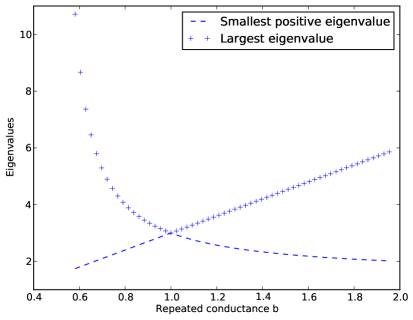
Figure 1: The two positive eigenvalues of the Laplacian of a 3-cycle conductances $\{b,b,(b(2-b))/(2b-1)\}$.

The behaviour of the eigenvalues in the previous lemma is shown in figure 1.

The next lemma establishes that when the middle value of the conductances is held fixed, we can make the maximal eigenvalue $\lambda_{2}$ smaller by approaching one of the other two conductances to that middle value.

Lemma 2.

Let $T$ be a weighted 3-cycle with vertices $\{v_{0},v_{1},v_{2}\}$, global resistance $\rho(T)=2$, and denote by $c_{i,j}$ the conductance on the edge joining $v_{i}$ with $v_{j}$.

1. Supposse that

   $$c_{0,1}<1\leq c_{0,2}\leq c_{1,2}=r.$$

   and fix $c_{0,2}=b$ for some $b\geq 1$. Let $\lambda_{2}(r)$ be the largest eigenvalue of the Laplacian associated with $T$. Then $\lambda_{2}(r)$ is an increasing function of $r\geq b$.

2. Supposse that

   $$r=c_{1,2}\leq c_{0,2}\leq 1<c_{0,1}.$$

   and fix $c_{0,2}=b\leq 1.$ Then, $\lambda_{2}(r)$ is a decreasing function of $r\leq b$.

Proof.

First, we give a characterization for the eigenvector associated with $\lambda_{2}$, for conductances satisfying $c_{0,1}\leq c_{0,2}\leq c_{1,2}$ and being otherwise arbitrary. For a function $u\in\ell(T)$ given by $u(v_{j})=x_{j}$, the energy (1) takes the form

$$E((x_{0},x_{1},x_{2}))=c_{0,1}(x_{0}-x_{1})^{2}+c_{0,2}(x_{0}-x_{2})^{2}+c_{1,2}(x_{1}-x_{2})^{2}.$$ (6)

The Schwarz quotient

$$S(u)=\frac{E(u)}{\|u\|^{2}}$$ (7)

reaches its maximum value exactly for the functions $u$ such that $\Delta u=\lambda_{2}u$. Note that for any permutation of the triad $(x_{0},x_{1},x_{2})$ the denominator in (7) does not change, while the energy will be maximal when the largest distance $|x_{i}-x_{j}|$ is next to the largest conductances and the smallest distance $|x_{i}-x_{j}|$ is next to the smallest conductances. Therefore a necessary condition for $\Delta u=\lambda_{2}u$ is that

$$|x_{0}-x_{1}|\leq|x_{0}-x_{2}|\leq|x_{1}-x_{2}|$$

From the orthogonality condition $x_{0}+x_{1}+x_{2}=0$, we can see that the term with largest absolute value must have different sign than the other two, so that it must be involved in the two largest distances. So, we obtain the necessary condition $|x_{0}|\leq|x_{1}|\leq|x_{2}|$ for $(x_{0},x_{1},x_{2})$ being an eigenvector with eigenvalue $\lambda_{2}$.

Without loss of generality, we can always chose the eigenvector to be such that

$$x_{2}<0<x_{0}\leq x_{1}<|x_{2}|=x_{0}+x_{1}\qquad{\rm and}\qquad x_{0}^{2}+x_{1}^{2}+x_{2}^{2}=1.$$ (8)

For $b>1$ a given constant, the condition $\rho(T)=2$ determines $c_{0,1}$ as a function of the variable $r$.

Precisely,

$$c_{0,1}=\frac{r(b-1)-b}{1-b-r}.$$

Now, we suppose that $u(v_{j})=x_{j}$ is an eigenvector of $\Delta_{r_{0}}$ for some fixed $r_{0}>a$, with eigenvalue $\lambda_{2}(r_{0})$. Assume also that $(x_{0},x_{1},x_{2})$ satisfies the conditions (8).

We want to show that

$$\lambda_{2}(r_{0})\leq\lambda_{2}(r_{1}).$$ (9)

whenever or $1\leq b\leq r_{1}\leq r_{0}$.

Note that

$$\lambda_{2}(r_{0}) =E_{r_{0}}((x_{0},x_{1},x_{2}))$$

$$=\frac{r_{0}(b-1)-b}{1-b-r_{0}}(x_{0}-x_{1})^{2}+b(x_{0}-x_{2})^{2}+r_{0}(x_{1}-x_{2})^{2}$$

$$\lambda_{2}(r_{1}) \geq E_{r_{1}}((x_{0},x_{1},x_{2}))$$

$$=\frac{r_{1}(b-1)-b}{1-b-r_{1}}(x_{0}-x_{1})^{2}+b(x_{0}-x_{2})^{2}+r_{1}(x_{1}-x_{2})^{2}.$$

Hence, in order to obtain (9) it suffices to verify that

$$\frac{r_{0}(b-1)-b}{1-b-r_{0}}(x_{0}-x_{1})^{2}+r_{0}(x_{1}-x_{2})^{2}\leq\frac{r_{1}(b-1)-b}{1-b-r_{1}}(x_{0}-x_{1})^{2}+r_{1}(x_{1}-x_{2})^{2}.$$

To see this, we will show that

$$\gamma(r)=\frac{r(b-1)-b}{1-b-r}A+rB$$ (10)

is increasing for $r\geq b$, provided that $0<A\leq B$. Since by conditions (8) we have $(x_{0}-x_{1})^{2}\leq(x_{1}-x_{2})^{2}$ this would give the result.

Now,

$$\gamma^{\prime}(r) =\frac{(b-1+r)^{2}B-\left((b-1)^{2}+b\right)A}{(1-b-r)^{2}}$$

$$\geq\frac{(b-1+r)^{2}-\left((b-1)^{2}+b\right)}{(1-b-r)^{2}}A.$$

But

$$(b-1+r)^{2} \geq(2b-1)^{2}$$

$$=b^{2}+(b-1)^{2}+2b(b-1)$$

$$>(b-1)^{2}+b.$$

We conclude that $\gamma^{\prime}>0$ and (9) follows.

To prove part (2), first we observe that the change of order of the conductances means that the roles of $x_{2}$ and $x_{0}$ are interchanged, so that now we take the eigenvector for $\lambda_{2}$ to be such that

$$x_{0}<0<x_{2}\leq x_{1}<|x_{0}|=x_{1}+x_{2}\qquad{\rm and}\qquad x_{0}^{2}+x_{1}^{2}+x_{2}^{2}=1.$$ (11)

Take an eigenvector $(x_{0},x_{1},x_{0})$ with eigenvalue $\lambda_{2}$ for some $r_{0}\leq b\leq 1$, satisfying (11). For an arbitrary $r_{2}<r_{0}$ we want to show that $\lambda(r_{2})>\lambda(r_{0})$. Proceeding just like in part (1) it follows that it is enough prove the inequality

$$\frac{r_{0}(b-1)-b}{1-b-r_{0}}(x_{0}-x_{1})^{2}+r_{0}(x_{1}-x_{2})^{2}\leq\frac{r_{2}(b-1)-b}{1-b-r_{2}}(x_{0}-x_{1})^{2}+r_{2}(x_{1}-x_{2})^{2}.$$

Noting that $x_{0}=-x_{1}-x_{2}$ we can see that

$$(x_{0}-x_{1})^{2} =(2x_{1}-x_{2})^{2}$$

$$=((x_{1}-x_{2})+x_{1})^{2}$$

$$\geq 4(x_{1}-x_{2})^{2}.$$

In view of this, to get the inequality $\lambda(r_{2})>\lambda(r_{0})$ it is enough to verify that the function $\gamma(r)$ in (10) is decreasing whenever $A\geq 4B$. This is equivalent to the inequality

$$(b-1+r)^{2}B<4((b-1)^{2}+b)A.$$

It is clear that it is enough to check the extremal case $B=4A$ and $r=a$

$$(2b-1)^{2}<4((b-1)^{2}+b)$$

which can be easily verified. ∎

Figure 2: The two positive eigenvalues of the Laplacian of a 3-cycle with conductances equal to $\{(3-r)/(r+1),3/2,r\}$.

The analogous result for $\lambda_{1}$ is as follows. The ideas in the proof of lemma 3 are very similar to those of lemma 2, so we will not go into as much detail.

Lemma 3.

Let $T$ be a weighted 3-cycle with vertices $\{v_{0},v_{1},v_{2}\}$, global resistance $\rho(T)=2$, and denote by $c_{i,j}$ the conductance on the edge joining $v_{i}$ with $v_{j}$.

1. Supposse that

   $$c_{0,1}<1\leq c_{0,2}\leq c_{1,2}=r.$$

   and fix $c_{0,1}=b$ for some $b\geq 1$. Let $\lambda_{1}(r)$ be the largest eigenvalue of the Laplace operator associated with $T$. Then $\lambda_{1}(r)$ is a decreasing function for $r\geq b$.

2. Supposse that

   $$r=c_{1,2}\leq c_{0,2}\leq 1<c_{0,1}.$$

   and fix $c_{0,1}=b\leq 1.$ Then $\lambda_{1}(r)$ is increasing for $0<r\leq b$.

Proof.

If $u=(y_{0},y_{1},y_{2})$ is an eigenvector for $T$ corresponding to $\lambda_{1}$, then it minimizes de Schwarz quotient (7) among all the elements in $\ell(T)$ that are orthogonal to the constant functions. Opposite to the maximum, the minimal energy (6) will be attained when the largest of the $y_{j}$ is next to the smallest conductances, and the smallest $y_{j}$ is next to the largest conductances. Thus, for part 1, we can consider that

$$y_{0}<0<y_{2}\leq y_{1}<|y_{0}|=y_{1}+y_{2}\qquad{\rm and}\qquad y_{0}^{2}+y_{1}^{2}+y_{2}^{2}=1.$$ (12)

Proceeding as we did in the proof of lemma 2, proving that $\lambda_{1}(r)$ is decreasing for $r\geq b\geq 1$ reduces to verify that

$$\gamma(r)=\frac{r(b-1)-b}{1-b-r}(y_{0}-y_{1})^{2}+r(y_{1}-y_{2})^{2}$$

is decreasing. But, since $(y_{0}-y_{1})^{2}\geq 4(y_{1}-y_{2})^{2}$, we already have shown (in the last part of the proof of lemma 2) that such is the case.

For part 2 we can take the eigenvector $(y_{0},y_{1},y_{2})$ to satisfy the conditions (12). The fact that $\lambda_{1}(r)$ is increasing for $0<r\leq a\leq 1$ follows from

$$\gamma(r)=\frac{r(b-1)-b}{1-b-r}(y_{0}-y_{1})^{2}+r(y_{1}-y_{2})^{2}$$

being increasing, which is satisfied since $(y_{0}-y_{1})^{2}\leq(y_{1}-y_{2})^{2}$. ∎

See figures 2 and 3 for ilustrations of particular cases of lemmas 2 and 3.

Proof of theorem 1.

From the observation at the end of section 2 we have that $\rho(\alpha T)$ is inversely proportional to $\alpha$. Since the eigenvalues $\lambda_{j}$ are directely proportional to $\alpha$, we have that the products $\rho(\alpha T)\lambda_{j}$ do not change with $\alpha$. In other words, those products depend exclusively on the proportions between the conductances, not on their absolute values. So, without loss of generality, we can consider only the case when $\rho(T)=2$.

Given $T_{0}$ the 3-cycle with conductances equal to 1, we want to conclude that whenever $\rho(T)=2$ the inequalities

$$\lambda_{1}(T)\leq\lambda_{1}(T_{0})=\lambda_{2}(T_{0})\leq\lambda_{2}(T)$$ (13)

hold.

It is straightforward to verify that if we leave two of the conductances fixed, then $\rho(T)$ decreases as the third conductance increases. Therefore, in order to satisfy $\rho(T)=2$ it is necessary that, if $a<b<c$ are the conductances, we have either of the two situations

$$a \leq 1\leq b\leq c$$ (14)

$$a \leq b\leq 1\leq c.$$ (15)

Supposse that for $T$ we have the case (14). Define $\tilde{T}$ to be the 3-cycle with conductances $a,b,b$. Then, from part 1 of lemma 2 and part 1 of lemma 3 it follows that

$$\lambda_{1}(T)\leq\lambda_{1}(\tilde{T})\leq\lambda_{2}(\tilde{T})\leq\lambda_{2}(T).$$

And by lemma 1 we know that

$$\lambda_{1}(\tilde{T})\leq\lambda_{1}(T_{0})=\lambda_{2}(T_{0})\leq\lambda_{2}(\tilde{T}),$$

so that we obtain (13). If $T$ corresponds to the other case (15) the result follows in analogous way. ∎

Figure 3: The two positive eigenvalues of the Laplacian of a 3-cycle with conductances equal to $\{3/4,r,(r+3)/(4r-1)\}$.

5 Further considerations

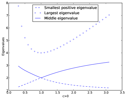
Figure 4: The three positive eigenvalues of the Laplacian of a 4-cycle with conductances $1$, $c$, $1/c$ and $(1+c^{2}-c)/(1+c^{2}+c)$.

It is reasonable to question whether the results presented are also true for the general cycle with $n$ vertices. More precisely one would expect that, for every $n$, if $T_{0}$ is the Laplacian for the $n$-cycle with constant conductances then

$$\lambda_{1}(T)\leq\lambda_{1}(T_{0})\leq\lambda_{n-1}(T_{0})\leq\lambda_{n-1}(T_{0}).$$ (16)

for every Laplacian $T$ on the cycle with $\rho(T)=\rho(T_{0})$. So far, we have not found a counterexample for that, and the numerical evidence also points in that direction. However, it does not seem plausible that the methods used for the case $n=3$ can be adapted in a simple way to establish the general case. Most likely, a different approach might be needed to obtain a general proof.

Hereby, we show graphical evidence in two particular situations for the $4$-cycle. It is straightforward to calculate the global resistance of the $n$ cycle with conductances $c_{i,j}$ to be equal to

$$\rho(T)=\frac{2(c_{0,1}c_{1,2}+c_{0,1}c_{2,3}+c_{0,1}c_{0,3}+c_{1,2}c_{2,3}+c_{1,2}c_{0,3}+c_{2,3}c_{0,3})}{c_{0,1}c_{1,2}c_{2,3}+c_{0,1}c_{1,2}c_{0,3}+c_{1,2}c_{2,3}c_{0,3}+c_{1,2}c_{2,3}c_{0,3}}$$

This gives $\rho(T_{0})=3$. The condition $\rho(T)=3$ determines each conductance as a function of the other three, in particular

$$c_{0,1}=\frac{3c_{1,2}c_{2,3}c_{0,3}-2(c_{1,2}c_{2,3}+c_{1,2}c_{0,3}+c_{2,3}c_{0,3})}{2(c_{1,2}+c_{2,3}+c_{0,3})-3(c_{1,2}c_{2,3}+c_{1,2}c_{0,3}+c_{2,3}c_{0,3}))}$$

For the particular example when shown in the next picture, the behaviour of the eigenvalues is shown in the plot of figure 4.

The second case considered is:

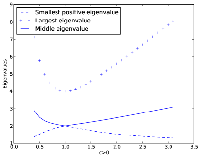
Figure 5: The three positive eigenvalues of the Laplacian of a 4-cycle with conductances $1$, $c$, $1/c$ and $(1+c^{2}-c)/(1+c^{2}+c)$.

The plot of the eigenvalues for this case is shown in figure 5.

As we see, these plots suggest that the eigenvalues have a similar behaviour to the one of the case $n=3$. Namely, that not only (16) might be true, but also that we could expect nice monotonic behaviours similar to the ones described in lemmas 1, 2 and 3.

References

• [1] T. Biyikoglu and J. Leylold. Faber–Krahn inequalities for trees. Journal of Combinatorial Theory. Series B., 97:159 –174.
• [2] T. Biyikoglu, J. Leylold, and P.F. Stadler. Laplacian Eigenvectors of Graphs. Springer.
• [3] I. Chavel. Isoperimetric Inequalities. Cambridge University Press.
• [4] P.G. Doyle and J.L. Snell. Random walks and electric networks. The Mathematical Association of America.
• [5] J. Friedman. Some geometric aspects of graphs and their eigenfunctions. Duke Mathematical Journal, 69:487 –525.
• [6] A. Henrot. Extremum Problems for Eigenvalues of Elliptic Operators. Birkhauser Verlag.
• [7] A. Katsuda and H. Urakawa. The Faber–Krahn type isoperimetric inequalities for a graph. Tohoku Math. J., (2) 51:267–281.
• [8] J. Kigami. Analysis on Fractals. Cambridge University Press.
• [9] J. Leydold. The geometry of regular trees with the Faber–Krahn property,. Discrete Math., 245:155 –172.
• [10] G. Pólya and Szego G. Isoperimetric Inequalities in Mathematical Physics. Princeton University Press.
• [11] R.S. Strichartz. Differential Equations on Fractals. Princeton University Press.