Nonlinear Schrödinger equations
and the universal description
of dispersive shock wave structure

Abstract.

The nonlinear Schrödinger (NLS) equation and the Whitham modulation equations both describe slowly varying, locally periodic nonlinear wavetrains, albeit in differing amplitude-frequency domains. In this paper, we take advantage of the overlapping asymptotic regime that applies to both the NLS and Whitham modulation descriptions in order to develop a universal analytical description of dispersive shock waves (DSWs) generated in Riemann problems for a broad class of integrable and non-integrable nonlinear dispersive equations. The proposed method extends DSW fitting theory that prescribes the motion of a DSW’s edges into the DSW’s interior, i.e., this work reveals the DSW structure. Our approach also provides a natural framework in which to analyze DSW stability. We consider several representative, physically relevant examples that illustrate the efficacy of the developed general theory. Comparisons with direct numerical simulations show that inclusion of higher order terms in the NLS equation enables a remarkably accurate description of the DSW structure in a broad region that extends from the harmonic, small amplitude edge.

1. Introduction

There has been a surge of interest recently in the subject of dispersive hydrodynamics and, in particular, dispersive shock waves (DSWs) (see [7, 19] and references therein). This has largely occurred thanks to the growing recognition of the fundamental nature and ubiquity of DSWs in physical applications: from shoaling tsunami waves [60, 3, 28] and internal undular bores in the ocean [56, 53, 29] and atmosphere [10, 49] to nonlinear diffraction patterns and optical shocks in laser beam propagation [62, 25, 11, 23, 66], quantum shocks in superfluids [13, 34, 51, 36], and nonlinear spin wave propagation in magnetic thin films [37]. On the other hand, the study of DSWs has revealed a number of challenging mathematical problems in the context of both integrable and non-integrable nonlinear wave equations.

A DSW is an expanding, modulated nonlinear wavetrain that connects two disparate hydrodynamic states (see Fig. 1). It can be viewed as a dispersive counterpart to the dissipative, classical shock. Hydrodynamic wave breaking singularities in dispersive media are generically resolved by DSWs. A DSW has a distinct multi-scale structure consisting of an oscillatory transition between two non-oscillatory—e.g., slowly varying or constant—states: one edge is associated with a solitary wave or soliton (for convenience, we use the term soliton regardless of the integrability of the governing equation) that is connected, via a slowly modulated periodic wavetrain, to a harmonic, small-amplitude wave at the opposite edge. The relative position (left/trailing or right/leading) of the soliton and harmonic edges determines the DSW orientation $d$, found in terms of the curvature of the linear dispersion relation as $d=-\hbox{sgn}[\partial_{kk}\omega_{0}(k,u_{0})]$ [15, 19]. Here, $\omega=\omega_{0}(k,u_{0})$ is the frequency of a small amplitude wave with wavenumber $k$ that propagates on the mean flow background $u_{0}$. The DSW shown in Fig. 1 has $d=1$ because the solitary wave is on the rightmost, leading edge. The shock structure of a DSW—an unsteady oscillatory wavetrain—is more complex than the stationary shock structure of a viscous shock wave. In particular, a DSW cannot be described by a traveling wave (ODE) solution of the nonlinear wave equation [15].

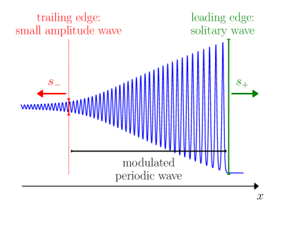
Figure 1. DSW expanding oscillatory structure in convex dispersive hydrodynamics with negative dispersion.

The rapidly oscillating structure of DSWs motivates the use of asymptotic, WKB-type, methods for its analytic description. One such method, known as Whitham modulation theory [63, 65] (see also [39]), is based on the averaging of dispersive hydrodynamic conservation laws over nonlinear periodic wavetrains leading to a system of first order quasilinear partial differential equations (PDEs). Whitham theory has proved particularly effective for the description of DSWs in both integrable and non-integrable systems. If the dispersive hydrodynamics are described by an integrable equation such as the Korteweg-de Vries (KdV) or nonlinear Schrödinger (NLS) equation, the associated Whitham system can be represented in a diagonal, Riemann invariant form [63, 24, 39]. This fact enabled Gurevich and Pitaevskii (GP) [32] to construct an explicit modulation solution for a DSW generated by a Riemann problem for the KdV equation. The GP construction is based on a self-similar, rarefaction wave solution of the KdV-Whitham equations. This modulation solution describes the interior shock structure of a DSW and reveals a monotonic change in the nonlinear wave’s wavenumber, mean, and amplitude as the DSW is spatially traversed.

For non-integrable dispersive equations, diagonalization of the associated modulation systems in terms of Riemann invariants is generally not possible, often presenting an insurmountable obstacle to the explicit determination of the Whitham system’s simple wave solution, although its existence requires only strict hyperbolicity and genuine nonlinearity. Consequently, the analytical description of a DSW’s interior structure has so far been limited to integrable systems or a detailed analysis of the Whitham modulation system in certain limiting regimes on a case-by-case basis [31, 18]. One can, however, explicitly determine key observables associated to each DSW edge, even for non-integrable equations. These observables include the DSW edge speeds and their associated wave parameters—the harmonic edge wavenumber and the soliton edge amplitude. The determination of these observables represents the fitting of a DSW to the long-time dynamics of piecewise constant, initial Riemann data. The DSW fitting method proposed in [16] (see also [19]) is based on a fundamental, generic property: the Whitham modulation equations admit exact reductions to a set of common, much simpler, analytically tractable equations in the limits of vanishing amplitude and vanishing wavenumber, which correspond to the harmonic and soliton DSW extremes (see Fig. 1). Therefore, the DSW fitting method can be viewed as a universal dispersive hydrodynamic analog to the Rankine-Hugoniot conditions for dissipative, viscous shocks. The key advantage of the method is that it involves neither the determination nor the analysis of the full Whitham system because the required zero-amplitude and zero-wavenumber reductions are available directly and are ultimately determined by the nonlinear, hyperbolic flux and the linear dispersion relation of the dispersive hydrodynamics. The method greatly expands the scope of DSW analysis as it is not reliant on integrability of the governing nonlinear dispersive equation via inverse scattering theory. It has been successfully applied to many non-integrable dispersive hydrodynamic systems. See, for example, [18, 17, 22, 12, 44, 33, 46, 35, 2]. Restrictions to the method’s applicability are related to possible violations of genuine nonlinearity (convexity) and strict hyperbolicity of the modulation system [44, 33].

Once the parameters of the leading and trailing edges have been determined by DSW fitting, wave modulation in the vicinity of these edges can be, in principle, determined by expanding the full Whitham system, for small amplitudes near the harmonic edge and small wavenumbers near the soliton edge [31, 18]. Such an asymptotic consideration, however, has a number of serious drawbacks due to the need to derive and analyze the full modulation system. Apart from being a potentially daunting technical task, this presents a major disadvantage to the whole procedure as it is system specific. It would therefore be highly desirable to have a more direct, widely applicable method for the determination of the DSW structure including modulation near the harmonic and soliton edges, which would complement and extend the existing general DSW fitting procedure.

In this paper, we develop a general method for the determination of the universal nonlinear DSW modulation—the DSW structure—near the harmonic edge. This asymptotic modulation provides crucial information about the variation of the amplitude in the DSW (i.e. the envelope of the oscillatory wavetrain) as well as other physical DSW parameters such as the wavenumber and mean flow. The modulation is universal because it is derived from the NLS equation, a universal model of weakly nonlinear, modulated dispersive wavetrains [5]. The present work takes advantage of the asymptotic overlap region in the vicinity of the DSW harmonic edge between the semiclassical, long-wave limit of the NLS equation and the small amplitude limit of the full Whitham modulation equations. The commonalities and differences between Whitham modulation theory and the NLS equation have been widely discussed in the literature (see, e.g., [47, 19]) but to the best of our knowledge, the overlap regime for the applicability of the two descriptions has never been used in practice, except very recently in [45]. While the Whitham equations describe modulations of fully nonlinear wavetrains, the NLS description is advantageous in the weakly nonlinear regime because it incorporates higher order dispersive effects of the wave envelope that are not accounted for in leading order Whitham theory.

We use the parameters obtained by DSW fitting applied to the harmonic edge as input information for a standard, small amplitude, multiple scales expansion that leads to the NLS equation for the wave’s envelope and phase. The specific information relevant to dispersive hydrodynamics consists of the NLS’ nonlinear and dispersion coefficients. The universal asymptotic modulation in a DSW is then found as a special vacuum rarefaction simple wave solution of the NLS equation in the long-wavelength, dispersionless limit, which is similar to the solution to the shallow water equations for the classical dam break problem with a dry downstream bed.

We consider several representative integrable and non-integrable examples to illustrate the efficacy of the developed general theory. Comparisons with direct numerical simulations show that the accuracy of the asymptotic description improves dramatically when higher order terms of the NLS equation are taken into account in the so-called HNLS equation. The HNLS equation was first derived in the nonlinear optics context [40, 41] but it is a universal equation that also arises in other applications including fluid dynamics [27, 54] and plasma physics [30]. We observe that in all considered examples, the vacuum rarefaction simple wave solution of the semi-classical, dispersionless HNLS equation provides a remarkably accurate description of the DSW modulation, and therefore the DSW structure, in a broad vicinity of the harmonic edge. Finally, we show that convexity of the linear dispersion relation for the original dispersive hydrodynamics plays a key role in the determination of DSW stability via the focusing/defocusing character of the associated NLS equation.

The paper is organized as follows. We begin in Sec. 2 with a brief outline of the necessary elements of DSW modulation theory and, in particular, the DSW fitting method for the determination of the DSW harmonic edge in scalar dispersive hydrodynamic systems. Section 3 develops an asymptotic, multiple scales expansion in the vicinity of the DSW harmonic edge that leads to the NLS equation. This is used to derive the universal, first order approximation of the DSW modulation as a vacuum rarefaction simple wave solution of the long-wave, dispersionless limit of the NLS equation. We then extend the first order analysis by including higher order terms in the multiple scales expansions in Sec. 4. This results in the HNLS equation for which we find the appropriate simple wave solution in the long-wavelength limit. Section 5 is devoted to applications to several representative examples. The examples include the KdV equation, the conduit equation that models the interfacial dynamics of a rising, buoyant, viscous fluid within another miscible, high viscosity contrast fluid [52, 44], and the Serre equations for fully nonlinear shallow water waves [55, 58, 18]. The latter two equations are non-integrable. We complete the paper with a summary, and discussion of further directions in Sec. 6. Appendices A and B detail the multiple scales derivations of the NLS and HNLS equations for the conduit equation and the Serre system. Appendix C is devoted to a brief description of numerical methods used for simulations.

2. Dispersive shock waves: modulation theory

In this Section, we outline the elements of DSW modulation theory that are necessary for developments in subsequent sections. A detailed exposition can be found in [19, 15].

2.1. Modulation equations and the matching regularization of the Riemann problem

We consider scalar dispersive hydrodynamics generically described by the equation

(1) $$u_{t}+f(u)_{x}+D[u]_{x}=0$$

with $f^{\prime\prime}(u)\neq 0$. The dispersive operator $D$ (generally integro-differential) is assumed to have the property that equation (1) admits the real-valued linear dispersion relation $\omega=\omega_{0}(k,u_{0})$ with long-wave expansion

(2) $$\omega_{0}(k,u_{0})=f^{\prime}(u_{0})k+\zeta k^{3}+o(k^{3}),\quad k\ll 1,\quad\zeta\neq 0$$

for small-amplitude waves proportional to $e^{i(kx-\omega t)}$ and propagating on a constant (or slowly varying) background $u=u_{0}$. We shall initially assume that the dispersion relation is purely convex or concave, so that $\partial_{kk}\omega_{0}\neq 0$. Suppose equation (1) has a three-parameter periodic traveling wave solution and at least two local conservation laws. These basic requirements are quite generic and are satisfied by many dispersive hydrodynamic equations arising in applications. When the dispersive hydrodynamics admit the above properties, we say that they are of KdV type.

We shall consider the evolution of Riemann step initial data

(3) $$u(x,0)=\left\{\begin{array}[]{ll}u_{-},&x<0\\[6.0pt] u_{+},&x>0\end{array}\right.$$

for Eq. (1). Our consideration will be based upon the fundamental assumption that the initial step (3) is regularized in the long-time limit by the emergence of three distinct regions in the $x$-$t$ upper half space-time plane so that the solution is given by two constant states $u=u_{-}$ and $u=u_{+}$ that are separated by an expanding DSW region (see Fig. 2). Within this region, the solution has an oscillatory structure described by a modulated, locally periodic wavetrain that exhibits a solitary wave at one edge and a vanishing amplitude linear wave at the opposite edge (recall Fig. 1). This asymptotic structure of the Riemann problem solution has been rigorously recovered for a number of integrable equations (see, e.g., [14, 38]). For non-integrable equations such as the Serre system [18] or conduit equation [44], the existence of a modulated, periodic, single phase wave structure of a DSW is a plausible assumption which can be inferred from numerical simulations.

We assume that Eq. (1) admits a three parameter family of periodic, traveling wave solutions $u(x,t)=U(\theta)$, where $\theta=kx-\omega t$, $k$ being the wavenumber and $\omega$ the wave frequency, so that $U(\theta+2\pi)=U(\theta)$. It is convenient to use the period mean ${\overline{u}}=(2\pi)^{-1}\oint U{\rm d}\theta$, the amplitude $a=u_{\rm max}-u_{\rm min}$ and the wavenumber $k$ as a basic parameter set, i.e., $U(\theta)\equiv U(\theta;{\overline{u}},a,k)$; all other physical parameters, such as the frequency $\omega$ or the mean square $\overline{u^{2}}$ are functions of the basic triple $({\overline{u}},a,k)$. We also assume that the solution $U(\theta;{\overline{u}},a,k)$ has two asymptotic limits: (i) when $a\to 0$ it transforms into a linear wave on the background $u=u_{0}$ with the dispersion relation $\omega=\omega_{0}(k,u_{0})$; (ii) when $k\to 0$ it transforms into an exponentially decaying solitary wave. Examples of dispersive equations whose periodic solutions satisfy the above properties include KdV, modified KdV, the conduit equation and others.

We now consider a solution of Eq. (1) represented by the $2\pi$-periodic traveling wave with slow $(x,t)$-dependence of $({\overline{u}},a,k)$. This slowly varying traveling wave is characterised by the generalized phase $\theta(x,t)$ so that the local wavenumber and frequency are given by $k=\theta_{x}$ and $\omega=-\theta_{t}$ respectively. The variations of $({\overline{u}},a,k)$ satisfy the Whitham modulation equations [65], which can be obtained by applying multiple scales expansions or, equivalently, by averaging two independent conservation laws of (1) over the periodic family and completing the system with the consistency equation $\theta_{xt}=\theta_{tx}$ that yields wave number conservation $k_{t}+\omega_{x}=0$. The same set of modulation equations can be derived via an averaged variational principle [64]. Assuming non-vanishing Jacobians, the Whitham system can be represented as a system of quasilinear first order equations

(4) $$\left(\begin{array}[]{c}{\overline{u}}\\ a\\ k\\ \end{array}\right)_{t}+\mathrm{A}({\overline{u}},a,k)\left(\begin{array}[]{c}{\overline{u}}\\ a\\ k\\ \end{array}\right)_{x}=\left(\begin{array}[]{c}0\\ 0\\ 0\\ \end{array}\right),$$

where $\mathrm{A}({\overline{u}},a,k)\in\mathbb{R}^{3\times 3}$ is a matrix. We initially assume hyperbolicity so that the eigenvalues $V_{1}\leq V_{2}\leq V_{3}$ of $\mathrm{A}$ are real and the eigenvectors $\{{\bf r}_{j}~{}|~{}\mathrm{A}{\bf r}_{j}=V_{j}{\bf r_{j}},~{}j=1,2,3\}$ form a basis in $\mathbb{R}^{3}$.

In the context of a DSW that is described by a modulated periodic wave solution, the Whitham equations (4) are subject to free boundary (matching) conditions [32, 16]

(5) $$\begin{split}x=x_{-}(t):\qquad a=0,\ \ {\overline{u}}=u_{-}\,,\\ x=x_{+}(t):\qquad k=0,\ \ {\overline{u}}=u_{+}\,,\end{split}$$

thus ensuring continuity of the mean flow ${\overline{u}}$ at the unknown DSW edges $x=x_{\pm}(t)$. Outside the DSW region $x_{-}(t)\leq x\leq x_{+}(t)$, the solution is given by $u=u_{-}$ for $x<x_{-}(t)$ and $u=u_{+}$ for $x>x_{+}(t)$. Here, for specificity, we have assumed a positive DSW orientation (see Fig.  1) so that the harmonic edge is trailing, $x=x_{-}(t)$, and the soliton edge is leading, $x=x_{+}(t)$. We also assume concave flux, $f^{\prime\prime}(u)>0$, which implies the admissibility or causality condition $u_{-}>u_{+}$ for a compressive DSW [15, 19]. The cases of positive dispersion that yield either a negative DSW orientation, $d=-1$, or convex flux $f^{\prime\prime}(u)<0$ (which implies $u_{-}<u_{+}$ for compressive DSW formation) can be considered in a similar fashion.

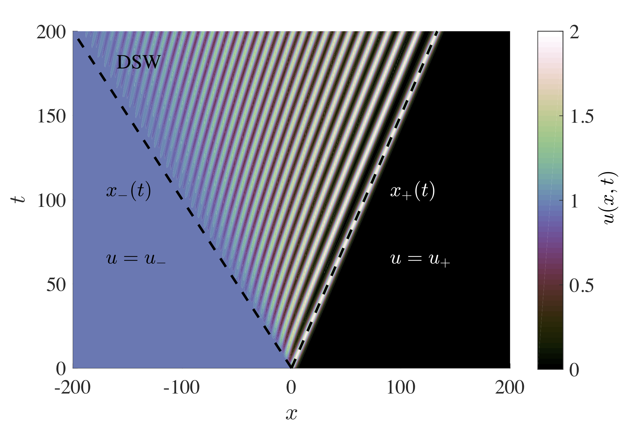
Figure 2. Contour plot of the asymptotic KdV DSW solution obtained by GP [32] for $u_{-}=1$, $u_{+}=0$.

The hydrodynamic scaling invariance $x\to ax$, $t\to at$ of both the modulation equations (4) and initial conditions (3), together with hyperbolicity, necessitate a self-similar, simple wave modulation solution. To satisfy the matching conditions (5), the modulation solution must be a 2-wave rarefaction curve [16, 19] given by

(6) $$V_{2}({\overline{u}},a,k)=x/t,\qquad I_{1}({\overline{u}},a,k)=0,\quad I_{2}({\overline{u}},a,k)=0,$$

where $I_{1,2}$ are integrals of the Whitham system (4) on the solution curve. The integrals are parametrized by the Riemann data $u_{\pm}$, i.e., $I_{1}(u_{-},0,k_{-})=0$ and $I_{2}(u_{+},a_{+},0)=0$ determine the trailing edge harmonic wavenumber $k_{-}$ and the leading edge soliton amplitude $a_{+}$. For the KdV equation solution, Eq. (6) was found explicitly by GP [32] in terms of Riemann invariants that are available for the KdV-Whitham system owing to its complete integrability [24], unbeknownst to Whitham who was able to determine the Riemann invariants explicitly via an involved, direct calculation [63] (see also [6, 39]). The DSW edge speeds $s_{\pm}$ are constant and follow from the modulation solution (6) in the $a\to 0$ (harmonic, trailing edge) and $k\to 0$ (soliton, leading edge) limits by evaluating the linear group velocity and soliton phase velocity, respectively. The $(x,t)$-contour plot of the GP solution to the Riemann problem for the KdV equation $u_{t}+uu_{x}+u_{xxx}=0$ illustrates the described modulation theory setting in Fig. 2.

The above outlined construction of the DSW modulation solution for scalar equations (1) can be extended to systems describing bidirectional dispersive hydrodynamics, e.g., the Serre shallow water equations, the generalized NLS equation and other systems. See, e.g., [16, 20, 18, 33].

2.2. The determination of the harmonic edge: DSW fitting

Modulation systems (4) obtained by averaging dispersive hydrodynamic systems (1) exhibit an important general property: they admit exact reductions to lower order quasilinear systems in the harmonic ($a\to 0$) and soliton ($k\to 0$) limits (recall that these two limits correspond to special wave regimes realized at the DSW edges [31, 16, 19]). Importantly, these exact reductions are often available directly, without the necessity to derive the full modulation system. Another fundamental fact is that in the Riemann problem, the DSW edges are characteristics when the modulation system (4) is hyperbolic. As a result, the speeds $s_{\pm}$ of the harmonic and soliton edges can be obtained from the analysis of the reduced modulation systems. The corresponding technique proposed in [16] is sometimes referred to as the DSW fitting method.

Determining the harmonic edge via the DSW fitting method is particularly simple. Indeed, the harmonic reduction ($a=0$) of the modulation system (4) can be shown to be universally represented in the physically transparent form

(7) $${\overline{u}}_{t}+f({\overline{u}})_{x}=0,\qquad k_{t}+[\omega_{0}(k,{\overline{u}})]_{x}=0.$$

Then the DSW harmonic edge speed coincides with the linear group velocity for the edge parameters ${\overline{u}}=u_{-}$, $k=k_{-}$:

(8) $$s_{-}=\partial_{k}\omega_{0}(k_{-},u_{-})\quad\hbox{where}\quad k_{-}=K(u_{-}),$$

$K({\overline{u}})$ being the harmonic edge wavenumber locus function, which is determined as follows. Let the value ${\overline{u}}=u_{+}$ at the DSW soliton edge be fixed. Then the function $K({\overline{u}})$ is found from the ODE

(9) $$\frac{dK}{d{\overline{u}}}=\left[\frac{\partial_{{\overline{u}}}\omega_{0}}{f^{\prime}({{\overline{u}}})-\partial_{k}\omega_{0}}\right]_{k=K},\quad K(u_{+})=0.$$

The ODE (9) follows by integrating the differential associated with the group velocity characteristic of Eq. (7) on the DSW harmonic edge. It specifies a relation between admissible values of $k$ and ${\overline{u}}$ along this edge. The initial condition in (9) follows from the GP matching conditions (5) (see [16, 19] for details).

The determination of the soliton edge is analogous, although it involves some nontrivial change of variables which we do not describe here (see [16, 19]). The extension of scalar DSW fitting to bidirectional, Eulerian dispersive hydrodynamic systems has been developed in [16, 33]. The DSW fitting procedure is subject to certain admissibility conditions derived from the monotonicity requirement for the relevant real characteristic velocity along the integral curve (6), i.e., the modulation system must be genuinely nonlinear and strictly hyperbolic along the entire integral curve [44, 33]. Therefore, the DSW fitting construction is not reliant upon the integrability of the dispersive hydrodynamic evolution equation (1), it only requires strict hyperbolicity and genuine nonlinearity of the modulation system (4).

3. Small amplitude DSW regime and the NLS equation

We shall be interested in the region of a DSW adjacent to the harmonic edge $x=s_{-}t$, where the oscillation amplitude $a$ is relatively small. One can, in principle, expand the Whitham equations (4) in powers of $a$ for $a\ll 1$ and solve them by seeking a solution in powers of the amplitude, subject to the matching condition (5) at $x=s_{-}t$. This programme has been to some extent realized in [31, 18] for several non-integrable dispersive hydrodynamic systems, including the equations for ion-acoustic and magneto-acoustic waves in collisionless plasma and the Serre equations for fully nonlinear dispersive shallow water waves. In all cases, the full modulation system (4) (or its bi-directional generalization) was derived, and then reduced to an abstract, model Whitham system for $a$ and $k$ (see [65], Ch. 16.15) involving an effective nonlinear frequency correction $\omega_{2}(k,u_{-})a^{2}$ to the linear dispersion relation $\omega_{0}(k,u_{-})$. As a result, the first order DSW modulation near the harmonic edge was determined, including the linear growth of the amplitude with distance. This approach, however, has a major drawback, due to its reliance on the full modulation system in each case while only the small amplitude expansion is actually used.

Here, instead of deriving the full modulation system and making subsequent small amplitude expansions, we perform an appropriate small amplitude expansion directly on the original system and then derive modulation equations for weakly nonlinear periodic (Stokes) waves [65]. Slow modulations of almost monochromatic Stokes waves for a broad class of nonlinear dispersive systems are known to be described by the nonlinear Schrödinger equation or its higher order versions [5, 1, 67]). Consequently both Whitham modulation theory and an NLS description can be used in the inner vicinity of the DSW harmonic edge. Moreover, since a DSW is described by a rarefaction wave solution of the Whitham equations, the counterpart NLS description will reduce to finding a simple wave solution to the dispersionless limit of the corresponding NLS equation or one of its higher order versions.

It is instructive to start with an outline of the standard derivation of the NLS equation. See, e.g., [1] for examples and further details. Let $\varepsilon$ be a small parameter characterizing the wave amplitude. We seek the solution of the dispersive hydrodynamic equation (1) in the form of an asymptotic expansion about the constant $u_{0}$ for a nearly monochromatic wave with the dominant carrier wavenumber $k$

(10) $$u=u_{0}+\varepsilon u_{1}+\varepsilon^{2}u_{2}+\varepsilon^{3}u_{3}+\dots,$$

where

$$u_{1}=A(X,T_{1},T_{2})e^{i(kx-\omega t)}+\hbox{c.c.},\ X=\varepsilon x,T_{1}=\varepsilon t,T_{2}=\varepsilon^{2}t.$$

Substituting expansion (10) into Eq. (1) and collecting terms in powers of $\varepsilon$, we obtain the linear dispersion relation $\omega=\omega_{0}(k,u_{0})$ at the first order. To eliminate secular terms at $O(\varepsilon^{2})$, we require that the complex wave envelope move with the group velocity

(11) $$A_{T_{1}}+\partial_{k}\omega_{0}A_{X}=0.$$

The NLS equation arises as the condition for removal of secular terms at $O(\varepsilon^{3})$ and has the form

(12) $$iA_{T_{2}}+\beta A_{XX}+\gamma|A|^{2}A=0,$$

where $\beta(k,u_{0})=\tfrac{1}{2}\partial_{kk}\omega_{0}$. We also obtain the variation of the mean ${\overline{u}}-u_{0}\sim\varepsilon^{2}b_{1}(k,u_{0})|A|^{2}$ as a by-product of the $O(\varepsilon^{3})$ calculation. Here, the factors $b_{1}$ and $\gamma$ has no general expressions.

Although the outlined above derivation is standard, it can be quite laborious, especially for systems. The difficult part of the derivation is the determination of the nonlinear coefficient $\gamma(k,u_{0})$, but this computation can be readily performed with the aid of a symbolic algebra package such as Mathematica. See Appendix B for an outline of the calculations for the Serre system. In fact, $\gamma$ is precisely the sought for nonlinear frequency correction $\omega_{2}(k,\overline{u})$ mentioned earlier that is obtained in a weakly nonlinear analysis of the Whitham equations. Equations for $A_{T_{1}}$ and $A_{T_{2}}$ can be combined into a single equation for the un-scaled envelope $\tilde{A}(x,t)$ defined by

(13) $$\tilde{A}(x,t)=\varepsilon A(\epsilon x,\epsilon t,\epsilon^{2}t).$$

Hence, one has the following substitution rules:

(14) $$\tilde{A}_{x}=\varepsilon^{2}A_{X},\;\tilde{A}_{t}=\varepsilon^{2}A_{T_{1}}+\varepsilon^{3}A_{T_{2}},\;|\tilde{A}|^{2}=\varepsilon^{2}|A|^{2}\,.$$

The envelope of the wave packet $u=u_{0}+\tilde{A}(x,t)e^{i(kx-\omega_{0}t)}+\rm{c.c.}$ is then governed by the equation:

(15) $$i\tilde{A}_{t}+i\partial_{k}\omega_{0}\tilde{A}_{x}+\beta\tilde{A}_{xx}+\gamma|\tilde{A}|^{2}\tilde{A}=0\,.$$

The sign of the product $\beta\gamma$ determines the NLS type: if $\beta\gamma>0$ the equation is attractive or focusing and describes the envelope of a modulationally unstable wave while for $\beta\gamma<0$ it is repulsive or defocusing and describes the envelope of a modulationally stable wave.

To apply the NLS equation to the description of the DSW harmonic edge vicinity, we assume in (10):

$$u_{0}=u_{-},\quad k=k_{-},\quad\varepsilon u_{1}=\tilde{A}(\chi,t)\exp[i(k_{-}x-\omega_{0}(k_{-},u_{-})t)]+\hbox{c.c.},$$

where $\chi=x-\partial_{k}\omega_{0}(k_{-},u_{-})\,t=x-s_{-}t$. The DSW-NLS equation for $\tilde{A}$ is then

(16) $$i\tilde{A}_{t}+\beta(k_{-},u_{-})\tilde{A}_{\chi\chi}+\gamma(k_{-},u_{-})|\tilde{A}|^{2}\tilde{A}=0,$$

where the dependence of $k_{-}$ on the Riemann data $u_{\pm}$ is obtained by DSW fitting.

We introduce the Madelung transformation $\tilde{A}=\sqrt{\rho}e^{i\phi}$, $v=\phi_{\chi}$ to cast the NLS equation (16) in dispersive-hydrodynamic form

(17) $$\begin{split}&\rho_{t}+2\beta(\rho v)_{\chi}=0,\\ &v_{t}+2\beta vv_{\chi}-\gamma\rho_{\chi}-\beta(\sqrt{\rho}_{\chi\chi}/\sqrt{\rho})_{\chi}=0,\end{split}$$

where $v\sim k-k_{-}$, and $\sqrt{\rho}=|\tilde{A}|\sim a/4$ in the DSW context (we recall that $a=u_{\rm max}-u_{\rm min}$). The DSW modulation solution is a rarefaction curve of the Whitham equation so the relevant NLS solution must also be a rarefaction wave described by the long-wave, dispersionless limit. Neglecting the dispersive term in (17) we obtain

(18) $$\begin{split}&\rho_{t}+2\beta(\rho v)_{\chi}=0,\\ &v_{t}+2\beta vv_{\chi}-\gamma\rho_{\chi}=0.\end{split}$$

The characteristic velocities are $\beta v\pm\sqrt{-2\beta\gamma\rho}$, so the system is hyperbolic if $\beta\gamma<0$ and elliptic if $\beta\gamma>0$, consistent with the defocusing and focusing character of the NLS equation (12), respectively. We assume for now that $\beta\gamma<0$, so that the system (18) is equivalent to the shallow water equations.

We now need to specify boundary conditions for the dispersionless NLS equation (18) at the DSW harmonic edge. This is done using the GP matching conditions (5) and the DSW fitting data. In the original modulation variables, we have from (5)

(19) $$x=s_{-}t:\qquad a=0,\qquad k=k_{-}.$$

Note that, unlike the free boundary in (5), the boundary in (19) is known from DSW fitting. Translating (19) into the variables of (18), we arrive at a boundary value problem for the vacuum rarefaction wave

(20) $$\chi=0,~{}t>0:\quad\rho=0,\quad v=0.$$

We are now looking for a self-similar rarefaction wave solution of the shallow water equations (18) subject to the boundary conditions (20). There are two such non-trivial solutions—the fast and slow waves. The correct one is chosen by the admissibility condition that the wavenumber decrease monotonically as the DSW is traversed from the harmonic to the soliton edge, i.e., $dk/da<0$ or, equivalently, $dv/d\rho<0$. Then the required solution of (18) is given by

(21) $$\sqrt{\rho}=\frac{1}{3\sqrt{-2\beta\gamma}}\left|\frac{\chi}{t}\right|;\quad v=\frac{1}{3\beta}\frac{\chi}{t}\,.$$

Using the dispersionless NLS solution (21) and the expansions (10), we recover the leading order behaviors of the amplitude $a$ and the wavenumber $k$ near the DSW harmonic edge in terms of the dispersion and nonlinearity coefficients $\beta$ and $\gamma$ of the associated NLS equation (16)

(22) $$a\sim\frac{4}{3}\frac{1}{\sqrt{-2\beta\gamma}}|x/t-s_{-}|,\quad k-k_{-}\sim\frac{1}{3\beta}\left(x/t-s_{-}\right).$$

We also recover the variation of the mean:

(23) $$\overline{u}-u_{-}\sim b_{1}(k_{-},u_{-})\,\rho\propto\left(x/t-s_{-}\right)^{2}.$$

Equation (22) is the universal description of the DSW envelope (with “martini-glass” shape [42, 19]) near the harmonic edge for systems with convex dispersion ($\beta\neq 0$).

Solution (22) is valid when $\beta\gamma<0$, which is the hyperbolicity condition for the dispersionless NLS system (18) and can be interpreted as a necessary condition for DSW modulational stability. For non-convex dispersion relations, the sign of $\beta$ can change and the system may exhibit an unstable behavior described by the focusing NLS equation where $\beta\gamma>0$. An example of such behavior has been recently reported in [45], where it was shown that nonconvexity of the linear dispersion relation for the conduit equation implies an elliptic regime for the associated Whitham equations in a certain region of parameter phase space. This gives rise to modulationally unstable dynamics that can be described by the focusing NLS equation in the small amplitude regime.

For systems with non-convex dispersion, the study of DSW behavior near the zero dispersion point $\beta=0$ necessitates inclusion of higher order terms in the associated NLS equation. It turns out that the inclusion of such terms is beneficial even outside the non-convex, zero-dispersion regime, as we now demonstrate.

4. Higher order NLS approximation

We can include higher order nonlinear/dispersive effects in the asymptotic expansion (10) by introducing a third, slower time scale $T_{3}=\varepsilon^{3}t$ and assuming $u_{1}=A(X,T_{1},T_{2},T_{3})e^{i(kx-\omega t)}+{\rm c.c.}$ The cancellation of secular terms at $O(\varepsilon^{4})$ then gives

$$A_{T_{3}}+\delta A_{XXX}+\lambda|\tilde{A}|^{2}A_{X}+\mu A^{2}A^{*}_{X}=0\,,$$

where $\delta(k,u_{0})=-\partial_{kkk}\omega_{0}/6$ and $A^{*}$ is the complex conjugate of $A$. Once again, the laborious part of the computation consists in finding the coefficients $\lambda(k,u_{0})$ and $\mu(k,u_{0})$. Written in the moving reference frame $(\chi,t)$ (cf. Appendix A for the derivation of the un-scaled equation), where $\chi=x-\partial_{k}\omega_{0}(k,u_{0})t$ (recall Eq. (16)), the resulting equation is the higher order NLS, or HNLS, equation

(24) $$i\tilde{A}_{t}+\beta\tilde{A}_{\chi\chi}+\gamma|\tilde{A}|^{2}\tilde{A}+i\delta\tilde{A}_{\chi\chi\chi}+i\lambda|\tilde{A}|^{2}\tilde{A}_{\chi}+i\mu\tilde{A}^{2}\tilde{A}^{*}_{\chi}=0,$$

initially derived as an improvement to the standard NLS equation for signal propagation in optical fibers [41]; it also arises in geophysical fluid dynamics [27] and other areas. See [54] and references therein. In the context of the description of a DSW, we set $u_{0}=u_{-}$ and $k=k_{-}(u_{-},u_{+})$ from DSW fitting in the coefficients $\beta$, $\gamma$, $\delta$, $\lambda$, $\mu$.

Similar to the previous section, we cast the HNLS equation (24) in dispersive hydrodynamic form using the Madelung transform $\tilde{A}=\sqrt{\rho}e^{i\int v\,d\chi}$. Upon neglecting dispersive terms, we obtain the following quasilinear system for long waves

(25) $$\begin{split}&\rho_{t}+\left(2\beta\rho v-3\delta\rho v^{2}+(\lambda+\mu)\rho^{2}/2\right)_{\chi}=0,\\ &v_{t}+\left(\beta v^{2}-\delta v^{3}-\gamma\rho+(\lambda-\mu)\rho v\right)_{\chi}=0.\end{split}$$

As expected, the system (25) is equivalent to the shallow water equations (18) when $\delta=\lambda=\mu=0$. In the context of DSWs, the dispersionless limit (25) of the HNLS equation should be considered with the same vacuum rarefaction conditions (20) augmented by the DSW admissibility inequality $dv/d\rho<0$.

Before we proceed with the integration of system (25), let us briefly discuss its structure. The characteristic velocities are

(26) $$\begin{split}V_{\pm}(\rho,v)&=\lambda\rho+2\beta v-3\delta v^{2}\pm\rho\sqrt{D(\rho,v)},\\ D(\rho,v)&=\mu^{2}-2(\beta-3\delta v)(\gamma-(\lambda-\mu)v)/\rho\end{split}.$$

and the associated right eigenvectors are

(27) $$\mathbf{R}_{\pm}=\left(-\mu\rho\pm\rho\sqrt{D(\rho,v)},\gamma-(\lambda-\mu)v\right)^{T},$$

implying that the system (25) is hyperbolic in the region $(\rho,v)$ where $\rho>0$, the discriminant is positive $D>0$, and $\gamma\neq(\lambda-\mu)v$ so that $\mathbf{R}_{\pm}$ are independent. In the small amplitude regime ($\rho,|v|\ll 1$), we recover the standard hyperbolicity condition $\beta\gamma<0$ since $\beta,\gamma\neq 0$. Consequently, the DSW modulation near the harmonic edge is determined by the similarity solution of (25),

(28) $$V_{d}(\rho,v(\rho))=\frac{\chi}{t},$$

where $d=-\hbox{sgn}\ \beta$ is the DSW orientation and the dependence $v(\rho)$ is determined by the characteristic ODE

(29) $$\frac{dv}{d\rho}+\frac{\mu-d\sqrt{D(\rho,v)}}{2(\beta-3\delta v)}=0,\quad v(0)=0.$$

As a by-product of the multi-scale expansion to order $O(\varepsilon^{4})$, we obtain a higher order correction to the mean value (recall (23)) described by the new expression

(30) $${\overline{u}}-u_{-}\sim\rho(b_{1}+b_{2}v),$$

where $b_{1}$ has been obtained at the previous order ($O(\varepsilon^{3})$), and $b_{2}$ is determined as a by-product of the $O(\varepsilon^{4})$ computation.

We now obtain the second-order expansion of the simple wave modulation solution (28), (29) near $\chi=0$ for small $\rho$, $v$, which will improve the first-order NLS result (22) in the vicinity of the harmonic edge. Seeking the solution of (28), (29) in the form of a series in powers of $\chi/t$, we obtain universal asymptotic expressions for the DSW amplitude and wavenumber modulations (cf. (22))

(31) $$\begin{split}&a=\frac{4}{3\sqrt{-2\beta\gamma}}\left|\frac{\chi}{t}\right|+\hbox{sgn}\ \beta\ \frac{4(2\gamma\delta/\beta+\lambda-\mu)}{9(-2\beta\gamma)^{3/2}}\left(\frac{\chi}{t}\right)^{2}+O\left[\left(\frac{\chi}{t}\right)^{3}\right],\\ &k=k_{-}+\frac{1}{3\beta}\frac{\chi}{t}+\frac{7\delta+\beta\lambda/\gamma}{36\beta^{3}}\left(\frac{\chi}{t}\right)^{2}+O\left[\left(\frac{\chi}{t}\right)^{3}\right].\end{split}$$

We note that it is implicit in the expansions (31) that $|\beta(k_{-},u_{-})|=O(1)$, which is the case for dispersive hydrodynamic equations with a convex dispersion relation. For systems with non-convex dispersion such as the Benjamin-Bona-Mahony equation [4] or the conduit equation [52, 44], the behaviour near the zero-dispersion point, $\beta(k_{-},u_{-})=0$ captured by HNLS equation (24) requires a separate consideration, which is beyond the scope of the present paper.

For convex dispersive hydrodynamics, the second order approximation (31) formally delivers the same accuracy in the description of the vicinity of the DSW harmonic edge as the HNLS equation (24) itself. However, comparisons with results of direct numerical simulations of the Riemann problem for the example dispersive hydrodynamic equations in the next Section show that the simple wave solution (28), (29) of the full dispersionless HNLS (25) exhibits better agreement with numerical solution than the expansion (31). Remarkably, this agreement holds over a significant portion of a DSW, where the amplitude is not small and the HNLS description, let alone the expansions (31), are formally not expected to be applicable.

5. NLS description of dispersive shock waves: Examples

We now demonstrate the effectiveness of the developed general approach by applying it to several specific dispersive hydrodynamic systems and comparing the results with direct numerical simulations of the corresponding Riemann problems.

5.1. Korteweg-de Vries equation

As a first example, we consider the KdV equation

(32) $$u_{t}+uu_{x}+u_{xxx}=0$$

with Riemann initial data (3). The aim here is to compare the results of the developed asymptotic approach with the known GP modulation solution [32].

The KdV linear dispersion relation is

(33) $$\omega_{0}(k,u_{0})=u_{0}k-k^{3}.$$

The multiple scales asymptotic expansion of (32) leading to the NLS equation for KdV weakly nonlinear wavepackets is standard and can be found in the literature, see e.g. [1, 8]. The coefficients in (12) and (23) are

(34) $$\beta=-3k,\quad\gamma=\frac{1}{6k},\quad b_{1}=-\frac{1}{3k^{2}}.$$

We also derive the coefficients of the HNLS equation (24) and the associated higher order correction of the mean value (30) [8]

(35) $$\delta=1,\quad\lambda=-\frac{1}{3k^{2}},\quad\mu=-\frac{1}{2k^{2}},\quad b_{2}=\frac{2}{3k^{3}}.$$

The trailing edge wavenumber is readily obtained from DSW fitting (see [16] and Sec. 2.2). Solving the ODE (9), we obtain $k_{-}=K(u_{-})$ in the form

(36) $$k_{-}=\sqrt{\frac{2}{3}\Delta}\quad\text{with}\quad\Delta=u_{-}-u_{+}\,,$$

which yields the harmonic edge velocity

(37) $$s_{-}=\partial_{k}\omega_{0}(k_{-},u_{-})=u_{-}-2\Delta\,.$$

Substituting (35), (36) into (30) , (31), we obtain the second order expansions

(38) $$a = \frac{4}{3}\frac{\chi}{t}-\frac{1}{27\Delta}\left(\frac{\chi}{t}\right)^{2}+O\left[\left(\frac{\chi}{t}\right)^{3}\right],$$

(39) $$k = \sqrt{\frac{2\Delta}{3}}-\frac{1}{3\sqrt{6\Delta}}\frac{\chi}{t}-\frac{13}{216\sqrt{6}\Delta^{3/2}}\left(\frac{\chi}{t}\right)^{2}+O\left[\left(\frac{\chi}{t}\right)^{3}\right],$$

(40) $${\overline{u}} = u_{-}-\frac{1}{18\Delta}\left(\frac{\chi}{t}\right)^{2}-\frac{5}{324\Delta^{2}}\left(\frac{\chi}{t}\right)^{3}+O\left[\left(\frac{\chi}{t}\right)^{4}\right],$$

which agree with the corresponding expansions of the exact GP solution [32].

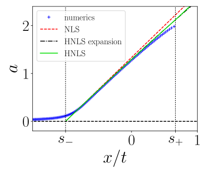
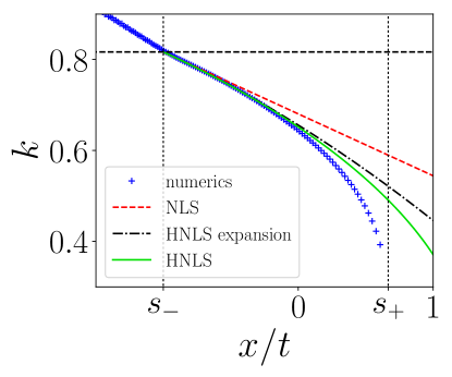
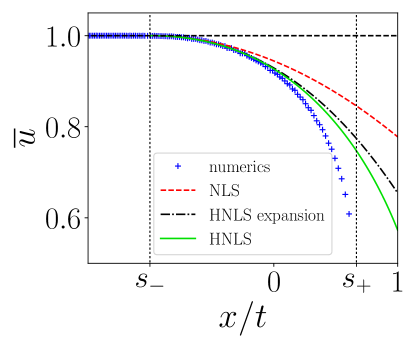
Figure 3. Amplitude, wavenumber, and mean field profiles for the KdV Riemann problem with $u_{-}=1$ and $u_{+}=0$. Comparison between direct numerical simulations at $t=500$ (blue pluses), the NLS/HNLS asymptotic descriptions given by (i) expansions (38)–(40) with the first order (NLS) approximation (dashed red line) and the second order (HNLS) approximation (dash-dotted black line) and (ii) the exact simple wave solution Eqs. (28), (29) of the dispersionless HNLS equation (solid green line). The horizontal black dashed lines correspond to the values of the corresponding fields in the harmonic limit: $a=0$, $k=k_{-}$ and ${\overline{u}}=u_{-}$.

The comparison between the exact simple wave solution (28), (29) of the dispersionless HNLS equation (25) with coefficients (34), the asymptotic expansion (38)–(40), and the direct numerical solution of the KdV Riemann problem is displayed in Fig. 3.

The numerical method used in the simulations is detailed in Appendix D. Although the NLS description is formally limited to the small-amplitude regime in the vicinity of the DSW harmonic edge, the KdV DSW amplitude is almost linear for $x/t\in[s_{-},s_{+}]$, so the term linear in $x/t$ in (38) fits almost the entire DSW with good accuracy. It is no longer the case for the wavenumber and the mean flow: good agreement between numerics and the first order (NLS) approximation is observed only in the vicinity of the trailing edge, but the second order expansions (39), (40) exhibit better agreement with the direct KdV numerics over a broader $x/t$ interval. The agreement further improves when the full solution (28), (29) of the dispersionless HNLS equation is used where all modulation parameters fit almost the entire DSW with good accuracy, with the exception of some vicinity of the leading edge, where $k\to 0$ and ${\overline{u}}\to u_{+}$ logarithmically in $\chi/t$ [32], behavior that cannot be captured by the expansions (39), (40).

We should make an important comment regarding the comparison of the behavior of the DSW oscillations near the harmonic edge with the results of modulation theory. We can see from Fig. 3, left panel, that there is some deviation of the envelope profile in a close vicinity of the trailing edge from linear behavior $a\propto(x/t-s_{-})$ that is predicted by modulation theory. In particular, the amplitude of the oscillations is not exactly zero for $x/t\leq s_{-}$. This discrepancy between the DSW modulation solution and the exact oscillation behavior is known, having been studied for the KdV equation in detail in [26] where it was shown that the envelope amplitude difference between the numerical KdV solution and the modulation theory solution in the region $x/t<s_{-}$ decreases roughly as $t^{-1/3}$. However, typically, modulation theory provides a very satisfactory prediction of the amplitude growth near the DSW harmonic edge even for relatively moderate times.

5.2. Conduit equation

We now consider the conduit equation

(41) $$u_{t}+2uu_{x}-\left[u^{2}\left(u_{t}/u\right)_{x}\right]_{x}=0\,,$$

a non-integrable example that gives rise to unstable behavior not found in the KdV equation. This equation approximately models the evolution of the cylindrical interface, with cross-sectional area $u$ at time $t$ and vertical spatial coordinate $x$, separating a light, viscous fluid rising buoyantly through a heavier, more viscous, miscible fluid at small Reynolds numbers [52, 44].

Equation (41) has convex hyperbolic flux $f(u)=u^{2}$ and linear dispersion relation

(42) $$\omega=\omega_{0}(k,u_{0})=\frac{2u_{0}k}{1+u_{0}k^{2}},$$

which is non-convex as $\partial_{kk}\omega_{0}$ can change sign.

The coefficients of the NLS equation Eq. (12) and the associated mean for Stokes waves of the conduit equation were derived in Ref. [45] and are

(43) $$\begin{split}&\beta=-\frac{2u_{0}^{2}k(3-u_{0}k^{2})}{(1+u_{0}k^{2})^{3}},\\ &\gamma=\frac{3+5u_{0}k^{2}+8u_{0}^{2}k^{4}}{u_{0}^{2}k(9+12u_{0}k^{2}+3u_{0}^{2}k^{4})},\\ &b_{1}=-\frac{(1+u_{0}k^{2})(1-3u_{0}k^{2})}{u_{0}^{2}k^{2}(3+u_{0}k^{2})}.\end{split}$$

We see that, while the nonlinearity coefficient $\gamma$ is always positive, the dispersion coefficient $\beta$ (and therefore the parameter $\beta\gamma$) can change sign, so the parameter space $(k,u_{0})$ of conduit Stokes waves is split into two domains—which correspond to the defocusing and focusing NLS regimes—that are separated by the line $k=\sqrt{3/u_{0}}$ . In the context of DSWs, the line $k_{-}(u_{-},u_{+})=\sqrt{3/u_{-}}$ in the $u_{-}$-$u_{+}$ phase plane of Riemann data (3) separates the regimes of DSW stability and instability. Here,

(44) $$k_{-}=\frac{1}{2}\sqrt{\frac{1}{u_{+}}-\frac{4}{u_{-}}+\sqrt{\frac{1}{u_{+}}\left(\frac{1}{u_{+}}+\frac{8}{u_{-}}\right)}}$$

is the conduit DSW harmonic edge wavenumber obtained from DSW fitting [44]. The condition $k_{-}<\sqrt{3/u_{-}}$ or, equivalently, $u_{+}/u_{-}>5/32\approx 0.156$ is the DSW fitting admissibility condition whose violation was associated in [44] with a gradient catastrophe for the wavenumber and a subsequent DSW implosion—the formation of a two-phase region near the trailing edge. Within the NLS description of DSW modulations developed here, the above admissibility condition is naturally interpreted as conduit DSW modulational stability condition. The plots of DSWs for stable and unstable regimes are presented in Fig. 4 (a) and (b) respectively.

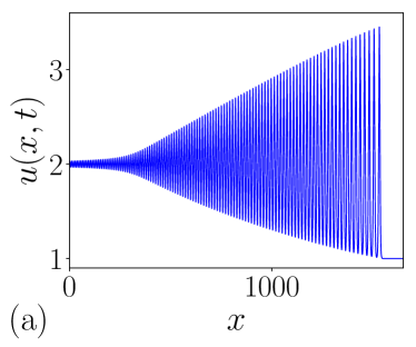
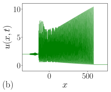
Figure 4. Conduit DSW stability determined by the value of $u_{+}/u_{-}$. a) Stable DSW with $u_{+}=1,u_{-}=2$ so that $u_{+}/u_{-}=1/2>5/32$; b) Unstable, imploded DSW with $u_{+}=0.15,u_{-}=2$ so that $u_{+}/u_{-}<5/32$.

We now compare the predictions of the (H)NLS analysis for the conduit DSW modulation with direct numerical simulations within the admissible range of Riemann data with $u_{+}/u_{-}>5/32$ that produces a stable DSW. Within this region, $\beta<0$ so the DSW orientation $d=+1$, and the harmonic edge is the trailing one, see Fig. 4. The coefficients $\delta$, $\lambda$, $\mu$ in the conduit-HNLS equation (24) and the coefficient $b_{2}$ in the second order expansions of the mean flow ${\overline{u}}$ are derived using symbolic computations in Mathematica as presented in Appendix A (see formulae (57)).

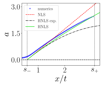
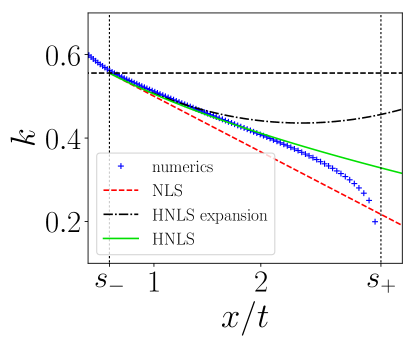
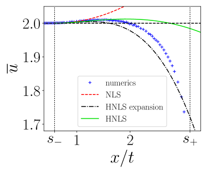
Figure 5. Amplitude, wavenumber, and mean field profiles for the conduit Riemann problem with $(u_{-},u_{+})=(2,1)$ at $t=500$ (blue pluses), the NLS/HNLS asymptotic descriptions given by (i) expansions (31) with the first order (NLS) approximation (dashed red line) and the second order (HNLS) approximation (dash-dotted black line) and (ii) the exact simple wave solution Eqs. (28), (29) of the dispersionless HNLS equation with coefficients (43), (57) (solid green line). The horizontal black dashed lines correspond to the values of the corresponding fields in the harmonic limit: $a=0$, $k=k_{-}\simeq 0.56$ and ${\overline{u}}=u_{-}=2$.

The comparisons between the dispersionless HNLS vacuum rarefaction simple wave solution (28), (29) with coefficients (43), (57), its asymptotic expansions (22), (31) and the numerical solution of the Riemann problem for the conduit equation are shown in Fig. 5. As in the previous cases, the full simple wave solution exhibits very good agreement with the direct numerical solution over a broad DSW region, while the first- and second-order approximations work satisfactorily only in a relatively narrow vicinity of the harmonic edge.

5.3. Serre equations

The presentation until now has emphasized scalar dispersive hydrodynamic equations in the form (1). Our methodology, however, can be applied to systems of dispersive hydrodynamic equations. As an example, we now consider the Serre system modeling fully nonlinear shallow water waves [55, 58]

(45) $$\begin{split}&\eta_{t}+(\eta u)_{x}=0,\\ &u_{t}+uu_{x}+\eta_{x}=\frac{1}{\eta}\left(\frac{\eta^{3}}{3}\left[u_{xt}+uu_{xx}-(u_{x})^{2}\right]\right)_{x}\,.\end{split}$$

We defer technical calculations to Appendices B and C. Here $\eta$ is the total depth of the fluid and $u$ is the depth averaged horizontal velocity. The linear dispersion relation of (LABEL:serre) for small amplitude waves propagating on the background $(\eta_{0},u_{0})$ has the form

(46) $$\omega=\omega_{0}^{\pm}(k,u_{0},\eta_{0})=k\left(u_{0}\pm\sqrt{\frac{\eta_{0}}{1+\eta_{0}^{2}k^{2}/3}}\right).$$

We assume Riemann initial data for (LABEL:serre)

(47) $$\eta(x,0)=\begin{cases}\eta_{-}&x<0\\ \eta_{+}&x>0\end{cases},\quad u(x,0)=\begin{cases}u_{-}&x<0\\ u_{+}&x>0\end{cases}$$

subject to an additional constraint

(48) $$u_{+}-2\eta_{+}^{1/2}=u_{-}-2\eta_{-}^{1/2}$$

that ensures a simple wave, 2-DSW resolution of (47) corresponding to the fast ‘$+$’ mode in the dispersion relation (46) [18, 19]. Due to scaling and Galilean symmetries of (LABEL:serre), we can assume $\eta_{+}=1$, $u_{+}=0$.

While the Serre system (LABEL:serre) is not integrable, it satisfies the pre-requisites of the DSW fitting method except for the loss of genuine nonlinearity in a certain parameter regime, discussed further below. The corresponding analysis has been carried out in [18], demonstrating excellent agreement with direct numerical simulations. An implicit expression for the harmonic (trailing) edge wavenumber $k_{-}$ of a 2-DSW as a function of the Riemann data (47), obtained in [18] by integrating a bi-directional generalization of the ODE (9), has the form

(49) $$\begin{split}&\sqrt{\alpha}\Delta-\left(\frac{4-\alpha}{3}\right)^{21/10}\left(\frac{1+\alpha}{2}\right)^{2/5}=0,\\ &\hbox{where}\quad\alpha=\left(\frac{2+s_{-}}{\sqrt{\Delta}}-2\right)^{1/3}.\end{split}$$

Here, $\Delta=\eta_{-}/\eta_{+}$ and $s_{-}=\partial_{k}\omega_{0}^{+}(k_{-},u_{-},\eta_{-})$. The result (49) is valid as long as $\partial s_{-}/\partial\eta_{-}<0$ (DSW fitting admissibility [33]) leading to the condition $\Delta<\Delta_{c}\approx 1.43$ [18]. When $\Delta=\Delta_{c}$, the Whitham modulation system loses genuine nonlinearity at the trailing edge.

The multiple scales asymptotic expansion for the Serre equations (LABEL:serre) that lead to the NLS equation (12) are carried out in Appendix B. In these expansions, the envelopes of the small amplitude oscillations of $\eta(x,t)$ and $u(x,t)$ are proportional to each other:

(50) $$\begin{split}&\begin{pmatrix}\eta(x,t)\\ u(x,t)\end{pmatrix}=\begin{pmatrix}\eta_{0}\\ u_{0}\end{pmatrix}+\left[\begin{pmatrix}\tilde{A}(x,t)\\ \tilde{B}(x,t)\end{pmatrix}e^{i[kx-\omega_{0}^{+}(k,\eta_{0},u_{0})t]}+{\mathrm{c.c.}}\right],\\ &\text{where}\quad\tilde{B}(x,t)=\tilde{A}(x,t)/\sqrt{\eta_{0}+\eta_{0}^{3}k^{2}/3}.\end{split}$$

The coefficients of the NLS equation (12) for the envelope $\tilde{A}(x,t)$ are found to be:

(51) $$\begin{split}&\beta=-\frac{\eta_{0}^{3/2}\kappa}{2(1+\kappa^{2}/3)^{5/2}},\\ &\gamma=\frac{243+297\kappa^{2}+42\kappa^{4}+\kappa^{6}+\kappa^{8}}{4\eta_{0}^{5/2}\kappa(27+9\kappa^{2}+\kappa^{4})(1+\kappa^{2}/3)^{3/2}},\\ &b_{1,\eta}=-\frac{(9-\kappa^{2})(3+\kappa^{2})^{3}}{\eta_{0}\kappa^{2}(27+9\kappa^{2}+\kappa^{4})},\\ &b_{1,u}=-\frac{(3+2\kappa^{2})(27+6\kappa^{2}+\kappa^{4})}{\eta_{0}^{3/2}\kappa^{2}\sqrt{1+\kappa^{2}/3}(27+9\kappa^{2}+\kappa^{4})},\end{split}$$

where $\kappa=\eta_{0}k$. Here $b_{1,\eta},b_{1,u}$ are the coefficients in the mean flow expansions $\overline{\eta}=\eta_{0}+b_{1,\eta}\rho$ and ${\overline{u}}=u_{0}+b_{1,u}\rho$. The NLS equation for the component $\tilde{B}$ is obtained by combining the NLS equation for $\tilde{A}$ and the proportionality relation (50).

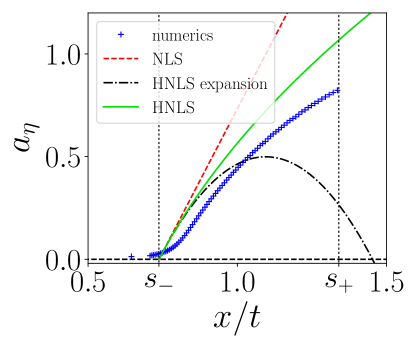
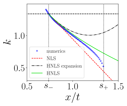
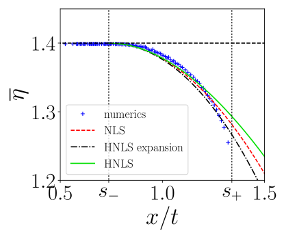
Figure 6. Amplitude, wavenumber, and mean field profiles for the Serre Riemann problem with $(\eta_{-},\eta_{+})=(1.4,1)$ and $(u_{-},u_{+})=(2\sqrt{\eta}_{-}-2,0)$. Comparison between direct numerical simulations at $t=800$ (blue pluses), the NLS/HNLS asymptotic descriptions given by (i) expansions (31) with the first order (NLS) approximation (dashed red line) and the second order (HNLS) approximation (dash-dotted black line) and (ii) the exact simple wave solution Eqs. (28), (29) of the dispersionless HNLS equation with coefficients (51), (74) and (75) (solid green line). The horizontal black dashed lines correspond to the values of the corresponding fields in the harmonic limit: $a_{\eta}=0$, $k=k_{-}\simeq 1.34$ and $\overline{\eta}=\eta_{-}=1.4$.

Going to $O(\varepsilon^{4})$, we obtain the coefficients $\delta,\lambda,\mu$ in the HNLS equation (24), as well as the coefficients $b_{2,\eta},b_{2,u}$ in the second order expansions of the mean flow $\overline{\eta}$, ${\overline{u}}$ in terms of $k,u_{0},\eta_{0}$. These are presented in Appendix C (see formulae (74) and (75)). In this higher order description, the envelopes $\tilde{A}$ and $\tilde{B}$ are no longer proportional to each other, and the coefficient $\mu$ in the HNLS equation has to be derived separately for each component.

To apply the HNLS equation to the description of the vicinity of the Serre DSW harmonic edge, we set $u_{0}=u_{-}$, $\eta_{0}=\eta_{-}$, $k=k_{-}$, where the dependence of $k_{-}$ on the Riemann data (47) is obtained numerically from the implicit equation (49).

The comparison between the simple wave solution (28),(29) with parameters given by (51), (74), (75) and the numerical solution of the Riemann problem for the Serre equations is displayed in Fig. 6. Also shown are the curves corresponding to the first order (22) and the second order (31) approximations of the full solution (28),(29). The comparisons are made for the DSW amplitude $a$, the wavenumber $k$ and the mean depth $\overline{\eta}$. We can see that the full simple wave solution (28),(29) of the dispersionless HNLS equation provides a more accurate description of the DSW modulation than the first and second order approximations. Similar to the KdV case, the full simple wave solution of the dispersionless HNLS equation provides a good approximation of the nonlinear wave modulation over a significant portion of the DSW, well beyond the formal applicability of the small amplitude (H)NLS approximation. On the other hand, we can see that, in contrast to the KdV case, the second order approximation (31) develops quite strong deviation from the actual modulation for moderate values of $(x/t-s_{-})$.

The final comment concerns the already discussed generic discrepancy between the simple wave modulation DSW solution and direct numerical solution of the Riemann problem in the vicinity of the harmonic edge (see the discussion at the end of Sec. 5.1). This discrepancy is more pronounced for the Serre equations than for the KdV equation although the overall agreement with the dispersionless HNLS solution is still quite good.

6. Conclusion and Discussion

In this work, we have developed an efficient, universal approach for the analytical description of the interior structure of a dispersive shock wave (DSW) that extends the previously developed DSW fitting method [16] for the DSW edge speeds. The key element of the extension is the realization that the DSW modulation described by an expansion fan solution of the Whitham modulation equations can be universally approximated, in the vicinity of the weakly nonlinear harmonic edge, by a special vacuum rarefaction solution of the shallow water equations. The connection between the original dispersive hydrodynamics and the approximating shallow water system occurs via a long-wave, dispersionless limit of the NLS equation for weakly nonlinear, narrow-band Stokes waves, whose parameters are determined by DSW fitting when the NLS equation is of defocusing type. The NLS type (defocusing or focusing) determines DSW stability properties. The developed approach is particularly attractive for applications as it allows one to avoid a potentially complex, full Whitham modulation analysis of DSWs in favor of the more straighforward and standard NLS theory.

The efficacy of the developed approach is demonstrated by several representative examples including the KdV equation, the Serre shallow water equations and the viscous fluid conduit equation, the two latter systems being non-integrable. In all considered cases, it is shown that the inclusion of higher order terms in the NLS equation dramatically improves agreement between the approximate modulation solution and the numerical solution of the original dispersive Riemann problem. The proposed method has broad implications for DSW analysis in non-integrable systems, where exact methods based on the inverse scattering theory are not available. One interesting perspective is to use the NLS approximation for the analytical description of multiphase modulations that are symptomatic of DSW implosions (see [44] and Sec. 5.2 of this paper). In this context, the description will necessarily depend upon dispersive terms in the NLS equation, which do not play a role in the classical expansion fan DSW solutions considered in the present paper. Further, the improved DSW description in Sec. 4, based on the higher order NLS equation, provides a general mathematical framework for DSW analysis in systems with non-convex dispersion, which are currently under active investigation [21, 57]. We also envisage intriguing connections with the multisymplectic theory of universal dispersive deformations of the Whitham equations near coalescing characteristics, precisely the configuration that occurs at the DSW harmonic edge; see [50, 9] and references therein.

Probably the most appealing extension of the developed harmonic edge DSW structure theory would be to find its counterpart in the vicinity of the DSW soliton edge (utilizing small $k$ asymptotics), and to construct a universal, matched, uniformly valid asymptotic solution for the entire DSW modulation.

Appendix A Derivation of the HNLS equation for the conduit equation

The derivation of the HNLS equation for KdV (32) is detailed in Ref. [8] and we simply repeat in this section the main steps of the derivation which are applicable to the conduit equation  (41). In order to derive the HNLS equation (24), we look for the solution of (41) in the form

(52) $$u=u_{0}+\varepsilon u_{1}+\varepsilon^{2}u_{2}+\varepsilon^{3}u_{3}+\dots$$

with

$$u_{1}=A(X,T_{1},T_{2},T_{3})e^{i(kx-\omega t)}+c.c,\ X=\varepsilon x,T_{1}=\varepsilon t,T_{2}=\varepsilon^{2}t,T_{3}=\varepsilon^{3}t.$$

The cancellation of the secular terms at $O(\varepsilon^{2})$ and $O(\varepsilon^{3})$ in the expansion in $\varepsilon$ gives Eqs. (11) and (12) respectively, and the cancellation of the secular term at $O(\varepsilon^{4})$ gives

(53) $$A_{T_{3}}+\delta A_{XXX}+\lambda|\tilde{A}|^{2}A_{X}+\mu A^{2}A^{*}_{X}=0,$$

As a by-product of the $O(\varepsilon^{4})$ expansion we also obtain a higher order correction of the mean ${\overline{u}}$ which reads:

(54) $${\overline{u}}-u_{0}\simeq\varepsilon^{2}b_{1}|A|^{2}+\varepsilon^{3}b_{2}i(AA_{X}^{*}-A^{*}A_{X}).$$

We define the un-scaled envelope $\tilde{A}(x,t)$ by:

(55) $$\tilde{A}(x,t)=\varepsilon A(\varepsilon x,\varepsilon t,\varepsilon^{2}t,\varepsilon^{3}t),$$

implying the new substitution rule (cf. Eq. (14)):

(56) $$\tilde{A}_{t}=\varepsilon^{2}A_{T_{1}}+\varepsilon^{3}A_{T_{2}}+\varepsilon^{4}A_{T_{3}}.$$

Combining Eqs. (11), (12), (53) with the substitution rule (56), we obtain the HNLS equation (24) for the un-scaled envelope $\tilde{A}(x,t)$.

Applying the above algorithm to the conduit equation (41) we find the coefficients of the HNLS equation (24) to be:

(57) $$\begin{split}&\delta=\frac{2u_{0}^{2}(1-6u_{0}k^{2}+u_{0}^{2}k^{4})}{(1+u_{0}k^{2})^{4}},\\ &\lambda=\frac{2(-9+9u_{0}k^{2}+21u_{0}^{2}k^{4}+23u_{0}^{3}k^{6}+8u_{0}^{4}k^{8})}{3u_{0}^{2}k^{2}(3+4u_{0}k^{2}+u_{0}^{2}k^{4})^{2}},\\ &\mu=\frac{-27+24u_{0}k^{2}+55u_{0}^{2}k^{4}+8u_{0}^{3}k^{6}}{3u_{0}^{2}k^{2}(1+u_{0}k^{2})(3+u_{0}k^{2})^{2}},\\ &b_{2}=\frac{2(3+2u_{0}k^{2}+7u_{0}^{2}k^{4})}{u_{0}^{2}k^{3}(3+u_{0}k^{2})^{2}}.\end{split}$$

Appendix B Derivation of the NLS equation for the Serre equations

We detail in this Appendix the multiple scales expansions for the Serre equations (LABEL:serre) leading to the NLS equation (12). Although the derivation of the NLS equation for systems is standard (see, e.g., [59]), the computation can be rather cumbersome because of the vectorial nature of the system; this difficulty can be overcome using symbolic computations, as we have done in this case (we used Mathematica). Similar to the multiple scales asymptotic expansions for scalar equations, we look for the solution in the form

(58) $$\Xi=\begin{pmatrix}\eta\\ u\end{pmatrix}=\begin{pmatrix}\eta_{0}\\ u_{0}\end{pmatrix}+\varepsilon\Xi_{1}+\varepsilon^{2}\Xi_{2}+\varepsilon^{3}\Xi_{3}+\dots$$

with

$$\Xi_{1}=\Psi(X,T_{1},T_{2})e^{i(kx-\omega t)}+c.c,\ X=\varepsilon x,T_{1}=\varepsilon t,T_{2}=\varepsilon^{2}t,$$

where $\Psi\in\mathbb{C}^{2}$ is a complex two-component vector. Substituting (58) into the Serre system (LABEL:serre) and collecting the $O(\varepsilon)$ terms we get

(59) $$M(ik,-i\omega)\Psi=0,$$

where

(60) $$M(ik,-i\omega)=\begin{pmatrix}i(u_{0}k-\omega)&i\eta_{0}k\\ ik&i(1+\eta_{0}^{2}k^{2}/3)(u_{0}k-\omega)\end{pmatrix}.$$

The null space of (60) is not empty if

(61) $$\omega=\omega_{0}^{\pm}(k,u_{0},\eta_{0})=k\left(u_{0}\pm\sqrt{\frac{\eta_{0}}{1+\eta_{0}^{2}k^{2}/3}}\right).$$

Eq. (61) is nothing but the linear dispersion relation (46) of the Serre system. The 2-DSW developing in the Riemann problem (LABEL:serre),(47),(48) corresponds to the fast ‘+’ mode (cf. Sec. 5.3 and [18, 19]) so we assume in the following that $\omega=\omega_{0}^{+}(k,\eta_{0},u_{0})$. Hence Eq. (59) yields the non trivial solution:

(62) $$\Psi=\Psi^{+}_{0}(X,T_{1},T_{2})=\begin{pmatrix}1\\ 1/\sqrt{\eta_{0}(1+\kappa^{2}/3)}\end{pmatrix}\,A(X,T_{1},T_{2}),$$

where $\kappa=\eta_{0}k$ is a convenient parameter and $A(X,T_{1},T_{2})$ is now a scalar. The kernel of $M^{T}$ is spanned by $\{L_{0}^{+},L^{-}\}$ where

(63) $$L_{0}^{\pm}=\left(\pm\sqrt{1+\kappa^{2}/3},\,\sqrt{\eta}_{0}\right)^{T}\,.$$

Assuming that $\Psi$ is given by (62) and $\omega=\omega_{0}^{+}(k,\eta_{0},u_{0})$, the second order of the asymptotic expansion reads

(64) $$M(\partial_{x},\partial_{t})\Xi_{2}=C_{1}e^{i(kx-\omega_{0}^{+}t)}+C_{2}e^{2i(kx-\omega_{0}^{+}t)}+{\mathrm{c.c.}},$$

where we drop the dependences of the dispersion relation $\omega_{0}^{+}$ by convenience. The vectors $C_{1}$ and $C_{2}$ are given by:

$$C_{1}=-\begin{pmatrix}\displaystyle A_{T_{1}}+\left(u_{0}+\sqrt{\frac{\eta_{0}}{1+\kappa^{2}/3}}\right)A_{X}\\ \displaystyle\sqrt{\frac{1+\kappa^{2}/3}{\eta_{0}}}A_{T_{1}}+\left(u_{0}\sqrt{\frac{\eta_{0}}{1+\kappa^{2}/3}}+\frac{3-\kappa^{2}}{3+\kappa^{2}}\right)A_{X}\end{pmatrix},$$

and

$$C_{2}=-\begin{pmatrix}\displaystyle\frac{2i\kappa}{\eta_{0}^{3/2}\sqrt{1+\kappa^{2}/3}}\,A^{2}\\ \displaystyle\frac{i\kappa(3-5\kappa^{2})}{\eta_{0}^{2}(3+\kappa^{2})}\,A^{2}\end{pmatrix}.$$

Since $\det M(ik,-i\omega_{0}^{+})=0$, a compatibility condition is necessary to solve Eq. (64) (cf. for instance Ref. [59]), thus we impose the ortogonality requirement $L_{0}^{+}\cdot C_{1}=0$. This condition is satisfied if the wave packet propagates with the group velocity $\partial_{k}\omega_{0}^{+}(k,\eta_{0},u_{0})$:

(65) $$A_{T_{1}}+\partial_{k}\omega_{0}^{+}(k,\eta_{0},u_{0})\,A_{X}=0.$$

Providing that (65) is respected, one solution of (64) is:

(66) $$\begin{split}\Xi_{2}=\begin{pmatrix}Q\\ R\end{pmatrix}&+\left[\begin{pmatrix}0\\ \displaystyle\frac{i\sqrt{3\eta_{0}}\kappa}{(3+\kappa^{2})^{3/2}}\end{pmatrix}A_{X}e^{i(kx-\omega_{0}^{+}t)}+{\mathrm{c.c.}}\right]\\ &+\left[\begin{pmatrix}\displaystyle\frac{3+\kappa^{2}}{2\eta_{0}\kappa^{2}}\\ \displaystyle\frac{3-\kappa^{2}}{2\eta_{0}^{3/2}\kappa^{2}\sqrt{1+\kappa^{2}/3}}\end{pmatrix}A^{2}e^{2i(kx-\omega_{0}^{+}t)}+{\mathrm{c.c.}}\right],\end{split}$$

where $Q(X,T_{1},T_{2})$ and $R(X,T_{1},T_{2})$ are two unknown fields that remain to be determined. $Q$ and $R$ are necessary for the consistency of the asymptotic expansion, as we shall see at the next order (cf. Eqs. (68)).

The solution (66) is not unique and the general solution of (64) reads as: $\Xi_{2}+\left[K(X,T_{1},T_{2})e^{i(kx-\omega_{0}^{+}t)}+{\mathrm{c.c.}}\right]$ where $K(X,T_{1},T_{2})$ belongs to the kernel of $M(ik,-i\omega_{0}^{+})$. This additional term does not modify the NLS equation (12) in the end but it plays an important role in higher order descriptions (cf. Appendix C). In practice, we choose $K(X,T_{1},T_{2})$ such that one of the two components of $\Xi_{2}$ proportional to $e^{i(kx-\omega_{0}^{+}t)}$ is equal to $0$ (which is already the case here).

Finally, if we substitute $\Xi_{2}$ by the solution (66), the $O(\varepsilon^{3})$ of the expansion reads

(67) $$M(\partial_{x},\partial_{t})\Xi_{3}=D_{0}+[D_{1}e^{i(kx-\omega_{0}^{+}t)}+D_{2}e^{2i(kx-\omega_{0}^{+}t)}+D_{3}e^{3i(kx-\omega_{0}^{+}t)}+{\mathrm{c.c.}}],$$

with

$$D_{0}=-\begin{pmatrix}\displaystyle Q_{T_{1}}+u_{0}Q_{X}+\eta_{0}R_{X}+\frac{(|A|^{2})_{X}}{\sqrt{\eta_{0}(1+\kappa^{2}/3)}}\\ \displaystyle R_{T_{1}}+Q_{X}+u_{0}R_{X}+\frac{9+6\kappa^{2}-\kappa^{4}}{\eta_{0}(3+\kappa^{2})^{2}}(|A|^{2})_{X}\end{pmatrix},$$

and

$$\begin{split}D_{1}=\;&-\begin{pmatrix}\displaystyle A_{T_{2}}+\frac{i\sqrt{3}\eta_{0}^{3/2}\kappa}{(3+\kappa^{2})^{3/2}}A_{XX}+\frac{3i}{\eta_{0}^{5/2}\kappa\sqrt{1+\kappa^{2}/3}}|A|^{2}A\\ \displaystyle\sqrt{\frac{1+\kappa^{2}/3}{\eta_{0}}}A_{T_{2}}+\frac{i\eta_{0}\kappa(6-\kappa^{2})}{(3+\kappa^{2})^{2}}A_{XX}+\frac{i(9+7\kappa^{4})}{2\eta_{0}^{3}\kappa(3+\kappa^{2})}|A|^{2}A\end{pmatrix}\\ &-\begin{pmatrix}\displaystyle\frac{i\kappa}{\eta_{0}^{3/2}\sqrt{1+\kappa^{2}/3}}QA+\frac{i\kappa}{\eta_{0}}RA\\ \displaystyle\frac{-2i\kappa^{3}}{\eta_{0}^{2}(3+\kappa^{2})}QA+\frac{i\kappa\sqrt{1+\kappa^{2}/3}}{\eta_{0}^{3/2}}RA\end{pmatrix}.\end{split}$$

We do not present the coefficients $D_{2}$ and $D_{3}$ for the second and third harmonic terms at this stage since they are not needed for the derivation of the NLS equation. However, these terms are needed to solve (67), and ultimately derive the HNLS equation at the next order.

Since $M(0,0)=0$, the constant term $D_{0}$ should be equal to $0$. This condition is respected for $Q(X,T_{1},T_{2})$ and $R(X,T_{1},T_{2})$ given by:

(68) $$\begin{split}&Q=-\frac{(9-\kappa^{2})(3+\kappa^{2})^{3}}{\eta_{0}\kappa^{2}(27+9\kappa^{2}+\kappa^{4})}|A|^{2},\\ &R=-\frac{(3+2\kappa^{2})(27+6\kappa^{2}+\kappa^{4})}{\eta_{0}^{3/2}\kappa^{2}\sqrt{1+\kappa^{2}/3}(27+9\kappa^{2}+\kappa^{4})}|A|^{2}.\end{split}$$

Providing that $Q$ and $R$ are substituted by the solutions (68), the compatibility condition $L_{0}^{+}\cdot D_{1}=0$ gives

(69) $$iA_{T_{2}}+\beta(k)A_{XX}+\gamma(k)|A|^{2}A=0,$$

with

$$\beta=-\frac{\eta_{0}^{3/2}\kappa}{2(1+\kappa^{2}/3)^{5/2}},\;\gamma=\frac{243+297\kappa^{2}+42\kappa^{4}+\kappa^{6}+\kappa^{8}}{4\eta_{0}^{5/2}\kappa(27+9\kappa^{2}+\kappa^{4})(1+\kappa^{2}/3)^{3/2}}.$$

Appendix C Derivation of the HNLS equation for the Serre equations

The definition of the un-scaled envelope (55) is not always adequate for systems. Unlike scalar equations where the only term of the solution $u(x,t)$ proportional to the first harmonic $e^{i(kx-\omega t)}$ is $\varepsilon A(X,T_{1},T_{2})$, solutions of “multi-component” systems (Eq. (LABEL:serre) for instance) can contain higher order corrections of the envelope.

For the Serre system (LABEL:serre) we define (cf. Appendix. B):

(70) $$\begin{pmatrix}\eta(x,t)\\ u(x,t)\end{pmatrix}=\begin{pmatrix}\eta_{0}\\ u_{0}\end{pmatrix}+\left[\begin{pmatrix}\tilde{A}(x,t)\\ \tilde{B}(x,t)\end{pmatrix}e^{i(kx-\omega_{0}^{+}t)}+{\mathrm{c.c.}}\right].$$

We have shown in the previous section, cf. Eqs. (62) and (66), that

(71) $$\begin{pmatrix}\tilde{A}(x,t)\\ \tilde{B}(x,t)\end{pmatrix}=\begin{pmatrix}\varepsilon A(X,T_{1},T_{2},T_{3})\\ \varepsilon\alpha A(X,T_{1},T_{2},T_{3})+i\varepsilon^{2}\sigma A_{X}(X,T_{1},T_{2},T_{3})\end{pmatrix},$$

with $\alpha=1/\sqrt{\eta_{0}(1+\eta_{0}^{2}k^{2}/3)}$ and $\sigma=\sqrt{3\eta_{0}}\eta_{0}k/(3+\eta_{0}^{2}k^{2})^{3/2}$. Definition (55) and the substitution rule (56) still hold for the component $\tilde{A}$ for which we obtain Eq. (24). However, a new substitution rule is necessary to derive the modulation equation for the “total amplitude” $\tilde{B}$:

(72) $$\tilde{B}_{t}=\varepsilon^{2}\alpha A_{T_{1}}+\varepsilon^{3}\alpha A_{T_{2}}+\varepsilon^{4}\alpha A_{T_{3}}+i\varepsilon^{3}\alpha A_{XT_{1}}+i\varepsilon^{4}\alpha A_{XT_{2}}.$$

A careful derivation gives (cf. Ref. [54]):

(73) $$\begin{split}&i\tilde{B}_{t}+i\omega_{0}^{\prime}(k)B_{x}+\beta\tilde{B}_{xx}+\frac{\gamma}{\alpha^{2}}|\tilde{B}|^{2}\tilde{B}+i\delta\tilde{B}_{xxx}+i\frac{\lambda}{\alpha^{2}}|B|^{2}\tilde{B}_{x}\\ &+i\left(\frac{\mu}{\alpha^{2}}+\frac{2\gamma\sigma}{\alpha^{3}}\right)\tilde{B}^{2}\tilde{B}^{*}_{x}=0.\end{split}$$

We notice that the coefficient in front of $\tilde{B}^{2}\tilde{B}^{*}_{x}$ in (73) is not proportional to $\mu$ as one might expect if one considered the inadequate definition $\tilde{B}=\varepsilon\alpha A$. Nonetheless, to the first order both $\tilde{B}=\varepsilon\alpha A$ and definition (71) yield the same NLS equation for $\tilde{B}$ which can be simply obtained by substituting in (15) $\tilde{A}$ by $\tilde{B}/\alpha$.

We now present, without derivation, the coefficients for the HNLS equation (24) describing the envelope $\tilde{A}$ for the component $\eta(x,t)$ of the Serre system. The envelope $\tilde{B}$ of the component $u(x,t)$ can be put in the form (71) allowing for the determination the corresponding coefficient $\sigma$. The coefficients computed using Mathematica are:

(74) $$\begin{split}&\delta=\frac{3\sqrt{3}\eta_{0}^{5/2}(3-4\kappa^{2})}{2(3+\kappa^{2})^{7/2}},\\ &\begin{split}\lambda=\;&(9-\kappa^{2})(-2187-3159\kappa^{2}-567\kappa^{4}+243\kappa^{6}+90\kappa^{8}\\ &+8\kappa^{10})/(6\eta_{0}^{3/2}\kappa^{2}(1+\kappa^{2}/3)^{5/2}(27+9\kappa^{2}+\kappa^{4})^{2}),\end{split}\\ &\begin{split}\mu=\;&(-19683-24786\kappa^{2}-11502\kappa^{4}-2754\kappa^{6}-276\kappa^{8}+14\kappa^{10}\\ &+3\kappa^{12})/(4\eta_{0}^{3/2}\kappa^{2}(1+\kappa^{2}/3)^{5/2}(27+9\kappa^{2}+\kappa^{4})^{2}),\end{split}\\ &\sigma=\frac{\sqrt{3\eta_{0}}\kappa}{(3+\kappa^{2})^{3/2}},\end{split}$$

(75) $$\begin{split}&b_{2,\eta}=\frac{6(3+\kappa^{2})(243+81\kappa^{2}+36\kappa^{4}+4\kappa^{6})}{\kappa^{3}(27+9\kappa^{2}+\kappa^{4})^{2}},\\ &\begin{split}b_{2,u}=&\sqrt{3}(13122+15309\kappa^{2}+8505\kappa^{4}+2322\kappa^{6}+315\kappa^{8}+27\kappa^{10}\\ &+2\kappa^{12})/(\sqrt{\eta}_{0}\kappa^{3}(3+\kappa^{2})^{3/2}(27+9\kappa^{2}+\kappa^{4})^{2}),\end{split}\end{split}$$

where $\kappa=\eta_{0}k$.

Appendix D Numerical Methods

The initial step (3) of the Riemann problem is implemented numerically by the function:

(76) $$u(x,t=0)=\frac{u_{+}-u_{-}}{2}\tanh\left(\frac{x}{\xi}\right)+\frac{u_{+}+u_{-}}{2},$$

for the KdV  (32) and the conduit  (41) equations. We implement a similar step for the field $\eta(x,t)$ in the Serre system (LABEL:serre). We shall use $\xi=2$ in our examples. We choose periodic boundary conditions: $u(x+L)=u(x)$ (and $\eta(x+L)=\eta(x)$); in practice we consider a domain $[0;L]$ sufficiently large to avoid interactions with the boundaries.

We used a spectral method to solve the Riemann problem for the KdV equation (cf. for instance Ref. [61]): we rewrite Eq. (32) in the form

(77) $$(e^{-ik^{3}t}\hat{u})_{t}+\,\frac{ik}{2}\widehat{u^{2}}=0,$$

where $\hat{u}$ and $\widehat{u^{2}}$ are spatial Fourier transforms of $u$ and $u^{2}$ respectively. The time integration of (77) is performed through the 4th order explicit Runge-Kutta method and in order to diminish the aliasing error we consider the “Orszag 2/3 rule” [48].

In order to solve the Riemann problem for the conduit equation, we rewrite (41) in the following form (cf. for instance Ref. [45]):

(78) $$uw+2uu_{x}-(u^{2}w_{x})_{x}=0,$$

(79) $$u_{t}=wu.$$

Derivatives in (78) are approximated using centered finite differences; then $w(x,t)$ is obtained by inverting the corresponding banded linear system. (79) is integrated through the 4th order explicit Runge-Kutta method.

Similarly we rewrite the Serre system (41) in the form:

(80) $$w+uu_{x}+\eta_{x}=\frac{1}{\eta}\left(\frac{\eta^{3}}{3}\left[w_{x}+uu_{xx}-(u_{x})^{2}\right]\right)_{x},$$

(81) $$\eta_{t}+(\eta u)_{x}=0,\quad u_{t}=w,$$

and apply the same algorithm.

References

- [1] M. J. Ablowitz. Nonlinear Dispersive Waves: Asymptotic Analysis and Solitons. Cambridge Texts in Applied Mathematics. Cambridge University Press, Cambridge, UK ; New York, 1 edition, 2011.
- [2] X. An, T. R. Marchant, and N. F. Smyth. Dispersive shock waves governed by the Whitham equation and their stability. Proc. R. Soc. A, 474(2216):20180278, Aug. 2018.
- [3] D. Arcas and H. Segur. Seismically generated tsunamis. Philosophical Transactions of the Royal Society A: Mathematical, Physical and Engineering Sciences, 370:1505–1542, 2012.
- [4] T. B. Benjamin, J. L. Bona, and J. J. Mahony. Model Equations for Long Waves in Nonlinear Dispersive Systems. Philosophical Transactions of the Royal Society of London. Series A, Mathematical and Physical Sciences, 272(1220):47–78, 1972.
- [5] D. J. Benney and A. C. Newell. Propagation of nonlinear wave envelopes. Journal of Mathematics and Physics, 46(2):133–139, 1967.
- [6] P. L. Bhatnagar. Nonlinear Waves in One-Dimensional Dispersive Systems. Oxford University Press, New York, Dec. 1980.
- [7] G. Biondini, G. El, M. Hoefer, and P. Miller. Dispersive hydrodynamics: Preface. Physica D, 333:1–5, Oct. 2016.
- [8] J. P. Boyd and G.-Y. Chen. Weakly nonlinear wavepackets in the Korteweg-de Vries equation: the KdV/NLS connection. Mathematics and Computers in Simulation, 55(4):317–328, Mar. 2001.
- [9] T. J. Bridges. Symmetry, Phase Modulation and Nonlinear Waves. Cambridge University Press, Cambridge, 2017.
- [10] D. R. Christie. The morning glory of the Gulf of Carpentaria: a paradigm for non-linear waves in the lower atmosphere. Austral. Met. Mag., 41:21–60, 1992.
- [11] C. Conti, A. Fratalocchi, M. Peccianti, G. Ruocco, and S. Trillo. Observation of a Gradient catastrophe generating solitons. Phys. Rev. Lett., 102(8):083902, 2009.
- [12] M. Crosta, S. Trillo, and A. Fratalocchi. The Whitham approach to dispersive shocks in systems with cubic -quintic nonlinearities. New Journal of Physics, 14(9):093019, Sept. 2012.
- [13] Z. Dutton, M. Budde, C. Slowe, and L. V. Hau. Observation of quantum shock waves created with ultra-compressed slow light pulses in a Bose-Einstein condensate. Science, 293:663, 2001.
- [14] I. Egorova, Z. Gladka, V. Kotlyarov, and G. Teschl. Long-time asymptotics for the Korteweg-de Vries equation with step-like initial data. Nonlinearity, 26:1839–1864, 2013.
- [15] G. El, M. Hoefer, and M. Shearer. Dispersive and diffusive-dispersive shock waves for nonconvex conservation laws. SIAM Rev., 59:3–61, 2017.
- [16] G. A. El. Resolution of a shock in hyperbolic systems modified by weak dispersion. Chaos, 15:037103, 2005.
- [17] G. A. El, A. Gammal, E. G. Khamis, R. A. Kraenkel, and A. M. Kamchatnov. Theory of optical dispersive shock waves in photorefractive media. Phys. Rev. A, 76(5):053813, 2007.
- [18] G. A. El, R. H. J. Grimshaw, and N. F. Smyth. Unsteady undular bores in fully nonlinear shallow-water theory. Phys. Fluids, 18(2):027104–17, 2006.
- [19] G. A. El and M. A. Hoefer. Dispersive shock waves and modulation theory. Physica D, 333:11–65, 2016.
- [20] G. A. El, V. V. Khodorovskii, and A. V. Tyurina. Undular bore transition in bi-directional conservative wave dynamics. Physica D, 206(3-4):232–251, 2005.
- [21] G. A. El and N. F. Smyth. Radiating dispersive shock waves in non-local optical media. Proc. R. Soc. A, 472(2187):20150633, Mar. 2016.
- [22] J. G. Esler and J. D. Pearce. Dispersive dam-break and lock-exchange flows in a two-layer fluid. J. Fluid Mech., 667:555–585, 2011.
- [23] J. Fatome, C. Finot, G. Millot, A. Armaroli, and S. Trillo. Observation of optical undular bores in multiple four-wave mixing. Phys. Rev. X, 4(2):021022, May 2014.
- [24] H. Flaschka, M. G. Forest, and D. W. McLaughlin. Multiphase averaging and the inverse spectral solution of the Korteweg-de Vries equation. Comm. Pure Appl. Math., 33:739–784, 1980.
- [25] N. Ghofraniha, C. Conti, G. Ruocco, and S. Trillo. Shocks in nonlocal media. Phys. Rev. Lett., 99:043903, 2007.
- [26] T. Grava and C. Klein. Numerical solution of the small dispersion limit of Korteweg - de Vries and Whitham equations. Comm. Pure Appl. Math., 60(11):1623–1664, 2007.
- [27] R. Grimshaw and K. Helfrich. Long-time solutions of the Ostrovsky equation. Stud. Appl. Math., 121(1):71–88, July 2008.
- [28] R. Grimshaw and C. Yuan. Depression and elevation tsunami waves in the framework of the Korteweg -de Vries equation. Natural Hazards, Sept. 2016.
- [29] R. Grimshaw and C. Yuan. Internal undular bores in the coastal ocean, in: M. G. Velarde, R. Yu. Tarakanov, and A. V. Marchenko, Ocean in Motion, Springer Oceanography. Springer, 2018.
- [30] E. Gromov and V. Talanov. Nonlinear dynamics of short wave trains in dispersive media. JETP, 83:73–79, 1996.
- [31] A. V. Gurevich, A. L. Krylov, and G. A. El. Nonlinear modulated waves in dispersive hydrodynamics. Sov. Phys. JETP, 71(5):899–910, 1990.
- [32] A. V. Gurevich and L. P. Pitaevskii. Nonstationary structure of a collisionless shock wave. Sov. Phys. JETP, 38(2):291–297, 1974. Translation from Russian of A. V. Gurevich and L. P. Pitaevskii, Zh. Eksp. Teor. Fiz. 65, 590-604 (August 1973).
- [33] M. A. Hoefer. Shock waves in dispersive Eulerian fluids. J. Nonlin. Sci., 24(3):525–577, 2014.
- [34] M. A. Hoefer, M. J. Ablowitz, I. Coddington, E. A. Cornell, P. Engels, and V. Schweikhard. Dispersive and classical shock waves in Bose-Einstein condensates and gas dynamics. Phys. Rev. A, 74:023623, 2006.
- [35] M. A. Hoefer, G. A. El, and A. M. Kamchatnov. Oblique spatial dispersive shock waves in nonlinear Schrödinger flows. SIAM J. Appl. Math., 77:1352–1374, 2017.
- [36] M. A. Hoefer, P. Engels, and J. Chang. Matter-wave interference in Bose-Einstein condensates: A dispersive hydrodynamic perspective. Physica D, 238(15):1311–1320, 2009.
- [37] P. P. Janantha, P. Sprenger, M. Hoefer, and M. Wu. Observation of self-cavitating envelope dispersive shock waves in yttrium iron garnet thin films. Phys. Rev. Lett., 119, 2017.
- [38] R. Jenkins. Regularization of a sharp shock by the defocusing nonlinear Schrödinger equation. Nonlinearity, 28:2131, 2015.
- [39] A. M. Kamchatnov. Nonlinear periodic waves and their modulations: an introductory course. World Scientific, 2000.
- [40] Y. Kodama. Optical solitons in a monomode fiber. J Stat Phys, 39(5-6):597–614, June 1985.
- [41] Y. Kodama and A. Hasegawa. Nonlinear pulse propagation in a monomode dielectric guide. IEEE J. Quantum Electronics, 23:510–524, 1987.
- [42] Y. Kodama, V. U. Pierce, and F.-R. Tian. On the Whitham Equations for the Defocusing Complex Modified KdV Equation. SIAM Journal on Mathematical Analysis, 40(5):1750–1782, Jan. 2009.
- [43] P. D. Lax. Hyperbolic systems of conservation laws and the mathematical theory of shock waves. SIAM, Philadelphia, PA, 1973.
- [44] N. K. Lowman and M. A. Hoefer. Dispersive shock waves in viscously deformable media. J. Fluid Mech., 718:524–557, 2013.
- [45] M. D. Maiden and M. A. Hoefer. Modulations of viscous fluid conduit periodic waves. Proc. R. Soc. A, 472(2196):20160533, 2016.
- [46] M. D. Maiden, N. K. Lowman, D. V. Anderson, M. E. Schubert, and M. A. Hoefer. Observation of dispersive shock waves, solitons, and their interactions in viscous fluid conduits. Phys. Rev. Lett., 116(17):174501, 2016.
- [47] A. Newell. Solitons in Mathematics and Physics. CBMS-NSF Regional Conference Series in Applied Mathematics. Society for Industrial and Applied Mathematics, 1985.
- [48] S. A. Orszag, Comparison of pseudospectral and spectral approximations, Stud. Appl. Math., 51:253–259, 1972.
- [49] A. Porter and N. F. Smyth. Modeling the Morning Glory of the Gulf of Carpentaria. J. Fluid Mech., 454(-1):1–20, 2002.
- [50] D. J. Ratliff and T. J. Bridges. Whitham modulation equations, coalescing characteristics, and dispersive Boussinesq dynamics. Physica D, 333:107–116, Oct. 2016.
- [51] E. Rolley, C. Guthmann, and M. S. Pettersen. The hydraulic jump and ripples in liquid helium. Physica B: Condensed Matter, 394(1):46–55, 2007.
- [52] D. R. Scott, D. J. Stevenson, and J. A. Whitehead. Observations of solitary waves in a viscously deformable pipe. Nature, 319(6056):759–761, Feb. 1986.
- [53] A. Scotti. Observation of very large and steep internal waves of elevation near the Massachusetts coast. Geophys. Res. Lett., 31(22), 2004.
- [54] Y. V. Sedletsky. The fourth-order nonlinear Schrödinger equation for the envelope of Stokes waves on the surface of a finite-depth fluid. JETP, 97(1):180–193, 2003.
- [55] F. Serre. Contribution l’étude des coulements permanents et variables dans les canaux. La Houille Blanche, (3, 6):374–388, 830–872, Dec. 1953.
- [56] N. F. Smyth and P. E. Holloway. Hydraulic jump and undular bore formation on a shelf break. J. Phys. Oceanogr., 18(7):947–962, 1988.
- [57] P. Sprenger and M. Hoefer. Shock waves in dispersive hydrodynamics with nonconvex dispersion. SIAM J. Appl. Math., 77:26–50, 2017.
- [58] C. H. Su and C. S. Gardner. Korteweg‐de Vries Equation and Generalizations. III. Derivation of the Korteweg - de Vries Equation and Burgers Equation. J. Math. Phys., 10(3):536–539, Mar. 1969.
- [59] T. Taniuti and N. Yajima. Perturbation Method for a Nonlinear Wave Modulation. I. J. Math. Phys., 10(8):1369–1372, Aug. 1969.
- [60] M. Tissier, P. Bonneton, F. Marche, F. Chazel, and D. Lannes. Nearshore dynamics of tsunami-like undular bores using a fully nonlinear Boussinesq model. J. Coast. Eng. , SI 64, 2011.
- [61] L. N. Trefethen. Spectral Methods in Matlab. SIAM: Society for Industrial and Applied Mathematics, 2001.
- [62] W. Wan, S. Jia, and J. W. Fleischer. Dispersive superfluid-like shock waves in nonlinear optics. Nat. Phys., 3(1):46–51, 2007.
- [63] G. B. Whitham. Non-linear dispersive waves. Proc. R. Soc. A, 283:238–261, 1965.
- [64] G. B. Whitham. Two-timing, variational principles and waves. J. Fluid Mech., 44(02):373, Nov. 1970.
- [65] G. B. Whitham. Linear and nonlinear waves. Wiley, New York, 1974.
- [66] G. Xu, M. Conforti, A. Kudlinski, A. Mussot, and S. Trillo. Dispersive dam-break flow of a photon fluid. Phys. Rev. Lett., 118(25):254101, June 2017.
- [67] J. Yang. Nonlinear Waves in Integrable and Non-integrable Systems. Mathematical Modeling and Computation. Society for Industrial and Applied Mathematics, 2010.