Signature change in matrix model solutions

A. Stern and Chuang Xu

ABSTRACT

Various classical solutions to lower dimensional IKKT-like Lorentzian matrix models are examined in their commutative limit. Poisson manifolds emerge in this limit, and their associated induced and effective metrics are computed. Signature change is found to be a common feature of these manifolds when quadratic and cubic terms are included in the bosonic action. In fact, a single manifold may exhibit multiple signature changes. Regions with Lorentzian signature may serve as toy models for cosmological space-times, complete with cosmological singularities, occurring at the signature change. The singularities are resolved away from the commutative limit. Toy models of open and closed cosmological space-times are given in two and four dimensions. The four dimensional cosmologies are constructed from non-commutative complex projective spaces, and they are found to display a rapid expansion near the initial singularity.

1 Introduction

Signature change is believed to be a feature of quantum gravity.[1]-[10] It has been discussed in the context of string theory,[6] loop quantum gravity,[7],[10] and causal dynamical triangulation[8]. Recently, signature change has also been shown to result from for certain solutions to matrix equations.[11],[12],[13] These are the classical equations of motion that follow from Ishibashi, Kawai, Kitazawa and Tsuchiya (IKKT)-type models,[14] with a Lorentzian background target metric. The signature change occurs in the induced metrics of the continuous manifolds that emerge upon taking the commutative (or equivalently, continuum or semi-classical) limits of the matrix model solutions. Actually, as argued by Steinacker, the relevant metric for these emergent manifolds is not, in general, the induced metric, but rather, it is the metric that appears upon the coupling to matter.[15] The latter is the so-called effective metric of the emergent manifold, and it is determined from the symplectic structure that appears in the commutative limit, as well as the induced metric. Signature changes also occur for the effective metric of these manifolds, and in fact, they precisely coincide with the signature changes in the induced metric. The signature changes in the induced or effective metric correspond to singularities in the curvature tensor constructed from these metrics. The singularities are resolved away from the commutative limit, where the description of the solution is in terms of representations of some matrix algebras.

As well as being of intrinsic interest, signature changing matrix model solutions could prove useful for cosmology. It has been shown that toy cosmological models can be constructed for regions of the manifolds where the metric has Lorentzian signature. These regions can represent both open and closed cosmologies, complete with cosmological singularities which occur at the signature changes. As stated above such singularities are resolved away from the commutative limit. Furthermore, in [13], a rapid expansion, although not exponential, was found to occur immediately after the big bang singularity.

The previous examples of matrix models where signature change was observed include the fuzzy sphere embedded in a three-dimensional Lorentzian background,[11] fuzzy $CP^{2}$ in an eight-dimensional Lorentzian background,[12] and non-commutative $H^{4}$ in ten-dimensional Lorentz space-time.[13] For the purpose of examining signature changes, it is sufficient to restrict to the bosonic sector of the matrix models. In this article we present multiple additional examples of solutions to bosonic matrix models that exhibit signature change. We argue that signature change is actually a common feature of solutions to IKKT-type matrix models with indefinite background metric, in particular, when mass terms are included in the matrix model action. (Mass terms have been shown to result from an IR regularization.[16]) In fact, a single solution can exhibit multiple signature changes. As an aside, it is known that there are zero mean curvature surfaces in three-dimensional Minkowski space that change from being space-like to being time-like.[17]-[21] The signature changing surfaces that emerge from solutions to the Lorentzian matrix models studied here do not have zero mean curvature.

As a warm up, we review two-dimensional solutions to the three-dimensional Lorentz matrix model, consisting of a quartic (Yang-Mills) and a cubic term, and without a quadratic (mass) term. Known solutions are non-commutative $(A)dS^{2}$[22]-[26] and the non-commutative cylinder.[27],[28],[29] They lead to a fixed signature upon taking the commutative limit. New solutions appear when the quadratic term is included in the action. These new solutions exhibit signature change. One such solution, found previously, is the Lorentzian fuzzy sphere.[11] Others can be constructed by deforming the non-commutative $AdS^{2}$ solution. After taking the commutative limit of these matrix solutions, one finds regions of the emergent manifolds where the metric has Lorentzian signature. In the case of the Lorentzian fuzzy sphere, the Lorentzian region crudely describes a two-dimensional closed cosmology, complete with an initial and final singularity. In the case of the deformation of non-commutative (Euclidean) $(A)dS^{2}$, the Lorentzian region describes a two-dimensional open cosmology.

Natural extensions of these solutions to higher dimensions are the non-commutative complex projective spaces.[30]-[36] Since we wish to recover noncompact manifolds, as well as compact manifolds in the commutative limit, we should consider the indefinite versions of these non-commutative spaces,[37] as well as those constructed from compact groups. For four dimensional solutions, there are then three such candidates: non-commutative $CP^{2}$, $CP^{1,1}$ and $CP^{0,2}$. The latter two solve an eight-dimensional (massless) matrix model with indefinite background metric, specifically, the $su(2,1)$ Cartan-Killing metric. These solutions give a fixed signature after taking the commutative limit. So as with the previous examples, the massless matrix model yields no signature change. Once again, new solutions appear when a mass term is included, and they exhibit signature change, possibly multiple signature changes. These solutions include deformations of non-commutative $CP^{2}$, $CP^{1,1}$ and $CP^{0,2}$. A deformed non-commutative $CP^{0,2}$ solution can undergo two signature changes, while a deformed non-commutative $CP^{2}$ solution can have up to three signature changes. Upon taking the commutative limit, the deformed non-commutative $CP^{1,1}$ and $CP^{0,2}$ solutions have regions with Lorentzian signature that describe expanding open space-time cosmologies, complete with a big bang singularity occurring at the signature change. The commutative limit of the deformed non-commutative $CP^{2}$ solution has a region with Lorentzian signature that describes a closed space-time cosmology, complete with initial/final singularities. Like the non-commutative $H^{4}$ solution found in [13], these solutions display extremely rapid expansion near the cosmological singularities. Also as in [13], the space-times emerging from the deformed non-commutative $CP^{1,1}$ and $CP^{0,2}$ solutions expand linearly at late times. It suggests that these are universal properties of $4d$ signature changing solutions to IKKT-type matrix models.

The outline for this article is the following: In section two we review the non-commutative $(A)dS^{2}$ and cylinder solutions to the (massless) three-dimensional Lorentz matrix model. We include the mass term the matrix model action in section three, and examine the resulting signature changing matrix model solutions. The non-commutative $CP^{1,1}$ and $CP^{0,2}$ solutions to an eight-dimensional (massless) matrix model (in the semi-classical limit) are examined in section four. The mass term is added to the action in section five, and there we study the resulting deformed non-commutative $CP^{1,1}$, $CP^{0,2}$ and $CP^{2}$ solutions. In appendix A we list some properties of $su(2,1)$ in the defining representation. In appendix B we review a derivation of the effective metric, and compute it for the examples of $CP^{1,1}$ and $CP^{0,2}$.

2 Three-dimensional Lorentzian matrix model

We begin by considering the bosonic sector of the three-dimensional Lorentzian matrix model with an action consisting of a quartic (Yang-Mills) term and a cubic term:

$$S(X)=\frac{1}{{\tt g}^{2}}{\rm Tr}\Bigl{(}-\frac{1}{4}[X_{\mu},X_{\nu}][X^{\mu},X^{\nu}]+\frac{i}{3}a\,\epsilon_{\mu\nu\lambda}X^{\mu}[X^{\nu},X^{\lambda}]\Bigr{)}\;$$ (2.1)

Here $X^{\mu},\;\mu=0,1,2$, are infinite-dimensional hermitean matrices and $a$ and ${\tt g}$ are constants. Tr denotes a trace, indices $\mu,\nu,\lambda,...$ are raised and lowered with the Lorentz metric $\eta_{\mu\nu}=$diag$(-,+,+)$, and the totally antisymmetric symbol $\epsilon_{\mu\nu\lambda}$ is defined such that $\epsilon_{012}=1$. Extremizing the action with respect to variations in $X^{\mu}$ leads to the classical equations of motion

$$[[X_{\mu},X_{\nu}],X^{\nu}]+ia\,\epsilon_{\mu\nu\lambda}[X^{\nu},X^{\lambda}]=0$$ (2.2)

The equations of motion (2.2) are invariant under:

i) unitary ‘gauge’ transformations, $X^{\mu}\rightarrow UX^{\mu}U^{\dagger}$, where $U$ is an infinite dimensional unitary matrix,

ii) $2+1$ Lorentz transformations $X^{\mu}\rightarrow L^{\mu}_{\;\;\nu}X^{\nu}$, where $L$ is a $3\times 3$ Lorentz matrix, and

iii) translations in the three-dimensional Minkowski space $X^{\mu}\rightarrow X^{\mu}+v^{\mu}{\rm 1\!l}$, where ${\rm 1\!l}$ is the unit matrix.

Well known solutions to these equations are non-commutative $(A)dS^{2}$[22]-[26] and the non-commutative cylinder.[27],[28],[29] Both are associated with unitary irreducible representations of three-dimensional Lie algebras. Non-commutative $(A)dS^{2}$ corresponds to unitary irreducible representations of $su(1,1)$, while the non-commutative cylinder corresponds to unitary irreducible representations of the two-dimensional Euclidean algebra $E_{2}$. Thus the former solution is defined by

$$[X_{\mu},X_{\nu}]=ia\,\epsilon_{\mu\nu\lambda}X^{\lambda}\qquad\quad X_{\mu}X^{\mu}\;\;\,{\rm fixed}\;,$$ (2.3)

while the latter is

$$[X_{0},X_{\pm}]=\pm 2a\,X_{\pm}\quad\qquad[X_{+},X_{-}]=0\quad\qquad X_{+}X_{-}\;\;\,{\rm fixed}\;,$$ (2.4)

where $X_{\pm}=X_{1}\pm iX_{2}$. Non-commutative $(A)dS^{2}$ preserves the Lorentz symmetry ii) of the equations of motion, while the non-commutative cylinder breaks the symmetry to the two-dimensional rotation group. Non-commutative $AdS^{2}$ was recently shown to be asymptotically commutative, and the holographic principle was applied to map a scalar field theory on non-commutative $AdS^{2}$ to a conformal theory on the boundary.[26]

The commutative (or equivalently, continuum or semi-classical) limit for these two solutions is clearly $a\rightarrow 0$. Thus $a$ plays the role of $\hbar$ of quantum mechanics, and for convenience we shall make the identification $a=\hbar$ and then take the limit $\hbar\rightarrow 0$. In the limit, functions of the matrices $X_{\mu}$ are replaced by functions of commutative coordinates $x_{\mu}$, and to lowest order in $\hbar$, commutators of functions of $X_{\mu}$ are replaced by $i\hbar$ times Poisson brackets of the corresponding functions of $x_{\mu}$, $\;[{\cal F}(X),{\cal G}(X)]\rightarrow i\hbar\{{\cal F}(x),{\cal G}(x)\}$.

So in the commutative limit of the non-commutative $(A)dS^{2}$ solution, (2.3) defines a two-dimensional hyperboloid with an $su(1,1)$ Poisson algebra

$$\{x_{\mu},x_{\nu}\}=\epsilon_{\mu\nu\lambda}x^{\lambda}$$ (2.5)

Two different geometries result from the two choices of sign for the Casimir in (2.3). The positive sign is associated with non-commutative $(A)dS^{2}$, while the negative sign is associated with non-commutative Euclidean $(A)dS^{2}$. We describe them below:

1. Non-commutative $(A)dS^{2}$. A positive Casimir yields the constraint $x_{\mu}x^{\mu}=r^{2}$ in the commutative limit, which defines two-dimensional de Sitter (or anti-de Sitter) space, $(A)dS^{2}$ (or $H^{1,1}$). $r$ in this semi-classical solution, and the ones that follow, denotes a constant length scale, $r>0$. A global parametrization for $(A)dS^{2}$ is given by

   $$\pmatrix{x^{0}\cr x^{1}\cr x^{2}}=r\pmatrix{\sinh\tau\cr\cosh\tau\cos\sigma\cr\cosh\tau\sin\sigma}\;,$$ (2.6)

   where $-\infty<\tau<\infty$, $0\leq\sigma<2\pi$. Using this parametrization we obtain the following Lorentzian induced metric on the surface:

   $$ds^{2}=r^{2}\,(-d\tau^{2}+\cosh^{2}\tau\,d\sigma^{2})$$ (2.7)

   The Poisson brackets (2.5) are recovered upon writing

   $$\{\tau,\sigma\}=\frac{1}{r\,\cosh\tau}$$ (2.8)

2. Non-commutative Euclidean $(A)dS^{2}$. A negative Casimir yields the constraint $x_{\mu}x^{\mu}=-r^{2}$ in the commutative limit. This defines a two-sheeted hyperboloid corresponding to the Euclidean version of de Sitter (or anti-de Sitter) space, Euclidean $(A)dS^{2}$ (or $H^{2,0}$). A parametrization of the upper hyperboloid ($x^{0}>0$) is

   $$\pmatrix{x^{0}\cr x^{1}\cr x^{2}}=r\pmatrix{\cosh\tau\cr\sinh\tau\cos\sigma\cr\sinh\tau\sin\sigma}\;,$$ (2.9)

   where again $-\infty<\tau<\infty$, $0\leq\sigma<2\pi$. Now the induced metric on the surface has a Euclidean signature

   $$ds^{2}=r^{2}\,(d\tau^{2}+\sinh^{2}\tau\,d\sigma^{2})$$ (2.10)

   Upon assigning the Poisson brackets

   $$\{\tau,\sigma\}=\frac{1}{r\,\sinh\tau}$$ (2.11)

   we again recover the $su(1,1)$ Poisson bracket algebra (2.5).

The commutative limit of the non-commutative cylinder solution (2.4) is obviously the cylinder. The Casimir for the two-dimensional Euclidean algebra goes to $(x^{1})^{2}+(x^{2})^{2}=r^{2}$, while the limiting Poisson brackets are $\{x^{0},x^{1}\}=-2{x^{2}}$, $\{x^{0},x^{2}\}=2{x^{1}}$, $\{x^{1},x^{2}\}=0$. A parametrization in terms of polar coordinates

$$\pmatrix{x^{0}\cr x^{1}\cr x^{2}}=\pmatrix{\tau\cr r\cos\sigma\cr r\sin\sigma}$$ (2.12)

yields the Lorentzian induced metric

$$ds^{2}=-d\tau^{2}+r^{2}d\sigma^{2}\;,$$ (2.13)

and the Poisson algebra is recovered for $\{\tau,\sigma\}=2$.

The above solutions admit either a Euclidean or Lorentzian signature for the induced metric after taking the commutative limit. The signature for any of these particular solution is fixed. Below we show that the inclusion of a mass term in the action allows for solutions with signature change.

3 Inclusion of a mass term in the $3d$ matrix model

We next add a quadratic contribution to the three-dimensional Lorentzian matrix model action (2.1):

$$S(X)=\frac{1}{{\tt g}^{2}}{\rm Tr}\Bigl{(}-\frac{1}{4}[X_{\mu},X_{\nu}][X^{\mu},X^{\nu}]+\frac{i}{3}a\,\epsilon_{\mu\nu\lambda}X^{\mu}[X^{\nu},X^{\lambda}]+\frac{b}{2}\,X^{\mu}X_{\mu}\Bigr{)}\;$$ (3.1)

As stated in the introduction, quadratic terms have been shown to result from an IR regularization.[16] The equations of motion resulting from variations of $X^{\mu}$ are now

$$[[X_{\mu},X_{\nu}],X^{\nu}]+ia\epsilon_{\mu\nu\lambda}[X^{\nu},X^{\lambda}]+bX_{\mu}=0\;$$ (3.2)

As in this article we shall only be concerned with solutions in the commutative limit, $\hbar\rightarrow 0$, we may as well take the the limit of these equations. In order for the cubic and quadratic terms to contribute in the commutative limit we need that $a$ and $b$ vanish in the limit according to

$$a\rightarrow\hbar\alpha\qquad\quad b\rightarrow\hbar^{2}\beta\;,$$ (3.3)

where $\alpha$ and $\beta$ are nonvanishing and finite. The equations (3.2) reduce to

$$-\{\{x_{\mu},x_{\nu}\},x^{\nu}\}-\alpha\epsilon_{\mu\nu\lambda}\{x^{\nu},x^{\lambda}\}+\beta x_{\mu}=0\;$$ (3.4)

The $AdS^{2}$ and Euclidean $AdS^{2}$ solutions, which are associated with the $su(1,1)$ Poisson algebra (2.5), survive when the mass term is included provided that the constants $\alpha$ and $\beta$ are constrained by

$$\beta=2(1-\alpha)$$ (3.5)

In the limit where the mass term vanishes, $\beta=0$ and $\alpha=1$, we recover the solutions of the previous section. On the other hand, the non-commutative cylinder only solves the equations in the limit of zero mass $\beta\rightarrow 0$.

The mass term allows for new solutions, which have no $\beta\rightarrow 0$ limit. One such solution is the fuzzy sphere embedded in the three-dimensional Lorentzian background, which was examined in [11]. In the commutative limit it is defined by

$$(x^{0})^{2}+(x^{1})^{2}+(x^{2})^{2}=r^{2}$$ (3.6)

(3.7)

$$\{x^{0},x^{1}\}=x^{2}\qquad\{x^{1},x^{2}\}=x^{0}\qquad\{x^{2},x^{0}\}=x^{1}$$ (3.8)

These Poisson brackets solve the Lorentzian equations (3.4) provided that $\alpha=-\frac{1}{2}$ and $\beta=-1$. The solution obviously does not preserve the Lorentz symmetry ii) of the equations of motion. One can introduce a spherical coordinate parametrization

$$\pmatrix{x^{0}\cr x^{1}\cr x^{2}}=r\pmatrix{\cos\theta\cr\sin\theta\cos\phi\cr\sin\theta\sin\phi}\,$$ (3.9)

$0\leq\phi<2\pi$, $0<\theta<\pi$. Then the Poisson brackets in (3.8) are recovered for $\{\theta,\phi\}=\frac{1}{r}\csc\theta$. The induced invariant length which one computes from the Lorentzian background, $ds^{2}=dx^{\mu}dx_{\mu}$, does not give the usual metric for a sphere. Instead one finds

$$ds^{2}=r^{2}\Bigl{(}\cos 2\theta\,d\theta^{2}+\sin^{2}\theta\,d\phi^{2}\Bigr{)}$$ (3.10)

In addition to the coordinate singularities at the poles, there are singularities in the metric at the latitudes $\theta=\frac{\pi}{4}$ and $\frac{3\pi}{4}$. The Ricci scalar is divergent at these latitudes. The metric tensor has a Euclidean signature for $0<\theta<\frac{\pi}{4}\;\;{\rm and}\;\;\frac{3\pi}{4}<\theta<\pi$, and a Lorentzian signature for $\frac{\pi}{4}<\theta<\frac{3\pi}{4}$. The regions are illustrated in figure 1. The Lorentzian regions of the fuzzy sphere solutions have both an initial and a final singularity and crudely describe a two-dimensional closed cosmology. The singularities are resolved away from the commutative limit, where the fuzzy sphere is expressed in terms of $N\times N$ hermitean matrices. Axially symmetric deformations of the fuzzy sphere are also solutions to the Lorentzian matrix model.[11]

Other sets of solutions to the Lorentzian matrix model which have no $\beta\rightarrow 0$ limit are deformations of the non-commutative $AdS^{2}$ and Euclidean $AdS^{2}$ solutions. Like the fuzzy sphere solution, they break the Lorentz symmetry ii) of the equations of motion, but preserve spatial rotational invariance. Again, we shall only be concerned with the commutative limit of these solutions.

1. Deformed non-commutative $AdS^{2}$. Here we replace (2.6) by

   $$\pmatrix{x^{0}\cr x^{1}\cr x^{2}}=r\pmatrix{\sinh\tau\cr\rho\cosh\tau\cos\sigma\cr\rho\cosh\tau\sin\sigma}\;$$ (3.11)

   $\rho>0$ is the deformation parameter. We again assume the Poisson bracket (2.8) between $\tau$ and $\sigma$. Substituting (3.11) into (3.4) gives $\beta=2\rho^{2}(1-\alpha)=1+\rho^{2}-2\alpha$. It is solved by the previous undeformed $AdS^{2}$ solution, $\rho^{2}=1$ with (3.5), along with new solutions which allow for arbitrary $\rho>0$, provided that

   $$\alpha=\frac{1}{2}\qquad\beta=\rho^{2}$$ (3.12)

   Using the parametrization (3.11), the induced invariant interval on the surface is now

   $$ds^{2}=r^{2}\cosh^{2}\tau\,\Bigl{(}(-1+\rho^{2}\tanh^{2}\tau)\,d\tau^{2}+\rho^{2}\,d\sigma^{2}\Bigr{)}$$ (3.13)

   For $\rho^{2}>1$ the induced metric tensor possesses space-time singularities at $\tau=\tau_{\pm}=\pm\tanh^{-1}|\frac{1}{\rho}|$, which are associated with two signature changes. For $\tau>\tau_{+}$ and $\tau<\tau_{-}$ the signature of the induced metric is Euclidean, while for $\tau_{-}<\tau<\tau_{+}$ the signature of the induced metric is Lorentzian. Figure 2 is a plot of deformed $AdS_{2}$ in the three-dimensional embedding space for $r=1$, $\rho=1.15$.

2. Deformed non-commutative Euclidean $AdS^{2}$. We now deform the upper hyperboloid given in (2.9) to

   $$\pmatrix{x^{0}\cr x^{1}\cr x^{2}}=r\pmatrix{\cosh\tau\cr\rho\sinh\tau\cos\sigma\cr\rho\sinh\tau\sin\sigma}\;,$$ (3.14)

   while retaining the Poisson bracket (2.11) between $\tau$ and $\sigma$. $\rho$ again denotes the deformation parameter. (3.14) with $\rho\neq 0$ is a solution to (3.4) provided that the relations (3.12) again hold. The induced invariant interval on the surface is now

   $$ds^{2}=r^{2}\sinh^{2}\tau\,\Bigl{(}(\rho^{2}\coth^{2}\tau-1)\,d\tau^{2}+\rho^{2}\,d\sigma^{2}\Bigr{)}$$ (3.15)

   For $\rho^{2}<1$ there is a singularity at $\tau=\tau_{+}=\tanh^{-1}|\rho|$ which is associated with a signature change. For $\tau<\tau_{+}$ the signature of the induced metric is Euclidean, while for $\tau>\tau_{+}$ the signature of the induced metric is Lorentzian. Figure 3 gives a plot of deformed hyperboloid in the three-dimensional embedding space for $r=1$, $\rho=.85$. The deformed Euclidean $AdS^{2}$ solution has only an initial (big bang) singularity that appears in the commutative limit, and so, crudely speaking, the Lorentzian region describes an open two-dimensional cosmology. The singularity is resolved away from the commutative limit.

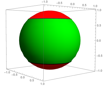
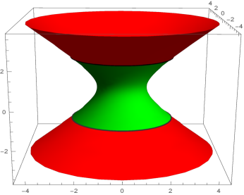
Figure 1: Commutative limit of the Lorentzian fuzzy sphere. Singularities in the metric appear at $\theta=\frac{\pi}{4}$ and $\frac{3\pi}{4}$, and the signature of the metric changes at these latitudes. These latitudes are associated with singularities in the Ricci scalar. The metric tensor has a Euclidean signature for $0<\theta<\frac{\pi}{4}\;\;{\rm and}\;\;\frac{3\pi}{4}<\theta<\pi$ (red regions), and Lorentzian signature for $\frac{\pi}{4}<\theta<\frac{3\pi}{4}$ (green region).

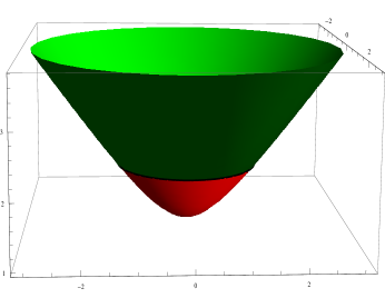
Figure 2: Deformed $AdS_{2}$ solution with $r=1$, $\rho=1.15$. The space-time singularities occur at $\tau=\tau_{\pm}=\pm\tanh^{-1}|\frac{1}{\rho}|$. The green region has Lorentzian signature and the red region has Euclidean signature.

Figure 3: Deformed Euclidean $AdS^{2}$ solution with $r=1$, $\rho=.85$. A space-time singularity occurs at $\tau=\tau_{+}=\tanh^{-1}|\rho|$. The green region has Lorentzian signature and the red region has Euclidean signature.

4 $CP^{1,1}$ and $CP^{0,2}$ solutions

Concerning the generalization to four dimensions, a natural approach would be to examine non-commutative $CP^{2}$.[30]-[36] Actually, if we wish to recover noncompact manifolds in the commutative limit we should consider the indefinite versions of non-commutative $CP^{2}$; non-commutative $CP^{1,1}$ and $CP^{0,2}$. In this section we show that non-commutative $CP^{1,1}$ and $CP^{0,2}$ are solutions to an eight-dimensional matrix model with an indefinite background metric. As with our earlier result, we find no signature change in the absence of a mass term in the action. A mass term will be included in the following section. Here, we begin with some general properties of non-commutative $CP^{1,1}$ and $CP^{0,2}$ in the semi-classical limit, and then construct an eight-dimensional matrix model for which they are solutions.

4.1 Properties

Non-commutative $CP^{p,q}$ was studied in [37]. Here we shall only be interested in its semi-classical limit. $CP^{p,q}$ are hyperboloids $H^{2q,2p+1}$ mod $S^{1}$. They can be defined in terms of $p+q+1$ complex embedding coordinates $z_{i},\;i=1,...,p+q+1$, satisfying the $H^{2q,2p+1}$ constraint

$$\sum_{i=1}^{p+1}z_{i}^{*}z_{i}-\sum_{i=p+2}^{p+q+1}z_{i}^{*}z_{i}=1\;,$$ (4.1)

along with the identification

$$z_{i}\sim e^{i\beta}z_{i}$$ (4.2)

$CP^{p,q}$ can equivalently be defined as the coset space $SU(p+1,q)/U(p,q)$. For the semi-classical limit of non-commutative $CP^{p,q}$ we must also introduce a compatible Poisson structure. For this we take

$$\{z_{i},z^{*}_{j}\}=\left\{\begin{array}[]{ll}-i\delta_{ij}\;,&\mbox{if $\;i,j=1,...,p+1$};\\ \;\;\;i\delta_{ij}\;,&\mbox{if $\;i,j=p+2,...,p+q+1$}\end{array}\right.\;,$$ (4.3)

while all other Poisson brackets amongst $z_{i}$ and $z^{*}_{i}$ vanish. Then one can regard (4.1) as the first class constraint that generates the phase equivalence (4.2).

In specializing to $CP^{1,1}$ and $CP^{0,2}$, it is convenient to introduce the metric $\eta^{C}=$diag$(1,1,-1)$ on the three-dimensional complex space spanned by $z_{i},\;i=1,2,3$. Then writing $z^{i}=(\eta^{C})^{ij}z_{j}$, the constraint (4.1) for $CP^{1,1}$ becomes

$$z^{i}z_{i}^{*}=1\;,$$ (4.4)

while for $CP^{0,2}$ the constraint can be written as

$$\;z^{i}z_{i}^{*}=-1\;$$ (4.5)

For both cases, the Poisson brackets (4.3) become

$$\{z^{i},z^{*}_{j}\}=-i\delta^{i}_{j}\qquad\;\;\{z^{i},z^{j}\}=\{z^{*}_{i},z^{*}_{j}\}=0\;$$ (4.6)

$CP^{1,1}$ and $CP^{0,2}$ can also be described in terms of orbits on $SU(2,1)$. Below we review some properties of the Lie algebra $su(2,1)$. One can write down the defining representation for $su(2,1)$ in terms of traceless $3\times 3$ matrices, $\tilde{\lambda}_{a}$, $a=1,2,...,8$, which are analogous to the Gell-Mann matrices $\lambda_{a}$ spanning $su(3)$. We denote matrix elements by $[\tilde{\lambda}_{a}]^{i}_{\;\,j},\;i,j,..=1,2,3$. Unlike $su(3)$ Gell-Mann matrices, $\tilde{\lambda}_{a}$ are not all hermitean, but instead, satisfy

$$\tilde{\lambda}_{a}\eta^{C}=\eta^{C}\tilde{\lambda}_{a}^{\dagger}$$ (4.7)

They are given in terms of the standard Gell-Mann matrices in Appendix A. The commutation relations for $\tilde{\lambda}_{a}$ are

$$[\tilde{\lambda}_{a},\tilde{\lambda}_{b}]=2i\tilde{f}_{abc}\tilde{\lambda}^{c}\;,$$ (4.8)

where indices $a,b,c...$ are raised and lowered using the Cartan-Killing metric on the eight-dimensional space

$$\eta={\rm diag}(1,1,1,-1,-1,-1,-1,1)\,$$ (4.9)

$\tilde{f}_{abc}$ for $su(2,1)$ are totally antisymmetric. Their values, along with some properties of $su(2,1)$, are given in Appendix A.

$CP^{0,2}$ is the coset space $SU(2,1)/U(2)$. Using the conventions of Appendix A, it is spanned by adjoint orbits in $su(2,1)$ through $\tilde{\lambda}_{8}$, and consists of elements $g\tilde{\lambda}_{8}g^{-1},\;g\in SU(2,1)$. The little group of $\tilde{\lambda}_{8}$ is $U(2)$, which is generated by $\tilde{\lambda}_{1},\tilde{\lambda}_{2},\tilde{\lambda}_{3},\tilde{\lambda}_{8}$. On the other hand, $CP^{1,1}$ is the coset space $SU(2,1)/U(1,1)$. It is corresponds to orbits through

$$\tilde{\Lambda}_{8}=\frac{1}{\sqrt{3}}\pmatrix{-2&&\cr&1&\cr&&1}=-\frac{\sqrt{3}}{2}\tilde{\lambda}_{3}-\frac{1}{2}\tilde{\lambda}_{8}\;,$$ (4.10)

$CP^{1,1}=\{g\tilde{\Lambda}_{8}g^{-1},\;g\in SU(2,1)\}$. The little group of $\tilde{\Lambda}_{8}$ is $U(1,1)$, which is generated by $\tilde{\Lambda}_{8},\tilde{\lambda}_{6},\tilde{\lambda}_{7},\tilde{\Lambda}_{3}=\pmatrix{\;&&\cr&1&\cr&&-1}=-\frac{1}{2}\tilde{\lambda}_{3}+\frac{\sqrt{3}}{2}\tilde{\lambda}_{8}$.

Next, we can construct eight real coordinates $x^{a}$ from $z^{i}$ and $z^{*}_{i}$ using

$$x^{a}=z^{*}_{i}[\tilde{\lambda}^{a}]^{i}_{\;\,j}z^{j}\;,$$ (4.11)

They are invariant under the phase transformation (4.2), and span a four dimensional manifold. Using (A.13), the constraints on the coordinates are

$$x^{a}x_{a}=\frac{4}{3}\qquad\quad\tilde{d}_{abc}x^{b}x^{c}=\pm\frac{2}{3}x_{a}\;,$$ (4.12)

where one takes the upper sign in the second equation for $CP^{1,1}$ and the lower sign for $CP^{0,2}$. $\tilde{d}_{abc}$ is totally symmetric; the values are given in Appendix A. From (4.6), $x_{a}$ satisfy an $su(2,1)$ Poisson bracket algebra

$$\{x_{a},x_{b}\}=2\tilde{f}_{abc}x^{c}$$ (4.13)

4.2 Eight-dimensional matrix model

It is now easy to construct an eight-dimensional ‘IKKT’-type matrix model for which (4.13) is a solution, at least in the commutative limit. As before we only consider the bosonic sector, spanned by eight infinite-dimensional hermitean matrices $X_{a}$, with indices raised and lowered with the indefinite flat metric $\eta_{ab}$. In analogy with the three-dimensional model in (2.1), take the action to consist of a quartic term and a cubic term:

$$S(X)=\frac{1}{{\tt g}^{2}}{\rm Tr}\Bigl{(}-\frac{1}{4}[X_{a},X_{b}][X^{a},X^{b}]+\frac{i}{3}a\,\tilde{f}_{abc}X^{a}[X^{b},X^{c}]\Bigr{)}\;$$ (4.14)

The cubic term appears ad hoc, and we remark that it is actually unnecessary for the purpose of finding solutions when a quadratic term is introduced instead. We consider quadratic terms in section five. On the other hand, the cubic term leads to a richer structure for the space of solutions and it is for that reason we shall consider it.

The equations of motion following from (4.14) are

$$[[X_{a},X_{b}],X^{b}]+ia\,\tilde{f}_{abc}[X^{b},X^{c}]=0$$ (4.15)

They are invariant under unitary ‘gauge’ transformations, $SU(2,1)$ transformations and translations. Assuming that the constant $a$ behaves as in (3.3) in the commutative limit, leads to

$$-\{\{x_{a},x_{b}\},x^{b}\}-\alpha\tilde{f}_{abc}\{x^{b},x^{c}\}=0\;$$ (4.16)

The Poisson brackets (4.13) solve these equations for $\alpha=2$. They describe a $CP^{1,1}$ or $CP^{0,2}$ solution, the choice depending on the sign in the second constraint in (4.12).

For either solution, we can project the eight-dimensional flat metric $\eta$ down to the surface $\bar{z}z=z_{i}^{*}z^{i}=\pm 1\;$, in order to obtain the induced metric. Once again, $i=1,2,3$. Using the Fierz identity (A.13), we get

$$ds^{2}=dx^{a}dx_{a}=4\Bigl{(}(\bar{z}z)(d\bar{z}dz)-|\bar{z}dz|^{2}\Bigr{)}\;,$$ (4.17)

where $\bar{z}dz=z^{*}_{i}dz^{i}$, $d\bar{z}dz=dz_{i}^{*}dz^{i}$ and we have used $d(\bar{z}z)=0$. (4.17) is the Fubini-Study metric written on a noncompact space.

We next examine the induced metric tensor on a local coordinate patch. We choose the local coordinates $(\zeta_{1},\zeta_{2})$, defined by

$$\zeta_{1}=\frac{z^{1}}{z^{3}}\qquad\quad\zeta_{2}=\frac{z^{2}}{z^{3}}\;,\qquad z^{3}\neq 0\;\;,$$ (4.18)

along with their complex conjugates. These coordinates respect the equivalence relation (4.2). In the language of constrained Hamilton formalism, they are first class variables. From their definition it follows that $|\zeta_{1}|^{2}+|\zeta_{2}|^{2}-1=\pm|z^{3}|^{-2}$ and $\bar{z}dz=|z^{3}|^{2}\Bigl{(}\zeta_{1}^{*}d\zeta_{1}+\zeta_{2}^{*}d\zeta_{2}\Bigr{)}\pm d\log z^{3}$, where the upper [lower] sign applies for $CP^{1,1}$ [$CP^{0,2}$]. Substituting into (4.17) gives the induced metric tensor on the coordinate patch

$$\frac{1}{4}ds^{2}\;=\;\frac{1}{2}g_{{}_{\zeta_{u}\zeta_{v}^{*}}}d\zeta_{u}d\zeta_{v}^{*}\;=\;\frac{|d\zeta_{1}|^{2}+|d\zeta_{2}|^{2}}{|\zeta_{1}|^{2}+|\zeta_{2}|^{2}-1}\;-\;\frac{|\zeta_{1}^{*}d\zeta_{1}+\zeta_{2}^{*}d\zeta_{2}|^{2}}{(|\zeta_{1}|^{2}+|\zeta_{2}|^{2}-1)^{2}}\;$$ (4.19)

It has the same form for both $CP^{1,1}$ and $CP^{0,2}$. Because $|\zeta_{1}|^{2}+|\zeta_{2}|^{2}-1<0$ for the latter, $CP^{0,2}$ has Euclidean signature. The Poisson brackets (4.6) can be projected down to the local coordinate patch as well. The result is

$$\{\zeta_{u},\zeta_{v}^{*}\} = \pm i(|\zeta_{1}|^{2}+|\zeta_{2}|^{2}-1)(\zeta_{u}\zeta_{v}^{*}-\delta_{uv})$$ (4.20)

$$\{\zeta_{u},\zeta_{v}\} = \{\zeta_{u}^{*},\zeta_{v}^{*}\}\;=\;0\;,\qquad u,v=1,2$$ (4.22)

Once again, the upper [lower] sign applies for $CP^{1,1}$ [$CP^{0,2}$]. The resulting symplectic two-form is Kähler:

$$\Omega=\mp\frac{i}{2}g_{{}_{\zeta_{u}\zeta_{v}^{*}}}d\zeta_{u}\wedge d\zeta_{v}^{*}$$ (4.23)

Next we re-write the induced metric and symplectic two-form using three Euler-like angles $(\theta,\phi,\psi)$, $0\leq\theta<\pi$, $0\leq\phi<2\pi$, $0\leq\psi<4\pi$, along with one real variable $\tau$, $-\infty<\tau<\infty$. We treat $CP^{1,1}$ and $CP^{0,2}$ separately:

1. $CP^{1,1}\,.\;$ Now write

   $$\zeta_{1}=e^{i(\psi+\phi)/2}\coth\tau\,\cos\frac{\theta}{2}\qquad\qquad\zeta_{2}=e^{i(\psi-\phi)/2}\coth\tau\,\sin\frac{\theta}{2}\;,$$ (4.24)

   which is consistent with the requirement that $|\zeta_{1}|^{2}+|\zeta_{2}|^{2}-1>0$. The induced metic in these coordinates has the Taub-NUT form (which was also true for the $CP^{2}$ solution[12])

   $${ds^{2}} = g_{\tau\tau}\,{d\tau^{2}}+g_{\theta\theta}\,(d\theta^{2}+\sin^{2}\theta d\phi^{2})+g_{\psi\psi}\,(d\psi+\cos\theta d\phi)^{2}\;$$ (4.25)

   We get

   $$g_{\tau\tau}=-4\qquad\quad g_{\theta\theta}=\cosh^{2}\tau\qquad\quad g_{\psi\psi}=-\cosh^{2}\tau\sinh^{2}\tau\;,$$ (4.26)

   with the other nonvanishing components of the induced metric being $g_{\phi\phi}=g_{\psi\psi}\,\cos^{2}\theta+g_{\theta\theta}\,\sin^{2}\theta$ and $g_{\psi\phi}=g_{\psi\psi}\,\cos\theta$. The result indicates that there are two space-like directions and two time-like directions. The symplectic two-form in terms of these coordinates is

   $$\Omega_{{}_{CP^{1,1}}} = -\sinh\tau\cosh\tau\,d\tau\wedge(d\psi+\cos\theta\,d\phi)+\frac{1}{2}\cosh^{2}\tau\sin\theta\,d\theta\wedge d\phi$$ (4.29)

   $$=-\frac{1}{2}\,d\,\Bigl{(}\cosh^{2}\tau\,(d\psi+\cos\theta\,d\phi)\Bigr{)}$$

2. $CP^{0,2}\,.\;$ Here choose

   $$\zeta_{1}=e^{i(\psi+\phi)/2}\tanh\tau\,\cos\frac{\theta}{2}\qquad\qquad\zeta_{2}=e^{i(\psi-\phi)/2}\tanh\tau\,\sin\frac{\theta}{2}\;,$$ (4.30)

   which is consistent with the inequality $|\zeta_{1}|^{2}+|\zeta_{2}|^{2}-1<0$. The resulting induced metric again has the Taub-NUT form (4.25). In contrasting with (4.26), results differ for the $g_{\theta\theta}$ component

   $$g_{\tau\tau}=-4\qquad\quad g_{\theta\theta}=-\sinh^{2}\tau\qquad\quad g_{\psi\psi}=-\cosh^{2}\tau\sinh^{2}\tau\;,$$ (4.31)

   where again $g_{\phi\phi}=g_{\psi\psi}\,\cos^{2}\theta+g_{\theta\theta}\,\sin^{2}\theta$ and $g_{\psi\phi}=g_{\psi\psi}\,\cos\theta$. The induced metric now has a Euclidean signature, and the symplectic two-form is

   $$\Omega_{{}_{CP^{0,2}}} = -\sinh\tau\cosh\tau\,d\tau\wedge(d\psi+\cos\theta\,d\phi)+\frac{1}{2}\sinh^{2}\tau\sin\theta\,d\theta\wedge d\phi$$ (4.34)

   $$=-\frac{1}{2}\,d\,\Bigl{(}\sinh^{2}\tau\,(d\psi+\cos\theta\,d\phi)\Bigr{)}$$

Both metric tensors (4.26) and (4.31) [including the corresponding results for $g_{\phi\phi}$ and $g_{\psi\phi}$] describing $CP^{1,1}$, and $CP^{0,2}$, respectively, are solutions to the sourceless Einstein equations with cosmological constant $\Lambda=\frac{3}{2}$. Obviously, the metric tensors don’t exhibit signature change. In both cases, the sign of the determinant of the metric tensor, det$\,g=g_{\tau\tau}\,g_{\psi\psi}\,(g_{\theta\theta}\,\sin\theta)^{2}$, is positive (away from coordinate singularities).

The above discussion utilized the induced metric tensor. However, the relevant metric in the semi-classical limit for a matrix model solution is not, in general, the induced metric, but rather, it is the metric that appears in the coupling to matter.[15] This is the so-called ‘effective’ metric tensor, which we here denote by $\gamma_{\mu\nu}$. It can be determined from the induced metric $g_{\mu\nu}$ and the symplectric matrix $\Theta^{\mu\nu}$ using

$$\sqrt{|\det\gamma|}\,\gamma^{\mu\nu}=\frac{1}{\sqrt{|\det\Theta|}}\,[\Theta^{T}g\Theta]^{\mu\nu}\,$$ (4.35)

It follows that $|\det\gamma|=|\det g|$, and we can use this identification to determine the effective metric from the induced metric. We review a derivation of (4.35) in Appendix B. In two dimensions, it is known that the effective metric is identical to the induced metric, $\gamma_{\mu\nu}=g_{\mu\nu}$.[38] This is also the case for the $CP^{1,1}$ and $CP^{0,2}$ solutions, as is shown in Appendix B, and so all the previous results that followed from the induced metric also apply for the effective metric. On the other hand, for the solutions of the next section, in addition to finding signature change, we find that the effective metric and induced metric for any particular emergent manifold are in general distinct.

5 Inclusion of a mass term in the $8d$ matrix model

In analogy to section three, we now add a mass term to the matrix model action (4.14),

$$S(X)=\frac{1}{{\tt g}^{2}}{\rm Tr}\Bigl{(}-\frac{1}{4}[X_{a},X_{b}][X^{a},X^{b}]+\frac{i}{3}a\,\tilde{f}_{abc}X^{a}[X^{b},X^{c}]+6\tilde{b}\,X_{a}X^{a}\Bigr{)}\;$$ (5.1)

The matrix equations of motion become

$$[[X_{a},X_{b}],X^{b}]+ia\tilde{f}_{abc}[X^{b},X^{c}]+12\tilde{b}\,X_{a}=0\;,$$ (5.2)

In the semi-classical limit $\hbar\rightarrow 0$, we take $a\rightarrow\hbar\alpha$, along with $\tilde{b}\rightarrow\hbar^{2}\tilde{\beta}$. Then (5.2) goes to

$$-\{\{x_{a},x_{b}\},x^{b}\}-\alpha\tilde{f}_{abc}\{x^{b},x^{c}\}+12\tilde{\beta}x_{a}=0\;,$$ (5.3)

These equations are solved by (4.13) for

$$\alpha=2(1+\tilde{\beta})$$ (5.4)

Thus $CP^{1,1}$ and $CP^{0,2}$ are solutions to the massive matrix model. In the limit where the mass term vanishes, $\tilde{\beta}=0$ and $\alpha=2$, we recover the solutions of the previous section. $CP^{1,1}$ and $CP^{0,2}$ solutions also persist in the absence of the cubic term in the matrix model action (5.1). For this we need $\alpha=0$ and $\tilde{\beta}=-1$. The mass term allows for other solutions which have no $\beta\rightarrow 0$ limit. Among these solutions are the deformations of $CP^{1,1}$ and $CP^{0,2}$, as well as deformations of $CP^{2}$, which we discuss in the following subsections.

5.1 Deformations of $CP^{1,1}$ and $CP^{0,2}$

For deformations of $CP^{1,1}$ and $CP^{0,2}$ we modify the ansatz (4.11) to

$$x_{1-3} = \mu\,z^{*}_{i}[\tilde{\lambda}_{1-3}]^{i}_{\;\,j}z^{j}$$ (5.5)

$$x_{4-7} = \;\;z^{*}_{i}[\tilde{\lambda}_{4-7}]^{i}_{\;\,j}z^{j}$$ (5.7)

$$x_{8} = \nu\,z^{*}_{i}[\tilde{\lambda}_{8}]^{i}_{\;\,j}z^{j}\;,$$ (5.9)

where $\mu$ and $\nu$ are deformation parameters, which we shall restrict to be real. This is a solution to the equations (5.3) provided that the following relations hold amongst the parameters:

$$(2\mu-\alpha)\Bigl{(}\mu^{2}+\frac{1}{2}\Bigr{)}+3\mu\tilde{\beta} = 0$$ (5.10)

$$\mu^{2}+\nu^{2}+2-\alpha(\mu+\nu)+4\tilde{\beta} = 0$$ (5.12)

$$2\nu-\alpha+2\nu\tilde{\beta} = 0$$ (5.14)

These relations reduce to (5.4) when $\mu=\nu=1$, and so we recover undeformed $CP^{1,1}$ and $CP^{0,2}$ in this limit. For generic values of the parameters, there are nontrivial solutions to these algebraic relations, which can be expressed as functions of the mass parameter $\tilde{\beta}$. For a particular choice of signs:

$$\alpha={2\mu}\,\frac{\tilde{\beta}^{2}-\tilde{\beta}-1-\gamma[\tilde{\beta}]}{2\tilde{\beta}+1}\qquad\quad\mu={\sqrt{\frac{\tilde{\beta}^{3}-4\tilde{\beta}^{2}-6\tilde{\beta}+\tilde{\beta}\gamma[\tilde{\beta}]-2}{2(\tilde{\beta}^{2}+4\tilde{\beta}+2)}}}\qquad\quad\nu=\frac{\alpha}{2(1+\tilde{\beta})}\;,$$ (5.15)

where

$$\gamma[\tilde{\beta}]=\sqrt{\tilde{\beta}^{4}-12\tilde{\beta}^{3}-22\tilde{\beta}^{2}-12\tilde{\beta}-2}$$ (5.16)

Upon requiring $\gamma[\tilde{\beta}]$ to be real, we obtain three disconnected intervals $i-iii)$ in $\tilde{\beta}$:

$$i)\;\;\qquad\qquad\qquad\qquad\qquad\qquad\qquad\qquad\qquad\quad \tilde{\beta} \leq\;\,\frac{1}{2}\left(6-3\sqrt{6}-\sqrt{98+40\sqrt{6}}\right)\approx-0.746$$ (5.17)

$$ii)\quad\frac{1}{2}\left(6-3\sqrt{6}+\sqrt{98+40\sqrt{6}}\right)\approx-0.603\;\,\leq \tilde{\beta} \leq\,\;\frac{1}{2}\left(6+3\sqrt{6}-\sqrt{98+40\sqrt{6}}\right)\approx-0.325$$ (5.19)

$$iii)\quad\frac{1}{2}\left(6+3\sqrt{6}+\sqrt{98+40\sqrt{6}}\right)\;\approx\;\,13.67\;\,\leq \tilde{\beta}$$ (5.21)

We further restrict $\mu$ to be real. (Reality of $\alpha$ and $\nu$ then follows.) For solution (5.15), this reduces the acceptable regions in $\tilde{\beta}$ to

$$i^{\prime})\;-3.414\lesssim\tilde{\beta}\lesssim-0.746\;,\qquad\quad\;ii^{\prime})\;\;-0.603\,\lesssim\,\tilde{\beta}\,\lesssim\,-0.586\;,\qquad\quad\;iii)\;13.67\,\lesssim\,\tilde{\beta}$$ (5.22)

When $\tilde{\beta}=-.6\,$, we recover the undeformed case $\mu=\nu=1$ (along with $\alpha=.8)\,$. Therefore, matrix solutions in the range $\;ii^{\prime})$ can be regarded as continuous deformations of the undeformed solutions, while those in the ranges $\;i^{\prime})$ and $\;iii)$ cannot be continuously connected to the undeformed solutions.

In addition to the family of solutions given in (5.15) and (5.16), the equations (5.14) have the simple solution:

$$\alpha=\nu=0\qquad\quad\tilde{\beta}=-\frac{3}{5}\qquad\quad\mu^{2}=\frac{2}{5}$$ (5.23)

It is a solution for the case where the cubic term in the matrix model action (5.1) is absent. From (5.9), $\nu=0$ implies that the projection of the solution along the $8^{\rm th}$-direction vanishes, $x_{8}=0$. This solution is not contained in (5.15) and (5.16).

The ansatz (5.9) for $\mu$ and $\nu$ not both equal to one, leads to two types of solutions:

1. Deformed $CP^{1,1}$, where the complex coordinates $z^{i}$ satisfy the constraint (4.4), and

2. Deformed $CP^{0,2}$, where the complex coordinates $z^{i}$ satisfy (4.5).

We next compute the induced metric for these two types of solutions.

5.1.1 Induced metric

The induced metric is again computed by projecting the eight-dimensional flat metric (4.9) onto the surface. From the ansatz (5.9) we get

$$ds^{2}=dx^{a}dx_{a} = 4(|z_{1}|^{2}+|z_{2}|^{2}-|z_{3}|^{2})(|dz_{1}|^{2}+|dz_{2}|^{2}-|dz_{3}|^{2})-4|z^{*}_{1}dz_{1}+z^{*}_{2}dz_{2}-z^{*}_{3}dz_{3}|^{2}$$ (5.24)

$$+ 4(\mu^{2}-1)(|z_{1}|^{2}+|z_{2}|^{2})(|dz_{1}|^{2}+|dz_{2}|^{2})+(\mu^{2}-1)(z^{*}_{1}dz_{1}+z^{*}_{2}dz_{2}-z_{1}dz^{*}_{1}-z_{2}dz^{*}_{2})^{2}$$ (5.26)

$$+ \frac{1}{3}(\nu^{2}-1)(z^{*}_{1}dz_{1}+z^{*}_{2}dz_{2}+2z^{*}_{3}dz_{3}+z_{1}dz^{*}_{1}+z_{2}dz^{*}_{2}+2z_{3}dz^{*}_{3})^{2}$$ (5.28)

We have not yet specialized to the two cases 1. and 2.

The result (LABEL:dfrmmtrc) can be rewritten in terms of the local coordinates $(\zeta_{1},\zeta_{2})$, defined in (4.18), according to

$$ds^{2} = 4|z_{3}|^{2}\Bigl{(}-|z_{3}|^{2}|\Xi|^{2}\pm(|d\zeta_{1}|^{2}+|d\zeta_{2}|^{2})\Bigr{)}$$ (5.30)

$$+ 4(\mu^{2}-1)(|z_{3}|^{2}\pm 1)\Bigl{(}(1\pm|z_{3}|^{-2})|dz_{3}|^{2}+|z_{3}|^{2}(|d\zeta_{1}|^{2}+|d\zeta_{2}|^{2})+\Xi\,z_{3}dz_{3}^{*}+\Xi^{*}z_{3}^{*}dz_{3}\,\Bigr{)}$$ (5.32)

$$+ (\mu^{2}-1)\Bigl{(}|z_{3}|^{2}(\Xi-\Xi^{*})+(1\pm|z_{3}|^{-2})(z^{*}_{3}dz_{3}-z_{3}dz_{3}^{*})\Bigr{)}^{2}\;+\;(\nu^{2}-1)\Bigl{(}d|z_{3}|^{2}\Bigr{)}^{2}\;,$$ (5.34)

where $\Xi=\zeta_{1}^{*}d\zeta_{1}+\zeta_{2}^{*}d\zeta_{2}$ and we have used $|\zeta_{1}|^{2}+|\zeta_{2}|^{2}=1\pm|z_{3}|^{-2}$. The upper [lower] sign applies for deformed $CP^{1,1}$ [$CP^{0,2}$]. The expression (LABEL:dfmtczta) simplifies after making the gauge choice that $z_{3}$ is real, which we shall do below.

The signature of the induced metric becomes more evident after expressing it in terms of the three Euler-like angles $\theta,\phi,\psi$, along with parameter $\tau$ spanning $R_{+}$, as we did in section four for the undeformed metrics. For this we now specialize to the two cases: 1. deformed $CP^{1,1}$ and 2. deformed $CP^{0,2}$ .

1. Deformed $CP^{1,1}\,.\;$

   For this case we can apply coordinate transformation (4.24). Upon making the phase choice $z_{3}=\sinh\tau$, (LABEL:dfmtczta) can be written in the Taub-NUT form (4.25), where the metric components are now

   $$g_{\tau\tau} = 4\Bigl{(}(\mu^{2}+\nu^{2}-2)\cosh^{2}\tau\,{\sinh^{2}\tau}-1\Bigr{)}$$ (5.36)

   $$g_{\theta\theta} = \cosh^{2}\tau\,(\mu^{2}\cosh^{2}\tau-\sinh^{2}\tau)$$ (5.38)

   $$g_{\psi\psi} = -\cosh^{2}\tau\sinh^{2}\tau$$ (5.40)

   The remaining nonvanishing components of the induced metric are again obtained from $g_{\phi\phi}=g_{\psi\psi}\,\cos^{2}\theta+g_{\theta\theta}\,\sin^{2}\theta$ and $g_{\psi\phi}=g_{\psi\psi}\,\cos\theta$. The undeformed $CP^{1,1}$ induced metric tensor in (4.26) is recovered from (5.40) upon setting $\mu=\nu=1$. This limit thus corresponds to there being two space-like directions and two time-like directions, with sign$(g_{\tau\tau},g_{\theta\theta})=(-,+)$ and det$\;g>0$ (away from coordinate singularities). The same two space-like directions and two time-like directions appear in the limit $|\tau|\rightarrow 0$. Signature change can occur when we go away from either of these two limits, as we describe below:

   For the solutions given by (5.15) and (5.16), given some value of $\tilde{\beta}$ $(\neq-1,-.6)$ in the regions $i^{\prime}$, $ii^{\prime})$ and $iii)$, the sign of either $g_{\tau\tau}$ or $g_{\theta\theta}$ changes at some value of $|\tau|$. We plot the values of $|\tau|$ versus $\tilde{\beta}$ for which this occurs in figure 4. $g_{\tau\tau}$ changes sign when $(\mu^{2}+\nu^{2}-2)\sinh^{2}\tau\cosh^{2}\tau=1\,$ (indicated by the red curves in figure 4). $g_{\theta\theta}$ changes sign when $\tanh^{2}\tau=\mu^{2}$ (indicated by the green curves in figure 4). Above the red curves, sign $(g_{\tau\tau},g_{\theta\theta})=(+,+)$ and det$\;g<0$ and so the induced metric has Lorentzian signature in this region. In this case, the time-like direction corresponds to $d\psi+\cos\theta d\phi$. It corresponds to a space-time with closed time-like curves. Above the green curves, sign$(g_{\tau\tau},g_{\theta\theta})=(-,-)$, while det$\;g>0$. In this case, the induced metric space has a Euclidean signature.

   For the solution (5.23), a sign change in $g_{\theta\theta}$ occurs at $\tanh^{2}\tau=\frac{2}{5}$, and the induced metric has a Euclidean signature for $\tanh^{2}\tau>\frac{2}{5}$.

   

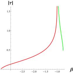
   (a) region $i^{\prime})$

   

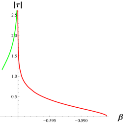
   (b) region $\;ii^{\prime})$

   

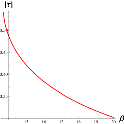
   (c) region $iii)$

   Figure 4: Signature changes in the induced metric $g_{\mu\nu}$ and effective metric $\gamma_{\mu\nu}$ for deformed $CP^{1,1}$ are given in plots of $|\tau|$ versus $\tilde{\beta}$ for in the three disconnected regions: $i^{\prime})\;-3.414\lesssim\tilde{\beta}\lesssim-0.746$ (subfigure a), $\;ii^{\prime})\;\;-0.603\,\lesssim\,\tilde{\beta}\,\lesssim\,-0.586\;$ (subfigure b) and $iii)\;13.67\;\lesssim\,\tilde{\beta}$ (subfigure c). A sign change in $g_{\theta\theta}$ or $\gamma_{\theta\theta}$ is indicated by the green curves. Sign change in $g_{\tau\tau}$ or $\gamma_{\psi\psi}$ is indicated by the red curves.

2. Deformed $CP^{0,2}\,.\;$

   Here we apply the coordinate transformation (4.30) to (LABEL:dfmtczta), along with the phase choice $z_{3}=\cosh\tau$. The induced invariant interval again takes the Taub-NUT form (4.25), with the matrix elements now being

   $$g_{\tau\tau} = 4\Bigl{(}(\mu^{2}+\nu^{2}-2)\cosh^{2}\tau\,{\sinh^{2}\tau}-1\Bigr{)}$$ (5.41)

   $$g_{\theta\theta} = \sinh^{2}\tau\,\Bigl{(}\mu^{2}\sinh^{2}\tau-\cosh^{2}\tau\Bigr{)}$$ (5.43)

   $$g_{\psi\psi} = -\cosh^{2}\tau\sinh^{2}\tau\;,$$ (5.45)

   and $g_{\phi\phi}=g_{\psi\psi}\,\cos^{2}\theta+g_{\theta\theta}\,\sin^{2}\theta$ and $g_{\psi\phi}=g_{\psi\psi}\,\cos\theta$. Only the results for $g_{\theta\theta}$ differ in expressions (5.40) and (5.45). The latter reduce to that of undeformed $CP^{0,2}$, (4.31), when $\mu=\nu=1$. For that limit, as well as for $|\tau|\rightarrow 0$, sign$(g_{\tau\tau},g_{\theta\theta})=(-,-)$ and det$\;g>0$ (away from coordinate singularities). In this case, the induced metric has a Euclidean signature. As with deformed $CP^{1,1}$, signature change can occur when we go away from these limits, as we describe below:

   For the solutions given by (5.15) and (5.16), we find that for any fixed value of $\tilde{\beta}$ in the regions $i^{\prime})$, $\;ii^{\prime})$ and $iii)$, either a sign change occurs for both $g_{\tau\tau}$ and $g_{\theta\theta}$, or there is no signature change. We plot the signature changes for deformed $CP^{0,2}$ in figure 5. $g_{\theta\theta}$ changes sign when $\coth^{2}\tau=\mu^{2}$ (indicated by the green curves in figure 5). $g_{\tau\tau}$ changes sign when $(\mu^{2}+\nu^{2}-2)\sinh^{2}\tau\cosh^{2}\tau=1\,$ (indicated by the red curves in figure 5). We find that there are no sign changes in the induced metric for $-1<\tilde{\beta}\lesssim-0.746$ and $-0.603\,\lesssim\,\tilde{\beta}\,\leq-.6$. So for these sub-regions, the signature of the induced metric remains Euclidean for all $\tau$. For the complementary sub-regions, a sign change occurs in $g_{\tau\tau}$, say at $|\tau|=|\tau_{1}|$, and $g_{\theta\theta}$, at a later $|\tau|$, say $|\tau_{2}|$, i.e., $|\tau_{2}|>|\tau_{1}|$. For $|\tau|>|\tau_{2}|$, sign$(g_{\tau\tau},g_{\theta\theta})=(+,+)$, and so the induced metric has a Lorentzian signature in this case. The time-like direction corresponds to $d\psi+\cos\theta d\phi$, once again corresponding to a space-time with closed time-like curves. For the intermediate interval in $|\tau|$ where $|\tau_{1}|<|\tau|<|\tau_{2}|$, we get sign$(g_{\tau\tau},g_{\theta\theta})=(+,-)$. In this case, the induced metric has a Lorentzian signature, with $\tau$ defining the time-like direction. Any $\tau-$slice is topologically a three-sphere, since from (4.30),

   $$|\zeta_{1}|^{2}+|\zeta_{2}|^{2}=\tanh^{2}\tau$$ (5.46)

   Restricting to positive $\tau$, the interval $\tau_{1}<\tau<\tau_{2}$ has an initial singularity at $\tau_{1}$, and final singularity at $\tau_{2}$. Therefore, although not very realistic, it describes a closed space-time cosmology.

   No signature change in the induced metric results from the solution (5.23).

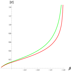
(a) region $i^{\prime})$

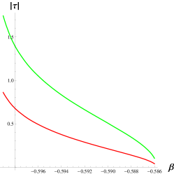
(b) region $\;ii^{\prime})$

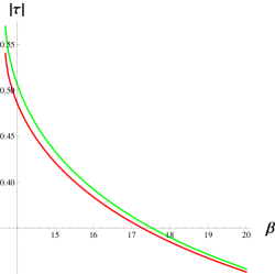
(c) region $iii)$

Figure 5: Signature changes in the induced metric $g_{\mu\nu}$ and effective metric $\gamma_{\mu\nu}$ for deformed $CP^{0,2}$ are given in plots of $|\tau|$ versus $\tilde{\beta}$ for in the three disconnected regions: $i^{\prime})\;-3.414\lesssim\tilde{\beta}\lesssim-0.746$ (subfigure a), $\;ii^{\prime})\;\;-0.603\,\lesssim\,\tilde{\beta}\,\lesssim\,-0.586\;$ (subfigure b) and $iii)\;13.67\;\lesssim\,\tilde{\beta}$ (subfigure c). A sign change in $g_{\theta\theta}$ or $\gamma_{\theta\theta}$ is indicated by the green curves. A sign change in $g_{\tau\tau}$ or $\gamma_{\psi\psi}$ is indicated by the red curves. No sign changes occur in either the induced metric or effective metric for $-1<\tilde{\beta}\lesssim-0.746$ and $-0.603\,\lesssim\,\tilde{\beta}\,\leq-.6\,$.

We remark that while the induced metrics for the two solutions 1. and 2. are modified from their undeformed counterparts, their Poisson brackets, and corresponding symplectic two-forms, are unchanged. That is, for deformed $CP^{1,1}$ the symplectic two-form is (4.29) and for deformed $CP^{0,2}$ symplectic two-form is (4.34). This is relevant for the computation of the effective metric, which we do in the following subsection.

5.1.2 Effective metric

In section four we found that the induced metric $g_{\mu\nu}$ and effective metric $\gamma_{\mu\nu}$ for undeformed $CP^{1,1}$ and $CP^{0,2}$ are identical. The same result does not hold for the corresponding deformed solutions, as we show below. Furthermore, more realistic cosmologies follow from the effective metric of the deformed $CP^{1,1}$ and $CP^{0,2}$ solutions.

1. Deformed $CP^{1,1}\,.\;$ To compute the effective metric we need the symplectic matrix, as well as the induced metric. For the deformed, as well as undeformed, $CP^{1,1}$ solutions, the nonvanishing components of the inverse symplectic matrix are given in (B.8), while the induced metric for deformed $CP^{1,1}$ is given by (5.40). In addition, $|\det\Theta|$ is given in (B.9), while $\;|\det\gamma|$ gets deformed, such that

   $$|\det\gamma||\det\Theta|=4|g_{\tau\tau}|\,(\mu^{2}\cosh^{2}\tau-\sinh^{2}\tau)^{2}\;,$$ (5.47)

   with $g_{\tau\tau}$ given in (5.40). As a result, the nonvanishing components of the effective metric tensor are given by

   $$\frac{\gamma_{\tau\tau}}{\sqrt{|\det\gamma||\det\Theta|}} = -1$$ (5.48)

   $$\frac{\gamma_{\theta\theta}}{\sqrt{|\det\gamma||\det\Theta|}} = \frac{1}{4(\mu^{2}-\tanh^{2}\tau)}$$ (5.50)

   $$\frac{\gamma_{\psi\psi}}{\sqrt{|\det\gamma||\det\Theta|}} = -\frac{1}{4({\rm sech}^{2}\tau\,{\rm csch}^{2}\tau+2-\mu^{2}-\nu^{2})}\;,$$ (5.52)

   in addition to $\gamma_{\phi\phi}=\gamma_{\psi\psi}\,\cos^{2}\theta+\gamma_{\theta\theta}\,\sin^{2}\theta$ and $\gamma_{\psi\phi}=\gamma_{\psi\psi}\,\cos\theta$. The results again agree with the undeformed induced metric (4.26) in the $\mu=\nu=1$ limit. This limit has two space-like directions and two time-like directions, with sign$(\gamma_{\psi\psi},\gamma_{\theta\theta})=(-,+)$ and det$\;\gamma>0$ (away from coordinate singularities). Signature changes occur in the effective metric for the same values of the parameters at which the signature changes occur for the induced metric.

   For the solutions given by (5.15) and (5.16), signature changes are again given in figure 4. A sign change in $\gamma_{\theta\theta}$ [as with $g_{\theta\theta}$] appears when $\tanh^{2}\tau=\mu^{2}$ (indicated by the green curves in figure 4). The effective metric has a Euclidean signature above the green curves. A sign change in $\gamma_{\psi\psi}$ [as with $g_{\tau\tau}$] appears when $(\mu^{2}+\nu^{2}-2)\sinh^{2}\tau\cosh^{2}\tau=1\,$ (indicated by the red curves in figure 4). Above the red curves, the signature of the effective metric is Lorentzian, det$\;\gamma<0$, and $\tau$ is the time-like direction. A $\tau-$slice again defines a three-sphere, since from (4.24),

   $$|\zeta_{1}|^{2}+|\zeta_{2}|^{2}=\coth^{2}\tau$$ (5.53)

   Restricting to positive $\tau$, this region with Lorentzian signature has an initial singularity, and therefore, and it describes an open space-time. We shall see in the next subsection that it corresponds to an expanding cosmology.

   For the solution (5.23), a sign change in $\gamma_{\theta\theta}$ occurs at $\tanh^{2}\tau=\frac{2}{5}$, and the effective metric has a Euclidean signature for $\tanh^{2}\tau>\frac{2}{5}$. There are no regions with Lorentzian signature in this case.

2. Deformed $CP^{0,2}\,.\;$ We repeat the above calculation to get the effective metric $\gamma_{\mu\nu}$ for deformed $CP^{0,2}\,.$ The inverse symplectic matrix is the same as for undeformed $CP^{0,2}\,,$ with nonvanishing components (B.11). The induced metric for deformed $CP^{0,2}$ is given in (5.45). Using the result for $|\det\Theta|$ in (B.12), we now get

   $$|\det\gamma||\det\Theta|=4|g_{\tau\tau}|\,(\mu^{2}\sinh^{2}\tau-\cosh^{2}\tau)^{2}\;,$$ (5.54)

   with $g_{\tau\tau}$ given in (5.45). Now the nonvanishing components of the effective metric tensor are found to be

   $$\frac{\gamma_{\tau\tau}}{\sqrt{|\det\gamma||\det\Theta|}} = -1$$ (5.55)

   $$\frac{\gamma_{\theta\theta}}{\sqrt{|\det\gamma||\det\Theta|}} = \frac{1}{4(\mu^{2}-{\rm coth}^{2}\tau)}$$ (5.57)

   $$\frac{\gamma_{\psi\psi}}{\sqrt{|\det\gamma||\det\Theta|}} = \frac{1}{4(\mu^{2}+\nu^{2}-2-4\,{\rm csch}^{2}2\tau)}\;,$$ (5.59)

   again with $\gamma_{\phi\phi}=\gamma_{\psi\psi}\,\cos^{2}\theta+\gamma_{\theta\theta}\,\sin^{2}\theta$ and $\gamma_{\psi\phi}=\gamma_{\psi\psi}\,\cos\theta$. The results reduce to the undeformed induced metric (4.31) in the limit $\mu=\nu=1$, describing a space with Euclidean signature.

   For the solution given by (5.15) and (5.16), signature changes in the effective metric occur at the same values of the parameters as the signature changes for the induced metric, which are indicated in figure 5. $\gamma_{\theta\theta}$ [like $g_{\theta\theta}$] changes sign when ${\rm coth}^{2}\tau=\mu^{2}$ (indicated by the green curves in figure 5). $\gamma_{\psi\psi}$ [like $g_{\tau\tau}$] changes sign when $(\mu^{2}+\nu^{2}-2)\sinh^{2}\tau\cosh^{2}\tau=1\,$ (indicated by the red curves in figure 5). As seen in the figure, given any fixed value of $\tilde{\beta}$ in the regions $i^{\prime})\;,\;ii^{\prime})$ and $iii)$, either a sign change occurs in both $\gamma_{\psi\psi}$ and $\gamma_{\theta\theta}$, or there is no signature change. No sign changes in the effective metric for $-1<\tilde{\beta}\lesssim-0.746$ and $-0.603\,\lesssim\,\tilde{\beta}\,\leq-.6$. So for these sub-regions the signature of the induced metric remains Euclidean. For the complementary regions, a sign change occurs in $\gamma_{\psi\psi}$ at $|\tau|=|\tau_{1}|$ and $\gamma_{\theta\theta}$ at and $|\tau|=|\tau_{2}|$, with $|\tau_{2}|>|\tau_{1}|$. In the intermediate region $|\tau_{1}|<|\tau|<|\tau_{2}|$, sign$(\gamma_{\psi\psi},\gamma_{\theta\theta})=(+,-)$. Here the effective metric has a Lorentzian signature, but unlike what happens with the induced metric, $d\psi+\cos\theta d\phi$ is associated with the time-like direction, yielding closed time-like curves. For $|\tau|>|\tau_{2}|$, i.e., above the green curves, sign$(\gamma_{\psi\psi},\gamma_{\theta\theta})=(+,+)$, and so the effective metric picks up a Lorentzian signature, with $\tau$ being the time-like direction. From (5.46), a $\tau-$slice is a 3-sphere. Restricting to positive $\tau$, this region with Lorentzian signature has an initial singularity, and so describes a open space-time cosmology, which we next show, is expanding.

   No signature change in the effective metric results from the solution (5.23).

5.1.3 Expansion

From the deformed $CP^{1,1}$ and $CP^{0,2}$ solutions we found regions in parameter space where the effective metric has a Lorentzian signature, and possessed an initial singularity. Any time ($\tau$) - slice is a three-sphere, or more precisely, a Berger sphere. These examples correspond to space-time cosmologies with a big bang. To show that they are expanding we introduce a spatial scale $a(|\tau|)$. We define it as the cubed root of the three-volume at any $\tau-$slice

$$a(|\tau|)^{3}=\int_{S^{3}}\sqrt{|\det\gamma^{(3)}|}\,d\theta d\phi d\psi\;,$$ (5.60)

where $\gamma^{(3)}$ denotes the effective metric on the $\tau-$slice. From the form of the metric tesnor, det$\,\gamma^{(3)}=\gamma_{\psi\psi}\,(\gamma_{\theta\theta}\,\sin\theta)^{2}$, and since $\gamma_{\psi\psi}$ and $\gamma_{\theta\theta}$ only depend on $\tau$. Then

$$a(|\tau|)^{3}=(4\pi)^{2}\sqrt{|\gamma_{\psi\psi}|}\,|\gamma_{\theta\theta}|$$ (5.61)

We wish to determine how the spatial scale evolves with respect to the proper time $t$ in the co-moving frame

$$t(\tau) = \int_{\tau_{0}}^{\tau}\sqrt{-\gamma_{\tau\tau}(\tau^{\prime})}\;d\tau^{\prime}\,$$ (5.62)

$$= \,\int_{\tau_{0}}^{\tau}|\det\gamma(\tau^{\prime})|^{\frac{1}{4}}|\det\Theta(\tau^{\prime})|^{\frac{1}{4}}\,d\tau^{\prime}$$ (5.64)

The lower integration limit $\tau_{0}$ corresponds to the value of $\tau$ at the big bang, i.e., the signature change.

We next compute and plot $a(|\tau|)$ versus $t(\tau)$ for the two cases, deformed $CP^{1,1}$ and deformed $CP^{0,2}$, in the regions of Lorentzian signature:

1. Deformed $CP^{1,1}$. For the spatial volume, we get

   $$a(|\tau|)^{3}={(4\pi)^{2}\,\cosh^{3}\tau|\sinh\tau|\,|\mu^{2}\cosh^{2}\tau-\sinh^{2}\tau|^{\frac{1}{2}}\,\Big{|}(\mu^{2}+\nu^{2}-2)\cosh^{2}\tau\,{\sinh^{2}\tau}-1\Big{|}^{\frac{1}{4}}}\;,$$ (5.65)

   after substituting (5.40) and (5.47) into (5.61). For the proper time $t(|\tau|)$ in the co-moving frame we get

   $$t(\tau)\,={2}\,\int_{\tau_{0}}^{\tau}\,{|\mu^{2}\cosh^{2}\tau^{\prime}-\sinh^{2}\tau^{\prime}|}^{\frac{1}{2}}\;\Big{|}(\mu^{2}+\nu^{2}-2)\cosh^{2}\tau^{\prime}\,{\sinh^{2}\tau^{\prime}}-1\Big{|}^{\frac{1}{4}}d\tau^{\prime}\;,$$ (5.66)

   and $\tau_{0}$ is associated with the signature change, given by $\;{\sinh^{2}2\tau_{0}}=\frac{4}{(\mu^{2}+\nu^{2}-2)}$. It corresponds to value of $\tau$ at the initial singularity, where from (5.65), the spatial scale vanishes. In figure 6(a) we plot $a(|\tau|)$ versus $t(\tau)$ for regions of deformed $CP^{1,1}$ where the effective metric has Lorentzian signature, using three values of $\tilde{\beta}$. It shows a very rapid expansion near the origin. For $\tau$ close to $\tau_{0}$, (5.65) and (5.66) give $a\sim(\tau-\tau_{0})^{\frac{1}{12}}$ and $t\sim(\tau-\tau_{0})^{\frac{5}{4}}$. Hence, $a\sim t^{\frac{1}{15}}$. For large $\tau$, $a$ is linear in $t$. The same large distance behavior was found for solutions in [13].

2. For deformed $CP^{0,2}$, (5.61) gives

   $$a(|\tau|)^{3}={(4\pi)^{2}\,|\sinh\tau|^{3}\cosh\tau|\mu^{2}\sinh^{2}\tau-\cosh^{2}\tau|^{\frac{1}{2}}\Big{|}(\mu^{2}+\nu^{2}-2)\cosh^{2}\tau\,{\sinh^{2}\tau}-1\Big{|}^{\frac{1}{4}}}\;,$$ (5.67)

   after using (5.45) and from (5.54). (5.64) gives

   $$t(\tau)\,=2\,\int_{\tau_{0}}^{\tau}{|\mu^{2}\sinh^{2}\tau^{\prime}-\cosh^{2}\tau^{\prime}|}^{\frac{1}{2}}\;\Big{|}(\mu^{2}+\nu^{2}-2)\cosh^{2}\tau^{\prime}\,{\sinh^{2}\tau^{\prime}}-1\Big{|}^{\frac{1}{4}}\,d\tau^{\prime}$$ (5.68)

   Again, the initial value $\tau_{0}$ for $\tau$ is associated with a signature change, now satisfying $\coth^{2}\tau_{0}=\mu^{2}$. It corresponds to a big-bang singularity, and from (5.67), $a(|\tau_{0}|)=0$. In figure 6(b) we plot $a(|\tau|)$ versus $t(\tau)$ for regions of deformed $CP^{0,2}$ where the effective metric has Lorentzian signature, using three values of $\tilde{\beta}$. It too shows a rapid expansion near the origin. For $\tau$ close to $\tau_{0}$, (5.67) and (5.68) give $a\sim(\tau-\tau_{0})^{\frac{1}{6}}$ and $t\sim(\tau-\tau_{0})^{\frac{3}{2}}$. Hence, $a\sim t^{\frac{1}{9}}$. As with the case of deformed $CP^{1,1}$ and [13], $a\sim t$ for large $\tau$.

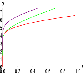
(a) deformed $CP^{1,1}$

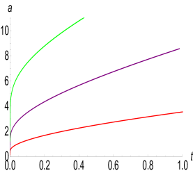
(b) deformed $CP^{0,2}$

Figure 6: $a(|\tau|)$ versus $t(\tau)$ for regions of deformed $CP^{1,1}$ (subfigure a) and deformed $CP^{0,2}$ (subfigure b) where the effective metric has Lorentzian signature (and $\tau$ is the time-like direction) for $\tilde{\beta}=-3$ (red curve), $-.595$ (green curve) and $14$ (purple curve).

5.2 Deformed $CP^{2}$

We now look for solutions to the previous eight-dimensional matrix model which are deformations of non-commutative $CP^{2}$. $CP^{2}$ is a solution to an eight-dimensional matrix model in a Euclidean background. In [12], such solutions were found when the background metric was changed to diag($+,+,+,+,+,+,+,-)$. Here we show that deformations of non-commutative $CP^{2}$ solve the matrix model with the indefinite metric (4.9), and that they may be associated with multiple signature changes.

We once again assume that the three complex coordinates $z_{i}$ satisfy the constraint (4.4), but now that the indices are raised and lowered with the three-dimensional Euclidean metric. The Poisson brackets that arise from the commutative limit of fuzzy $CP^{2}$ are (4.6) [now, assuming the Euclidean metric] [12]. We replace the $su(2,1)$ Gell-Mann matrices $\tilde{\lambda}_{a}$ in (5.9) by $su(3)$ Gell-Mann matrices $\lambda_{a}$, i.e.,

$$x_{1-3} = \mu\,z^{*}_{i}[\lambda_{1-3}]^{i}_{\;\,j}z^{j}$$ (5.69)

$$x_{4-7} = \;\;z^{*}_{i}[\lambda_{4-7}]^{i}_{\;\,j}z^{j}$$ (5.71)

$$x_{8} = \nu\,z^{*}_{i}[\lambda_{8}]^{i}_{\;\,j}z^{j}\;,$$ (5.73)

Now substitute this ansatz into the equations of motion (5.3) to get the following conditions on the parameters

$$(2\mu-\alpha)\Bigl{(}\mu^{2}-\frac{1}{2}\Bigr{)}+3\mu\tilde{\beta} = 0$$ (5.74)

$$\mu^{2}+\nu^{2}-2-\alpha(\mu+\nu)+4\tilde{\beta} = 0$$ (5.76)

$$2\nu(\tilde{\beta}-1)+\alpha = 0\;,$$ (5.78)

which differs from (5.14) in various signs. We can obtain (5.78) by making the replacement $(\alpha,\tilde{\beta},\mu,\nu)\rightarrow(i\alpha,-\tilde{\beta},i\mu,i\nu)$ in (5.14). To obtain a solution to (5.78), we can then make the same replacement in the solution (5.15). The result is

$$\alpha={2\mu}\,\frac{\tilde{\beta}^{2}+\tilde{\beta}-1-\gamma[-\tilde{\beta}]}{-2\tilde{\beta}+1}\qquad\quad\mu={\sqrt{\frac{\tilde{\beta}^{3}+4\tilde{\beta}^{2}-6\tilde{\beta}+\tilde{\beta}\gamma[-\tilde{\beta}]+2}{2(\tilde{\beta}^{2}-4\tilde{\beta}+2)}}}\qquad\quad\nu=\frac{\alpha}{2(1-\tilde{\beta})}\;,$$ (5.79)

where $\gamma[\tilde{\beta}]$ was defined in (5.16). The parameters $\mu$, $\nu$, and $\alpha$ (and necessarily, $\gamma[-\tilde{\beta}]$) are all real only for the following two disconnected intervals in $\tilde{\beta}$:

$$i)\;.325\,\lesssim\,\tilde{\beta}\lesssim\,.586\qquad\quad ii)\;3.41\,\lesssim\,\tilde{\beta}$$ (5.80)

5.2.1 Induced metric

The metric induced from the flat background metric (4.9) onto the surface spanned by (5.73) is

$$ds^{2}=dx^{a}dx_{a} = -ds^{2}_{FS}+\Bigl{(}1+\frac{1}{\mu^{2}}\Bigr{)}(dx_{1}^{2}+dx_{2}^{2}+dx_{3}^{2})+\Bigl{(}1+\frac{1}{\nu^{2}}\Bigr{)}dx_{8}^{2}\;,$$ (5.81)

where $ds^{2}_{FS}$ denotes the Fubini-Study metric

$$ds^{2}_{FS}=\sum_{a=1}^{8}\Bigl{(}d(z^{\dagger}\lambda_{a}z)\Bigr{)}^{2} = 4(|dz|^{2}-|z^{\dagger}dz|^{2})$$ (5.82)

Here we introduce the notation $|dz|^{2}=dz^{*}_{i}dz^{i}$, $z^{\dagger}dz=z^{*}_{i}dz^{i}$ and $z^{\dagger}\lambda_{a}z=z^{*}_{i}[\lambda_{a}]^{i}_{\;\,j}z^{j}$. Then (5.81) becomes

$$ds^{2} = -4(|dz|^{2}-|z^{\dagger}dz|^{2})$$ (5.83)

$$+ 4(\mu^{2}+1)(|z_{1}|^{2}+|z_{2}|^{2})(|dz_{1}|^{2}+|dz_{2}|^{2})+(\mu^{2}+1)(z^{*}_{1}dz_{1}+z^{*}_{2}dz_{2}-z_{1}dz^{*}_{1}-z_{2}dz^{*}_{2})^{2}$$ (5.85)

$$+ \frac{1}{3}(\nu^{2}+1)(z^{*}_{1}dz_{1}+z^{*}_{2}dz_{2}-2z^{*}_{3}dz_{3}+z_{1}dz^{*}_{1}+z_{2}dz^{*}_{2}-2z_{3}dz^{*}_{3})^{2}$$ (5.87)

Next introduce local coordinates $(\zeta_{1},\zeta_{2})$ defined in (4.18), now satisfying $|\zeta_{1}|^{2}+|\zeta_{2}|^{2}+1=|z^{3}|^{-2}$. Then

$$ds^{2} = -4(z_{3})^{2}\,\Bigl{(}|d\zeta_{1}|^{2}+|d\zeta_{2}|^{2}-(z_{3})^{2}|\Xi|^{2}\Bigr{)}\qquad$$ (5.88)

$$+ 4(\mu^{2}+1)(1-(z_{3})^{2})\biggl{(}(dz_{3})^{2}\Bigl{(}\frac{1}{(z_{3})^{2}}-1\Bigr{)}+(z_{3})^{2}(|d\zeta_{1}|^{2}+|d\zeta_{2}|^{2})+\,z_{3}dz_{3}(\Xi^{*}+\Xi)\biggr{)}$$ (5.90)

$$+ (\mu^{2}+1)\biggl{(}(z_{3})^{2}(\Xi-\Xi^{*})\biggr{)}^{2}\;-\;(\nu^{2}+1)\Bigl{(}2z_{3}dz_{3}\Bigr{)}^{2}\;,$$ (5.92)

where we again chose $z_{3}$ to be real, and defined $\Xi=\zeta_{1}^{*}d\zeta_{1}+\zeta_{2}^{*}d\zeta_{2}$. We introduce Euler-like angles $(\theta,\phi,\psi)$, along with $\tau$, which now is an angular variable, $0\leq\tau<\frac{\pi}{2}$, using

$$\zeta_{1}=e^{\frac{i}{2}(\psi+\phi)}\cos\frac{\theta}{2}\tan\tau\qquad\quad\zeta_{2}=e^{\frac{i}{2}(\psi-\phi)}\sin\frac{\theta}{2}\tan\tau$$ (5.94)

It then follows that $(z_{3})^{2}=\cos^{2}\tau$. The induced invariant interval again takes the Taub-NUT form (4.25), with the non-vanishing matrix elements

$$g_{\tau\tau} = 4\Bigl{(}-1+(\mu^{2}-\nu^{2})\sin^{2}\tau\cos^{2}\tau\Bigr{)}$$ (5.95)

$$g_{\theta\theta} = \sin^{2}\tau\,(-\cos^{2}\tau+\mu^{2}\sin^{2}\tau)$$ (5.97)

$$g_{\psi\psi} = -\sin^{2}\tau\cos^{2}\tau\;,$$ (5.99)

along with $g_{\phi\phi}=g_{\psi\psi}\,\cos^{2}\theta+g_{\theta\theta}\,\sin^{2}\theta$ and $g_{\psi\phi}=g_{\psi\psi}\,\cos\theta$. The induced metric has Euclidean signature for $\tau$ close to zero. A sign change in $g_{\theta\theta}$ occurs for $\tan\tau=\frac{1}{|\mu|}$. If $\mu^{2}-\nu^{2}>\frac{1}{4}$, two additional signature changes occur in the induced metric for the domain $0<\tau<\frac{\pi}{2}$. Specifically, $g_{\tau\tau}$ changes sign when $\sin 2\tau=\frac{2}{\sqrt{\mu^{2}-\nu^{2}}}$. We find numerically, that $\mu^{2}<\nu^{2}$ for solutions (5.15) with $\tilde{\beta}$ in the region $i)$ in (5.80), and that $\mu^{2}>\nu^{2}$ in the region $ii)$. So only one signature change occurs when $\tilde{\beta}$ has the values in $i)$. It is a change from the Euclidean signature to one where the induced metric has two space-like directions and two time-like directions.

On the other hand, three signature changes can occur when $\tilde{\beta}$ has values in $ii)$. They are plotted as a function of $\tilde{\beta}$ in figure seven. A sign change in $g_{\theta\theta}$ is indicated by the green curve, and sign changes in $g_{\tau\tau}$ are indicated by the red and blue curves. The induced metric has Euclidean signature below the red curve. In the tiny intermediate region between the red and green curves, the induced metric has two-space-like directions and two time-like directions. It has Lorentzian signature in the other intermediate region between the green and blue curves, with $d\psi+\cos\theta d\phi$ time-like. Above the blue curve, the induced metric again has two-space-like directions and two time-like directions.

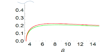
Figure 7: Signature changes in the induced metric $g_{\mu\nu}$ and effective metric $\gamma_{\mu\nu}$ for deformed $CP^{2}$ are given in the plot of $\tau$ versus $\tilde{\beta}$ in the region $ii)\;3.41\,\lesssim\,\tilde{\beta}$. A sign change in $g_{\theta\theta}$ or $\gamma_{\theta\theta}$ is indicated by the green curve. Sign changes in $g_{\tau\tau}$ or $\gamma_{\psi\psi}$ are indicated by the red and blue curves.

5.2.2 Effective metric

We next use (4.35) to compute the effective metric $\gamma_{\mu\nu}$ for deformed $CP^{2}$. Starting with the canonical Poisson brackets (4.6), we now obtain the following results for the nonvanishing components of the symplectic matrix $[\Theta^{\mu\nu}]$:

$$\Theta^{\tau\psi}=\frac{1}{\sin\tau\cos\tau}\qquad\Theta^{\theta\psi}=\frac{2\cot\theta}{\sin^{2}\tau}\qquad\Theta^{\theta\phi}=-\frac{2\csc\theta}{\sin^{2}\tau}$$ (5.100)

Computing determinants, we get

$$\det\Theta = \frac{4\csc^{2}\theta}{\cos^{2}\tau\sin^{6}\tau}$$ (5.101)

$$|\det\gamma||\det\Theta| = |\det g||\det\Theta|=4|g_{\tau\tau}|\,(\cos^{2}\tau-\mu^{2}\sin^{2}\tau)^{2}$$ (5.103)

As a result, the nonvanishing components of the effective metric tensor are

$$\frac{\gamma_{\tau\tau}}{\sqrt{|\det\gamma||\det\Theta|}} = -1$$ (5.104)

$$\frac{\gamma_{\theta\theta}}{\sqrt{|\det\gamma||\det\Theta|}} = \frac{1}{4(\mu^{2}-\cot^{2}\tau)}$$ (5.106)

$$\frac{\gamma_{\psi\psi}}{\sqrt{|\det\gamma||\det\Theta|}} = \frac{1}{4(\mu^{2}-\nu^{2}-{\rm sec}^{2}\tau\,{\rm csc}^{2}\tau)}\;,$$ (5.108)

in addition to $\gamma_{\phi\phi}=\gamma_{\psi\psi}\,\cos^{2}\theta+\gamma_{\theta\theta}\,\sin^{2}\theta$ and $\gamma_{\psi\phi}=\gamma_{\psi\psi}\,\cos\theta$. As with the deformed $CP^{1,1}$ and $CP^{0,2}$ solutions, signature changes in the effective metric coincide with signature changes in the induced metric. So like with the induced metric, the effective metric undergoes only one signature change when $\tilde{\beta}$ has the values in $i)$. It is a change from the Euclidean signature to one where the effective metric has two space-like directions and two time-like directions.

Also like with the induced metric, the effective metric undergoes three signature changes when $\tilde{\beta}$ has the values in $ii)$, which are indicated in figure seven. A sign change in $\gamma_{\theta\theta}$ occurs for $\tan\tau=\frac{1}{|\mu|}$ (indicated by the green curve in the figure), and sign changes in $\gamma_{\psi\psi}$ occur at $\sin 2\tau=\frac{2}{\sqrt{\mu^{2}-\nu^{2}}}$ (indicated by the red and blue curves in the figure). The effective metric has Euclidean signature below the red curve. In the tiny intermediate region between the red and green curves, the effective metric, like the induced metric, has two-space-like directions and two time-like directions. The effective metric has Lorentzian signature in the intermediate region between the green and blue curves, with $\tau$ being time-like. Above the blue curve, the induced metric has two-space-like directions and two time-like directions.

For the Lorentzian region, which we found between the green and blue curves in figure seven, the effective metric describes a closed space-time cosmology. For a fixed $\tilde{\beta}$ with values in $ii)$, the sign changes in $\gamma_{\psi\psi}$, depicted as red and blue curves in figure seven, correspond to space-time singularities. We denote the values of $\tau$ at these singularities by $\tau_{0}$ and $\tau_{1}$, with $\tau_{0}<\tau_{1}$. Which one of these is the initial singularity, and which one is the final singularity, of course, depends on the direction of time. We obtain the time evolution of the spacial scale for this region in the next subsection.

5.2.3 Expansion and contraction

In the previous section, we saw that the effective metric for deformed $CP^{2}$ can have Lorentzian signature when $\tilde{\beta}$ has the values in $ii)$. In this case, $\tau$ is the time-like coordinate, and it evolves from one signature change to another. From (5.94), $|\zeta_{1}|^{2}+|\zeta_{2}|^{2}=\tan^{2}\tau$, and so, like with the deformed $CP^{1,1}$ and $CP^{0,2}$ solutions, a $\tau$-slice of the four-dimensional manifold away from singularities is a three-sphere, or more precisely, a Berger sphere. We can compute the spatial scale $a(|\tau|)$ at any $\tau-$slice and proper time $t$ in the co-moving frame for the deformed $CP^{2}$ solution, using (5.61) and (5.64), respectively. For the former, we get

$$a(|\tau|)^{3}={(4\pi)^{2}\,|\sin^{4}\tau\cos\tau|\,|\cot^{2}\tau-\mu^{2}|^{\frac{1}{2}}\;|(\mu^{2}-\nu^{2})\sin^{2}\tau\cos^{2}\tau-1|^{\frac{1}{4}}}$$ (5.109)

It follows that the spatial scale vanishes at the signature changes, which are associated with the cosmological singularities. For the latter, (5.64) gives

$$t(\tau) = 2\,\int_{\tau_{0}}^{\tau}d\tau^{\prime}\,|\cos^{2}\tau^{\prime}-\mu^{2}\sin^{2}\tau^{\prime}|^{\frac{1}{2}}\;\Big{|}(\mu^{2}-\nu^{2})\sin^{2}\tau^{\prime}\cos^{2}\tau^{\prime}-1\Big{|}^{\frac{1}{4}}$$ (5.110)

The lower integration limit $\tau_{0}$ corresponds to the value of $\tau$ at the coordinate singularity defined by $\sin 2\tau_{0}=\frac{2}{\sqrt{\mu^{2}-\nu^{2}}}$, $\tau_{0}<\frac{\pi}{4}$, corresponding to the sign change in $\gamma_{\psi\psi}$. In figure eight, we plot $a(\tau)$ versus $t(\tau)$ for three values of $\tilde{\beta}$ in region $ii)$. For $\tau$ close to $\tau_{0}$, we get $a\sim(\tau-\tau_{0})^{\frac{1}{12}}$, $t\sim(\tau-\tau_{0})^{\frac{5}{4}}$, and hence, $a\sim t^{\frac{1}{15}}$. We find identical behavior near the other singularity at $\tau=\tau_{1}$. We thus get a very rapid initial expansion and a very rapid final contraction.

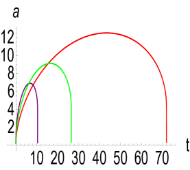
Figure 8: $a(\tau)$ versus $t(\tau)$ for the region of deformed $CP^{2}$ where the effective metric has Lorentzian signature, for $\tilde{\beta}=3.5$ (red curve), $3.75$ (green curve) and $5$ (purple curve).

6 Conclusions

We have obtained a number of new solutions to IKKT-type matrix models, which exhibit signature change in the commutative limit. All such examples found so far, including the non-commutative $H^{4}$ solution of [13], require including a mass term in the matrix action. Since mass terms result from an IR regularization,[16] it is interesting to speculate whether signature change on the brane is connected to the regularization. On the other hand, we remark that the mass term resulting from the regularization does not necessarily lead to signature change, since we have obtained solutions to the massive matrix model which exhibit no signature change in the commutative limit. For example, no sign changes occur in either the induced metric or effective metric for deformed $CP^{0,2}$ when $-1<\tilde{\beta}\lesssim-0.746$ and $-0.603\,\lesssim\,\tilde{\beta}\,\leq-.6\,$. Moreover, our work does not rule out the possibility of solutions to a massless matrix model which exhibit signature change in the commutative limit.

The four-dimensional solutions of section five are deformations of non-commutative complex projective spaces, specifically non-commutative $CP^{2}$, $CP^{1,1}$ and $CP^{0,2}$. The manifolds that emerge from these solutions can have multiple signature changes. The manifolds resulting from deformed non-commutative $CP^{0,2}$ solution can undergo two signature changes, while those resulting from deformed non-commutative $CP^{2}$ solution can have up to three signature changes. The regions where the effective metric of these manifolds have Lorentzian signature serve as crude models of closed (in the case of non-commutative $CP^{2}$) and open (in the case of non-commutative $CP^{1,1}$ and $CP^{0,2}$) cosmological space-times. They contain cosmological singularities that are resolved away from the commutative limit. The evolution of the spatial scale $a$ as a function of the proper time $t$ in the co-moving frame was computed for these examples. For all examples (and also the example of non-commutative $H^{4}$ in [13]) an extremely rapid expansion (or contraction, in case of the big crunch singularity of the closed cosmology) was found for the spacial scale $a$ near the cosmological singularities. Rather than following an exponential behavior, we obtained $a\sim t^{\frac{1}{15}}$ near $t=0$ for non-commutative $CP^{2}$ and $CP^{1,1}$, and $a\sim t^{\frac{1}{9}}$ for non-commutative $CP^{0,2}$. Also like non-commutative $H^{4}$,[13] the space-times emerging from the deformed non-commutative $CP^{1,1}$ and $CP^{0,2}$ solutions expand linearly at late times, $a\sim t$.

Unlike the space-time manifold that emerges from non-commutative $H^{4}$,[13] the manifolds that emerge from non-commutative $CP^{2}$, $CP^{1,1}$ and $CP^{0,2}$ are not maximally symmetric. For the latter manifolds, any time slice of the space-time is a Berger sphere. Although being, perhaps, less realistic than non-commutative $H^{4}$ with regards to cosmology, the examples of non-commutative $CP^{2}$, $CP^{1,1}$ and $CP^{0,2}$ are considerably simpler spaces than non-commutative $H^{4}$, with evidently similar outcomes for the evolution of the spatial scale. Non-commutative $H^{4}$ carries an additional bundle structure, that is not present for the solutions of section five. In order to close the algebra on non-commutative $H^{4}$, one must extend it to a larger non-commutative space. That space is non-commutative $CP^{1,2}$. In the commutative limit, one recovers the $CP^{1,2}$ manifold, an $S^{2}$ bundle over $AdS^{4}$.

The eight-dimensional matrix model considered in sections four and five utilized a particular indefinite background metric $\eta$, the $su(2,1)$ Cartan-Killing metric. Other indefinite background metrics can be considered. $\eta$=diag($+,+,+,+,+,+,+,-)$ was used in [12], to obtain non-commutative $CP^{2}$ solutions. We can preserve $SO(3)$ rotational symmetry with a generalization of the background metric to $\eta$=diag($\kappa_{3},\kappa_{3},\kappa_{3},-,-,-,-,\kappa_{8})$, $\kappa_{3},\kappa_{8}=\pm$. (We exclude $\kappa_{3}=\kappa_{8}=-$, since this will only produce a Euclidean induced and effective metric.) If for example, we search for deformed $CP^{1,1}$ and $CP^{0,2}$ solutions to the matrix equations (5.3) with this metric, then the conditions (5.14) generalize to

$$(2\mu-\alpha)\Bigl{(}\mu^{2}\kappa_{3}+\frac{1}{2}\Bigr{)}+3\mu\tilde{\beta} = 0$$ (6.1)

$$\mu^{2}\kappa_{3}+\nu^{2}\kappa_{8}+2-\alpha(\mu\kappa_{3}+\nu\kappa_{8})+4\tilde{\beta} = 0$$ (6.3)

$$2\nu-\alpha+2\nu\tilde{\beta} = 0$$ (6.5)

where we again assumed the ansatz (5.9). Solutions for different choices of $\kappa_{3}$ and $\kappa_{8}$ may be found, although they may be quite nontrivial, and many more four-dimensional signature changing manifolds are expected to emerge in the commutative limit.

In this article we have neglected stability issues, and the addition of fermions. The question of stable solutions to matrix models is highly non-trivial. For two-dimensional solutions it was found previously that longitudinal and transverse fluctuations contribute with opposite signs to the kinetic energy. It is unclear how the extension to a fully supersymmetric theory can resolve this issue. We hope to address such questions in the future.

Appendix A      Some properties of $su(2,1)$ in the defining representation

In terms of $su(3)$ Gell-Mann matrices $\lambda_{a}$, the $su(2,1)$ Gell-Mann matrices $\tilde{\lambda}_{a}$ are given by

$$\tilde{\lambda}_{\tt a} = \lambda_{\tt a}\;,\qquad\;\;{\tt a}=1,2,3,8$$ (A.1)

$$\tilde{\lambda}_{\tt a^{\prime}} = i\lambda_{\tt a^{\prime}}\;,\qquad{\tt a^{\prime}}=4,5,6,7$$ (A.3)

They satisfy the hermiticity properties (4.7).

The structure constants for $su(2,1)$ are $C_{ab}^{\;\;\;c}=\tilde{f}_{abd}\eta^{dc}$, where $\eta_{ab}$ is the Cartan-Killing metric (4.9), and $\tilde{f}_{abc}$ are totally antisymmetric, with the nonvanishing values

$$\tilde{f}_{123}=1\qquad\qquad\qquad\tilde{f}_{845}=\tilde{f}_{867}=-\frac{\sqrt{3}}{2}$$ (A.4)

(A.5)

$$\tilde{f}_{147}=\tilde{f}_{165}=\tilde{f}_{246}=\tilde{f}_{257}=\tilde{f}_{345}=\tilde{f}_{376}=-\frac{1}{2}$$ (A.6)

Except for $\tilde{f}_{123}$ these structure constants are opposite in sign from those obtained from the standard Gell-Mann matrices of $su(3)$.

Some useful identities for the $su(2,1)$ Gell-Mann matrices and $\tilde{f}_{abc}$ are

$${\rm tr}\,\tilde{\lambda}_{a}\tilde{\lambda}_{b} = [\tilde{\lambda}_{a}]^{i}_{\;\,j}[\tilde{\lambda}_{b}]^{j}_{\;\,i}\;=\;2\eta_{ab}\;,$$ (A.7)

$$[\tilde{\lambda}_{a},\tilde{\lambda}_{b}]_{+} = 2\tilde{d}_{abc}\tilde{\lambda}^{c}+\frac{4}{3}\eta_{ab}{\rm 1\!l}$$ (A.9)

$$\tilde{f}_{abc}\tilde{f}^{bc}_{\;\;\;d} = 3\eta_{ad}$$ (A.11)

$$[\tilde{\lambda}^{a}]^{i}_{\;\,j}[\tilde{\lambda}_{a}]^{k}_{\;\,\ell} = 2\delta^{i}_{\ell}\delta^{k}_{j}-\frac{2}{3}\delta^{i}_{j}\delta^{k}_{\ell}$$ (A.13)

$[\;,\;]_{+}$ denotes the anti-commutator, and $\tilde{d}_{abc}$ are totally symmetric, with the nonvanishing values

$$\tilde{d}_{443}=\tilde{d}_{553}=\tilde{d}_{146}=\tilde{d}_{157}=\tilde{d}_{256}=-\frac{1}{2}\qquad\tilde{d}_{663}=\tilde{d}_{773}=\tilde{d}_{247}=\frac{1}{2}$$ (A.14)

(A.15)

$$\tilde{d}_{118}=\tilde{d}_{228}=\tilde{d}_{338}=\frac{1}{\sqrt{3}}\qquad\tilde{d}_{448}=\tilde{d}_{558}=\tilde{d}_{668}=\tilde{d}_{778}=\frac{1}{2\sqrt{3}}\qquad\tilde{d}_{888}=-\frac{1}{\sqrt{3}}$$ (A.16)

(A.13) is the Fierz identity, which has the same form as that for $su(3)$.

Appendix B      Effective metric

Here we review the derivation of (4.35), relating the effective metric $\gamma_{\mu\nu}$ to the induced metric $g_{\mu\nu}$. We use the example of the massless scalar field.[15] We then apply the result to compute the effective metrics for (undeformed) $CP^{1,1}$ and $CP^{0,2}$.

Denote the scalar field by $\Phi=\Phi(X)$ on a non-commutative background spanned by matrices $X_{a}$. The standard action is

$$-\frac{1}{2k^{2}}{\rm Tr}[X_{a},\Phi][X^{a}\Phi]\;,$$ (B.1)

$a=1,2,...,d$. Now take the semi-classical limit $\hbar\rightarrow 0$. This means again replacing matrices $X_{a}$ by commuting variables $x_{a}$, corresponding to embedding coordinates of some continuous manifold. $\Phi$ is then replaced by a function $\phi$ on the manifold, and commutators are replaced by $i\hbar$ times Poisson brackets. We also need to replace the trace by an integration $\int d\mu(x)$, where $d\mu(x)$ is an invariant integration measure. Say that the manifold is parametrized by $\sigma=(\sigma^{1},\sigma^{2},...,\sigma^{n})$, $n\leq d$, with symplectic two-form $\Omega=\frac{1}{2}[\Theta^{-1}]_{\mu\nu}\,d\sigma^{\mu}\wedge d\sigma^{\nu}$. Then one can set $d\mu(x)=\frac{d\sigma}{\sqrt{|\det\Theta|}}$. Taking $k\rightarrow\hbar\kappa$, the semi-classical limit of (B.1) is

$$-\frac{1}{2{\kappa}^{2}}\int\frac{d\sigma}{\sqrt{|\det\Theta|}}\,\{x_{a},\phi\}\{x^{a},\phi\}$$ (B.2)

$$= -\frac{1}{2{\kappa}^{2}}\int\frac{d\sigma}{\sqrt{|\det\Theta|}}\,\Theta^{\rho\mu}\partial_{\rho}x_{a}\partial_{\mu}\phi\;\Theta^{\sigma\nu}\partial_{\sigma}x^{a}\partial_{\nu}\phi$$ (B.4)

$$= -\frac{1}{2{\kappa}^{2}}\int\frac{d\sigma}{\sqrt{|\det\Theta|}}\,\Theta^{\rho\mu}g_{\rho\sigma}\Theta^{\sigma\nu}\,\partial_{\mu}\phi\partial_{\nu}\phi\;$$ (B.6)

On the other hand, the standard action of a scalar field $\phi$ on a background metric $\gamma_{\mu\nu}$ is

$$-\frac{1}{2{\kappa}^{2}}\int d\sigma{\sqrt{|\det\gamma|}}\gamma^{\mu\nu}\partial_{\mu}\phi\partial_{\nu}\phi$$ (B.7)

Identifying these two actions gives (4.35).

As examples, we compute the effective metrics for (undeformed) $CP^{1,1}$ and $CP^{0,2}$, and show that they are identical to the corresponding induced metrics.

1. Effective metric for $CP^{1,1}\,.\;$ Using (4.29), the nonvanishing components $\Theta^{\mu\nu}$ for $CP^{1,1}$ are

   $$\Theta^{\tau\psi}=\frac{1}{\cosh\tau\sinh\tau}\qquad\quad\Theta^{\theta\psi}=\frac{2\cot\theta}{\cosh^{2}\tau}\qquad\quad\Theta^{\theta\phi}=-\frac{2\csc\theta}{\cosh^{2}\tau}$$ (B.8)

   Then

   $$\det\Theta=\frac{4\csc^{2}\theta}{\sinh^{2}\tau\cosh^{6}\tau}\quad\qquad\quad|\det\gamma|=4\cosh^{6}\tau\sinh^{2}\tau\sin^{2}\theta$$ (B.9)

   Computing $\Theta^{T}g\Theta$ we find the following nonvanishing components

   $$[\Theta^{T}g\Theta]^{\tau\tau}=-1\qquad\quad[\Theta^{T}g\Theta]^{\theta\theta}=\frac{4}{\cosh^{2}\tau}\qquad\quad[\Theta^{T}g\Theta]^{\phi\phi}=\frac{4\csc^{2}\theta}{\cosh^{2}\tau}$$

   $$[\Theta^{T}g\Theta]^{\psi\psi}=\frac{4(\cot^{2}\theta-{\rm csch}^{2}\tau)}{\cosh^{2}\tau}\qquad\quad[\Theta^{T}g\Theta]^{\phi\psi}=-\frac{4\cot\theta\csc\theta}{\cosh^{2}\tau}$$ (B.10)

   Using (4.35) and (B.9), we then get $\gamma_{\mu\nu}=g_{\mu\nu}$.

2. Effective metric for $CP^{0,2}\,.\;$ Using (4.34) the nonvanishing components $\Theta^{\mu\nu}$ for $CP^{0,2}$ are

   $$\Theta^{\tau\psi}=\frac{1}{\cosh\tau\sinh\tau}\qquad\quad\Theta^{\theta\psi}=\frac{2\cot\theta}{\sinh^{2}\tau}\qquad\quad\Theta^{\theta\phi}=-\frac{2\csc\theta}{\sinh^{2}\tau}$$ (B.11)

   Here

   $$\det\Theta=\frac{4\csc^{2}\theta}{\sinh^{6}\tau\cosh^{2}\tau}\quad\qquad|\det\gamma|=4\cosh^{2}\tau\sinh^{6}\tau\sin^{2}\theta\quad$$ (B.12)

   The nonvanishing components of $\Theta^{T}g\Theta$ are

   $$[\Theta^{T}g\Theta]^{\tau\tau}=-1\qquad\quad[\Theta^{T}g\Theta]^{\theta\theta}=\frac{-4}{\sinh^{2}\tau}\qquad\quad[\Theta^{T}g\Theta]^{\phi\phi}=\frac{-4\csc^{2}\theta}{\sinh^{2}\tau}$$

   $$[\Theta^{T}g\Theta]^{\psi\psi}=\frac{-4(\cot^{2}\theta+{\rm sech}^{2}\tau)}{\sinh^{2}\tau}\qquad\quad[\Theta^{T}g\Theta]^{\phi\psi}=\frac{4\cot\theta\csc\theta}{\sinh^{2}\tau}$$ (B.13)

   Using (4.35) and (B.12), we once again get $\gamma_{\mu\nu}=g_{\mu\nu}$.

Acknowledgements

A.S. is grateful for useful discussions with J. Hoppe, H. Kawai, S. Kurkcuoglu and H. Steinacker, and wishes to thank the members of the Erwin Schrödinger International Institute for their hospitality and support during the Workshop on “Matrix Models for non-commutative Geometry and String Theory”.

References

- [1] D. Atkatz and H. Pagels, “The Origin of the Universe as a Quantum Tunneling Event,” Phys. Rev. D 25, 2065 (1982).
- [2] A. Vilenkin, “Creation of Universes from Nothing,” Phys. Lett. 117B, 25 (1982).
- [3] A. D. Sakharov, “Cosmological Transitions With a Change in Metric Signature,” Sov. Phys. JETP 60, 214 (1984) [Zh. Eksp. Teor. Fiz. 87, 375 (1984)] [Sov. Phys. Usp. 34, 409 (1991)].
- [4] G. W. Gibbons and J. B. Hartle, “Real Tunneling Geometries and the Large Scale Topology of the Universe,” Phys. Rev. D 42, 2458 (1990).
- [5] T. Dray, C. A. Manogue and R. W. Tucker, “Particle production from signature change,” Gen. Rel. Grav. 23, 967 (1991).
- [6] M. Mars, J. M. M. Senovilla and R. Vera, “Signature change on the brane,” Phys. Rev. Lett. 86, 4219 (2001).
- [7] J. Mielczarek, “Signature change in loop quantum cosmology,” Springer Proc. Phys. 157, 555 (2014); J. Mielczarek and T. Trześniewski, “Spectral dimension with deformed spacetime signature,” Phys. Rev. D 96, no. 2, 024012 (2017).
- [8] J. Ambjorn, D. N. Coumbe, J. Gizbert-Studnicki and J. Jurkiewicz, “Signature Change of the Metric in CDT Quantum Gravity?,” JHEP 1508, 033 (2015).
- [9] A. Barrau and J. Grain, “Cosmology without time: What to do with a possible signature change from quantum gravitational origin?,” arXiv:1607.07589 [gr-qc].
- [10] M. Bojowald and S. Brahma, “Signature change in loop quantum gravity: General midisuperspace models and dilaton gravity,” arXiv:1610.08840 [gr-qc].
- [11] A. Chaney, L. Lu and A. Stern, “Lorentzian Fuzzy Spheres,” Phys. Rev. D 92, no. 6, 064021 (2015).
- [12] A. Chaney and A. Stern, “Fuzzy spacetimes,” Phys. Rev. D 95, no. 4, 046001 (2017).
- [13] H. C. Steinacker, “Cosmological space-times with resolved Big Bang in Yang-Mills matrix models,” JHEP 1802, 033 (2018); H. C. Steinacker, “Quantized open FRW cosmology from Yang-Mills matrix models,” Phys. Lett. B 782, 176 (2018); M. Sperling and H. C. Steinacker, “The fuzzy 4-hyperboloid and higher-spin in Yang-Mills matrix models,” arXiv:1806.05907 [hep-th].
- [14] N. Ishibashi, H. Kawai, Y. Kitazawa and A. Tsuchiya, “A Large N reduced model as superstring,” Nucl. Phys. B 498, 467 (1997).
- [15] For an introduction see, H. Steinacker, “Emergent Geometry and Gravity from Matrix Models: an Introduction,” Class. Quant. Grav. 27, 133001 (2010).
- [16] S. W. Kim, J. Nishimura and A. Tsuchiya, “Expanding (3+1)-dimensional universe from a Lorentzian matrix model for superstring theory in (9+1)-dimensions,” Phys. Rev. Lett. 108, 011601 (2012); “Expanding universe as a classical solution in the Lorentzian matrix model for nonperturbative superstring theory,” Phys. Rev. D 86, 027901 (2012).
- [17] C. Gu, “The extremal surfaces in 3-dimensional Minkowski space,” Acta. Math. Sinica. 1, 173 (1985).
- [18] V. A. Klyachin, “Zero mean curvature surfaces of mixed type in Minkowski space,” Izv. Math. 67, 209 (2003).
- [19] Y. W. Kim and S.-D. Yang, “Prescribing singularities of maximal surfaces via a singular Björling representation formula,” J. Geom. Phys. 57, 2167 (2007).
- [20] Y. W. Kim, S.-E. Koh, H. Shin and S.-D. Yang, “Spacelike maximal surfaces, timelike minimal surfaces, and Björling representation formulae,” J. of Korean Math. Soc. 48, 1083 (2011).
- [21] S. Fujimori, Y. W. Kim, S.-E. Koh, W. Rossman, H. Shin, M. Umehara, K. Yamada, and S.-D. Yang, “Zero mean curvature surfaces in Lorentz–Minkowski 3-space which change type across a light-like line,” Osaka J. Math. 52, 285 (2015).
- [22] P. M. Ho and M. Li, “Large N expansion from fuzzy AdS(2),” Nucl. Phys. B 590, 198 (2000); “Fuzzy spheres in AdS / CFT correspondence and holography from noncommutativity,” Nucl. Phys. B 596, 259 (2001).
- [23] D. Jurman and H. Steinacker, “2D fuzzy Anti-de Sitter space from matrix models,” arXiv:1309.1598 [hep-th].
- [24] A. Stern, “Matrix Model Cosmology in Two Space-time Dimensions,” Phys. Rev. D 90, no. 12, 124056 (2014).
- [25] A. Chaney, L. Lu and A. Stern, “Matrix Model Approach to Cosmology,” Phys. Rev. D 93, no. 6, 064074 (2016).
- [26] A. Pinzul and A. Stern, “Non-commutative duality: the case of massless scalar fields,” Phys. Rev. D 96, no. 6, 066019 (2017).
- [27] M. Chaichian, A. Demichev, P. Presnajder and A. Tureanu, “Space-time noncommutativity, discreteness of time and unitarity,” Eur. Phys. J. C 20, 767 (2001); “non-commutative quantum field theory: Unitarity and discrete time,” Phys. Lett. B 515, 426 (2001).
- [28] A. P. Balachandran, T. R. Govindarajan, A. G. Martins and P. Teotonio-Sobrinho, “Time-space noncommutativity: Quantised evolutions,” JHEP 0411, 068 (2004).
- [29] A. Stern, “Noncommutative Static Strings from Matrix Models,” Phys. Rev. D 89, no. 10, 104051 (2014) [arXiv:1404.2549 [hep-th]].
- [30] V. P. Nair and S. Randjbar-Daemi, “On brane solutions in M(atrix) theory,” Nucl. Phys. B 533, 333 (1998).
- [31] G. Alexanian, A. P. Balachandran, G. Immirzi and B. Ydri, “Fuzzy CP**2,” J. Geom. Phys. 42, 28 (2002).
- [32] A. P. Balachandran, B. P. Dolan, J. H. Lee, X. Martin and D. O’Connor, “Fuzzy complex projective spaces and their star products,” J. Geom. Phys. 43, 184 (2002).
- [33] T. Azuma, S. Bal, K. Nagao and J. Nishimura, “Dynamical aspects of the fuzzy CP**2 in the large N reduced model with a cubic term,” JHEP 0605, 061 (2006).
- [34] D. Karabali, V. P. Nair and S. Randjbar-Daemi, “Fuzzy spaces, the M(atrix) model and the quantum Hall effect,” In *Shifman, M. (ed.) et al.: From fields to strings, vol. 1* 831-875.
- [35] H. Grosse and H. Steinacker, “Finite gauge theory on fuzzy CP**2,” Nucl. Phys. B 707, 145 (2005)
- [36] A. P. Balachandran, S. Kurkcuoglu and S. Vaidya, “Lectures on fuzzy and fuzzy SUSY physics,” Singapore, Singapore: World Scientific (2007) 191 p.
- [37] K. Hasebe, “Non-Compact Hopf Maps and Fuzzy Ultra-Hyperboloids,” Nucl. Phys. B 865, 148 (2012) .
- [38] J. Arnlind and J. Hoppe, “The world as quantized minimal surfaces,” Phys. Lett. B 723, 397 (2013).