Stroboscopic Tests for Thermalization of Electrons in Pump/Probe Experiments

Abstract

One of the goals of pump/probe spectroscopies is to determine how electrons relax after they have been driven out of equilibrium. It is challenging to determine how close electrons are to a thermal state solely by fitting their distribution to a Fermi-Dirac distribution. Instead, we propose that one compare the effective temperatures of both fermions and collective bosonic modes (derived from the fermions) to determine the distance from a thermal state. Measurements of effective fermionic and bosonic temperatures can be achieved directly via photoemission and nonresonant Raman scattering. Their difference quantifies the distance from thermal equilibrium.

Time-resolved pump/probe experiments are commonly used to examine the nonequilibrium dynamics of different excitations in solids Hsieh et al. (2012); Hellmann et al. (2010); Perfetti et al. (2006); Wegkamp et al. (2014); Smallwood et al. (2016a); Giannetti et al. (2016). Two of the most common spectroscopies measured in these experiments are optical conductivity and photoemission spectroscopy. Here we focus on how another spectroscopy—nonresonant electronic Raman scattering—can be combined with photoemission to determine proximity of the electrons to thermal equilibrium. It is well known that thermometry of electrons is challenging in ultrafast experiments and often is performed by fitting to a Fermi-Dirac distribution function. Experimentally, nonequilibrium Raman scattering has been measured for phonons in graphite Yang et al. (2017) and combined with photoemission of electrons to study the thermal relaxation of both. Here, we develop the theory for nonresonant electronic Raman scattering in the $B_{\text{1g}}$ symmetry channel and combine it with the known methods for photoemission to compare the two different effective temperatures. We perform our calculations for the spinless Falicov-Kimball model Falicov and Kimball (1969) within the nonequilibrium extension Freericks et al. (2006) of dynamical mean-field theory (DMFT) Brandt and Mielsch (1989); Freericks and Zlatić (2003). The model describes a strongly correlated metal-Mott-insulator transition, which occurs at the critical Coulomb interaction $U_{c}=\sqrt{2}$ when the system is at half filling.

In a pump-probe setup with a nonequilibrium pump and finite width probes, we adapt the formalism proposed by Nozières and Abrahams Nozières and Abrahams (1974) for resonant inelastic X-ray scattering (RIXS) to nonresonant electronic Raman scattering. The quantum system evolves from $t_{1}$ to $t_{2}$ via the evolution operator $U(t_{2},t_{1})=\mathcal{T}_{t}\exp{\bigl{\{}-i\int^{t_{2}}_{t_{1}}d\tilde{t}\mathcal{H}(\tilde{t})\bigr{\}}}$. Initially ($t\to-\infty$), the system is in an equilibrium state $|n\rangle$, which is an eigenstate of the initial (electronic) Hamiltonian $\mathcal{H}_{0}=\mathcal{H}(t\to-\infty)$. The system has two electric fields applied to it. The pump, which is treated semiclassically and the probe, which is treated quantum mechanically and perturbatively. The full system at arbitrary time $t$ is then

$$|\psi(t)\rangle=U(t,-\infty)|n\rangle\otimes a_{\mathbf{k}_{i},\mathbf{e}_{i}}^{\dagger}|0\rangle$$

$$=\mathcal{T}_{t}\exp{\biggl{\{}-i\int^{t}_{-\infty}d\tilde{t}(\mathcal{H}_{\text{loc}}+\mathcal{H}_{t}(\tilde{t}))\biggr{\}}}|n\rangle\otimes a_{\mathbf{k}_{i},\mathbf{e}_{i}}^{\dagger}|0\rangle,$$ (1)

where $a_{\mathbf{k}_{i},\mathbf{e}_{i}}^{{\dagger}}$ creates an incident photon with momentum ${\mathbf{k}_{i}}$, energy $\omega_{i}$, and polarization $\mathbf{e}_{i}$. The electronic Hamiltonian has two parts—$\mathcal{H}_{\text{loc}}=\sum_{i}[Un_{ic}n_{if}-\mu n_{ic}+E_{f}n_{if}]$ includes the local interaction $U$ between itinerant ($c$) and localized ($f$) electrons (and their chemical potentials) and the time-dependent part of the Hamiltonian $\mathcal{H}_{t}(t)$ describes the interaction with the total electric field (via the Peierls’ substitution to the hopping term):

$$\mathcal{H}_{t}(t)=-\sum\limits_{\langle i,j\rangle}\frac{t^{*}}{2\sqrt{D}}e^{-i\int^{\mathbf{R}_{j}}_{\mathbf{R}_{i}}d\mathbf{r}\cdot\mathbf{A}(r,t)}c^{{\dagger}}_{i}c_{j}^{\phantom{\dagger}}.$$ (2)

Here $n_{ic}=c_{i}^{\dagger}c_{i}^{\phantom{\dagger}}$ is the itinerant electron number operator and $n_{if}$ is the localized electron number operator; we work in the infinite-dimensional limit, where $D\rightarrow\infty$ with $t^{*}$ remaining finite. The hopping is between nearest neighbor sites $i$ and $j$. We assume that the electric field is spatially uniform, pointing along the diagonal, with $A(r,t)=A(t)$ the component in each spatial direction, and we ignore magnetic field and relativistic effects. The vector potential in the Hamiltonian gauge then produces the total electric field through $\mathbf{E}_{\text{tot}}(t)=-d\mathbf{A}(t)/dt$ (we set $\hbar=c=e=a=1$).

This vector potential has two terms $\mathbf{A}(t)=\mathbf{A}_{\text{pump}}(t)+\mathbf{A}_{\text{probe}}(t)$. We model the pump field by

$$\mathbf{E}_{\text{{pump}}}(t)=\mathbf{E}_{0}\cos{[\omega_{p}(t-t_{p})]}e^{-\frac{(t-t_{p})^{2}}{\sigma_{p}^{2}}},$$ (3)

where $\mathbf{E}_{0}$ is the magnitude of the pump field at time $t=t_{p}$, and $\omega_{p}$ and $\sigma_{p}$ define the frequency and width of the pump pulse, respectively.

Electronic Raman scattering is a second-order process, so we find resonant and nonresonant terms that are second order in the probe vector potential $\mathbf{A}_{\text{probe}}(t)$ Shastry and Shraiman (1990); Freericks and Devereaux (2001a); Shvaika et al. (2004, 2005); Devereaux and Hackl (2007). We will only work with the nonresonant contribution here. Summing over all the quantum states between the start and the end of the experiment, we end up with the final state in Eq. (Stroboscopic Tests for Thermalization of Electrons in Pump/Probe Experiments)

$$|\psi(\infty)\rangle=\frac{1}{2}\int^{\infty}_{-\infty}d\tilde{t}U_{\text{pump}}(t_{\text{exp}},\tilde{t})A^{\alpha}_{\text{probe}}(\tilde{t})$$

$$~{}~{}\times\gamma_{\alpha\beta}(\tilde{t})A^{\beta}_{\text{probe}}(\tilde{t})U_{\text{pump}}(\tilde{t},-\infty)|n\rangle\otimes a_{\mathbf{k}_{i},\mathbf{e}_{i}}^{\dagger}|0\rangle,$$ (4)

where the stress tensor operator in the momentum representation is $\gamma_{\alpha\beta}(t)=\sum_{k}\frac{\partial^{2}\epsilon(\mathbf{k},t)}{\partial k_{\alpha}\partial k_{\beta}}c_{\mathbf{k}}^{{\dagger}}c_{\mathbf{k}}^{\phantom{\dagger}}$, with a time-dependent electronic band energy $\epsilon(\mathbf{k},t)=-\frac{t^{*}}{\sqrt{D}}\sum_{\alpha=1}^{D}\cos{[k_{\alpha}-A^{\alpha}_{\text{pump}}(t)]}$ (the repeated indices $\alpha$ and $\beta$ are summed over). The probe field $A_{\text{probe}}^{\alpha}(t)=s(t)\sum_{\mathbf{k},\mathbf{e}}(\frac{2\pi}{\omega_{\mathbf{k}}})^{1/2}e_{\alpha}(e^{i\omega_{\mathbf{k}}t}a_{\mathbf{k},\mathbf{e}}^{{\dagger}}+e^{-i\omega_{\mathbf{k}}t}a_{\mathbf{k},\mathbf{e}})^{\phantom{\dagger}}$, which acts in the photon space, describes the creation and annihilation of photons with polarization $\mathbf{e}$, and frequency $\omega_{\mathbf{k}}$. The time profile of the probe pulse is defined by an envelope function $s(t)$, which we take to be $s(t)=\exp{[-(t-t_{0})^{2}/\sigma^{2}_{\text{b}}]}/(\sigma_{\text{b}}\sqrt{\pi})$ centered on time $t_{0}$ (which defines time delay of the probe). The width of the probe pulse is $\sigma_{\text{b}}$. The operator $U_{\text{pump}}(t_{2},t_{1})$ is the evolution operator in Eq. (Stroboscopic Tests for Thermalization of Electrons in Pump/Probe Experiments), but without the probe pulse.

The scattering amplitude is defined by the probability to find a photon with energy $\omega_{f}$ and polarization $\mathbf{e}_{f}$ in the final state given in Eq. (Stroboscopic Tests for Thermalization of Electrons in Pump/Probe Experiments). This is then weighted by the thermal factors and summed over all the equilibrium states. The electronic Raman scattering probability becomes

$$R(\omega_{i}-\omega_{f},t_{0})=\sum\limits_{n}\frac{e^{-\beta E_{n}}}{\mathcal{Z}}\langle\psi(\infty)|a_{\mathbf{k}_{f},\mathbf{e}_{f}}^{{\dagger}}a_{\mathbf{k}_{f},\mathbf{e}_{f}}^{\phantom{\dagger}}|\psi(\infty)\rangle,$$ (5)

where $\mathcal{Z}=\operatorname{Tr}\exp{(-\beta\mathcal{H}_{0})}$ is the partition function at the initial temperature $T=1/\beta$, and one needs to calculate an expectation value for the scattering probability over the photon vacuum state $|0\rangle$. Applying the Kadanoff-Baym-Keldysh formalism Kadanoff and Baym (1962); Keldysh (1965) we introduce Green’s functions which are built on two stress tensor operators $R^{c}_{\gamma\gamma}(t,t^{\prime})=-i\operatorname{Tr}\exp{(-\beta\mathcal{H}_{0})}\mathcal{T}_{c}\gamma(t)\gamma(t^{\prime})/\mathcal{Z}$ with times $t$ and $t^{\prime}$ being ordered on the contour. In the same way as it was done by Nozières and Abrahams Nozières and Abrahams (1974) for RIXS, one can show that this greater Green’s function defines the electronic Raman scattering probability $R(\Omega,t_{0})$ when the two times $t$ and $t^{\prime}$ are placed on different branches of the contour with $t$ ahead of $t^{\prime}$:

$$R^{>}_{\gamma\gamma}(t,t^{\prime})=-i\frac{1}{\mathcal{Z}}\operatorname{Tr}e^{-\beta\mathcal{H}_{0}}\gamma(t)\gamma(t^{\prime}).$$ (6)

Diagrammatically, the greater function $R^{>}_{\gamma\gamma}(t,t^{\prime})$ consists of the bare and renormalized bubbles, which are constructed from the greater $G^{>}_{k}(t,t^{\prime})=-i\operatorname{Tr}\exp{(-\beta\mathcal{H}_{0})}c_{k}^{\phantom{{\dagger}}}(t)c_{k}^{{\dagger}}(t^{\prime})/\mathcal{Z}$ and the lesser $G^{<}_{k}(t,t^{\prime})=i\operatorname{Tr}\exp{(-\beta\mathcal{H}_{0})}c_{k}^{{\dagger}}(t^{\prime})c_{k}^{\phantom{{\dagger}}}(t)/\mathcal{Z}$ momentum-dependent single-particle Green’s functions. The vertices of the bubbles include the factor $\bar{\gamma}(\mathbf{k},t)=\sum_{\alpha\beta}e_{i\alpha}\frac{\partial^{2}\epsilon(\mathbf{k}-\mathbf{A}_{\text{pump}}(t))}{\partial k_{\alpha}\partial k_{\beta}}e_{f\beta}$. We consider $B_{\text{1g}}$ symmetry only, so the polarization vectors of the incident and scattered photons are equal to $\mathbf{e}_{i}=(1,1,1,...)$ and $\mathbf{e}_{f}=(-1,1,-1,...)$, respectively. In the case of nearest neighbor hopping, we find $\bar{\gamma}_{B_{\text{1g}}}(\mathbf{k},t)=\sum_{\alpha=1}^{D}(-1)^{\alpha}\cos{[k_{\alpha}-A^{\alpha}_{\text{pump}}(t)]}/{\sqrt{D}}$. Due to this form of the stress tensor and the local character of the irreducible charge vertex Zlatic and Horvatic (1990), the renormalized bubble vanishes Freericks and Devereaux (2001b); Shvaika et al. (2005) and we end up with the bare bubble only.

We perform the summation over momenta $\mathbf{k}$ by integrating over energy with the joint density of states $\rho(\epsilon)\rho(\bar{\epsilon})$, which is the product of the Gaussians given by $\rho(\epsilon)=\exp{(-\epsilon^{2})}/\sqrt{\pi}$ and $\bar{\epsilon}=\bar{\epsilon}(\mathbf{k})=-\sum_{\alpha=1}^{D}\sin k_{\alpha}/\sqrt{D}$ Freericks and Devereaux (2001b, a). Finally, we perform the Fourier transform from time to frequency and we obtain [after suppressing the overall “scattering strength” prefactor $4\pi^{2}/(\omega_{i}\omega_{f})$]:

$$R_{B_{\text{1g}}}^{N}(\Omega,t_{0})=\frac{1}{2}\operatorname{Re}\int\!dt\!\int\!dt^{\prime}s^{2}(t)s^{2}(t^{\prime})e^{i\Omega(t-t^{\prime})}\cos{[A_{\text{pump}}(t)-A_{\text{pump}}(t^{\prime})]}\int\!d\epsilon\!\int\!d\bar{\epsilon}\rho(\epsilon)\rho(\bar{\epsilon})G_{\epsilon,\bar{\epsilon}}^{>}(t,t^{\prime})G_{\epsilon,\bar{\epsilon}}^{<}(t^{\prime},t)$$ (7)

with $\Omega=\omega_{i}-\omega_{f}$ being the frequency shift for the scattered photons. Note that this is a general DMFT result, independent of the choice of Hamiltonian.

In equilibrium and for the monochromatic light beams ($s(t)\to$ constant), the Stokes and anti-Stokes lines of the Raman cross section are connected by the relation $R_{B_{\text{1g}}}^{N}(\Omega)/R_{B_{\text{1g}}}^{N}(-\Omega)=e^{\beta\Omega}$, for $\Omega>0$. When a probe pulse is present, this relation is replaced by a similar one with a displaced frequency $\tilde{\Omega}=\Omega-\frac{\beta}{\sigma_{b}^{2}}$ Shvaika et al. (2018)

$$\frac{R_{B_{\text{1g}}}^{N}(\tilde{\Omega}-\frac{\beta}{\sigma_{b}^{2}},t_{0})}{R_{B_{\text{1g}}}^{N}(-\tilde{\Omega}-\frac{\beta}{\sigma_{b}^{2}},t_{0})}=e^{\beta\tilde{\Omega}}.$$ (8)

We have found from our numerics, that in a wide enough region of $\tilde{\Omega}\approx 0$, the value of the ratio in Eq. (8) holds and can be used to estimate the effective temperature $\beta_{\text{eff}}=1/T_{\text{eff}}$ of the two-particle excitations during the nonequilibrium process. Motivated by Yang et al. (2017), we can compare this “two-particle” temperature, with an effective “single-particle” temperature extracted from the time-resolved photoemission spectra (tr-PES). The tr-PES spectral function is defined by the local lesser Green’s function as follows Freericks et al. (2009):

$$P^{<}(\omega,t_{0})=-i\int\!dt\!\int\!dt^{\prime}s(t)s(t^{\prime})e^{-i\omega(t-t^{\prime})}G^{<}_{\text{loc}}(t,t^{\prime});$$ (9)

the local Green’s function is found from the momentum-dependent Green’s function by summing over all momenta with equal weight. As an analogy to the equilibrium case, we define the nonequilibrium density-of-states via the probe-envelope-modified retarded response function:

$$A_{d}(\omega,t_{0}) =i\int dt\int dt^{\prime}s(t)s(t^{\prime})e^{-i\omega(t-t^{\prime})}$$

$$\times\theta(t-t^{\prime})[G^{>}_{\text{loc}}(t,t^{\prime})-G^{<}_{\text{loc}}(t,t^{\prime})].$$ (10)

The ratio of the tr-PES spectral function to density-of-states is used to determine the nonequilibrium distribution function for the fermionic states Smallwood et al. (2016b); Stafford (2016) $f_{s}(\omega,t_{0})=P^{<}(\omega,t_{0})/A_{d}(\omega,t_{0})$.

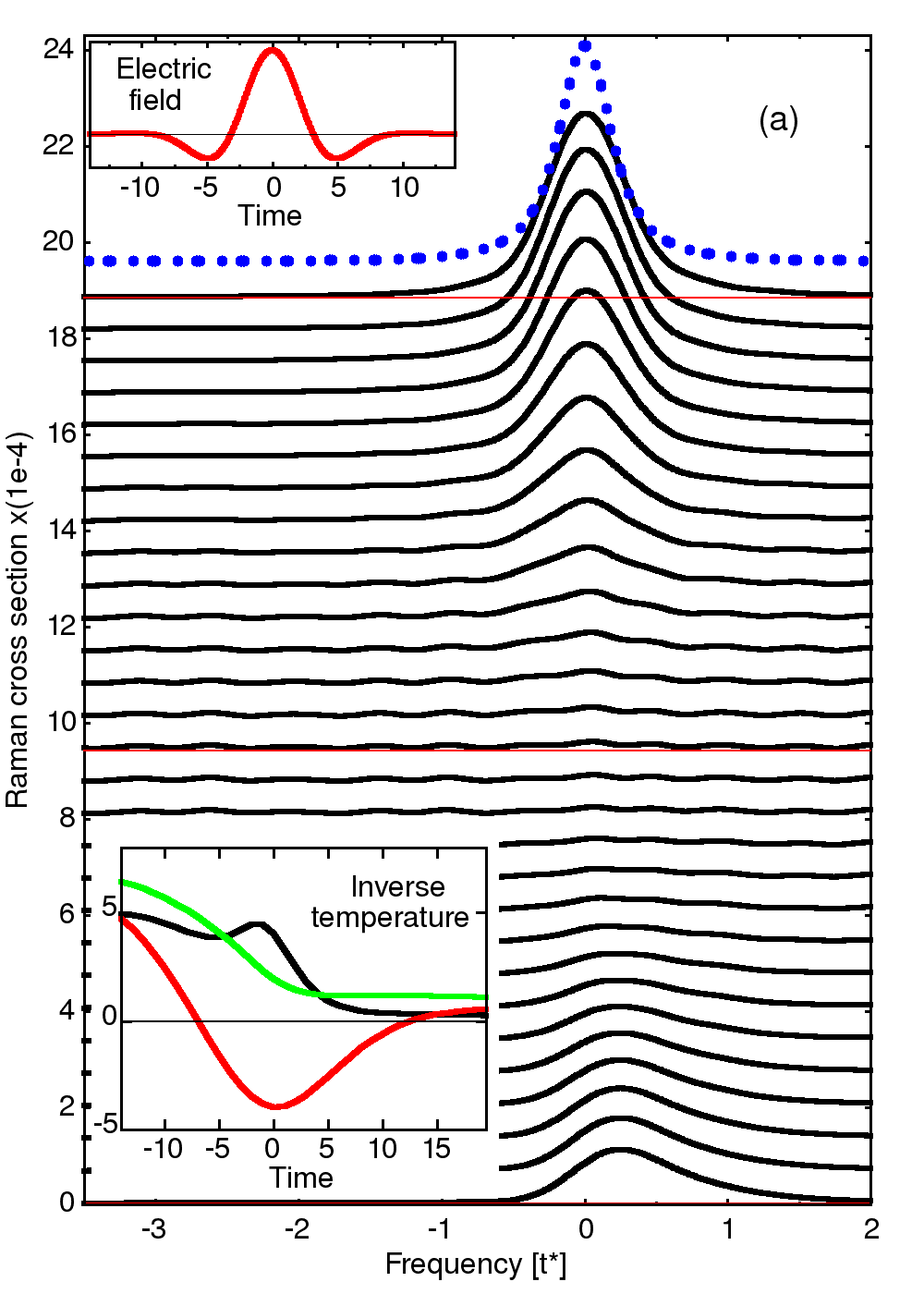
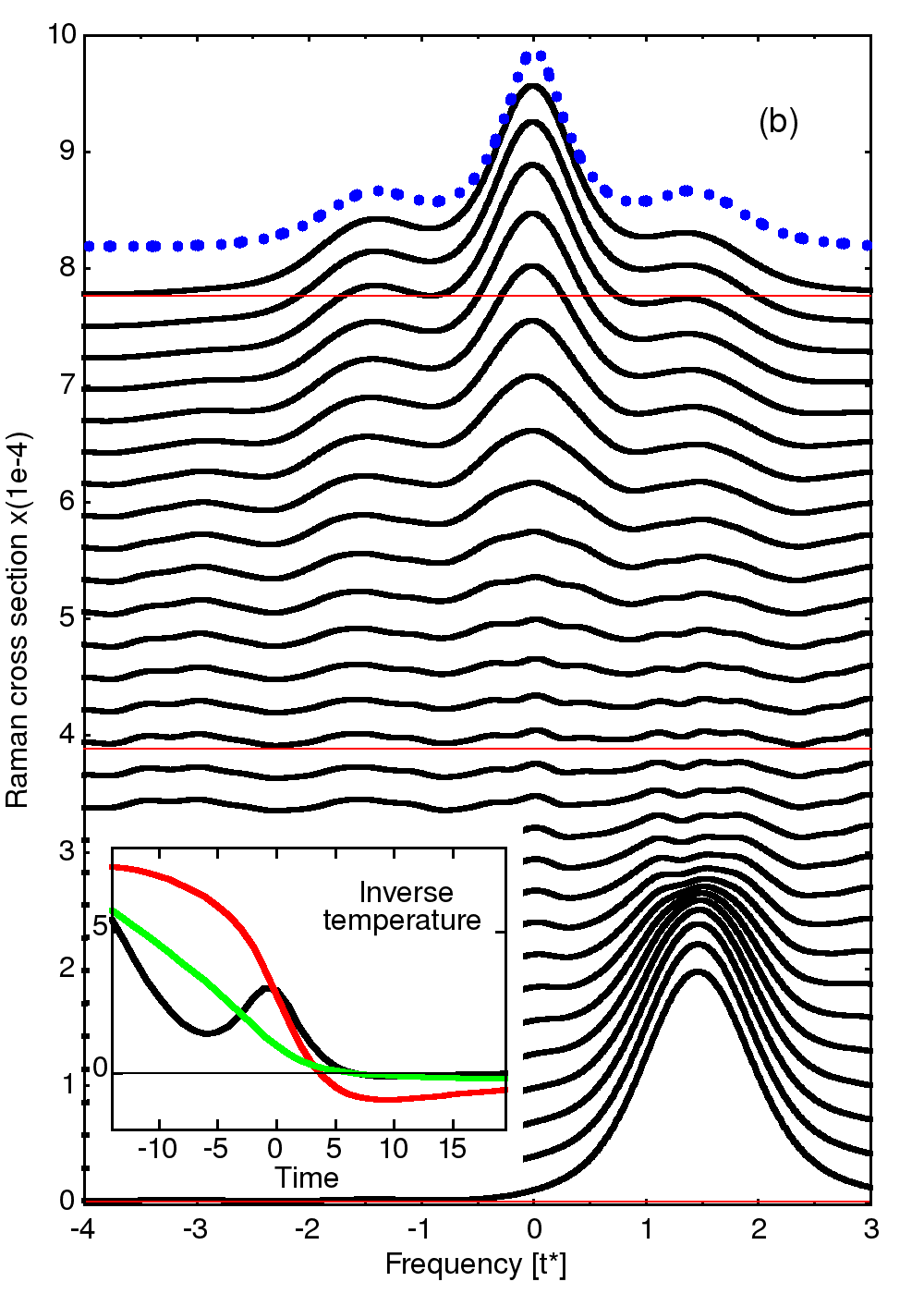
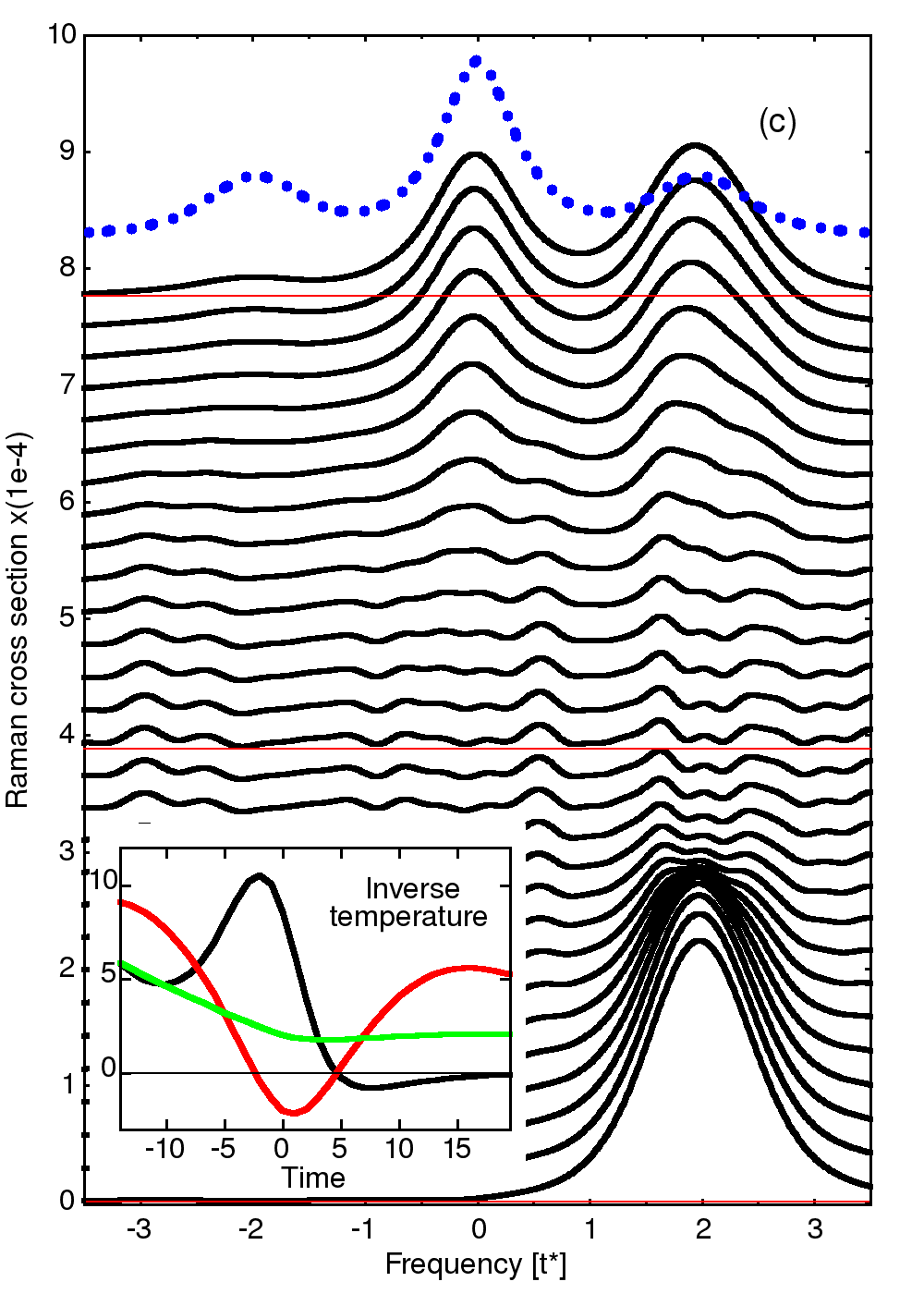
Figure 1: Nonresonant Raman scattering cross section for (a) $U=0.5$, (b) $U=1.5$, and (c) $U=2.0$. Different lines correspond to different time delays $t_{0}\in[-14,14]$ of the probe pulse with respect to the pump one. The pump pulse field is plotted in the upper inset in panel (a) with the following parameters: $\mathbf{E}_{0}=30$, $t_{p}=0$; $\omega_{p}=0.5$, and $\sigma_{p}=5$. The probe pulse width is $\sigma_{b}=12$. The infinite-temperature limit is shown with the blue dotted lines. The lower insets shows the time dependence of the inverse temperature: the black curve is from the Stokes/anti-Stokes ratio; the red curve is from the slope of the single-particle distribution function and the green curve is from a least squares fit to the Fermi-Dirac distribution function; the initial temperature is $T=0.1$ ($\beta=1/T=10$), but the effective temperature only approaches that value for earlier experimental times Shvaika et al. (2018).

We present our results for the nonresonant Raman scattering cross section in Fig. 1: panel (a) is a metal, panel (b) is a near critical Mott-insulator, and panel (c) is a Mott-insulator. For all three cases, we see some common behavior; in equilibrium, the electronic Raman scattering has a broad peak set by the bandwidth for the metal, which evolves into a Mott peak centered at $U$ for the Mott insulator. At early times, there is one peak near $\Omega=U$ (Stokes line) which corresponds to the charge-transfer peak in equilibrium. As the pump is applied $(t_{0}\approx 0)$, it completely suppresses this process due to strong Bloch oscillations of the stress tensor $\gamma_{\alpha\beta}(t)$ Shvaika et al. (2018). After the pump is gone the Raman scattering becomes different for different $U$’s. At late times there is always a peak around $\Omega=0$, which is no longer Pauli blocked due to the excitation of electrons from the pump and comes from hot electrons generated by the pump pulse.

In the insets, we present the time evolution of the effective inverse temperatures $\beta_{\text{eff}}=1/T_{\text{eff}}$ for the single-particle (red and green lines) and two-particle (black line) excitations and one can see that at late times $\beta_{\text{eff}}$ becomes very small. We also plot the $T\to\infty$ equilibrium Raman cross section with the blue dotted line, which is close to the nonequilibrium one at late times. For large $U=2.0$ (Fig. 1(c)) there are two more peaks after the pump is gone: the charge-transfer Stokes and anti-Stokes peaks at $\Omega=\pm U$. In the near-critical Mott-insulator with $U=1.5$ in Fig. 1(b), there are three peaks at late times that correspond to the “zero-peak” and to the restored charge-transfer peaks at $\Omega=U$ (Stokes) and at $\Omega=-U$ (anti-Stokes). Moreover, the anti-Stokes’ peak is higher than the Stokes’ peak, which implies a negative temperature.

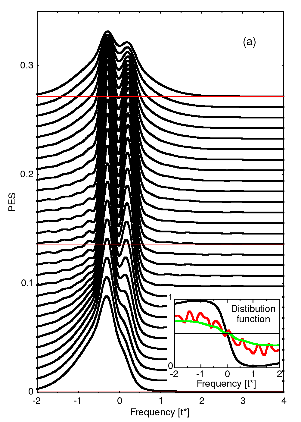
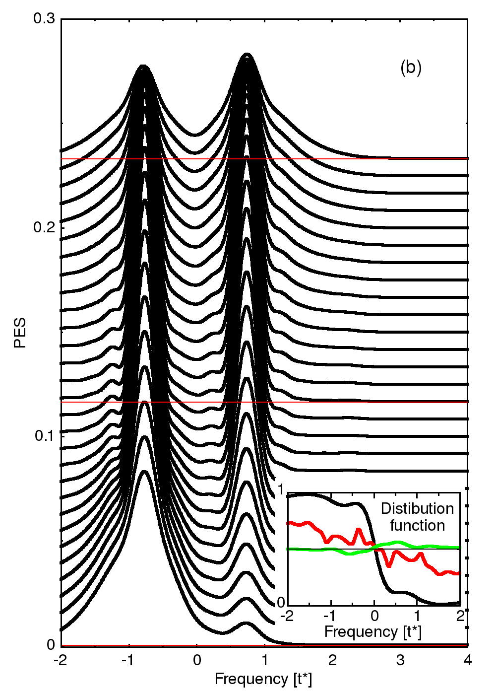
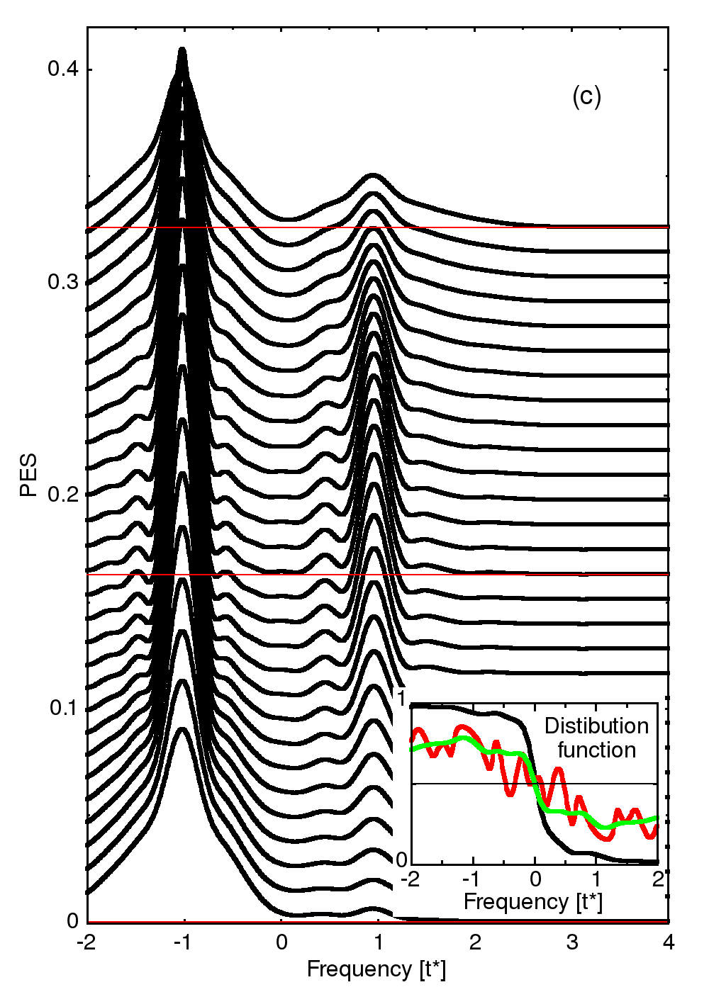
Figure 2: tr-PES: (a), (b), and (c) correspond to $U=0.5$, $U=1.5$, and $U=2.0$. Different lines correspond to different time delays $t_{0}\in[-14,14]$. The inset shows the fermionic distribution function at $t_{0}=-14$ (black), $t_{0}=0$ (red), and $t_{0}=14$ (green).

For comparison, we present our results for the tr-PES in Fig. 2. Similar to the Raman scattering in Fig. 1, the three different panels correspond to different $U$ values, and different curves correspond to different delay times $t_{0}$. In the insets, we show the nonequilibrium distribution function at times $t_{0}=-14$ (black curve), $t_{0}=0$ (red curve), and $t_{0}=14$ (green curve). The pump field excites electrons to the upper band, and after the pump is gone they de-excite back to the lower band in the cases of $U=0.5$ and $U=2.0$ in Fig. 2 (a) and (c), respectively. But in the case of the near-critical Mott-insulator at $U=1.5$ in Fig. 2 (b) it is the opposite: the magnitude of the tr-PES response from the upper band is larger than from the lower one at late times. This means that we observe an inverse occupation of the single-particle electron states characterized by a negative temperature. This is also seen from the plots for the nonequilibrium distribution function: the slope of the green curve which corresponds to late time $t=14$ at zero frequency in Fig. 2 (b) has an opposite sign with respect to other curves on this inset as well as to those in panels (a) and (c).

In the bottom insets in Fig. 1, we show the effective inverse temperature calculated from the Stokes to anti-Stokes ratio in Eq. (8) (black curve) and from the slope of the nonequilibrium distribution function $f_{s}(\omega,t_{0})$ at the Fermi level, which we extracted from the tr-PES results using Eqs. (9) and (Stroboscopic Tests for Thermalization of Electrons in Pump/Probe Experiments) (red curve) and by least squares interpolation of the Fermi-Dirac distribution (green curve). Exploring the behavior of the inverse temperature during the pump, one may speculate on the sensitivity of the single-particle excitations measured by tr-PES and the two-particle excitations measured by Raman scattering to nonequilibrium pumping. The population of the single-particle states is changed very rapidly with the pump for small values of the Coulomb interaction $U=0.5$ and changes very slowly for the large gap Mott insulator at $U=2$, whereas for the near-critical Mott insulator $U=1.5$ the gap is small enough to allow fast population of the upper band but large enough to prevent back de-excitation, leading to an inverse occupation and negative temperatures. At later times the effective temperatures are high leading to the creation of hot electrons as manifested by the flattened electronic distribution function and by the central peak in the Raman cross section. The two-particle excitations are a signature of the creation of bound states, which behave like a heavy subsystem with a different effective temperature and relaxation time than the single-particle one.

Note how the effective temperature of the two-particle excitations initially increases with the pump, but then starts to decrease, reaching its minimum at the pump maximum, after which it starts to increase again. Such behavior can be explained by two effects. First, it is the consequence of a suppression of Raman scattering by Bloch oscillations and, second, the hot electrons destroy the bound states decreasing their density which, together with rapid heating of light single-particle excitations, leads to adiabatic cooling of the heavy (two-particle) subsystem. Of course, because the isolated Falicov-Kimball model does not thermalize, the green and black curves never agree at long times, but they can become close when one is near infinite temperature.

In conclusion, we employed the theory for nonresonant electronic Raman scattering in the $B_{\text{1g}}$ symmetry channel to show how one can measure both fermionic and collective bosonic temperatures stroboscopically in a pump/probe experiment. By comparing these effective temperatures to each other, we can determine how far from equilibrium the electrons are (since these two temperatures must agree in equilibrium). Given the fact that a good fit to a Fermi-Dirac distribution may still involve nonequilibrium electrons, this consistency test across fermions and collective bosonic excitations provides a stringent test for the approach to thermal equilibrium.

Acknowledgments: This work was supported by the Department of Energy, Office of Basic Energy Sciences, Division of Materials Sciences and Engineering under Contract Nos. DE-AC02-76SF00515 (Stanford/SIMES) and DE-FG02-08ER46542 (Georgetown). Computational resources were provided by the National Energy Research Scientific Computing Center supported by the Department of Energy, Office of Science, under Contract No. DE- AC02-05CH11231. J.K.F. was also supported by the McDevitt bequest at Georgetown.

References

- Hsieh et al. (2012) D. Hsieh, F. Mahmood, D. H. Torchinsky, G. Cao, and N. Gedik, “Observation of a metal-to-insulator transition with both Mott-Hubbard and Slater characteristics in Sr2IrO4 from time-resolved photocarrier dynamics,” Phys. Rev. B 86, 035128 (2012).
- Hellmann et al. (2010) S. Hellmann, M. Beye, C. Sohrt, T. Rohwer, F. Sorgenfrei, H. Redlin, M. Kalläne, M. Marczynski-Bühlow, F. Hennies, M. Bauer, A. Föhlisch, L. Kipp, W. Wurth, and K. Rossnagel, “Ultrafast melting of a charge-density wave in the Mott insulator ,” Phys. Rev. Lett. 105, 187401 (2010).
- Perfetti et al. (2006) L. Perfetti, P. A. Loukakos, M. Lisowski, U. Bovensiepen, H. Berger, S. Biermann, P. S. Cornaglia, A. Georges, and M. Wolf, “Time evolution of the electronic structure of through the insulator-metal transition,” Phys. Rev. Lett. 97, 067402 (2006).
- Wegkamp et al. (2014) Daniel Wegkamp, Marc Herzog, Lede Xian, Matteo Gatti, Pierluigi Cudazzo, Christina L. McGahan, Robert E. Marvel, Richard F. Haglund, Angel Rubio, Martin Wolf, and Julia Stähler, “Instantaneous band gap collapse in photoexcited monoclinic due to photocarrier doping,” Phys. Rev. Lett. 113, 216401 (2014).
- Smallwood et al. (2016a) Christopher L. Smallwood, Robert A. Kaindl, and Alessandra Lanzara, “Ultrafast angle-resolved photoemission spectroscopy of quantum materials,” EPL (Europhys. Lett.) 115, 27001 (2016a).
- Giannetti et al. (2016) Claudio Giannetti, Massimo Capone, Daniele Fausti, Michele Fabrizio, Fulvio Parmigiani, and Dragan Mihailovic, “Ultrafast optical spectroscopy of strongly correlated materials and high-temperature superconductors: a non-equilibrium approach,” Adv. Phys. 65, 58–238 (2016).
- Yang et al. (2017) Jhih-An Yang, Stephen Parham, Daniel Dessau, and Dmitry Reznik, “Novel electron-phonon relaxation pathway in graphite revealed by time-resolved Raman scattering and angle-resolved photoemission spectroscopy,” Sci. Rep. 7, 40876 (2017).
- Falicov and Kimball (1969) L. M. Falicov and J. C. Kimball, “Simple model for semiconductor-metal transitions: SmB6 and transition-metal oxides,” Phys. Rev. Lett. 22, 997–999 (1969).
- Freericks et al. (2006) J. K. Freericks, V. M. Turkowski, and V. Zlatić, “Nonequilibrium dynamical mean-field theory,” Phys. Rev. Lett. 97, 266408 (2006).
- Brandt and Mielsch (1989) U. Brandt and C. Mielsch, “Thermodynamics and correlation functions of the Falicov-Kimball model in large dimensions,” Z. Phys. B: Condens. Matter 75, 365–370 (1989).
- Freericks and Zlatić (2003) J. K. Freericks and V. Zlatić, “Exact dynamical mean-field theory of the Falicov-Kimball model,” Rev. Mod. Phys. 75, 1333–1382 (2003).
- Nozières and Abrahams (1974) Philippe Nozières and Elihu Abrahams, “Threshold singularities of the x-ray Raman scattering in metals,” Phys. Rev. B 10, 3099–3112 (1974).
- Shastry and Shraiman (1990) B. Sriram Shastry and Boris I. Shraiman, “Theory of Raman scattering in Mott-Hubbard systems,” Phys. Rev. Lett. 65, 1068–1071 (1990).
- Freericks and Devereaux (2001a) J. K. Freericks and T. P. Devereaux, “Raman scattering through a metal-insulator transition,” Phys. Rev. B 64, 125110 (2001a).
- Shvaika et al. (2004) A. M. Shvaika, O. Vorobyov, J. K. Freericks, and T. P. Devereaux, “Resonant enhancement of inelastic light scattering in strongly correlated materials,” Phys. Rev. Lett. 93, 137402 (2004).
- Shvaika et al. (2005) A. M. Shvaika, O. Vorobyov, J. K. Freericks, and T. P. Devereaux, “Electronic Raman scattering in correlated materials: A treatment of nonresonant, mixed, and resonant scattering using dynamical mean-field theory,” Phys. Rev. B 71, 045120 (2005).
- Devereaux and Hackl (2007) Thomas P. Devereaux and Rudi Hackl, “Inelastic light scattering from correlated electrons,” Rev. Mod. Phys. 79, 175–233 (2007).
- Kadanoff and Baym (1962) L. P. Kadanoff and G. Baym, Quantum Statistical Mechanics (W. A. Benjamin, Inc., New York, 1962).
- Keldysh (1965) L. V. Keldysh, “Diagram technique for nonequilibriun processes,” Sov. Phys. JETP 20, 1018–1026 (1965).
- Zlatic and Horvatic (1990) V. Zlatic and B. Horvatic, “The local approximation for correlated systems on high dimensional lattices,” Solid State Commun. 75, 263–267 (1990).
- Freericks and Devereaux (2001b) J. K. Freericks and T. P. Devereaux, “Non-resonant Raman scattering through a metal-insulator transition: An exact analysis of the Falicov-Kimball model,” Condens. Matter Phys. 4, 149–160 (2001b).
- Shvaika et al. (2018) A. M. Shvaika, O. P. Matveev, T. P. Devereaux, and J. K. Freericks, “Interpreting pulse-shape effects in pump-probe spectroscopies,” Condens. Matter Phys. 21, 33707 (2018), arXiv:1808.04983 .
- Freericks et al. (2009) J. K. Freericks, H. R. Krishnamurthy, and Th. Pruschke, “Theoretical description of time-resolved photoemission spectroscopy: Application to pump-probe experiments,” Phys. Rev. Lett. 102, 136401 (2009).
- Smallwood et al. (2016b) Christopher L. Smallwood, Tristan L. Miller, Wentao Zhang, Robert A. Kaindl, and Alessandra Lanzara, “Nonequilibrium electron dynamics in a solid with a changing nodal excitation gap,” Phys. Rev. B 93, 235107 (2016b).
- Stafford (2016) Charles A. Stafford, “Local temperature of an interacting quantum system far from equilibrium,” Phys. Rev. B 93, 245403 (2016).