Thermodynamic calculation of spin scaling functions

Abstract

Critical phenomena theory centers on the scaled thermodynamic potential per spin $\phi(\beta,h)=|t|^{p}Y(h|t|^{-q})$, with inverse temperature $\beta=1/T$, $h=-\beta H$, ordering field $H$, reduced temperature $t=t(\beta)$, critical exponents $p$ and $q$, and function $Y(z)$ of $z=h|t|^{-q}$. I discuss calculating $Y(z)$ with the information geometry of thermodynamics. Scaled solutions obtain with three admissible functions $t(\beta)$: 1) $t=e^{-J\beta}$, 2) $t=\beta^{-1}$, and 3) $t=\beta_{C}-\beta$, where $J$ and $\beta_{C}$ are constants. For $p=q$, information geometry yields $Y(z)=\sqrt{1+z^{2}}$, consistent with the one-dimensional (1D) ferromagnetic Ising model.

Keywords: Information geometry of thermodynamics; Scaled equation of state; Ising model; Spherical model; Thermodynamic curvature; Phase transitions and critical points.

Critical point theory deals with systems with long-range order, measured by a diverging correlation length $\xi$ [1, 2]. Here, it is hard to evaluate the partition function $Z$ by summing over microstates. In this letter, I approach the problem of long-range order with a method not based on an explicit summation over microstates. I combine the curvature scalar $R$ from the information geometry of thermodynamics with hyperscaling, to get a differential equation for the thermodynamics.

1 Introduction

I employ the language of magnetic systems, for which the thermodynamic potential per spin is $\phi=\phi(\beta,h)$, where $\beta=1/T$, with $T$ the temperature, and $h=-\beta H$, with $H$ the ordering field. Boltzmann’s constant $k_{B}=1$. In the language of Pathria and Beale [2], $\phi$ is the $q$-potential per spin: $\phi(\beta,h)=\mbox{ln}Z/N$, and $N$ is the number of spins $(N\to\infty)$. The heat capacity per spin at constant $H$ is $C_{H}=T(\partial s/\partial T)_{H}$, with entropy per spin $s=\phi-\beta\phi_{,\beta}-h\phi_{,h}$. The magnetic susceptibility is $\chi_{T}=(\partial m/\partial H)_{T}$, with magnetization per spin $m=-\phi_{,h}$. The comma notation denotes differentiation.

Critical phenomena theory centers on scaling and universality, expressed by a scaled relation:

$$\phi(\beta,h)=n_{1}|t|^{p}\,Y(n_{2}\,h|t|^{-q}),$$ (1)

where $p$ and $q$ are critical exponents, $t=t(\beta)$ is the reduced temperature, $n_{1}$ and $n_{2}$ are scaling constants, and $Y(z)$ is a universal function of

$$z=h|t|^{-q}.$$ (2)

I consider critical points both at a finite critical temperature $T_{C}$, and at zero temperature.

As I will show explicitly, the information geometric method allows three admissible functions leading to scaled solutions for $t=t(\beta)$:

$$1)\,t=e^{-J\beta},2)\,t=\beta^{-1},\mbox{ and }3)\,t=\beta_{C}-\beta,$$ (3)

where $J$ is a constant and $\beta_{C}=1/T_{C}$. These three admissible functions for $t=t(\beta)$ are familiar from the modern theory of critical phenomena. Figure 1 sketches the corresponding critical point scenarios. The function 3) was identified previously as admissible in the information geometric approach [3]. The contribution in this letter is the identification of the exponential function 1) and the power law function 2) as admissible as well. These two functional forms are characteristic of critical points at zero temperature.

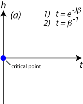
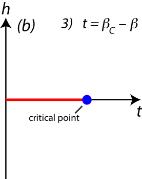
Figure 1: The critical region in $(t,h)$ space: a) critical temperature $T_{C}=0$, with no first-order phase transition line, and b) $T_{C}>0$, with a first-order phase transition line shown in red.

The information geometric method allows for the determination of $Y(z)$, based on the character of the critical point, and the values of the critical exponents. This is difficult to accomplish with statistical mechanics, and very few cases have been worked out.

2 The 1D Ising model

A worked example is the one-dimensional (1D) ferromagnetic Ising model consisting of a chain of $N$ spins ($N\to\infty$) enumerated by an index $i$. The $i$’th spin has state $\sigma_{i}=+1/-1$, corresponding to spin up/down. The Hamiltonian is

$$\mathcal{H}=-J\sum_{i=1}^{N}\sigma_{i}\sigma_{i+1}-H\sum_{i=1}^{N}\sigma_{i},$$ (4)

where $J>0$ is the coupling constant, and we assume periodic boundary conditions: $\sigma_{N+1}=\sigma_{1}$.

Evaluating the partition function with statistical mechanics leads to [2]:

$$\phi(\beta,h)=\mbox{ln}\left(e^{J\beta}\cosh h+\sqrt{e^{2J\beta}\,\mbox{sinh}^{2}h+e^{-2J\beta}}\,\right),$$ (5)

yielding a critical point at $h=0$ and $T=0$, where $\chi_{T}$ and $\lvert R\rvert$ diverge. Nelson and Fisher [4] worked out the scaled form for the singular part of Eq. (5) near the critical point:

$$\phi=e^{-2J\beta}\,Y(h\,e^{2J\beta}),$$ (6)

with

$$z=h\,e^{2J\beta},$$ (7)

and

$$Y(z)=\sqrt{1+z^{2}}.$$ (8)

These authors took $t(\beta)=e^{-J\beta}$, and $p=q=2$.

The critical exponents of this model are ambiguous since a dimensionless factor may be removed from $J$ in $t=e^{-J\beta}$, and put into $p$ and $q$. But this will pose no difficulties for the information geometric method since all exponent choices lead to the same scaled equation of state if $p=q$.

3 Information geometry of thermodynamics

Strong features of the information geometric calculation method are: 1) the scaled universal function in Eq. (1) fits naturally into the structure, 2) $Y(z)$ may be calculated by solving an ordinary differential equation, and 3) strong constraints are put on appropriate choices for $t=t(\beta)$. We also have a special result for the case $p=q$, a case that includes the 1D ferromagnetic Ising model.

Essential in information geometry is the invariant thermodynamic curvature $R$, resulting from the thermodynamic metric elements $g_{\alpha\beta}=\phi_{,\alpha\beta}$ [5]. Here, the thermodynamic coordinates are $(x^{1},x^{2})=(\beta,h)$. For spin systems, $R$ has units of lattice constants to the power of the spatial dimension [6]. For weakly interacting systems, $\lvert R\rvert$ is small, and on approaching a critical point, $R$ diverges to negative infinity. Here, I use the sign convention of Weinberg [7], where the curvature of the two-sphere is negative.

It has long been argued [5, 8, 9] that near a critical point

$$\lvert R\rvert\propto\xi^{d},$$ (9)

where $d$ is the spatial dimension. In addition, hyperscaling from the theory of critical phenomena has [10, 11]:

$$\lvert\phi\rvert\propto\xi^{-d}.$$ (10)

Eliminating $\xi^{d}$ between these two proportionalities leads to

$$R=-\frac{\kappa}{\phi},$$ (11)

where $\kappa$ is a dimensionless constant of order unity that the solution method determines. The known expression of $R$ for spin systems allows us to write Eq. (11) as [5]

$$\phi\left|\begin{array}[]{ccc}\phi_{,11}&\phi_{,12}&\phi_{,22}\\ \phi_{,111}&\phi_{,112}&\phi_{,122}\\ \phi_{,112}&\phi_{,122}&\phi_{,222}\end{array}\right|\displaystyle=-2\kappa\left|\begin{array}[]{cc}\phi_{,11}&\phi_{,12}\\ \phi_{,12}&\phi_{,22}\end{array}\right|^{2}.$$ (12)

This geometric equation is a third-order partial differential equation (PDE) for $\phi$. It is written in terms of the macroscopic thermodynamic parameters, with its mesoscopic roots entirely hidden. Although the argument above for this equation is somewhat loose, I conjecture that Eq. (12) is exact near the critical point. This equation has seen success in varied scenarios, not all connected with critical phenomena; see Table 1.

Table 1: Tests of the geometric equation. $n$ denotes the number of independent thermodynamic variables, $d$ the spatial dimension, $a\#$ the number of analytic sections, and $f$ the number of fit parameters for the scaled equation.

System	$n$	$d$	$a\#$	$f$	notes
mean field theory [12]	$2$	$-$	$1$	$0$	exact
critical point [12]	$2$	$3$	$2$	$2$	$\chi^{2}\sim 1$
galaxy clustering [13]	$2$	$3$	$1$	$0$	qualitative
corrections to scaling [3]	$3$	$3$	$2$	$3$	unclear
ideal gas paramagnet [14]	$3$	$3$	$1$	$0$	exact
power law interacting fluids [15]	$2$	$3$	$1$	$1$	qualitative
unitary fermi fluid [16, 17]	$2$	$3$	$2$	$4$	$\chi^{2}\sim 2$
black holes [18]	$2$	$-$	$1$	$1$	unclear
ferromagnetic Ising	$2$	$1$	$1$	$0$	exact

4 Results

For each of the three functions for $t(\beta)$ in Eq. (3), the PDE Eq. (12) simplifies to a third-order ordinary differential equation (ODE) for $Y(z)$ on substituting the scaled expression in Eq. (1) for $\phi$. To see the reason for this reduction in complexity, imagine expanding out the two determinants in Eq. (12). The result is an equation consisting of nine terms. Each term contains a quadruple of four factors of $\phi$, four derivatives with respect to $\beta$, and four derivatives with respect to $h$. For each of the three functional forms in Eq. (3), differentiating $\phi$ or its derivatives with respect to $\beta$ or with respect to $h$ pulls out a factor of a power of $t(\beta)$. These common factors in the quadruples all cancel out, leaving only $z$, $Y(z)$, and its derivatives. I found no other functions $t(\beta)$ that result in this cancellation of factors of $t(\beta)$.

Including the scaling constants $n_{1}$ and $n_{2}$ in $\phi$, as in Eq. (1), likewise results in a cancellation of all factors $n_{1}$ and $n_{2}$. The same ODE, with the same solution $Y(z)$, results. The ODE and $Y(z)$ generally depend only on the critical exponents $p$ and $q$. This dependence is expected from the theory of critical phenomena, where changing the critical exponents put us into a different universality class, with different $Y(z)$’s.

Consider now in detail the solution with the exponential form for $t(\beta)$:

$$\phi=\exp(-pJ\beta)\,Y(h\exp[qJ\beta]).$$ (13)

This form has not been previously considered in the context of information geometry. Particularly simple is the case $q=p$, of which the 1D ferromagnetic Ising model is an example. For $q=p$, Eq. (12) simplifies to

$$\frac{Y\left(zYY^{(3)}+z^{2}Y^{\prime\prime 2}+2YY^{\prime\prime}-z^{2}Y^{\prime}Y^{(3)}-2zY^{\prime}Y^{\prime\prime}\right)}{2\left(Y-zY^{\prime}\right)^{2}Y^{\prime\prime}}=\kappa,$$ (14)

independent of the value of $p$. The cancellation of $p$ is physically necessary because we may pull any factor out of $J$ and put it into $p$ without changing the physics, as I remarked in connection with the Ising model. More generally, I add that for models with $t=\exp(-J\beta)$ and $q=np$, with $n$ a constant factor, $p$ cancels out as well, leaving $Y(z)$ depending only on $n$.

To solve Eq. (14), start by assuming that $Y(z)$ is analytic at $z=0$, an assumption generally made in theories of critical phenomena for $\beta<\beta_{C}$ [19], and certainly the case in Eq. (8). Also assume that $Y(z)$ is symmetric about $z=0$, a general feature of the basic Ising spin models. We have the series

$$Y(z)=y_{0}+y_{2}z^{2}+y_{4}z^{4}+\cdots,$$ (15)

where $y_{0}$, $y_{2}$, $y_{4}\cdots$ are constant coefficients. Substituting this series into Eq. (14) yields

$$1+\left(\frac{3y_{2}}{y_{0}}+\frac{6y_{4}}{y_{2}}\right)z^{2}+\left(\frac{5y_{2}^{2}}{y_{0}^{2}}+\frac{22y_{4}}{y_{0}}-\frac{36y_{4}^{2}}{y_{2}^{2}}+\frac{30y_{6}}{y_{2}}\right)z^{4}+\cdots=\kappa.$$ (16)

Clearly, we must have $\kappa=1$, a value independent of the series coefficients. The series constants $y_{0}$ and $y_{2}$ may assume any values consistent with thermodynamic stability, but $y_{4}$, $y_{6}\cdots$ are determined by equating each coefficient on the left-hand side second-order and higher to zero, leading to $y_{4}=-\frac{1}{2}y_{2}^{2}/y_{0}$, etc. The coefficients $y_{0}$ and $y_{2}$ are two of the integration constants. The third is the first-order series coefficient $y_{1}$ that was set to zero in Eq. (15). Setting $y_{1}=0$ results in all the odd-order series coefficients to be zero.

The resulting series solution corresponds to the function:

$$Y(z)=n_{1}\sqrt{1+(n_{2}z)^{2}},$$ (17)

where the scaling constants $n_{1}$ and $n_{2}$ are simply related to $y_{0}$ and $y_{2}$. Direct substitution of this function into Eq. (14) demonstrates that it is indeed the even solution analytic at $z=0$. This solution matches exactly what is known for the 1D Ising model in Eq. (8) with $n_{1}=n_{2}=1$. This finding is the main result in this letter. An additional finding is that with $q=p$ all three of the reduced temperature expressions $t({\beta})$ in Eq. (3) lead to the same ODE. Assuming even solutions analytic at $z=0$, all the $q=p$ cases have the solution Eq. (17).

A calculation with statistical mechanics of the scaling function $Y(z)$ in a magnetic field is usually very difficult. I am not aware of other simple worked examples not already on the list in Table 1. It is my hope that the considerations in this letter will spur such calculations.

One possible candidate for further investigation is the spherical model [2, 20], which has instances of $t(\beta)$ of the power law varieties, $2)$ and $3)$ in Eq. (3). The spherical model was originally devised as a solvable spin model. In integer dimension $d$, it is a generalization of the Ising model. In continuous dimension $0<d<2$, it has critical point at $T_{C}=0$, and it has $t(\beta)=\beta^{-1}$. Baker and Bonner [21] reported:

$$\phi=\beta^{-p}\,Y\left(h\beta^{p}\right),$$ (18)

with $p=d/(2-d)$, though no specific functional form for $Y(z)$ was given. We have $q=p$, and if we assume that $Y(z)$ is an even function analytic at $z=0$, we get the scaled form $Y(z)=\sqrt{1+z^{2}}$, as in Eq. (17).

The spherical model with $d>2$ has a critical point at nonzero temperature [2]. Janke et al. [22] discussed this case in the context of calculating $R$, and stated that $t(\beta)=\beta_{C}-\beta$, putting it into category 3) in Eq. (3). But no $Y(z)$ was reported.

5 Conclusion

In conclusion, I have extended an information geometric method for calculating scaling functions to cases involving spin systems. I focused on the 1D ferromagnetic Ising model, and showed that the method produces the correct scaling function. Calculations of the scaling functions with information geometry are straightforward; they involve solving differential equations. Calculations with statistical mechanics in models are considerably harder, and there very few known cases in field. The challenge is to produce more.

References

- [1] Stanley, H.E., “Scaling, universality, and renormalization: Three pillars of modern critical phenomena,” Rev. Mod. Phys. 71, S358 (1999).
- [2] Pathria, R. K., and Beale, P. D., Statistical Mechanics (Butterworth-Heinemann, Oxford, UK, 2011).
- [3] Ruppeiner, G., “Riemannian geometric approach to critical points: General theory,” Phys. Rev. E 57, 5135 (1998).
- [4] Nelson, D. R., and Fisher, M. E., “Soluble Renormalization Groups and Scaling Fields for Low-Dimensional Ising Systems,” Annals of Physics 91, 226 (1975).
- [5] Ruppeiner, G., “Riemannian geometry in thermodynamic fluctuation theory,” Rev. Mod. Phys. 67, 605 (1995); 68, 313(E) (1996).
- [6] Ruppeiner, G., and Bellucci, S., “Thermodynamic curvature for a two-parameter spin model with frustration,” Phys. Rev. E 91, 012116 (2015).
- [7] Weinberg, S., Gravitation and Cosmology (Wiley, New York, NY, USA, 1972).
- [8] Ruppeiner, G., “Thermodynamics: A Riemannian geometric model,” Phys. Rev. A 20, 1608 (1979).
- [9] Johnston, D. A., Janke, W., and Kenna, R., “Information geometry, one, two, three (and four),” Acta Phys. Pol. B 34, 4923 (2003).
- [10] Widom, B., “The critical point and scaling theory,” Physica 73, 107 (1974).
- [11] Goodstein, D. L., States of Matter (Prentice-Hall, Englewood Cliffs, NJ, 1975).
- [12] Ruppeiner, G., “Riemannian geometric theory of critical phenomena,” Phys. Rev. A 44, 3583 (1991).
- [13] Ruppeiner, G., “Equations of state of large gravitating gas clouds,” Astrophys. J. 464, 547 (1996).
- [14] Kaviani, K., and Dalafi-Rezaie, A., “Pauli paramagnetic gas in the framework of Riemannian geometry,” Phys. Rev. E 60, 3520 (1999).
- [15] Ruppeiner, G., “Riemannian geometry of thermodynamics and systems with repulsive power-law interactions,” Phys. Rev. E 72, 016120 (2005).
- [16] Ruppeiner, G., “Unitary Thermodynamics from Thermodynamic Geometry,” J. Low Temp. Phys. 174, 13 (2014).
- [17] Ruppeiner, G., “Unitary Thermodynamics from Thermodynamic Geometry II: Fit to a Local-Density Approximation,” J. Low Temp. Phys. 181, 77 (2015).
- [18] Ruppeiner, G., “Thermodynamic black holes,” Entropy 20, 460 (2018).
- [19] Griffiths, R. B., “Thermodynamic Functions for Fluids and Ferromagnets near the Critical Point,” Phys. Rev. 158, 176 (1967).
- [20] Berlin, T. H., and Kac, M., “The Spherical Model of a Ferromagnet,” Phys. Rev. 86, 821 (1952).
- [21] Baker, G. A., and Bonner, J. C., “Scaling behavior at zero-temperature critical points,” Phys. Rev. B 12, 3741 (1975).
- [22] Janke, W., Johnston, D. A., and Kenna, R., “Information geometry of the spherical model,” Phys. Rev. E 67, 046106 (2003).