Natural Stabilization of the
Higgs Boson’s Mass and Alignment

Abstract

Current data from the LHC indicate that the $125\,{\rm GeV}$ Higgs boson, $H$, is either the single Higgs of the Standard Model or, to a good approximation, an “aligned Higgs”. We propose that $H$ is the pseudo-Goldstone dilaton of Gildener and Weinberg. Models based on their mechanism of scale symmetry breaking can naturally account for the Higgs boson’s low mass and aligned couplings. We conjecture that they are the only way to achieve a “Higgslike dilaton” that is actually the Higgs boson. These models further imply the existence of additional Higgs bosons in the vicinity of 200 to about $550\,{\rm GeV}$. We illustrate our proposal in a version of the two-Higgs-doublet model of Lee and Pilaftsis. Our version of this model is consistent with published precision electroweak and collider physics data. We describe tests to confirm, or exclude, this model at Run 3 of the LHC.

1. The Gildener-Weinberg mechanism for
stabilizing the Higgs mass and alignment

The $125\,{\rm GeV}$ Higgs boson $H$ discovered at the LHC in 2012 is a puzzle [1, 2]. Its known couplings to electroweak (EW) gauge bosons ($W$, $Z$, $\gamma$), to gluons and to fermions ($\tau$, $b$ and $t$, so far) are consistent at the 10–20% level with those predicted for the single Higgs of the Standard Model (SM) [3, 4, 5, 6]. But is that all? Why is the Higgs so light — especially in the absence of a shred of evidence for any new physics that could explain its low mass? Is naturalness a chimera?

If there are more Higgs bosons — as favored in most of the new physics proposed to account for $H$ and a prime search topic of the ATLAS and CMS Collaborations — why are $H$’s known couplings so SM-like? The common and attractive answer is that of Higgs alignment. In the context, e.g., of a model with several Higgs doublets,

$$\Phi_{i}=\frac{1}{\sqrt{2}}\left(\begin{array}[]{c}\sqrt{2}\phi_{i}^{+}\\ v_{i}+\rho_{i}+ia_{i}\end{array}\right),\quad i=1,2,\dots,$$ (1)

where $v_{i}/\sqrt{2}$ is the vacuum expectation value (vev) of $\Phi_{i}$, an aligned Higgs is one that is a mass eigenstate given by

$$H=\sum_{i}v_{i}\rho_{i}/v$$ (2)

with $v=\sqrt{\sum_{i}v_{i}^{2}}=246\,{\rm GeV}$. Eq. (2) has the same form as the linear combination of $\phi^{\pm}_{i}$ and $a_{i}$ eaten by the $W^{\pm}$ and $Z$. And this $H$ has exactly SM couplings to $W$, $Z$, $\gamma$, gluons and the quarks and leptons.

To our knowledge, the first discussion of an aligned Higgs boson appeared in Ref. [7]. It was discussed there in the context of a two-Higgs-doublet model (2HDM) in the “decoupling limit” in which all the particles of one doublet are very much heavier than $v$, and so decouple from EW symmetry breaking. The physical scalar of the lighter doublet then has SM couplings.

There have been many papers on Higgs alignment in the literature since Ref. [7], including others not assuming the decoupling limit; see, e.g., Ref. [8]. However, with only a few exceptions, see Refs. [9, 10, 11, 12], it appears that they have not addressed an important theoretical question: is Higgs alignment natural? Is there an approximate symmetry which protects it from large radiative corrections? As in these references, this might seem a separate question of naturalness than the radiative stability of the Higgs mass, $M_{H}$. In fact, this question was settled long ago: a single symmetry, spontaneously broken scale invariance with weak explicit breaking, accounts for the Higgs boson’s mass and its alignment.

In 1973, S. Coleman and E. Weinberg (CW) [13] considered a classically scale-invariant theory of a dilaton scalar with an abelian gauge interaction, massless scalar electrodynamics. They showed that one-loop quantum corrections can fundamentally change the character of the theory by explicitly breaking the scale invariance, giving the dilaton a mass and a vev and, thereby, spontaneously breaking the gauge symmetry.

In 1976, E. Gildener and S. Weinberg (GW) [14] generalized CW to arbitrary gauge interactions with arbitrary scalar multiplets and fermions, using a formalism previously invented by S. Weinberg [15]. Despite the generality, their motivation was clearly in the context of what is now known as the Standard Model. They assumed that, due to some unknown, unspecified underlying dynamics, the scalars $\Phi_{i}$ in their model have no mass terms nor cubic couplings and, so, the model is classically scale-invariant.^, The quartic potential of the massless scalar fields, which are real in this notation, is (see Ref. [14] for details)

$$V_{0}(\Phi)=\frac{1}{24}f_{ijkl}\,\Phi_{i}\Phi_{j}\Phi_{k}\Phi_{l},$$ (3)

with dimensionless quartic couplings $f_{ijkl}$. A minimum of $V_{0}$ may or may not spontaneously break any continuous symmetries. If it does, it will also break the scale invariance resulting in a massless Goldstone boson, the dilaton. A minimum of $V_{0}$ does occur for the trivial vacuum, $\Phi_{i}=0$ for all $i$. At this minimum, all fields are massless and scale invariance is realized in the Wigner mode. However, GW supposed that $V_{0}$ has a nontrivial minimum on the ray

$$(\Phi_{n})_{i}=n_{i}\phi,\qquad i=1,2,\dots$$ (4)

where $\sum_{i}n_{i}^{2}=1$ and $\phi>0$ is an arbitrary mass scale. They did this by adjusting the renormalization scale to have a value $\Lambda_{W}$ so that the minimum of the real continuous function $V_{0}(N)$ is zero on the unit sphere $N_{i}N_{i}=1$. If this minimum is attained for a specific unit vector $N_{i}=n_{i}$, then $V_{0}(\Phi)$ has this minimum value everywhere on the ray (4):

$$V_{0}(\Phi=\Phi_{n}\equiv n\phi)=\frac{1}{24}f_{ijkl}\,n_{i}n_{j}n_{k}n_{l}\,\phi^{4}=0.$$ (5)

Obviously, for this to be a minimum,

$$\left.\frac{\partial V_{0}(\Phi)}{\partial\Phi_{i}}\right|_{\Phi_{n}}=f_{ijkl}\,n_{j}n_{k}n_{l}\,\phi^{3}=0,$$ (6)

and the matrix

$$P_{ij}=\textstyle{\frac{1}{2}}f_{ijkl}\,n_{k}n_{l}$$ (7)

must be positive semi-definite.

Now comes the punchline: The combination $\Phi_{n}=n\phi$ is an eigenvector of $P$ with eigenvalue zero. It is the dilaton associated with the ray (4), the flat direction of $V_{0}$’s minimum and the spontaneous breaking of scale-invariance. GW called the Higgs boson $\Phi_{n}$ the “scalon”. Massive eigenstates of $P$ are other Higgs bosons. Any other massless scalars have to be Goldstone bosons ultimately absorbed via the Higgs mechanism. Then, à la CW, one-loop quantum corrections $V_{1}(\Phi)$ can explicitly break the scale invariance, picking out a definite value $\langle\phi\rangle_{0}=v$ of $\phi$ at which $V_{0}+V_{1}$ has a minimum and giving the scalon a mass. Including quantum fluctuations about this minimum,

$$(\Phi_{n})_{i}=n_{i}(v+H)+H^{\prime}_{i}=v_{i}+v_{i}H/v+H^{\prime}_{i},$$ (8)

where, with knowledge aforethought, we name the scalon $H$. The other Higgs bosons $H^{\prime}_{i}$ are orthogonal to $H$. To the extent that $V_{1}$ is not a large perturbation on the masses and mixings of the other Higgs bosons of the tree approximation, the $H_{i}^{\prime}$ are small components of $\Phi_{n}$. Thus, the scalon is an aligned Higgs boson. Furthermore, the alignment of $H$ is protected from large renormalizations in the same way that its mass is: by perturbatively small loop corrections to $V_{0}$ and its scale invariance. While the Higgs’s alignment is apparent in the model we adopt in Sec. 2 as a concrete example [17], this fact and its protected status are not stressed in that paper nor even recognized in any other paper on Higgs alignment we have seen.

From now on, we identify $H$ with the 125 GeV Higgs boson discovered at the LHC. From the one-loop potential, i.e., first-order perturbation theory, GW obtained the following formula for $M_{H}$ (which we restate in the context of known elementary particles, extra Higgs scalars, and their electroweak interactions):

$$M_{H}^{2}=\frac{1}{8\pi^{2}v^{2}}\left(6M_{W}^{4}+3M_{Z}^{4}+\sum_{{\cal H}}M_{{\cal H}}^{4}-12m_{t}^{4}\right).$$ (9)

Here, the sum is over Higgs bosons ${\cal H}$ other than $H$ that may exist. Because this is first-order perturbation theory, the masses on the right side are those determined in zeroth order but evaluated at the scale-invariance breaking value $v$ of $\phi$. For $M_{H}=125\,{\rm GeV}$, Eq. (9) implies the sum rule

$$\left(\sum_{{\cal H}}M_{{\cal H}}^{4}\right)^{1/4}=540\,{\rm GeV}.$$ (10)

This result was obtained in Ref. [18] and used in Ref. [17] to constrain the masses of new scalars. It does not appear to have received the attention it deserves. It applies to all extra-Higgs models based on the GW mechanism that do not contain additional weak bosons or heavy fermions. Thus, the more Higgs multiplets a scalon model has, the lighter they will be. So long as loop factors suppress the higher-order corrections to Eq. (10), it should be a good indication of the mass range of additional Higgs bosons in this very broad class of models.

There have been a number papers on scale invariance leading to a “Higgslike dilaton” before and since the 2012 discovery of the Higgs boson, Refs. [19, 20, 21, 22, 23, 24] to cite several. An especially thorough discussion is contained in Ref. [20]. The authors of this paper examined the possibility that $H(125)$ “actually corresponds to a dilaton: the Goldstone boson of scale invariance spontaneously broken at a scale $f$.” Such a dilaton ($\sigma$) has couplings to EW gauge bosons $W,Z$ and fermions $\psi$ induced by its coupling to the trace of the energy-momentum tensor. They are

$$\left(2gM_{W}W_{\mu}^{+}W^{\mu\,-}+\sqrt{g^{2}+g^{\prime\,2}}M_{Z}Z_{\mu}Z^{\mu}\right)\frac{\sigma v}{f}-\sum_{\psi}\frac{Y_{\psi}}{2}\bar{\psi}_{L}\psi_{R}\left(1+\gamma_{L}+\gamma_{R}\right)\frac{\sigma v}{f}+{\rm h.c.},$$ (11)

where $\gamma_{L,R}$ are possible anomalous dimensions. Apart from $\gamma_{L,R}$, these couplings are the same as those of an SM Higgs, but scaled by $v/f$.

In general, the decay constant of a Higgslike dilaton satisfies $|v/f|\leq 1$. Ref. [20], written about six months after the discovery of $H(125)$, concluded that $|v/f|\mathrel{\hbox to0.0pt{\raise 2.20013pt\hbox{$>$}\hss}{\lower 2.20013pt\hbox{$\sim$}}}0.90$ (assuming that $\gamma_{L,R}=0$). Obviously, the constraint on $|v/f|$ is tighter now, possibly $|v/f|\mathrel{\hbox to0.0pt{\raise 2.20013pt\hbox{$>$}\hss}{\lower 2.20013pt\hbox{$\sim$}}}0.95$, since all measured Higgs signal strengths, ($\sigma(H)B(H\to X))/(\sigma(H)B(H\to X))_{\rm SM}$, would be proportional to $(v/f)^{2}$. An important point stressed by the authors is that $f\simeq v$ (probably $f=v$) is achieved in models in which only operators charged under the EW gauge group obtain vacuum expectation values, i.e., $f=v$ only if the agent responsible for electroweak symmetry breaking (EWSB) is also the one responsible for scale symmetry breaking.

A major obstacle to the Higgslike dilaton stressed in Ref. [20] is that, in non-supersymmetric models it is generally very unnatural that the dilaton’s mass $M_{\sigma}$ is much less than the scale $\Lambda_{f}\simeq 4\pi f$ of the dynamics underlying spontaneous scale symmetry breaking. The authors do mention that a potential of Coleman-Weinberg type (and, by extension, Gildener-Weinberg) can naturally achieve a large hierarchy of scales, $M_{\sigma}\ll 4\pi f$. But this mention appears to be in passing because they do not provide nor cite a concrete model that makes $f=v$ with $M_{\sigma}\equiv M_{H}\ll 4\pi v$. Nor do any of the papers referring to Ref. [20].

Interpreted in the light of Ref. [20], it is clear that that the Gildener-Weinberg mechanism is exactly a framework for obtaining a “Higgslike dilaton” with $f=v$ and $M_{\sigma}\,\,({\rm a.k.a.\,\,}M_{H})\ll 4\pi f$. We know of no other example of this. We conjecture that the GW mechanism is the only one that can achieve a light, aligned Higgs boson through scale symmetry breaking. It may be the only example in which a single symmetry is responsible for both its low mass and its alignment.

In Sec. 2 we analyze a variant of a two-Higgs-doublet model of the GW mechanism proposed by Lee and Pilaftsis (LP) in 2012 [17]. In Sec. 3 we examine constraints on our model from precision electroweak measurements at LEP and searches for new, extra Higgs bosons at the LHC. Our variant is consistent with all published collider data. There is much room for improvement in those searches, and we list several targets of opportunity both for establishing the model and for excluding it. A short Conclusion re-emphasizes our main points. A detailed calculation of the CP-even Higgs mass matrix and the degree to which Higgs alignment is preserved at one-loop order, and a comparison with corresponding calculations of Lee and Pilaftsis are reserved for an appendix.

2. The Lee-Pilaftsis model

The Lee-Pilaftsis model employs two Higgs doublets, $\Phi_{1}$ and $\Phi_{2}$. For reasons that will be clear in Sec. 3, we impose a type-I ${\cal Z}_{2}$ symmetry under which the scalar doublets and all SM fermions, left and right-handed quark and lepton fields — $\psi_{L},\psi_{uR},\psi_{dR}$ — transform as follows:

$$\Phi_{1}\to-\Phi_{1},\,\,\Phi_{2}\to\Phi_{2},\quad\psi_{L}\to-\psi_{L},\,\,\psi_{uR}\to\psi_{uR},\,\,\psi_{dR}\to\psi_{dR}.$$ (12)

Thus, all fermions couple to $\Phi_{1}$ only, and there are no flavor-changing neutral current interactions induced by Higgs exchange at tree level [27]. Some unknown dynamics at high energies is assumed to generate a Higgs potential that is ${\cal Z}_{2}$-invariant and classically scale-invariant, i.e., has no quadratic terms:

$$V_{0}(\Phi_{1},\Phi_{2}) = \lambda_{1}(\Phi_{1}^{\dagger}\Phi_{1})^{2}+\lambda_{2}(\Phi_{2}^{\dagger}\Phi_{2})^{2}+\lambda_{3}(\Phi_{1}^{\dagger}\Phi_{1})(\Phi_{2}^{\dagger}\Phi_{2})$$ (13)

$$+ \lambda_{4}(\Phi_{1}^{\dagger}\Phi_{2})(\Phi_{2}^{\dagger}\Phi_{1})+\textstyle{\frac{1}{2}}\lambda_{5}\left((\Phi_{1}^{\dagger}\Phi_{2})^{2}+(\Phi_{2}^{\dagger}\Phi_{1})^{2}\right).$$

All five quartic couplings are real so that $V_{0}$ is CP-invariant as well.

The scalars $\Phi_{1,2}$ are parameterized as in Eq. (1) except that $\Phi_{1,2}$ cannot have specific vevs $v_{i}$ at this stage. That would correspond to an explicit breaking of scale invariance, and $V_{0}$ has no such breaking. $V_{0}$ does have a trivial CP and electric charge-conserving extremum at $\Phi_{1}=\Phi_{2}=0$. Following GW, we ask if there is another vacuum at which $V_{0}$ vanishes, but which is nontrivial, spontaneously breaking scale invariance. There is: consider $V_{0}$ on the ray

$$\Phi_{1\beta}=\frac{1}{\sqrt{2}}\left(\begin{array}[]{c}0\\ \phi\,c_{\beta}\end{array}\right),\quad\Phi_{2\beta}=\frac{1}{\sqrt{2}}\left(\begin{array}[]{c}0\\ \phi\,s_{\beta}\end{array}\right).$$ (14)

Here $\phi>0$ is any real mass scale, $c_{\beta}=\cos\beta$ and $s_{\beta}=\sin\beta$, where $\beta$ is an angle to be determined. Then

$$V_{0\beta}\equiv V_{0}(\Phi_{1\beta},\Phi_{2\beta})=\textstyle{\frac{1}{4}}\left(\lambda_{1}c_{\beta}^{4}+\lambda_{2}s_{\beta}^{4}+\lambda_{345}c_{\beta}^{2}s_{\beta}^{2}\right)\phi^{4},$$ (15)

where $\lambda_{345}=\lambda_{3}+\lambda_{4}+\lambda_{5}$. We require that $V_{0}$ is a minimum on this ray. The extremal (“no tadpole”) conditions are

$$\left.\frac{\partial V_{0}}{\partial\rho_{1}}\right|_{\Phi_{i}=\Phi_{i\beta}} = \phi^{3}c_{\beta}\left(\lambda_{1}c_{\beta}^{2}+\textstyle{\frac{1}{2}}\lambda_{345}s_{\beta}^{2}\right)=0,$$

$$\left.\frac{\partial V_{0}}{\partial\rho_{2}}\right|_{\Phi_{i}=\Phi_{i\beta}} = \phi^{3}s_{\beta}\left(\lambda_{2}s_{\beta}^{2}+\textstyle{\frac{1}{2}}\lambda_{345}c_{\beta}^{2}\right)=0.$$ (16)

For $\beta\neq 0,\pi/2$, these conditions imply $V_{0\beta}=0$; i.e., the vanishing of the potential on this ray is not a separate, ab initio assumption. These conditions also imply

$$\lambda_{1}/\lambda_{2}=\tan^{4}\beta,\quad\lambda_{345}=\pm 2\sqrt{\lambda_{1}\lambda_{2}}.$$ (17)

Vacuum stability of $V_{0}$ requires that $\lambda_{1}$ and $\lambda_{2}$ are positive. We shall see that non-negative eigenvalues for the CP-even Higgs mass matrix requires $\lambda_{345}<0$. Thus, $\lambda_{345}=-2\sqrt{\lambda_{1}\lambda_{2}}$ at tree level.

The matrices of second derivatives for the neutral CP-odd, charged and CP-even scalars, respectively, are:

$${\cal M}^{2}_{H_{0^{-}}} = -\lambda_{5}\phi^{2}\left(\begin{array}[]{cc}s_{\beta}^{2}&-s_{\beta}c_{\beta}\\ -s_{\beta}c_{\beta}&c_{\beta}^{2}\end{array}\right),$$ (20)

$${\cal M}^{2}_{H^{\pm}} = -\textstyle{\frac{1}{2}}\lambda_{45}\phi^{2}\left(\begin{array}[]{cc}s_{\beta}^{2}&-s_{\beta}c_{\beta}\\ -s_{\beta}c_{\beta}&c_{\beta}^{2}\end{array}\right),$$ (23)

$${\cal M}^{2}_{H_{0^{+}}} = \phi^{2}\left(\begin{array}[]{cc}2\lambda_{1}c_{\beta}^{2}&\lambda_{345}s_{\beta}c_{\beta}\\ \lambda_{345}s_{\beta}c_{\beta}&2\lambda_{2}s_{\beta}^{2}\end{array}\right)=-\lambda_{345}\phi^{2}\left(\begin{array}[]{cc}s_{\beta}^{2}&-s_{\beta}c_{\beta}\\ -s_{\beta}c_{\beta}&c_{\beta}^{2}\end{array}\right),\hskip 21.33955pt$$ (28)

where $\lambda_{45}=\lambda_{4}+\lambda_{5}$ and we used Eqs. (2. The Lee-Pilaftsis model). The eigenvectors and eigenvalues of these matrices are (taking some liberty with the eigenvalue notation):

$$\left(\begin{array}[]{c}z\\ A\end{array}\right) = \left(\begin{array}[]{cc}c_{\beta}&s_{\beta}\\ -s_{\beta}&c_{\beta}\end{array}\right)\left(\begin{array}[]{c}a_{1}\\ a_{2}\end{array}\right),\quad M_{z}^{2}=0,\,\,\,M_{A}^{2}=-\lambda_{5}\phi^{2};$$ (35)

$$\left(\begin{array}[]{c}w^{\pm}\\ H^{\pm}\end{array}\right) = \left(\begin{array}[]{cc}c_{\beta}&s_{\beta}\\ -s_{\beta}&c_{\beta}\end{array}\right)\left(\begin{array}[]{c}\phi_{1}^{\pm}\\ \phi_{2}^{\pm}\end{array}\right),\quad M_{w^{\pm}}^{2}=0,\,\,\,M_{H^{\pm}}^{2}=-\textstyle{\frac{1}{2}}\lambda_{45}\phi^{2};\hskip 21.33955pt$$ (42)

$$\left(\begin{array}[]{c}H\\ H^{\prime}\end{array}\right) = \left(\begin{array}[]{cc}c_{\beta}&s_{\beta}\\ -s_{\beta}&c_{\beta}\end{array}\right)\left(\begin{array}[]{c}\rho_{1}\\ \rho_{2}\end{array}\right),\quad M_{H}^{2}=0,\,\,\,M^{2}_{H^{\prime}}=-\lambda_{345}\phi^{2}.$$ (49)

Positivity of the nonzero eigenvalues requires

$$\lambda_{5}<0,\quad\lambda_{45}<0,\quad\lambda_{345}<0.$$ (50)

So, $V_{0}$ has a flat minimum $V_{0\beta}$ on the ray $\Phi{i\beta}$, degenerate with the trivial one. The conditions (50) are consistent with the convexity conditions on $V_{0}$ [17].

The minimum defined by the ray in Eq. (14) has spontaneously broken scale invariance. The scalar fields, $A$, $H^{\pm}$ and $H^{\prime}$, are massive and the massless CP-even scalar $H=c_{\beta}\rho_{1}+s_{\beta}\rho_{2}$ is the dilaton associated with this breaking. It is an aligned Higgs boson, the GW scalon. The Goldstone bosons $z$ and $w^{\pm}$ are, of course, the longitudinal components of the EW gauge bosons $Z$ and $W^{\pm}$. The minimum $V_{0\beta}$ of $V_{0}$ is degenerate with the trivial one. The nontrivial one-loop corrections to $V_{0}$ will have a deeper minimum than the potential at zero fields [14].

At this stage, it is interesting that $(H,w^{+},w^{-},z)$ are a degenerate quartet at the critical, zero-mass point for electroweak symmetry breaking. It has been suggested that, if this quartet are bound states of fermions with a new strong interaction, being close to this critical situation gives rise to nearly degenerate isovectors that are $\rho$-like and $a_{1}$-like resonances and that decay, respectively and almost exclusively, to pairs of longitudinally polarized EW bosons and to a longitudinal EW boson plus the $125\,{\rm GeV}$ Higgs boson; see Refs. [28, 29, 30] for details. We speculate that, once the scale symmetry is explicitly broken by quantum corrections, the massive but light Higgs and the longitudinal weak bosons remain close enough to the critical point that the diboson resonances likely carry this imprint of their origin. Whether these resonances are light enough to be seen at the LHC or a successor collider, we do not know but, of course, searches for them continue, as they should [31].

For their 2HDM, LP calculated the one-loop effective potential $V_{1}$ and, following GW, extremized it along the ray (14). The extremal conditions are (see Ref. [17] where the effective one-loop potential is given in their Eqs. (17,18)):

$$\left.\frac{\partial(V_{0}+V_{1})}{\partial\rho_{1}}\right|_{\Phi_{i}=\Phi_{i\beta}} = v^{3}c_{\beta}\left(\lambda_{1}c_{\beta}^{2}+\textstyle{\frac{1}{2}}\lambda_{345}s_{\beta}^{2}+\Delta\widehat{t}_{1}/64\pi^{2}\right)=0,$$

$$\left.\frac{\partial(V_{0}+V_{1})}{\partial\rho_{2}}\right|_{\Phi_{i}=\Phi_{i\beta}} = v^{3}s_{\beta}\left(\lambda_{2}s_{\beta}^{2}+\textstyle{\frac{1}{2}}\lambda_{345}c_{\beta}^{2}+\Delta\widehat{t}_{2}/64\pi^{2}\right)=0.$$ (51)

For the nontrivial extremum with $\beta\neq 0,\,\pi/2$, these conditions lead to a deeper minimum, $V_{0\beta}+V_{1\beta}<V_{0\beta}=V_{0}(0)+V_{1}(0)=0$, picking out a particular value $v$ of $\phi$. This is the vev of EW symmetry breaking, $v=246\,{\rm GeV}$, and the vevs of $\Phi_{1}$, $\Phi_{2}$ are

$$v_{1}=vc_{\beta},\,\,v_{2}=vs_{\beta}\,\,\,{\rm with}\,\,\,\tan\beta=v_{2}/v_{1}.$$ (52)

The angle $\beta$ can be chosen to be in the first quadrant so that $v_{1},v_{2}$ are real and non-negative [32]. Since $v\neq 0$ explicitly breaks scale invariance, all masses and other dimensionful quantities are proportional to the appropriate power of it. The one-loop functions $\Delta\widehat{t}_{1,2}$ are given by

$$\Delta\widehat{t}_{i} = \frac{4}{v^{4}}\biggl{[}2M_{W}^{4}\left(3\ln{\frac{M_{W}^{2}}{\Lambda_{\rm GW}^{2}}}-1\right)+M_{Z}^{4}\left(3\ln{\frac{M_{Z}^{2}}{\Lambda_{\rm GW}^{2}}}-1\right)+M_{H^{\prime}}^{4}\left(\ln{\frac{M_{H^{\prime}}^{2}}{\Lambda_{\rm GW}^{2}}}-1\right)$$ (53)

$$+M_{A}^{4}\left(\ln{\frac{M_{A}^{2}}{\Lambda_{\rm GW}^{2}}}-1\right)+2M_{H^{\pm}}^{4}\left(\ln{\frac{M_{H^{\pm}}^{2}}{\Lambda_{\rm GW}^{2}}}-1\right)-12m_{t}^{4}\left(\ln{\frac{m_{t}^{2}}{\Lambda_{\rm GW}^{2}}}-\textstyle{\frac{1}{2}}\right)\delta_{i1}\biggr{]},\hskip 28.45274pt$$

where $M_{W}^{2}=\textstyle{\frac{1}{4}}g^{2}v^{2}=M_{Z}^{2}\cos^{2}\theta_{W}$, $M_{H^{\prime}}^{2}=-\lambda_{345}v^{2}$, etc. Here, $\Lambda_{\rm GW}$ is the renormalization scale at which Gildener and Weinberg’s one-loop potential has a nontrivial stationary point (and from which Eq. (9) and Eq. (61) below follow). Of course, physical quantities do not depend upon it.

Next, LP determined the one-loop-corrected mass matrices of the scalars. For the CP-odd and charged Higgs bosons, the corrections are just the nontrivial one-loop extremal conditions of Eqs. (2. The Lee-Pilaftsis model), so that these mass matrices are still given by Eqs. (20,23), but with $\phi=v$ [17].

For the CP-even mass matrix, the explicit scale breaking $\phi=v$ gives the scalon a mass. After using the nontrivial conditions in Eqs. (2. The Lee-Pilaftsis model), the mass matrix is [17]

$${\cal M}^{2}_{H_{0^{+}}}=v^{2}\left(\begin{array}[]{cc}(2\lambda_{1}+\Delta\widehat{m}_{11}^{2}/64\pi^{2})c_{\beta}^{2}&(\lambda_{345}+\Delta\widehat{m}_{12}^{2}/64\pi^{2})s_{\beta}c_{\beta}\\ (\lambda_{345}+\Delta\widehat{m}_{12}^{2}/64\pi^{2})s_{\beta}c_{\beta}&(2\lambda_{2}+\Delta\widehat{m}_{22}^{2}/64\pi^{2})s_{\beta}^{2}\end{array}\right).$$ (54)

Here,

$$\Delta\widehat{m}^{2}_{ij} = \frac{8}{v^{4}}\biggl{[}2M_{W}^{4}\left(3\ln{\frac{M_{W}^{2}}{\Lambda_{\rm GW}^{2}}}+2\right)+M_{Z}^{4}\left(3\ln{\frac{M_{Z}^{2}}{\Lambda_{\rm GW}^{2}}}+2\right)+M_{H^{\prime}}^{4}\ln{\frac{M_{H^{\prime}}^{2}}{\Lambda_{\rm GW}^{2}}}$$ (55)

$$+M_{A}^{4}\ln{\frac{M_{A}^{2}}{\Lambda_{\rm GW}^{2}}}+2M_{H^{\pm}}^{4}\ln{\frac{M_{H^{\pm}}^{2}}{\Lambda_{\rm GW}^{2}}}-12m_{t}^{4}\left(\ln{\frac{m_{t}^{2}}{\Lambda_{\rm GW}^{2}}}+\textstyle{\frac{1}{2}}\right)\delta_{i1}\delta_{j1}\biggr{]}.\hskip 28.45274pt$$

The top-quark term in $\Delta\widehat{m}^{2}_{11}$ breaks the universality of the one-loop corrections to ${\cal M}^{2}_{H_{0^{+}}}$ but, even if that term were absent, the scalon would still become massive because the tree-level relations (17) are modified by the one-loop extremal conditions: $\lambda_{1}+\textstyle{\frac{1}{2}}\lambda_{345}\tan^{2}\beta={\cal O}({\rm one\,\,loop})$, etc.

There are simple relations between $\Delta\widehat{m}^{2}_{ij}$ and $\Delta\widehat{t}_{i}$, namely,

$$\frac{\Delta\widehat{m}^{2}_{11}}{64\pi^{2}}=\frac{2\Delta\widehat{t}_{1}}{64\pi^{2}}+\frac{M_{H}^{2}}{v^{2}},$$ (56)

$$\frac{\Delta\widehat{m}^{2}_{12}}{64\pi^{2}}=\frac{\Delta\widehat{m}^{2}_{22}}{64\pi^{2}}=\frac{2\Delta\widehat{t}_{2}}{64\pi^{2}}+\frac{M_{H}^{2}}{v^{2}}+\frac{3m_{t}^{4}}{2\pi^{2}v^{4}},$$ (57)

where $M_{H}$ is the scalon mass, given below in Eq. (61). Using Eqs. (2. The Lee-Pilaftsis model) again, the logs and scale-dependence disappear from ${\cal M}^{2}_{H_{0^{+}}}$, leaving

$$\left({\cal M}^{2}_{H_{0^{+}}}\right)_{11} = \left[(2\lambda_{1}-\lambda_{345})s_{\beta}^{2}v^{2}+M_{H}^{2}\right]c_{\beta}^{2}$$

$$\left({\cal M}^{2}_{H_{0^{+}}}\right)_{22} = \left[(2\lambda_{2}-\lambda_{345})c_{\beta}^{2}v^{2}+M_{H}^{2}+3m_{t}^{4}/2\pi^{2}v^{2}\right]s_{\beta}^{2},$$

$$\left({\cal M}^{2}_{H_{0^{+}}}\right)_{12} = \left[(\lambda_{345}-2\lambda_{2})s_{\beta}^{2}v^{2}+M_{H}^{2}+3m_{t}^{4}/2\pi^{2}v^{2}\right]s_{\beta}c_{\beta}.$$ (58)

The CP-even mass-eigenstates are the scalon $H_{1}$ and, by convention, a heavier $H_{2}$ defined by

$$\left(\begin{array}[]{c}H_{1}\\ H_{2}\end{array}\right)=\left(\begin{array}[]{cc}c_{\delta}&-s_{\delta}\\ s_{\delta}&c_{\delta}\end{array}\right)\left(\begin{array}[]{c}H\\ H^{\prime}\end{array}\right)=\left(\begin{array}[]{cc}c_{\beta^{\prime}}&s_{\beta^{\prime}}\\ -s_{\beta^{\prime}}&c_{\beta^{\prime}}\end{array}\right)\left(\begin{array}[]{c}\rho_{1}\\ \rho_{2}\end{array}\right),$$ (59)

where $\beta^{\prime}=\beta-\delta$ and

$$\tan 2\beta^{\prime}=\frac{\left[(\lambda_{345}-2\lambda_{2})s_{\beta}^{2}+M_{H}^{2}/v^{2}+3m_{t}^{4}/2\pi^{2}v^{4}\right]\sin 2\beta}{\left[2(\lambda_{1}-\lambda_{2})s_{\beta}^{2}c_{\beta}^{2}+(M_{H}^{2}/v^{2})\cos 2\beta-3m_{t}^{4}s_{\beta}^{2}/2\pi^{2}v^{4}\right]}.$$ (60)

It is easy to check that $\beta^{\prime}=\beta$ and $M_{H_{1}}^{2}=0$ in the tree approximation.

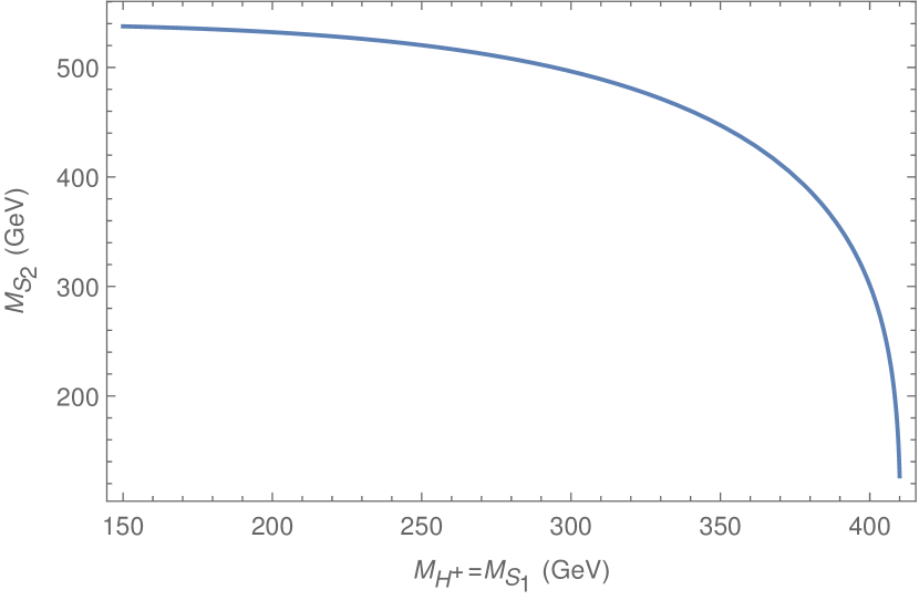
Figure 1: The mass of the neutral Higgs $S_{2}=H^{\prime}/A$ as a function of the common mass of $H^{\pm}$ and the other neutral Higgs, $S_{1}=A/H^{\prime}$, from the sum rule in Eq.(61) with $M_{H}=125\,{\rm GeV}$. Note the considerable sensitivity of $M_{S_{2}}$ to $M_{H^{+}}=M_{S_{1}}$ when the latter is large.

The validity of first-order nondegenerate perturbation theory requires that $\beta^{\prime}\simeq\beta$ so that $|\delta|\ll\beta$. Then $H_{1}\cong H$ and its mass in this model is (from Eq. (9))

$$M_{H_{1}}^{2}\cong M_{H}^{2}=\frac{1}{8\pi^{2}v^{2}}\left(6M_{W}^{4}+3M_{Z}^{4}+M_{H^{\prime}}^{4}+M_{A}^{4}+2M_{H^{\pm}}^{4}-12m_{t}^{4}\right),$$ (61)

where, again, all the masses on the right side of this formula are obtained from zeroth-order perturbation theory, i.e., from $V_{0}$ plus gauge and Yukawa interactions, with $\phi=v$. The way this formula is used to estimate heavy Higgs masses is to fix the left side at $M_{H_{1}}=125\,{\rm GeV}$, thereby determining $(M_{H^{\prime}}^{4}+M_{A}^{4}+2M_{H^{\pm}}^{4})^{1/4}$. Then, as an example, one might fix $M_{H^{\pm}}=M_{A}$ and search for $H_{2}\cong H^{\prime}$ near the mass $M_{H^{\prime}}$ determined by the formula. The sum rule is illustrated in Fig. 1 for $M_{H_{1}}=125\,{\rm GeV}$ and $M_{H^{\pm}}=M_{A}$ or $M_{H^{\prime}}$; the mass of the other neutral scalar is plotted against $M_{H^{\pm}}$. The figure shows that the mass of that scalar is very sensitive to small changes in $M_{H^{\pm}}$ when the latter is large. In the Appendix we compute $M_{H_{1},H_{2}}$ as a function of $\lambda_{3}$, equivalently $M^{2}_{H^{\prime}}$, for $M_{H^{\pm}}=M_{A}=400\,{\rm GeV}$. We shall see then that there can be appreciable differences between $M_{H^{\prime}}$ and the mass eigenvalue $M_{H_{2}}$ even though $M_{H_{1}}\cong M_{H}$ and the angle $\delta\ll\beta$. Thus, the sum rule should be used with some caution in designing searches for large values of $M_{H^{\pm}}=M_{A/H^{\prime}}$. For this case with $M_{H^{\prime}}$ diving to zero for large $M_{H^{\pm}}=M_{A}$, using the eigenvalue $M_{H_{2}}$ of $M_{H_{0^{+}}}$ seems the more reasonable way to estimate its mass; see Fig. 8, e.g.

The diagonalization of ${\cal M}_{H_{0^{+}}}$ and the comparison of our results with those of Ref. [17] are in the Appendix. Here we mention that we find $\delta$ and $\delta/\beta={\cal O}(10^{-2})$ for $\tan\beta\simeq 1/3$–1.0, hence near perfect alignment, as we see next in the Higgs couplings to EW bosons and fermions.

With weak hypercharges of $\textstyle{\frac{1}{2}}$, the EW gauge couplings of the physical Higgs bosons $H_{1}\cong H(125)$, $H_{2}$, $A$ and $H^{\pm}$ are given by:

$${\cal L}_{EW} = ieH^{-}\overleftrightarrow{\partial_{\mu}}H^{+}\left(A^{\mu}+Z^{\mu}\cot 2\theta_{W}\right)$$ (62)

$$+ \frac{e}{\sin 2\theta_{W}}A\overleftrightarrow{\partial_{\mu}}\left(H_{1}\sin\delta-H_{2}\cos\delta\right)Z^{\mu}$$

$$+ \frac{ie}{2\sin\theta_{W}}\left(H^{-}\overleftrightarrow{\partial_{\mu}}(H_{1}\sin\delta-H_{2}\cos\delta+iA)W^{+,\mu}-{\rm h.c.}\right)$$

$$+ (H_{1}\cos\delta+H_{2}\sin\delta)\left(\frac{eM_{W}}{\sin\theta_{W}}W^{+,\mu}W^{-}_{\mu}+\frac{eM_{Z}}{\sin 2\theta_{W}}Z^{\mu}Z_{\mu}\right).$$

The alignment of $H_{1}$ and anti-alignment of $H_{2}$ for small $\delta$ are obvious.

The Yukawa couplings to mass eigenstate quarks and leptons of the physical Higgs bosons dictated by the ${\cal Z}_{2}$ symmetry in Eq. (12) are given by:

$${\cal L}_{Y} = \frac{\sqrt{2}\tan\beta}{v}\sum_{k,l=1}^{3}\left[H^{+}\left(\bar{u}_{kL}V_{kl}\,m_{d_{l}}d_{lR}-\bar{u}_{kR}\,m_{u_{k}}V_{kl}\,d_{lL}+m_{\ell_{k}}\bar{\nu}_{kL}\ell_{kR}\,\delta_{kl}\right)+{\rm h.c.}\right]$$ (63)

$$- \left(\frac{v\cos\beta+H_{1}\cos\beta^{\prime}-H_{2}\sin\beta^{\prime}}{v\cos\beta}\right)\sum_{k=1}^{3}\left(m_{u_{k}}\bar{u}_{k}u_{k}+m_{d_{k}}\bar{d}_{k}d_{k}+m_{\ell_{k}}\bar{\ell}_{k}\ell_{k}\right)$$

$$- \frac{iA\tan\beta}{v}\sum_{k=1}^{3}\left(m_{u_{k}}\bar{u}_{k}\gamma_{5}u_{k}-m_{d_{k}}\bar{d}_{k}\gamma_{5}d_{k}-m_{\ell_{k}}\bar{\ell}_{k}\gamma_{5}\ell_{k}\right).$$

Here, $V$ is the Cabibbo-Kobayashi-Maskawa matrix and fermion masses are to be evaluated at ${\cal O}(300\,{\rm GeV})$. Again the alignment of $H_{1}$ is obvious for small $\delta$.

The charged Higgs couplings in Eq. (63) contribute to $b\to s\gamma$ decays. Ref. [34] studied this transition and bounded $M_{H^{\pm}}>295\,{\rm GeV}$ at the 95% CL in 2HDM with type-II couplings, i.e., in which up-quarks get their mass from $\Phi_{2}$ and down-quarks from $\Phi_{1}$ [35]. Their bound is for $\tan\beta\geq 2$ in such a model. The Yukawa couplings of our model are the variant of type-I with $\Phi_{1}$ and $\Phi_{2}$ interchanged. The bound then corresponds to $\tan\beta\leq\textstyle{\frac{1}{2}}$. In Sec. 3.2 we find a similar bound on $\tan\beta$ from a search for $H^{\pm}$.

We briefly mention two theoretical constraints on this model considered in Ref. [17]. The first is perturbative unitarity. One of its most stringent conditions comes from requiring that the eigenvalue $a_{+}$ of the scattering amplitudes in Ref. [36] obeys the bound

$$a_{+}=\frac{1}{16\pi}\left[3(\lambda_{1}+\lambda_{2})+\sqrt{9(\lambda_{1}-\lambda_{2})^{2}+(2\lambda_{3}+\lambda_{4})^{2}}\right]\leq\textstyle{\frac{1}{2}}.$$ (64)

Note that this is symmetric under $c_{\beta}\leftrightarrow s_{\beta}$. Assuming, e.g, that $M_{H^{\pm}}=M_{A}=400\,{\rm GeV}$, we have

$$a_{+}=\left\{\begin{array}[]{l}0.38\,\,{\rm for}\,\,\tan\beta=\textstyle{\frac{1}{2}}\\ 0.82\,\,{\rm for}\,\,\tan\beta=\textstyle{\frac{1}{3}}\end{array}\right.$$ (65)

The second constraint comes from the oblique parameters $S,T$ [37, 38, 39, 40, 41, 42]. We note here that the contribution to $T$ from the Higgs scalars in this model vanishes identically when $\lambda_{4}=\lambda_{5}$ [43, 44]. For this reason, we often assume $M_{H^{\pm}}=M_{A}$ in the phenomenological considerations of Sec. 3. The constraints following from the $S$-parameter will be discussed there as well.

3. Experimental constraints and opportunities

In this section, we discuss constraints from precision EW measurements at LEP and searches for new charged and neutral Higgs bosons at the LHC and, finally, we summarize targets of opportunity at the LHC.

3.1 Precision Electroweak Constraints

The constraints from $Z$ and $W$ boson properties [45], parameterized by $S$ and $T$ are independent of the choice of Yukawa couplings for the 2HDM. We follow Ref. [17] to evaluate the contributions of the new Higgses to these parameters which included the (formally) two-loop effect of vertex corrections which arise due to the potentially large quartic couplings. The general form of these corrections is [46]

$$S_{\Phi}\! = \!-\frac{1}{4\pi}\left[\left(1+\delta_{\gamma Z}^{H^{\pm}}\right)^{2}F^{\prime}_{\Delta}(M_{H^{\pm}},M_{H^{\pm}})-\sum_{i=1,2}\left(g_{H_{i}AZ}+\delta_{Z}^{H_{i}}\right)^{2}F^{\prime}_{\Delta}(M_{H_{i}},M_{A})\right]\,,$$

$$T_{\Phi}\! = \!-\frac{\sqrt{2}G_{F}}{16\pi^{2}\alpha_{\rm EM}}\ \Bigg{\{}-\left(1+\delta_{W}^{A}\right)^{2}F_{\Delta}(M_{A},M_{H^{\pm}})$$

$$+\sum_{i=1,2}\left[\left(g_{H_{i}AZ}+\delta_{Z}^{H_{i}}\right)^{2}F_{\Delta}(M_{H_{i}},M_{A})-\left(g_{H_{i}H^{-}W^{+}}+\delta_{W}^{H_{i}}\right)^{2}F_{\Delta}(M_{H_{i}},M_{H^{\pm}})\right]\Bigg{\}}\;,\quad$$

where $\delta_{V}^{H}$ is the vertex correction to the coupling of the vector boson $V$ to Higgs boson $H$ (see Ref. [17]) and $F^{\left(\prime\right)}_{\Delta}\left(M_{1},M_{2}\right)$ are the bubble-graph integrals given in Ref. [47]. As noted, the Higgs contribution to $T$ vanishes in this model when $M_{H^{\pm}}=M_{A}$.

The regions of $\tan\beta$–$M_{H^{\pm}}$ parameter space allowed by precision EW data for the cases $M_{H^{+}}=M_{A}$ and $M_{H^{+}}=M_{H^{\prime}}$ are shown in Fig. 2. The mass of the lone neutral scalar in either of these scenarios is taken from the sum rule (61); see Fig. 1. The axes in Fig. 2 are chosen to span the parameter space technically available to the model after direct LEP searches. The lower bound of $70\,{\rm GeV}$ corresponds to the LEP search for charged Higgses [48]. The upper limit of $410\,{\rm GeV}$ is chosen to avoid the region of low $M_{H^{\prime}}$ or $M_{A}$ in Fig. 1. For $M_{H^{\pm}}=M_{H^{\prime}}$, the shared mass must be greater than about $315\,{\rm GeV}$ to satisfy EW precision data constraints at the $1\sigma$ level, and the higher masses allow for smaller values of $\tan\beta$. In the $M_{H^{+}}=M_{A}$ case, a similar region in shared mass and $\tan\beta$ is allowed, but there is a second region within 1$\sigma$ at low common mass and $\tan\beta$. In fact, nearly the entire possible mass range is allowed at the $2\sigma$ level for $\tan\beta>0.2$. We shall see below in Fig. 6 that a CMS search at $8\,{\rm TeV}$ for a charged Higgs boson decaying to $t\bar{b}$ requires $\tan\beta\mathrel{\hbox to0.0pt{\raise 2.20013pt\hbox{$<$}\hss}{\lower 2.20013pt\hbox{$\sim$}}}0.5$ for $180<M_{H^{\pm}}<500\,{\rm GeV}$ [49].

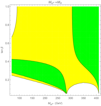
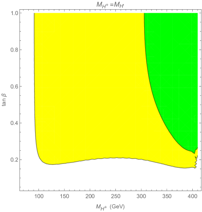
Figure 2: The constraints on the type-I scale-invariant 2HDM arising from precision electroweak measurements. The green (yellow) regions indicate $1\sigma$ ($2\sigma$) agreement with precision data. In the left panel $M_{H^{+}}=M_{A}$, which also enforces that the scalars’ contribution $T_{\Phi}$ to the $T$-parameter vanishes. In the right panel $M_{H^{+}}=M_{H^{\prime}}$ for which $T_{\Phi}\neq 0$. The remaining neutral scalar’s mass is set by Eq. (61).

3.2 Direct Searches at the LHC

In the alignment limit (small $\delta/\beta$), the Yukawa couplings of the new charged and neutral Higgs bosons are proportional to $\tan\beta$. The strong alignment renders ineffective existing searches for such Higgses in weak boson final states, specifically $H_{2}\simeq H^{\prime}$ and $A\to W^{+}W^{-}$, $ZZ$. At the same time, it may strengthen searches in fermionic final states. Reference production cross sections for the new Higgses for several potentially important processes are shown in Figs. 3,4. Note that all the single-Higgs production cross sections which may be efficient in the alignment limit are proportional to $\tan^{2}\beta$.

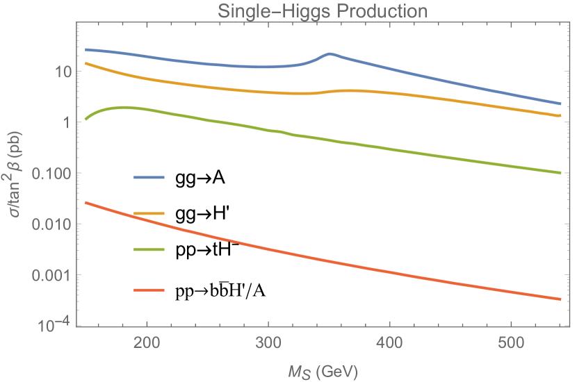
Figure 3: The cross sections for single Higgs production processes in the alignment limit ($\delta\to 0$) with the dependence on $\tan\beta$ scaled out. Both charged Higgs states are included in $pp\to tH^{-}$.

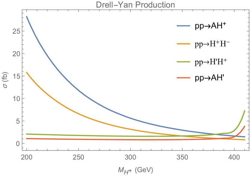
Figure 4: The cross sections for Drell-Yan production of Higgs pairs in the alignment limit ($\delta\to 0$). They are independent of $\tan\beta$. $M_{H^{\pm}}=M_{A}$ is assumed, with $M_{H^{\prime}}$ taken from Eq.(61). The sharp increase at large $M_{H^{\pm}}$ is due to the rapid decrease of $M_{H^{\prime}}$ there; see Fig. 1. For the case $M_{H^{\pm}}=M_{H^{\prime}}$, simply interchange the labels $A$ and $H^{\prime}$ in the figure.

Among heavy scalars, the most promising search is for $tH^{\pm}$-associated production, with $H^{+}\to t\bar{b}$. The subprocess for this is $gb(\bar{b})\to tH^{-}\,(\bar{t}H^{+})$. The most stringent constraint so far on this channel is from the CMS search at $8\,{\rm TeV}$ [49]. In the aligned limit, the other potentially important decay mode is $H^{\pm}\to W^{\pm}H^{\prime}$ or $W^{\pm}A$, whichever neutral Higgs is lighter. That neutral Higgs decays mainly to $\bar{b}b$. Fig. 5 shows the dependence of the branching ratio $B(H^{+}\to t\bar{b})$ as a function of $M_{H^{+}}$ and $\tan\beta$. In this figure, $M_{H^{+}}=M_{A}$ or $M_{H^{\prime}}$ and the other neutral scalar’s mass is given by the sum rule (61). There has been no dedicated search yet for $H^{\pm}\to W^{\pm}H^{\prime}/A$. However, the final state for this decay mode, $tH^{\pm}\to tW^{\pm}H^{\prime}/A\to tW^{\pm}\bar{b}b$, is similar to that of $tH^{\pm}\to tt\bar{b}\to tW^{\pm}\bar{b}b$. Therefore, we conservatively assume that it contributes with equal acceptance to the search at CMS so that the branching ratio of $B(tH^{\pm}\to tW^{\pm}\bar{b}b)=1$. The signal rate then scales as for the single Higgs production, $\sigma\cdot B\propto\tan^{2}\beta$.

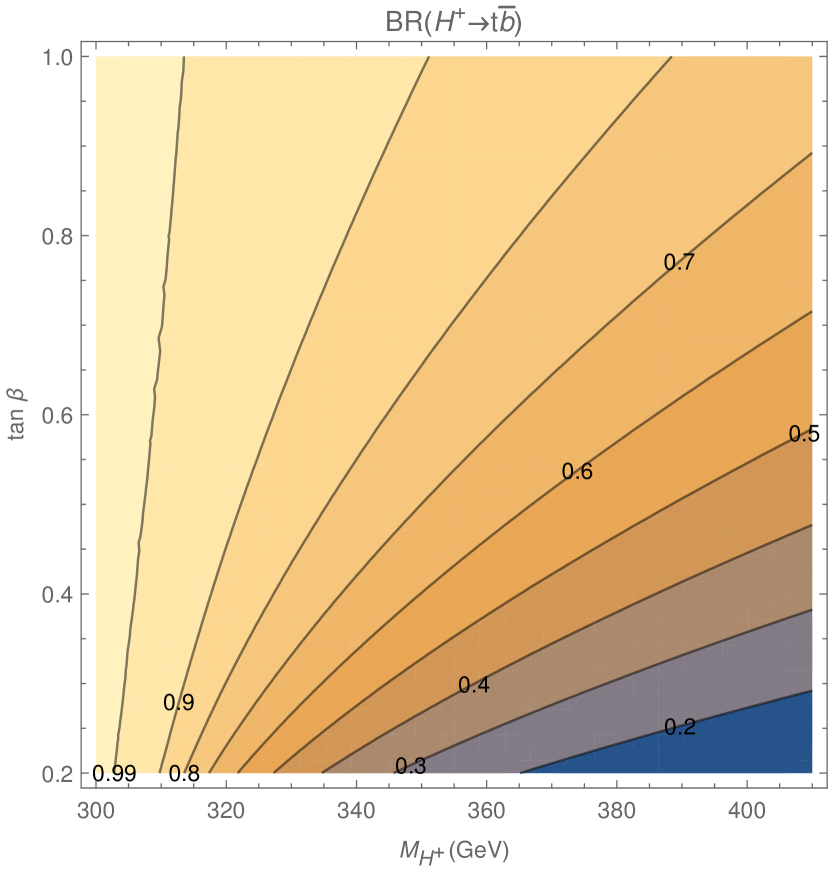
Figure 5: The branching ratio $B(H^{+}\to t\bar{b})$ as a function of $M_{H^{+}}$ and $\tan\beta$. The only other significant decay mode is $H^{+}\to W^{+}H^{\prime}/A$. It is assumed that $M_{H^{+}}=M_{A}$ or $M_{H^{\prime}}$; the other neutral scalar’s mass is then given by Eq. (61).

Because CMS has reported unfolded bounds on $\sigma\cdot B$ for this final state, we are able to recast the search from its type-II 2HDM form into bounds on our type-I model. We show the constraints on $\tan\beta$ as a function of $M_{H^{+}}$ in Fig. 6. As did CMS, we extrapolated linearly between points at which cross section limits were reported.

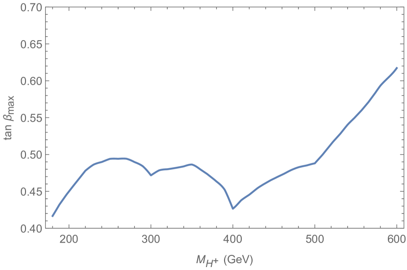
Figure 6: Constraints on $\tan\beta$ in any type-I 2HDM à la the model of Sec. 2 from a CMS search at $8\,{\rm TeV}$ for charged Higgs production in association with another top quark and decaying to $t\bar{b}$ [49]. The kinks in this plot occur at the data points provided by CMS, and arise due to linear interpolation of the excluded cross section for intermediate values of charged Higgs mass.

Further constraints can come from searches for neutral Higgs bosons produced in gluon fusion and decaying to top, bottom or tau pairs. From the sum rule in Eq. (61), the heaviest $H^{\prime}$ or $A$ can be is almost $540\,{\rm GeV}$ when all other masses are $\sim 100\,{\rm GeV}$. An ATLAS search at $8\,{\rm TeV}$ [50] for resonant production of $\bar{t}t$ has been performed only for scalars heavier than $500\,{\rm GeV}$ because of the complexity of interference effects in regions near threshold where off-shell tops become important in heavy Higgs decays. A neutral scalar mass of $M_{H^{\prime}}=500\,{\rm GeV}$ corresponds to $M_{H^{\pm}}=M_{A}=295\,{\rm GeV}$. In principle, such searches are sensitive to the full mass range within $1\sigma$ at lower mass and $\tan\beta$ in the left panel of Fig. 2. The case $M_{H^{\pm}}=M_{H}=295\,{\rm GeV}$ is within $2\sigma$ of Fig,2 and should not be ignored out of hand. This particular search is fairly difficult to recast because the analysis was performed primarily in terms of signal strength in a 2HDM. Using the “signal” rate quoted in auxiliary material together with the constrained signal strength leads to constraints at fixed $M_{A}=500\,{\rm GeV}$ of $\sigma\cdot B<0.32$–$1.69\,{\rm pb}$, corresponding to $\tan\beta<0.62$–$1.02$ in our model. For $M_{H^{\prime}}=500\,{\rm GeV}$, the limits are $\sigma\cdot B<0.085$–$0.40\,{\rm pb}$, corresponding to $\tan\beta<0.59-0.91$. Choosing even the smallest of these bounds on $\tan\beta$, this search does not reach the $1\sigma$ region at low $M_{H^{\pm}}=M_{A}$ in Fig. 2.

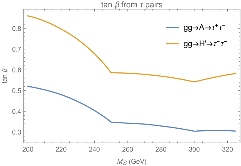
Figure 7: The constraints on $\tan\beta$ in the model of Sec. 2 from the ATLAS search at $13\,{\rm TeV}$ for a neutral Higgs $S=H_{2},A$ decaying to $\tau^{+}\tau^{-}$ [51]. They apply only to the lighter neutral Higgs because decays to light fermions are quickly overwhelmed by, e.g., $A\to H_{2}Z$ or $A\to\bar{t}t$ when the channels open.

A search at $13\,{\rm TeV}$ for production of a neutral scalar in association with a $\bar{b}b$ pair and decaying to another $\bar{b}b$ pair in the mass range $300$–$1300\,{\rm GeV}$ has been carried out by CMS [52]. It is not appreciably sensitive to these models, as the bottom Yukawa coupling is not enhanced as it is in the models targeted by this analysis. The largest $\bar{b}b$-associated new Higgs production cross section in our model, independent of subsequent decay branching ratios, is already sub-femtobarn for $\tan\beta=1$ and, so, is unconstrained by this analysis.

A search for neutral Higgs production — from either gluon fusion or $\bar{b}b$-associated production — with subsequent decays to $\tau^{+}\tau^{-}$ has been performed at $13\,{\rm TeV}$ by ATLAS in the mass range 200–$2250\,{\rm GeV}$ [51]. Gluon fusion production is more promising for our model, with cross sections as large as $20\,{\rm pb}$ for pseudoscalar production at $\tan\beta=1$. Decays to light fermions in this model are quickly overwhelmed by bosonic decays, such as $A\to H_{2}Z$, when accessible. Thus, these searches are capable of constraining only the lighter new neutral scalar in the model. In this limit, the competing decays are to third-generation quarks. The bounds on $tan\beta$ arising from these searches are shown in Fig. 7. Due to the opening of the top quark decay channel, these searches also become ineffective for $M_{H_{2},A}\mathrel{\hbox to0.0pt{\raise 2.20013pt\hbox{$>$}\hss}{\lower 2.20013pt\hbox{$\sim$}}}350\,{\rm GeV}$.

Finally, two searches for a neutral scalar produced in association with $\bar{b}b$ and decaying to $Z$ plus another scalar which itself decays to $\bar{b}b$ or $\tau^{+}\tau^{-}$ has been performed at $13\,{\rm TeV}$ by CMS and ATLAS [53, 54] for models with both scalars’ masses below $1\,{\rm TeV}$. In order that there is adequate splitting between the scalars in our model, either the common scalar mass of the charged and selected neutral scalar must be greater than $\sim 400\,{\rm GeV}$ or less than $\sim 350\,{\rm GeV}$, implying that the heavier scalar’s mass is at least $400\,{\rm GeV}$. From Fig. 3, the greatest production cross section for $pp\to b\bar{b}H^{\prime}/A$ for $\tan\beta=1$ is $\sim 10\,{\rm fb}$. The CMS cross section limits (and comparable ones from ATLAS) for the lighter scalar decaying into $\bar{b}b$ are greater than this largest possible cross section. Limits for decays to $\tau^{+}\tau^{-}$ are a few fb. Including the tau branching ratio of the $H^{\prime}/A$, this limit is also well above the cross section predicted in our model.

A search of interest to ATLAS and CMS is for resonant pair-production of $H(125)$. Unfortunately, the amplitude for $H_{2}\to H_{1}H_{1}$ vanishes in the alignment limit of 2HDM models of type considered here and, so, we expect that it will be a very weak signal. This is related to the vanishing of $H_{2}\to WW$ and $ZZ$ in this limit. As noted in Sec. 2, before the explicit scale-breaking potential $V_{1}$ is turned on, $(H,w^{+},w^{-},z)$ are a degenerate quartet at the critical zero-mass point for electroweak symmetry breaking. Therefore, the three-point amplitude coupling of $H^{\prime}=\lim_{\delta\to 0}H_{2}$ to any pair of these Goldstone bosons vanishes.

3.3 Targets of opportunity at the LHC

We summarize here the likely targets of opportunity at the LHC that we discussed above and remind the reader of some unlikely ones which serve as negative tests of the model we considered. We preface this by recalling that we found that $\tan\beta\mathrel{\hbox to0.0pt{\raise 2.20013pt\hbox{$<$}\hss}{\lower 2.20013pt\hbox{$\sim$}}}\textstyle{\frac{1}{2}}$ and this suppresses certain production rates and decay branching ratios relative to those for the value $\tan\beta=1$ assumed in many 2HDM searches at the LHC.

• Update the search carried out in Ref. [49] for $H^{+}\to t\bar{b}\to W^{+}\bar{b}b$ via the process $g\bar{b}\to\bar{t}H^{+}$ and charge conjugate modes.

• Perform a dedicated search for $g\bar{b}\to\bar{t}H^{+}$ followed by $H^{+}\to W^{+}H_{2}/A\to W^{+}b\bar{b}$. Recall that this has a similar final state as the search above, but includes a resonant $\bar{b}b$ signal.

• Search for single production of $H_{2}/A\to b\bar{b}$ in gluon fusion and possibly in association with $b\bar{b}$. If $H_{2}$ or $A$ are light, in the neighborhood of $200$–$250\,{\rm GeV}$, the decay to $\tau^{+}\tau^{-}$ can be important. It is then also possible that the heavier of the two neutral scalars decays to the lighter one plus a $Z$-boson.

• If possible, search for gluon fusion of $H_{2}/A\to t\bar{t}$ nearer to the $\bar{t}t$ threshold than was done in Ref. [50].

• Search for diboson resonances decaying to $V_{L}V_{L}$ and $V_{L}H$, as discussed in Sec. 2. The mass of such resonances is dictated by the underlying dynamics that produce the scale-invariant potential $V_{0}$ in Eq. (13), dynamics whose energy scale is not specified in the model.

• Drell-Yan production of $H^{\pm}A$, $H^{\pm}H_{2}$, $H_{2}A$ and $H^{+}H^{-}$ are at most a few femtobarns and may, therefore, be more difficult targets than $gg\to H_{2},A$. On the other hand, these cross sections have no $\tan^{2}\beta$ suppression.

• Gluon fusion of $H_{2}/A\to\gamma\gamma$ may be too small to be detected because of the $\tan^{2}\beta$ suppression. If $M_{H_{2}/A}<2m_{t}$, the scalar’s dominant mode may be to $\bar{b}b$. Then $\sigma(gg\to H_{2}/A)B(H_{2}/A\to\gamma\gamma)\propto\tan^{2}\beta$, not $\tan^{4}\beta$, so there is some hope.

• The alignment of the 125 GeV Higgs strongly suppresses the decays of $H_{2}$ and $A$ to $W^{+}W^{-}$ and $ZZ$, as well as $WW$ and $ZZ$ fusion of $H_{2}$ and $A$, providing a negative test of the model.

• The decay rate for $H_{2}=\lim_{\delta\to 0}H_{2}\to HH$ is suppressed by $\delta^{2}$, providing another negative test of the model. If this mode is seen, it is inconsistent with the type of model considered here.

4. Conclusion

In conclusion, we have emphasized here that the low mass and apparent Standard-Model couplings to gauge bosons and fermions of $H(125)$ can have the same symmetry origin: it is the pseudo-Goldstone boson of broken scale symmetry, the scalon of Gildener and Weinberg [14], and this stabilizes its mass and its alignment. In the absence of any other example, we conjectured that the GW mechanism is the only way to achieve a truly Higgslike dilaton. We believe this is an important theoretical point. But there is also an important experimental one to make here. The Gildener-Weinberg scalon picture identifies a specific mass range for new, non-SM Higgs bosons, and that mass range is not far above $H(125)$. Therefore, at the LHC, the relatively low region below about $550\,{\rm GeV}$ currently deserves as much attention as has been given to pushing the machine and the detectors to their limits.

Appendix: CP-even masses and comparison with Lee & Pilaftsis

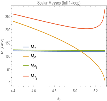
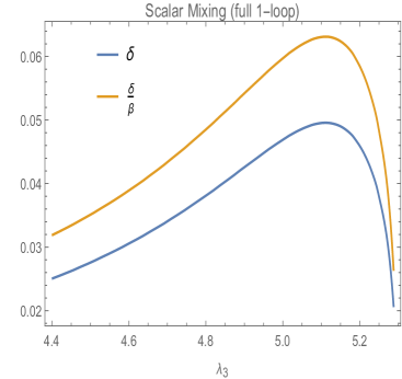
Figure 8: Left: The CP-even Higgs one-loop mass eigenvalues $M_{H_{1}}$ and $M_{H_{2}}$, the tree-level mass $M_{H^{\prime}}=\sqrt{-\lambda_{345}}\,v$ and the one-loop mass $M_{H}$ from Eq. (61) as functions of $\lambda_{3}=(2M_{H^{\pm}}^{2}-M_{H^{\prime}}^{2})/v^{2}$. Here, $\tan\beta=1$ and $M_{H^{\pm}}=M_{A}=400\,{\rm GeV}$ corresponding to $\lambda_{4}=\lambda_{5}=-2.644$. The input $H\cong H_{1}$ mass is $M_{H}=120.5\,{\rm GeV}$, the corresponding initial $M_{H^{\prime}}=231.5\,{\rm GeV}$ and $\lambda_{3}=4.403$. $M_{H^{\prime}}$ vanishes at $\lambda_{3}=2M^{2}_{H^{\pm}}/v^{2}=5.288$. Right: The angle $\delta=\beta-\beta^{\prime}$ and ratio $\delta/\beta$ for $\beta=\pi/4$.

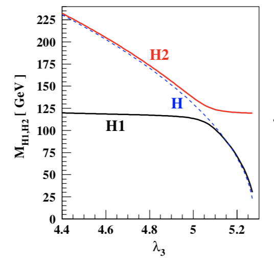
Figure 9: The CP-even Higgs masses $M_{H_{1}},\,M_{H_{2}}$ as functions of $\lambda_{3}=(2M_{H^{\pm}}^{2}-M_{H^{\prime}}^{2})/v^{2}$ for $M_{H^{\pm}}=M_{A}=400\,{\rm GeV}$ and $\tan=1$. The input $H\cong H_{1}$ mass at $\lambda_{3}=4.40$ is $M_{H}=120.5\,{\rm GeV}$. The dashed blue line is the tree-level $M_{H^{\prime}}=\sqrt{-\lambda_{345}}\,v$ with $\lambda_{4}=\lambda_{5}=-M^{2}_{A}/v^{2}=-2.644$. From Ref. [17].

We diagonalized ${\cal M}^{2}_{H_{0^{+}}}$ with elements in Eqs. (2. The Lee-Pilaftsis model) for a range of $\tan\beta\leq 1$ and $M_{H^{\pm}}=M_{A}\simeq 400\,{\rm GeV}$. The general features of our results are fairly insensitive to these choices. The input parameters for the calculation reported here were chosen to be the same as those in Ref. [17], namely, $\tan\beta=1.0$ and $M_{H^{\pm}}=M_{A}=400\,{\rm GeV}$. These masses determine $\lambda_{4}=\lambda_{5}=-M_{A}^{2}/v^{2}=-2.644$. To initiate the calculation, the value $(M_{H})_{i}=120.5\,{\rm GeV}$ was chosen from which, using Eq. (61), $(M_{H^{\prime}})_{i}=231.5\,{\rm GeV}$ and $(\lambda_{3})_{i}=4.403$ were determined; $\lambda_{3}$ was then incremented to the maximum value $(\lambda_{3})_{f}=2M^{2}_{H^{\pm}}/v^{2}=5.288$ at which $M^{2}_{H^{\prime}}=-\lambda_{345}v^{2}$ vanishes. For each value of $\lambda_{3}$, a new value of $M_{H^{\prime}}=\sqrt{-\lambda_{345}}\,v$ is determined and used in the sum rule to update $M_{H}$ in the matrix elements of Eqs. (2. The Lee-Pilaftsis model). Note that it is consistent loop-perturbation theory to use tree-level expressions to compute the nonzero, one-loop value of $M_{H}$.

Fig. 8 shows $M_{H}$ from Eq. (61), the zeroth-order mass $M_{H^{\prime}}$, and the eigenvalues $M_{H_{1},H_{2}}$ (left) and the angle $\delta=\beta-\beta^{\prime}$ and ratio $\delta/\beta$ (right). In the masses plot, $M_{H_{1}}/M_{H}\cong 1.03$ for all $\lambda_{3}$; $M_{H_{2}}$ starts off about 10% greater than $M_{H^{\prime}}$ and increases to 70% greater when $M_{H^{\prime}}=M_{H}$ at $\lambda_{3}\cong 5.04$. Then $M_{H_{2}}$ diverges upward while $M_{H^{\prime}}$ plunges to zero. The mixing angle $\delta$ (right), which measures the deviation from perfect alignment of $H_{1}$, is just several percent and a small fraction of $\beta$; $\delta/\beta$ has a broad maximum of about 6% near $\lambda_{3}=5.11$. For this choice of input parameters, then, the alignment of the $125\,{\rm GeV}$ Higgs boson $H$ is nearly perfect.

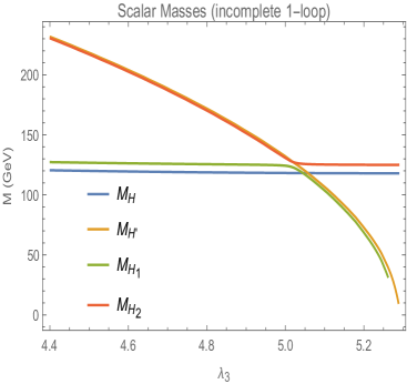
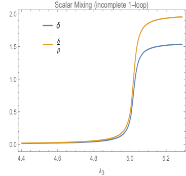
Figure 10: Left: The CP-even Higgs masses, with input parameters of Fig 8, except that the eigenvalues $M^{2}_{H_{1},\,H_{2}}$ of $M^{2}_{H^{0^{+}}}$ were calculated using the tree-level extremal conditions $2\lambda_{1}+\lambda_{345}\tan^{2}\beta=2\lambda_{2}+\lambda_{345}\cot^{2}\beta=0$. Right: The angle $\delta=\beta-\beta^{\prime}$ (solid) and ratio $\delta/\beta$ (dashed) for $\beta=\pi/4$.

These results are qualitatively similar to those obtained by LP in Ref. [17], but only up to $\lambda_{3}\simeq 4.8$; see Fig. 9. The LP paper was submitted in April 2012, before the announcement of the discovery of $H(125)$ and before a more precise value of its mass had been announced. Hence, it appears, their chosen input value of $M_{H}=120.5\,{\rm GeV}$. Up to $\lambda_{3}\simeq 4.9$, $H_{2}\cong H^{\prime}$ with the tree-level mass $M_{H_{2}}\cong M_{H^{\prime}}=\sqrt{-\lambda_{345}}\,v=\sqrt{2M^{2}_{H^{\pm}}-\lambda_{3}}\,v$. Meanwhile, $H_{1}\cong H$ with $M_{H_{1}}$ given by Eq. (61) is almost constant at $120\,{\rm GeV}$. In this region, $\delta$ is small and $\beta^{\prime}\cong\beta=\pi/4$. Beyond $\lambda_{3}\simeq~{}4.9$, there is a clear deviation from this behavior and a level crossing which LP identify as occurring at $\lambda_{3}^{c}\cong 5.06$. Above $\lambda_{3}^{c}$, $M_{H_{2}}\cong 120\,{\rm GeV}$ while $M_{H_{1}}$ and $M_{H^{\prime}}$ coalesce and fall to zero at $(\lambda_{3})_{f}=5.288$. Here, $\delta\simeq\pi/2=2\beta$, and the LP calculation is well past the point of reliable first-order perturbation theory.

We cannot reproduce the level crossing seen in Fig. 9 using the ${\cal M}^{2}_{H_{0^{+}}}$ matrix elements in Eq. (2. The Lee-Pilaftsis model). However, we found that we could by using the tree-level extremal conditions, $\lambda_{1}+\textstyle{\frac{1}{2}}\lambda_{345}\tan^{2}\beta=\lambda_{2}+\textstyle{\frac{1}{2}}\lambda_{345}\cot^{2}\beta=0$. The result is illustrated in Fig. 10. The level crossing in the ${\cal M}_{H_{0^{+}}}$ eigenvalues occurs at the same place as in LP’s calculation. Because it is much more rapid in our calculation than in LP’s, we can pinpoint it at $\lambda_{3}=5.04$. We do not know if this is why LP obtained their level crossing. But there is no doubt that using the tree-level extremal conditions in ${\cal M}^{2}_{H_{0^{+}}}$ is not consistent loop-perturbation theory and, in fact, the results are renormalization-scale dependent.

References

- [1] ATLAS Collaboration, G. Aad et. al., “Observation of a new particle in the search for the Standard Model Higgs boson with the ATLAS detector at the LHC,” Phys.Lett. B716 (2012) 1–29, 1207.7214.
- [2] CMS Collaboration, S. Chatrchyan et. al., “Observation of a new boson at a mass of 125 GeV with the CMS experiment at the LHC,” Phys.Lett. B716 (2012) 30–61, 1207.7235.
- [3] Particle Data Group Collaboration, M. Tanabashi et. al., “Review of Particle Physics,” Phys. Rev. D98 (2018), no. 3, 030001.
- [4] ATLAS Collaboration, T. A. collaboration, “Combined measurements of Higgs boson production and decay using up to 80 fb-1 of proton–proton collision data at 13 TeV collected with the ATLAS experiment,”.
- [5] CMS Collaboration, A. M. Sirunyan et. al., “Observation of H production,” Phys. Rev. Lett. 120 (2018), no. 23, 231801, 1804.02610.
- [6] ATLAS Collaboration, M. Aaboud et. al., “Observation of Higgs boson production in association with a top quark pair at the LHC with the ATLAS detector,” 1806.00425.
- [7] J. F. Gunion and H. E. Haber, “The CP conserving two Higgs doublet model: The Approach to the decoupling limit,” Phys. Rev. D67 (2003) 075019, hep-ph/0207010.
- [8] M. Carena, I. Low, N. R. Shah, and C. E. M. Wagner, “Impersonating the Standard Model Higgs Boson: Alignment without Decoupling,” JHEP 04 (2014) 015, 1310.2248.
- [9] P. S. Bhupal Dev and A. Pilaftsis, “Maximally Symmetric Two Higgs Doublet Model with Natural Standard Model Alignment,” JHEP 12 (2014) 024, 1408.3405. [Erratum: JHEP11,147(2015)].
- [10] P. S. B. Dev and A. Pilaftsis, “Natural Standard Model Alignment in the Two Higgs Doublet Model,” J. Phys. Conf. Ser. 631 (2015), no. 1, 012030, 1503.09140.
- [11] K. Benakli, M. D. Goodsell, and S. L. Williamson, “Higgs alignment from extended supersymmetry,” Eur. Phys. J. C78 (2018), no. 8, 658, 1801.08849.
- [12] K. Benakli, Y. Chen, and G. Lafforgue-Marmet, “Predicting Alignment in a Two Higgs Doublet Model,” 2018. 1812.02208.
- [13] S. R. Coleman and E. J. Weinberg, “Radiative Corrections as the Origin of Spontaneous Symmetry Breaking,” Phys. Rev. D7 (1973) 1888–1910.
- [14] E. Gildener and S. Weinberg, “Symmetry Breaking and Scalar Bosons,” Phys. Rev. D13 (1976) 3333.
- [15] S. Weinberg, “Perturbative Calculations of Symmetry Breaking,” Phys. Rev. D7 (1973) 2887–2910.
- [16] W. A. Bardeen, “On naturalness in the standard model,” in Ontake Summer Institute on Particle Physics Ontake Mountain, Japan, August 27-September 2, 1995. 1995.
- [17] J. S. Lee and A. Pilaftsis, “Radiative Corrections to Scalar Masses and Mixing in a Scale Invariant Two Higgs Doublet Model,” Phys. Rev. D86 (2012) 035004, 1201.4891.
- [18] K. Hashino, S. Kanemura, and Y. Orikasa, “Discriminative phenomenological features of scale invariant models for electroweak symmetry breaking,” Phys. Lett. B752 (2016) 217–220, 1508.03245.
- [19] W. D. Goldberger, B. Grinstein, and W. Skiba, “Distinguishing the Higgs boson from the dilaton at the Large Hadron Collider,” Phys.Rev.Lett. 100 (2008) 111802, 0708.1463.
- [20] B. Bellazzini, C. Csaki, J. Hubisz, J. Serra, and J. Terning, “A Higgslike Dilaton,” Eur. Phys. J. C73 (2013), no. 2, 2333, 1209.3299.
- [21] J. Serra, “A higgs-like dilaton: viability and implications,” EPJ Web Conf. 60 (2013) 17005, 1312.0259.
- [22] B. Bellazzini, C. Csáki, and J. Serra, “Composite Higgses,” Eur.Phys.J. C74 (2014), no. 5, 2766, 1401.2457.
- [23] D. M. Ghilencea, Z. Lalak, and P. Olszewski, “Standard Model with spontaneously broken quantum scale invariance,” Phys. Rev. D96 (2017), no. 5, 055034, 1612.09120.
- [24] P. Hernandez-Leon and L. Merlo, “Distinguishing A Higgs-Like Dilaton Scenario With A Complete Bosonic Effective Field Theory Basis,” Phys. Rev. D96 (2017), no. 7, 075008, 1703.02064.
- [25] B. Bellazzini, C. Csaki, J. Hubisz, J. Serra, and J. Terning, “A Naturally Light Dilaton and a Small Cosmological Constant,” Eur. Phys. J. C74 (2014) 2790, 1305.3919.
- [26] F. Coradeschi, P. Lodone, D. Pappadopulo, R. Rattazzi, and L. Vitale, “A naturally light dilaton,” JHEP 11 (2013) 057, 1306.4601.
- [27] S. L. Glashow and S. Weinberg, “Natural Conservation Laws for Neutral Currents,” Phys. Rev. D15 (1977) 1958.
- [28] K. Lane and L. Pritchett, “Heavy Vector Partners of the Light Composite Higgs,” Phys. Lett. B753 (2016) 211–214, 1507.07102.
- [29] T. Appelquist, Y. Bai, J. Ingoldby, and M. Piai, “Spectrum-doubled Heavy Vector Bosons at the LHC,” JHEP 01 (2016) 109, 1511.05473.
- [30] G. Brooijmans et. al., “Les Houches 2015: Physics at TeV colliders - new physics working group report,” in 9th Les Houches Workshop on Physics at TeV Colliders (PhysTeV 2015) Les Houches, France, June 1-19, 2015. 2016. 1605.02684.
- [31] V. Cavaliere, R. Les, T. Nitta, and K. Terashi, “HE-LHC prospects for diboson resonance searches and electroweak WW/WZ production via vector boson scattering in the semi-leptonic final states,” 1812.00841.
- [32] M. Carena and H. E. Haber, “Higgs boson theory and phenomenology,” Prog. Part. Nucl. Phys. 50 (2003) 63–152, hep-ph/0208209.
- [33] C. T. Hill, “Is the Higgs Boson Associated with Coleman-Weinberg Dynamical Symmetry Breaking?,” Phys. Rev. D89 (2014), no. 7, 073003, 1401.4185.
- [34] M. Misiak et. al., “Estimate of at ,” Phys. Rev. Lett. 98 (2007) 022002, hep-ph/0609232.
- [35] G. C. Branco, P. M. Ferreira, L. Lavoura, M. N. Rebelo, M. Sher, and J. P. Silva, “Theory and phenomenology of two-Higgs-doublet models,” Phys. Rept. 516 (2012) 1–102, 1106.0034.
- [36] S. Kanemura, T. Kubota, and E. Takasugi, “Lee-Quigg-Thacker bounds for Higgs boson masses in a two doublet model,” Phys. Lett. B313 (1993) 155–160, hep-ph/9303263.
- [37] D. C. Kennedy and B. W. Lynn, “Electroweak Radiative Corrections with an Effective Lagrangian: Four Fermion Processes,” Nucl. Phys. B322 (1989) 1.
- [38] M. E. Peskin and T. Takeuchi, “A new constraint on a strongly interacting Higgs sector,” Phys. Rev. Lett. 65 (1990) 964–967.
- [39] M. E. Peskin and T. Takeuchi, “Estimation of oblique electroweak corrections,” Phys. Rev. D46 (1992) 381–409.
- [40] M. Golden and L. Randall, “Radiative corrections to electroweak parameters in technicolor theories,” Nucl. Phys. B361 (1991) 3–23.
- [41] B. Holdom and J. Terning, “Large corrections to electroweak parameters in technicolor theories,” Phys. Lett. B247 (1990) 88–92.
- [42] G. Altarelli, R. Barbieri, and S. Jadach, “Toward a model independent analysis of electroweak data,” Nucl. Phys. B369 (1992) 3–32.
- [43] R. A. Battye, G. D. Brawn, and A. Pilaftsis, “Vacuum Topology of the Two Higgs Doublet Model,” JHEP 08 (2011) 020, 1106.3482.
- [44] A. Pilaftsis, “On the Classification of Accidental Symmetries of the Two Higgs Doublet Model Potential,” Phys. Lett. B706 (2012) 465–469, 1109.3787.
- [45] Particle Data Group Collaboration, C. Patrignani et. al., “Review of Particle Physics,” Chin. Phys. C40 (2016), no. 10, 100001.
- [46] D. Toussaint, “Renormalization Effects From Superheavy Higgs Particles,” Phys. Rev. D18 (1978) 1626.
- [47] S. Kanemura, Y. Okada, H. Taniguchi, and K. Tsumura, “Indirect bounds on heavy scalar masses of the two-Higgs-doublet model in light of recent Higgs boson searches,” Phys. Lett. B704 (2011) 303–307, 1108.3297.
- [48] LEP, DELPHI, OPAL, ALEPH, L3 Collaboration, G. Abbiendi et. al., “Search for Charged Higgs bosons: Combined Results Using LEP Data,” Eur. Phys. J. C73 (2013) 2463, 1301.6065.
- [49] CMS Collaboration, V. Khachatryan et. al., “Search for a charged Higgs boson in pp collisions at TeV,” JHEP 11 (2015) 018, 1508.07774.
- [50] ATLAS Collaboration, M. Aaboud et. al., “Search for Heavy Higgs Bosons Decaying to a Top Quark Pair in Collisions at with the ATLAS Detector,” Phys. Rev. Lett. 119 (2017), no. 19, 191803, 1707.06025.
- [51] ATLAS Collaboration, M. Aaboud et. al., “Search for additional heavy neutral Higgs and gauge bosons in the ditau final state produced in 36 fb−1 of pp collisions at TeV with the ATLAS detector,” JHEP 01 (2018) 055, 1709.07242.
- [52] CMS Collaboration, A. M. Sirunyan et. al., “Search for beyond the standard model Higgs bosons decaying into a pair in pp collisions at 13 TeV,” 1805.12191.
- [53] CMS Collaboration, V. Khachatryan et. al., “Search for neutral resonances decaying into a Z boson and a pair of b jets or leptons,” Phys. Lett. B759 (2016) 369–394, 1603.02991.
- [54] ATLAS Collaboration, M. Aaboud et. al., “Search for a heavy Higgs boson decaying into a boson and another heavy Higgs boson in the final state in collisions at TeV with the ATLAS detector,” Phys. Lett. B783 (2018) 392–414, 1804.01126.
- [55] ATLAS Collaboration, M. Aaboud et. al., “Search for charged Higgs bosons decaying into top and bottom quarks at = 13 TeV with the ATLAS detector,” 1808.03599.