Boundaries of Baumslag-Solitar Groups

Abstract.

A $\mathcal{Z}$-structure on a group $G$ was introduced by Bestvina in order to extend the notion of a group boundary beyond the realm of CAT(0) and hyperbolic groups. A refinement of this notion, introduced by Farrell and Lafont, includes a $G$-equivariance requirement, and is known as an $\mathcal{EZ}$-structure. The general questions of which groups admit $\mathcal{Z}$- or $\mathcal{EZ}$-structures remain open. In this paper we add to the current knowledge by showing that all Baumslag-Solitar groups admit $\mathcal{EZ}$-structures and all generalized Baumslag-Solitar groups admit $\mathcal{Z}$-structures.

1. Introduction

In [Bes96], Bestvina introduced the concept of a $\mathcal{Z}$-structure on a group $G$ to provide an axiomatic treatment of group boundaries. Roughly speaking, the definition requires $G$ to act geometrically (properly, cocompactly, by isometries) on a “nice” space $X$ and for that space to admit a nice compactification $\overline{X}$ (a $\mathcal{Z}$-compactification). In addition, it is required that translates of compact subsets of $X$ get small in $\overline{X}$ — a property called the nullity condition. Adding visual boundaries to CAT(0) spaces and Gromov boundaries to appropriately chosen Rips complexes provide the model examples. To admit a $\mathcal{Z}$-structure, it is necessary that a group $G$ admits a finite $K(G,1)$ complex (a Type F group). Bestvina posed the still open question as to whether or not every Type F group admits a $\mathcal{Z}$-structure.

In [Bes96], the Baumslag-Solitar group $BS\left(1,2\right)$ was put forward as a non-hyperbolic, non-CAT(0) group that, nevertheless, admits a $\mathcal{Z}$-structure. Baumslag-Solitar groups $BS\left(1,n\right)$ behave similarly, but from the beginning, the status of general Baumslag-Solitar groups $BS\left(m,n\right)$ was unclear. In this paper we resolve that issue in a strong way.

Theorem 1.1.

Every generalized Baumslag-Solitar group admits a $\mathcal{Z}$-structure.

A generalized Baumslag-Solitar group is the fundamental group of a graph of groups with vertex and edge groups $\mathbb{Z}$. By applying work of Whyte [Why01] and a boundary swapping trick (see [Bes96] and [GM18]), it will suffice to show that the actual Baumslag-Solitar groups $BS(m,n)$ admit $\mathcal{Z}$-structures. For those groups, we will prove the following stronger theorem.

Theorem 1.2 ($\mathcal{EZ}$-Structures on Baumslag-Solitar Groups).

All Baumslag-Solitar groups, $BS(m,n)$, admit $\mathcal{EZ}$-structures.

Here $\mathcal{EZ}$ stands for “equivariant $\mathcal{Z}$-structure”, a $\mathcal{Z}$-structure in which the group action extends to the boundary. Torsion-free groups (which includes all groups studied in this paper) that admit $\mathcal{EZ}$-structures are known to satisfy the Novikov conjecture ([FL05]). That is one reason to aim for this stronger condition.

2. Background

2.1. Visual Boundaries of CAT(0) Spaces

In this section, we review the definition of CAT(0) spaces and the visual boundary as we will use these as a starting point for $\mathcal{EZ}$-structures on $BS(m,n)$. For a more thorough treatment of CAT(0) spaces, see [BH99].

Definition 2.1.

A geodesic metric space $(X,d)$ is a CAT(0) space if all of its geodesic triangles are no fatter than their corresponding Euclidean comparison triangles. That is, if $\Delta(p,q,r)$ is any geodesic triangle in $X$ and $\overline{\Delta}(\overline{p},\overline{q},\overline{r})$ is its comparison triangle in $\mathbb{E}^{2}$, then for any $x,y\in\Delta$ and the comparison points $\overline{x},\overline{y}\in\overline{\Delta}$, then $d(x,y)\leq d_{\mathbb{E}}(\overline{x},\overline{y})$.

Example 1.

Basic examples of CAT(0) spaces include:

• $\mathbb{R}^{n}$ equipped with the Euclidean metric is a CAT(0) space as all geodesic triangles are already Euclidean and hence no fatter than their comparison triangles.

• A tree, $T$, is a CAT(0) space since all geodesic triangles are degenerate and thus have no thickness associated to them.

• If $X$ and $Y$ are CAT(0), spaces, then $X\times Y$ with the $\ell^{2}$ metric is CAT(0). So, for example, $\mathbb{R}\mathbb{\times}T$ is a CAT(0) space—a fact that will play a significant role in this paper.

A group $G$ that acts properly, cocompactly, and by isometries (also known as a geometric group action) on a proper CAT(0) space is called a CAT(0) group.

Definition 2.2.

The boundary of a proper CAT(0) space $X$, denoted $\partial X$, is the set of equivalence classes of rays, where two rays are equivalent if and only if they are asymptotic. We say that two geodesic rays $\alpha,\alpha^{\prime}:[0,\infty)\to X$ are asymptotic if there is some constant $k$ such that $d(\alpha(t),\alpha^{\prime}(t))\leq k$ for every $t\geq 0$.

If we fix a base point $x_{0}\in X$, each equivalence class of rays in $X$ contains exactly one representative emanating from $x_{0}$. So when $x_{0}$ is chosen, we can view $\partial X$ as the set of all rays in $X$ based at $x_{0}$. We may endow $\overline{X}=X\cup\partial X$, with the cone topology, described below, under which $\partial X$ is a closed subspace of $\overline{X}$ and $\overline{X}$ compact (provided $X$ is proper). Equipped with the topology induced by the cone topology on $\overline{X}$, the boundary is called the visual boundary of $X$; we will denote it by $\partial_{\infty}X$.

The cone topology on $\overline{X}$, denoted $\mathcal{T}(x_{0})$ for $x_{0}\in X$, is generated by the basis $\mathcal{B}=\mathcal{B}_{0}\cup\mathcal{B}_{\infty}$ where $\mathcal{B}_{0}$ consists of all open balls $B(x,r)\subset X$ and $\mathcal{B}_{\infty}$ is the collection of all sets of the form

$$U(c,r,\epsilon)=\{x\in\overline{X}\mid d(x,c(0))>r\text{ and }d(p_{r}(x),c(r))<\epsilon\}$$

where $c:[0,\infty)\rightarrow X$ is any geodesic ray based at $x_{0}$, $r>0$, $\epsilon>0$, and $p_{r}$ is the natural projection of $\overline{X}$ onto $\overline{B}(c(0),r)$.

Example 2.

Boundaries of the simple examples given above are:

• $\partial_{\infty}\mathbb{R}^{n}\simeq S^{n-1}$

• $\partial_{\infty}T$ is compact and $0$-dimensional. If each vertex has degree $\geq 3$, it is a Cantor set $C$. (In order for $T$ to be proper, assume all vertices have finite degree.)

• If $X$ and $Y$ are CAT(0), spaces and $X\times Y$ is given the $\ell^{2}$ metric, then $\partial_{\infty}(X\times Y)\simeq\partial X\ast\partial Y$, the (spherical) join of the two boundaries. For example, $\partial_{\infty}(\mathbb{R}\mathbb{\times}T)$ is homeomorphic to $S^{0}\ast\partial_{\infty}T$; the suspension of a $0$-dimensional set (usually a Cantor set)..

When $G$ is a CAT(0) group acting geometrically on a proper CAT(0) space $X$, we call $\partial_{\infty}X$ a CAT(0) boundary for $G$. For example, since $\mathbb{Z}^{n}$ acts geometrically on $\mathbb{R}^{n}$, it is a CAT(0) group and $S^{n-1}$ is a CAT(0) boundary . The free group on two generators, $F_{2}$, acts geometrically on a four-valent tree, so a CAT(0) boundary for $F_{2}$ is the Cantor set.

The following lemma, which is reminiscent of the Lebesgue covering lemma, will be useful in proving our main theorem.

Lemma 2.3.

Let $(X,d)$ be a proper CAT(0) space and let $\mathcal{U}$ be an open cover of $\overline{X}$. Then there exists a $\delta>0$ so that for every $z\in\partial X$, $U(z,\frac{1}{\delta},\delta)$ lies in an element of $\mathcal{U}$.

Proof.

Since $\partial X$ is compact, there is a finite subcollection $\{U_{1},U_{2},...,U_{k}\}$ of $\mathcal{U}$ that covers $\partial X$. For each $i\in\{1,2,...,k\}$, define a function $\eta_{i}:\partial X\to[0,\infty)$ by $\eta_{i}(z)=\text{sup}\{\epsilon\,|\,U(z,\frac{1}{\epsilon},\epsilon)\subseteq U_{i}\}$. Note that $\eta_{i}$ is continuous and $\eta_{i}(z)>0$ if and only if $z\in U_{i}$. Thus, $\eta:\partial X\to[0,\infty)$ defined by $\eta(z)=\text{max}\{\eta_{i}(z)\}_{i=1}^{k}$ is continuous and strictly positive. Let $\delta^{\prime}$ be the minimum value of $\eta$ and set $\delta=\frac{\delta^{\prime}}{2}$. ∎

2.2. $\mathcal{Z}$-Structures

Boundaries of CAT(0) groups have proven to be useful objects that can help us gain more information about the groups themselves. This led Bestvina to generalize the notion of group boundaries by defining “$\mathcal{Z}$-boundaries” for groups, a topic that we explore now. For more on $\mathcal{Z}$-structures, see [Bes96] and [GM18].

Definition 2.4.

A closed subset $A$ of a space $X$, is a $\mathcal{Z}$-set if there exists a homotopy $H:X\times[0,1]\rightarrow X$ such that $H_{0}=\operatorname*{id}_{X}$ and $H_{t}(X)\subset X-A$ for every $t>0$.

Example 3.

The prototypical $\mathcal{Z}$-set is the boundary of a manifold, or any closed subset of that boundary.

A $\mathcal{Z}$-compactification of a space $X$ is a compactification $\overline{X}$ such that $\overline{X}-X$ is a $\mathcal{Z}$-set in $\overline{X}$.

Example 4.

The addition of the visual boundary to a proper CAT(0) space $X$ gives a $\mathcal{Z}$-compactification $\overline{X}$ of $X$. A simple way to see the visual boundary as a $\mathcal{Z}$-set in $\overline{X}$ is to imagine the homotopy that “reels” points of the boundary in along the geodesic rays.

Definition 2.5.

A $\mathcal{Z}$-structure on a group $G$ is a pair of spaces $(\overline{X},Z)$ satisfying the following four conditions:

1. $\overline{X}$ is a compact AR,

2. $Z$ is a $\mathcal{Z}$-set in $\overline{X}$,

3. $X=\overline{X}-Z$ is a proper metric space on which $G$ acts geometrically, and

4. $\overline{X}$ satisfies the following nullity condition with respect to the $G$-action on $X$: for every compact $C\subseteq X$ and any open cover $\mathcal{U}$ of $\overline{X}$, all but finitely many $G$-translates of $C$ lie in an element of $\mathcal{U}$.

When this definition is satisfied, $Z$ is called a $\mathcal{Z}$-boundary for $G$. If only conditions (1)-(3) are satisfied, the result is called a weak $\mathcal{Z}$-structure. If, in addition to (1)-(4)above, the $G$-action on $X$ extends to $\overline{X}$, the result is called an $\mathcal{EZ}$-structure (equivariant) $\mathcal{Z}$-structure.

Example 5.

The following are the most common examples of $(\mathcal{E})\mathcal{Z}$-structures:

1. If $G$ acts geometrically on a proper CAT(0) space $X$, then $\overline{X}=X\cup\partial_{\infty}X$, with the cone topology, gives an $\mathcal{EZ}$-structure for $G$.

2. In [BM91] it is shown that if $G$ is a hyperbolic group, $P_{\rho}(G)$ is an appropriately chosen Rips complex, and $\partial G$ is the Gromov boundary, then $\overline{P}_{\rho}(G)=P_{\rho}(G)\cup\partial G$ (appropriately topologized) gives an $\mathcal{EZ}$-structure for $G$.

3. Osajda and Przytycki [OP09] have shown that systolic groups admit $\mathcal{EZ}$-structures.

Other classes of groups that admit $\mathcal{Z}$-structures have been addressed by Dahmani [Dah03] (relatively hyperbolic groups), Martin [Mar14] (complexes of groups), Osajda and Przytycki [OP09] (systolic groups), Tirel [Tir11] (free and direct products), and Pietsch [Pie18] (semidirect products with $\mathbb{Z}$ and 3-manifold groups).

Most of the Baumslag-Solitar groups $BS(m,n)$ and generalized Baumslag-Solitar groups do not belong to any of the categories listed above and thus Theorem 1.2 adds an interesting new set of examples to this list.

A few comments are in order regarding the definition of $\mathcal{Z}$-structure. First, Bestvina’s original definition did not explicitly require actions by isometries, but only by covering transformations. As we point out at the end of Section 3.3, there is no loss of generality in requiring actions by isometries. Bestvina also required $\overline{X}$ to be finite-dimensional and the action to be free. Dranishnikov relaxed both of these conditions in [Dra06], and [GM18] shows that nothing is lost in doing so.

We close this section with a few observations about $\mathcal{Z}$-structures. The first makes the nullity condition more intuitive; the second is useful for verifying the nullity condition; and the third can (and will) be used to obtain $\mathcal{Z}$-structures for a broad class of groups without checking each group individually.

Every $\mathcal{Z}$-compactification $\overline{X}$ of a proper metric space $\left(X,d\right)$ is metrizable (see [GM18]), but in general, there is no canonical choice of metric for $\overline{X}$; moreover whichever metric $\overline{d}$ one chooses will be quite different from $d$. Nevertheless, any such choice can be used to give the following intuitive meaning to the nullity condition. The proof is straight-forward general topology.

Lemma 2.6.

Let $(\overline{X},Z)$ be a weak $\mathcal{Z}$-structure as described in Definition 2.5, and let $\overline{d}$ be a metric for $\overline{X}$. Then $(\overline{X},Z)$ satisfies the nullity condition (and hence is a $\mathcal{Z}$-structure) if and only if

$$\text{(\textdagger) for any compact set }C\subseteq X\text{ and }\epsilon>0\text{,all but finitely many }G\text{-translates}$$

$$\text{ of }C\text{{ have }}\overline{d}\text{-diameter less than }\epsilon\text{.}$$

The next lemma allows us to verify the nullity condition without checking every compact subset $C$ of $X$.

Lemma 2.7.

Let $X$ be a proper metric space admitting a proper cocompact action by $G$ and let $\left(\overline{X},\overline{d}\right)$ be a $\mathcal{Z}$-compactification of $X$ If $C$ is a compact subset of $X$ with the property that $GC=X$ and the nullity condition is satisfied for $C$, then the nullity condition is satisfied for all compact subsets of $X$.

Proof.

Choose $\epsilon>0$ and let $K\subseteq X$ be an arbitrary compact set. By properness and the hypothesis, there are finitely many translates of $C$ that cover $K$, that is $K\subseteq g_{1}C\cup g_{2}C\cup...\cup g_{n}C$ for $g_{i}\in G$. Since $C$ satisfies the nullity condition, all but finitely many $G$ translates of $C$ have $\overline{d}$-diameter less than $\frac{\epsilon}{n}$. If we consider any translate $gK$, then $gK\subseteq gg_{1}C\cup gg_{2}C\cup...\cup gg_{n}C$. Only finitely many $gg_{i}C$ for $g\in G$ have diameter greater than $\frac{\epsilon}{n}$ and thus only finitely many $gK$ have diameter greater than $n\frac{\epsilon}{n}=\epsilon$. ∎

The following useful fact is often referred to as the “boundary swapping trick”.

Proposition 2.8.

[Bes96, GM18] Suppose $G$ and $H$ are quasi-isometric groups that act geometrically on proper metric ARs $X$ and $Y$, respectively, and $Y$ can be compactified to a $\mathcal{Z}$-structure $\left(\overline{Y},Z\right)$ for $H$, then $X$ can be compactified by addition of the same boundary to obtain a $\mathcal{Z}$-structure $\left(\overline{X},Z\right)$ for $G$.

3. $\mathcal{Z}$-structures on generalized Baumslag-Solitar Groups

A Baumslag-Solitar group $BS(m,n)$ is a two generator, one relator group admitting a presentation of the form

$$BS(m,n)=\left\langle s,t\,|\,ts^{m}t^{-1}=s^{n}\right\rangle.$$

Without loss of generality, we may assume that $0<\left|m\right|\leq n$. These groups are HNN extensions of $\mathbb{Z}$ with infinite cyclic associated subgroups, and the standard presentation 2-complex $K_{m,n}$ is a $K\left(\pi,1\right)$ space. If we begin with the canonical graph of groups representation of $BS\left(m,n\right)$ with one vertex and one edge, the corresponding Bass-Serre tree is the directed tree $T\left(\left|m\right|,n\right)$ with $\left|m\right|$ incoming and $n$ outgoing edges at each vertex, and the universal cover of $K_{m,n}$ is homeomorphic to $\mathbb{R}\times T\left(\left|m\right|,n\right)$. Gersten [Ger92] has shown that, provided $\left|m\right|\neq n$, the Dehn function of $BS\left(m,n\right)$ is not bounded by a polynomial. By contrast, Dehn functions of hyperbolic and CAT(0) groups are bounded by linear and quadratic functions, respectively. So most Baumslag-Solitar groups are neither hyperbolic nor CAT(0). As such, this collection of groups contains some of the simplest candidates for $\mathcal{Z}$-structures not covered by the motivating examples.

3.1. Generalized Baumslag-Solitar groups

A generalized Baumslag-Solitar group is the fundamental group $G$ of a finite graph of groups with all vertex and edge groups $\mathbb{Z}$. In [Why01], Whyte classified generalized Baumslag-Solitar groups, up to quasi-isometry.

Theorem 3.1.

[Why01] If $\Gamma$ is a graph of $\mathbb{Z}$s and $G=\pi_{1}\Gamma$, then exactly one of the following is true:

1. $G$ contains a subgroup of finite index of the form $\mathbb{Z\times F}_{n}$

2. $G=BS(1,n)$ for some $n>1$

3. $G$ is quasi-isometric to $BS(2,3)$.

As with the ordinary Baumslag-Solitar groups, each generalized Baumslag-Solitar group $G$ acts properly and cocompactly on $\mathbb{R}\mathbb{\times}T$ where $T$ is the Bass-Serre tree of its graph of groups representation. If $G$ is of the first type mentioned in Theorem 3.1, it is quasi-isometric to the CAT(0) group $\mathbb{Z}\times F_{n}$; so by the boundary swapping trick, (Proposition 2.8), $G$ admits a $\mathcal{Z}$-structure. By another application of Theorem 3.1 and the boundary swapping trick, we can then obtain $\mathcal{Z}$-structures for all generalized Baumslag-Solitar groups, provided we can obtain them for ordinary Baumslag-Solitar groups. That is where we turn our attention now.

3.2. A “standard” action of $BS\left(m,n\right)$ on $\mathbb{R}\times T\left(\left|m\right|,n\right)$

As noted above, $BS\left(m,n\right)$ acts properly, freely, and cocompactly on $\mathbb{R}\times T\left(\left|m\right|,n\right)$. In Example 2, we observed that this space admits a $\mathcal{Z}$-compactification by addition of the suspension of $\partial_{\infty}T(\left|m\right|,n)$. That is accomplished by giving $\mathbb{R}\times T\left(\left|m\right|,n\right)$ its natural CAT(0) metric and adding the visual boundary. This gives us a weak $\mathcal{Z}$-structure for $BS\left(m,n\right)$, but since the action of $BS\left(m,n\right)$ on this CAT(0) space is not by isometries, the nullity condition does not follow. In fact, if we subdivide $\mathbb{R}\times T\left(\left|m\right|,n\right)$ into rectangular principal domains for $BS\left(m,n\right)$ in the traditional manner (see Figure 1) and if $\left|m\right|\neq n$, these rectangles grow exponentially as they are translated along the positive $t$-axis. More importantly (for our purposes), translates of the fundamental domain remain large in the compactification (details to follow). Arranging the nullity condition will require significantly more work.

Although this “standard” action of $BS\left(m,n\right)$ on $\mathbb{R}\times T\left(\left|m\right|,n\right)$ with its CAT(0) metric and corresponding visual boundary does not give the desired $\mathcal{(E)Z}$-structure, the picture it provides is useful; therefore we supply some additional details.

For the moment it is convenient to assume that $m>0$. Choose a preferred vertex $v_{0}$ of $T\left(\left|m\right|,n\right)$ and place the Cayley graph $\Gamma$ of $BS\left(m,n\right)$ in $\mathbb{R}\times T(\left|m\right|,n)$ so that $\mathbf{v}_{0}=\left(0,v_{0}\right)$ corresponds to $1\in B\left(m,n\right)$, and the positively oriented edge-ray $\tau^{+}\subseteq\Gamma$ whose edges are each labeled by an outward pointing $t$ and the negatively oriented edge-ray $\tau^{-}$whose edges are each labeled by an inward pointing $t$ both lie in $\left\{0\right\}\times T(\left|m\right|,n)$. In other words, the line $\tau\equiv\tau^{-}\cup\tau^{+}\subseteq\Gamma$, corresponding to the subgroup $\left\langle t\right\rangle$, is a subset of $\left\{0\right\}\times T(\left|m\right|,n)$. Subdivide $\mathbb{R}\times\left\{v_{0}\right\}$ into edges of length $1/n$, each oriented in the positive $\mathbb{R}$-direction and labeled by the generator $s$. Thus we have identified this line with the subgroup $\left\langle s\right\rangle$. Let $R_{0}\subseteq\mathbb{R}\times\tau$ be the $1\times 1$ rectangle with lower left-hand vertex at $1$ and boundary labeled by the defining relator of $BS\left(m,n\right)$. Tile the plane $\mathbb{R}\times\tau$ with rectangular fundamental domains, each of whose boundaries is labeled by the relator as shown in Figure 1, keeping in mind that this plane represents only a small portion of the Cayley complex.

Figure 1. Tiling of BS(2,3)

For each edge-ray $\rho\subseteq T(\left|m\right|,n)$ emanating from $v_{0}$, we refer to the half-plane $\mathbb{R}\times\rho$ as a sheet of $\mathbb{R}\times T\left(\left|m\right|,n\right)$. If all edges on $\rho$ are positively oriented, call $\mathbb{R}\times\rho$ a positive sheet; if all edges are negatively oriented, call $\mathbb{R}\times\rho$ a negative sheet; and if $\rho$ contains both orientations, call $\mathbb{R}\times\rho$ a mixed sheet. Call $\mathbb{R}\times\tau^{+}$ the preferred positive sheet and $\mathbb{R}\times\tau^{-}$ the preferred negative sheet. (Note: Although the oriented tree $\left\{0\right\}\times T(\left|m\right|,n)$ plays a useful role, most of its edges are not contained in $\Gamma$.)

Notice that each sheet is a convex subset of $\mathbb{R}\times T\left(\left|m\right|,n\right)$ isometric to a Euclidean half-plane. Up to horizontal translation, all positive sheets inherit a tiling identical to that of $\mathbb{R}\times\tau^{+}$ and all negative sheets inherit a tiling identical (up to translation) to $\mathbb{R}\times\tau^{-}$. So, in positive sheets the widths of the fundamental domains increase (exponentially) as one gets further from $v_{0}$ in the $T(\left|m\right|,n)$-direction, while in the negative sheets the widths decrease. In mixed sheets, widths do not change in a monotone manner—sometimes they increase and sometimes they decrease; but the resulting tiling is always finer than that of an appropriately placed positive sheet. In other words, the tiles in a generic sheet always fit inside those of a correspondingly subdivided positive sheet. Finally, note also that for $m<0$, the tiling is the same, but with the $s$ edges at odd integer heights oriented in the negative $\mathbb{R}$-direction.

3.3. An adjusted action of $BS\left(m,n\right)$ on $\mathbb{R}\times T\left(\left|m\right|,n\right)$

Under the above setup, the nullity condition fails badly. For example, translates of $R_{0}$ by powers of $t$ limit out on the entire quarter circle bounding the right-hand quadrant of $\mathbb{R}\mathbb{\times\tau}^{+}$ in the visual compactification of the CAT(0) space $\mathbb{R}\times T\left(\left|m\right|,n\right)$. Instead of changing the space or its compactification, we will remedy this problem by changing the action. Some of the resulting calculations are lengthy, but the idea is simple. Define $f:\mathbb{R}\times T\left(\left|m\right|,n\right)\rightarrow\mathbb{R}\times T\left(\left|m\right|,n\right)$ by

$$f(x,y)=(\operatorname{sgn}\left(x\right)\log(\log(|x|+e)),y)$$

Our new action is via conjugation by this homeomorphism. More specifically, for each $g\in BS(m,n)$, viewed as a self-homeomorphism of $\mathbb{R}\times T\left(\left|m\right|,n\right)$ under the original $BS(m,n)$ action, define $\overline{g}:\mathbb{R}\times T\left(\left|m\right|,n\right)\rightarrow\mathbb{R}\times T\left(\left|m\right|,n\right)$ by $\overline{g}=f\circ g\circ f^{-1}$. Here $f^{-1}:\mathbb{R}\times T\left(\left|m\right|,n\right)\rightarrow\mathbb{R}\times T\left(\left|m\right|,n\right)$ can be specified by:

$$f^{-1}(x,y)=\left(\operatorname{sgn}\left(x\right)(\exp\left(\exp\left(\left|x\right|\right)\right)-e\right),y)$$

For simplicity, we refer to this as the $\overline{BS(m,n)}$-action on $\mathbb{R}\times T\left(\left|m\right|,n\right)$. Our goal then is to show that with this action, the visual compactification of $\mathbb{R}\times T\left(\left|m\right|,n\right)$ satisfies the definition of $\mathcal{Z}$-structure. After that task is completed, we will show that this action also extends to the visual boundary, thereby completing the proof of Theorem 1.2.

Before proceeding with the calculations, note that the $\overline{BS(m,n)}$-action on the CAT(0) space $\mathbb{R}\times T\left(\left|m\right|,n\right)$ is still not by isometries—as noted earlier, that would be impossible since $BS\left(m,n\right)$ is not CAT(0) when $\left|m\right|\neq n$. To obtain the isometry requirement implicit in Definition 2.5 we can apply the following proposition. It reveals that the isometry requirement is mostly just a technicality.

Proposition 3.2.

[AMN11] Suppose $G$ acts properly and cocompactly on a locally compact space $X$. Then there is a topologically equivalent proper metric for $X$ under which the action is by isometries.

3.4. Nullity condition for the $\overline{BS\left(m,n\right)}$-action on $\mathbb{R}\times T\left(\left|m\right|,n\right)$

Recall the $1\times 1$ rectangle $R_{0}\subseteq\mathbb{R}\times\tau$ defined earlier. Under the standard action of $BS\left(m,n\right)$ on $\mathbb{R}\times T\left(\left|m\right|,n\right)$ acts as our preferred fundamental domain. Translates of $R_{0}$ by elements of $BS\left(m,n\right)$ produce a “tiling” of $\mathbb{R}\times T\left(\left|m\right|,n\right)$, part of which is pictured in Figure 1. The most notable trait of this tiling is that, while the heights of all rectangles in the tiling are $1$ (measured along the $T\left(\left|m\right|,n\right)$-coordinate), the widths of rectangles in the positive sheets grow exponentially with the $T\left(\left|m\right|,n\right)$-coordinate whenever $\left|m\right|\neq n$. For example, a generic tile in a positive sheet with lower edge at height $b$ will have width $\left(\frac{m}{\left|n\right|}\right)^{b}$. Widths of tiles in generic sheets are bounded above by this number. Under the $\overline{BS(m,n)}$-action on $\mathbb{R}\times T\left(\left|m\right|,n\right)$, the role of $R_{0}$ is played by the compressed rectangle $\overline{R}_{0}=f\left(R_{0}\right)$, and every $\overline{BS(m,n)}$-tile has its width compressed by the $\log\log$ function. Most importantly, for  the sake of calculations, a generic $\overline{BS(2,3)}$-tile in the preferred positive sheet will have the coordinates shown in Figure 2. For a generic $\overline{BS(m,n)}$-tile, simply replace $2$ and $3$ by $m$ and $n$, respectively.

Figure 2. Coordinates of $BS(2,3)$

For a CAT(0) space $X$, the reason $\partial_{\infty}X$ is called the “visual boundary” is because, in a flat geometry, the size of a set $A\subseteq X$ viewed within $\overline{X}$ is related to the angle of vision it subtends for a viewer stationed at a fixed origin. For that reason (with more precision to be provided shortly), the following lemma and its corollary are key. To keep calculations as simple as possible, we begin by analyzing the preferred positive sheet of $\mathbb{R}\times T\left(\left|m\right|,n\right)$.

Lemma 3.3.

For each $\epsilon>0$, there exists $M_{\epsilon}>0$ such that if $\overline{g}\overline{R}_{0}$ is a $\overline{BS(m,n)}$-tile lying in the preferred positive sheet $\mathbb{R}\mathbb{\times\tau}^{+}$ of $\mathbb{R}\times T\left(\left|m\right|,n\right)$ and outside the closed $M_{\epsilon}$-ball of $\mathbb{R}\times T\left(\left|m\right|,n\right)$ centered at $\mathbf{v}_{0}$, and if $\mathbf{w}_{1},\mathbf{w}_{2}\in\overline{g}\overline{R}_{0}$, then the angle between segments $\overline{\mathbf{v}_{0}\mathbf{w}_{1}}$ and $\overline{\mathbf{v}_{0}\mathbf{w}_{2}}$ is less than $\epsilon$.

Proof.

First note that $\mathbb{R}\mathbb{\times\tau}^{+}$ is a Euclidean half-plane, so angle refers to standard angle measure. Similarly, since $\mathbb{R}\mathbb{\times\tau}^{+}$ is a convex subset of $\mathbb{R}\times T\left(\left|m\right|,n\right)$ with $\mathbf{v}_{0}$ corresponding to the origin, a closed $M_{\epsilon}$-ball of $\mathbb{R}\times T\left(\left|m\right|,n\right)$ intersects $\mathbb{R}\mathbb{\times\tau}^{+}$ precisely in the closed half-disk of the same radius. As such, Figure 3 accurately captures the situation.

Since our tiling is symmetric about the vertical axis, we may assume that $\overline{g}\overline{R}_{0}$ lies in the right-hand quadrant and has vertices with Euclidean coordinates:

• $(\log(\log(a(\frac{n}{\left|m\right|})^{b}+e)),b)$

• $(\log(\log((a+1)(\frac{n}{\left|m\right|})^{b}+e)),b)$

• $(\log(\log(a(\frac{n}{\left|m\right|})^{b}+e)),b+1)$

• $(\log(\log((a+1)(\frac{n}{\left|m\right|})^{b}+e)),b+1)$

where all numbers in the formulae, except possibly $m$, are non-negative.

For simplicity of notation, let $p=\log(\log(a(\frac{n}{|m|})^{b}+e))$ and $q=\log(\log((a+1)(\frac{n}{|m|})^{b}+e))$. Note that the angle between $\overline{\mathbf{v}_{0}\mathbf{w}_{1}}$ and $\overline{\mathbf{v}_{0}\mathbf{w}_{2}}$ is no larger than the angle between segments $\overline{\mathbf{v}_{0},(p,b+1)}$ and $\overline{\mathbf{v}_{0},(q,b)}$.

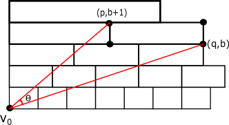
Figure 3. Angle Measurement in Preferred Sheet of $BS(2,3)$

Representing that angle by $\theta$, we have the formula.

$$\theta=\tan^{-1}\left(\frac{b+1}{p}\right)-\tan^{-1}\left(\frac{b}{q}\right)$$

and by application of a few inverse tangent identities:

$$\theta =\tan^{-1}\left(\frac{b+1}{p}\right)+\tan^{-1}\left(\frac{-b}{q}\right)$$

$$=\tan^{-1}\left(\frac{\frac{b+1}{p}+\frac{-b}{q}}{1-\frac{-b(b+1)}{pq}}\right).$$

By algebraic manipulation we then obtain:

$$\theta =\tan^{-1}\left(\frac{(b+1)q-bp}{pq+b^{2}+b}\right)$$

$$=\tan^{-1}\left(\frac{b(q-p)+q}{pq+b^{2}+b}\right)$$

$$=\tan^{-1}\left(\frac{b(q-p)}{pq+b^{2}+b}+\frac{q}{pq+b^{2}+b}\right)$$

Next we analyze this formula when $a$ and/or $b$ get large. Recall that $p$ and $q$ are both defined in terms of $a$ and $b$. In particular as one of $a$ and $b$ or both get large, $p$ and $q$ get large. Thus, the second term in the above sum clearly gets small as $a$ or $b$ get large. So, to deduce that $\theta$ approaches $0$ as$\sqrt{a^{2}+b^{2}}$ gets large, we need only check that the first term in that sum goes to zero.

We direct our attention to proving that the term

(#) $$\frac{b(q-p)}{pq+b^{2}+b}$$

approaches $0$ as $\sqrt{a^{2}+b^{2}}$ tends to infinity.

Recall that

$$b(q-p) =b(\log(\log((a+1)\left(\frac{n}{m}\right)^{b}+e))-\log(\log(a\left(\frac{n}{m}\right)^{b}+e)))$$

$$=b\log\left(\frac{\log((a+1)\left(\frac{n}{m}\right)^{b}+e)}{\log(a\left(\frac{n}{m}\right)^{b}+e)}\right)$$

We split our analysis into four cases, applying L’Hôpital’s Rule when appropriate. For simplicity of notation, we assume $m>0$; if not, replace $m$ by $|m|$ in the calculations below:

Case 1: $b$ is bounded and $a$ gets large.

$$\lim_{a\rightarrow\infty}\frac{\log\left((a+1)\left(\frac{n}{m}\right)^{b}+e\right)}{\log\left(a\left(\frac{n}{m}\right)^{b}+e\right)}=\lim_{a\rightarrow\infty}\frac{\left(\frac{n}{m}\right)^{b}}{(a+1)\left(\frac{n}{m}\right)^{b}+e}\cdot\frac{a\left(\frac{n}{m}\right)^{b}+e}{\left(\frac{n}{m}\right)^{b}}=1$$

Thus,

$$b\log\left(\frac{\log\left((a+1)\left(\frac{n}{m}\right)^{b}+e\right)}{\log\left(a\left(\frac{n}{m}\right)^{b}+e\right)}\right)\rightarrow 0$$

Case 2: $a=0$ and $b$ gets large.

$$b\log\left(\log\left(\left(\frac{n}{m}\right)^{b}+e\right)\right)$$

$$\sim b\log\left(b\right)$$

and since there is a $b^{2}$ term in the denominator, (# ‣ 3.4) approaches $0$, as desired.

Case 3: $a$ is bounded and $b$ gets large.

Then

$$\lim_{b\rightarrow\infty}\frac{\log\left((a+1)\left(\frac{n}{m}\right)^{b}+e\right)}{\log\left(a\left(\frac{n}{m}\right)^{b}+e\right)} =\lim_{b\rightarrow\infty}\frac{(a+1)\left(\frac{n}{m}\right)^{b}\log\left(\frac{n}{m}\right)}{(a+1)\left(\frac{n}{m}\right)^{b}+e}\cdot\frac{a\left(\frac{n}{m}\right)^{b}+e}{a\left(\frac{n}{m}\right)^{b}\log\left(\frac{n}{m}\right)}$$

$$=\lim_{b\rightarrow\infty}\frac{(a+1)\left(\frac{n}{m}\right)^{b}\log\left(\frac{n}{m}\right)}{a\left(\frac{n}{m}\right)^{b}\log\left(\frac{n}{m}\right)}\cdot\frac{a\left(\frac{n}{m}\right)^{b}+e}{(a+1)\left(\frac{n}{m}\right)^{b}+e}$$

$$=\frac{a+1}{a}\cdot\frac{a}{a+1}$$

$$=1$$

So

$$\log\left(\frac{\log\left((a+1)\left(\frac{n}{m}\right)^{b}+e\right)}{\log\left(a\left(\frac{n}{m}\right)^{b}+e\right)}\right)\rightarrow 0$$

and hence,

$$b\log\left(\frac{\log\left((a+1)\left(\frac{n}{m}\right)^{b}+e\right)}{\log\left(a\left(\frac{n}{m}\right)^{b}+e\right)}\right)$$

grows slower than $b$. It follows easily that (# ‣ 3.4) again approaches $0$.

Case 4: $a$ and $b$ both get large.

First notice that

$$\frac{\log\left((a+1)\left(\frac{n}{m}\right)^{b}+e\right)}{\log\left(a\left(\frac{n}{m}\right)^{b}+e\right)}\leq\frac{\log\left(2a\left(\frac{n}{m}\right)^{b}+e\right)}{\log\left(a\left(\frac{n}{m}\right)^{b}+e\right)}$$

Set $x=a\left(\frac{n}{m}\right)^{b}$. Then as $a,b\rightarrow\infty$, $x\rightarrow\infty$, hence:

$$\lim_{a,b\rightarrow\infty}\frac{\log\left(2a\left(\frac{n}{m}\right)^{b}+e\right)}{\log\left(a\left(\frac{n}{m}\right)^{b}+e\right)}=\lim_{x\rightarrow\infty}\frac{\log\left(2x+e\right)}{\log(x+e)}=\lim_{x\rightarrow\infty}\frac{2}{2x+e}\cdot\frac{x+e}{1}=1$$

And thus,

$$b\log\left(\frac{\log\left((a+1)\left(\frac{n}{m}\right)^{b}+e\right)}{\log\left(a\left(\frac{n}{m}\right)^{b}+e\right)}\right)$$

grows no faster than $b$. Again, we conclude that (# ‣ 3.4) approaches $0$.

∎

Now suppose $\overline{g}\overline{R}_{0}$ is an arbitrary tile of $\mathbb{R}\times T\left(\left|m\right|,n\right)$. We may choose an edge ray $\rho$ in $T\left(\left|m\right|,n\right)$ emanating from $\nu_{0}$ so that $\overline{g}\overline{R}_{0}$ lies in the sheet $\mathbb{R}\times\rho$, which inherits the geometry of a Euclidean half-plane with $\mathbf{v}_{0}$ at the origin. For points $\mathbf{w}_{1},\mathbf{w}_{2}\in\overline{g}\overline{R}_{0}$ we can measure the angle between segments $\overline{\mathbf{v}_{0}\mathbf{w}_{1}}$ and $\overline{\mathbf{v}_{0}\mathbf{w}_{2}}$ in this half-plane. That measure does not depend on the sheet chosen.

Corollary 3.4.

For each $\epsilon>0$, there exists $N_{\epsilon}>0$ such that if $\overline{g}\overline{R}_{0}$ is a $\overline{BS(m,n)}$-tile of $\mathbb{R}\times T\left(\left|m\right|,n\right)$ lying outside the closed $N_{\epsilon}$-ball of $\mathbb{R}\times T\left(\left|m\right|,n\right)$ centered at $\mathbf{v}_{0}$, and if $\mathbf{w}_{1},\mathbf{w}_{2}\in\overline{g}\overline{R}_{0}$, then the angle between segments $\overline{\mathbf{v}_{0}\mathbf{w}_{1}}$ and $\overline{\mathbf{v}_{0}\mathbf{w}_{2}}$ is less than $\epsilon$.

Proof.

Let $\epsilon>0$ be fixed, and apply Lemma 3.3 to obtain $M_{\epsilon/2}$ so large that if $\overline{g}\overline{R}_{0}$ is a $\overline{BS(m,n)}$-tile in the preferred positive sheet $\mathbb{R}\times\tau^{+}$ and lying outside the closed $M_{\epsilon/2}$-ball of $\mathbb{R}\times T\left(\left|m\right|,n\right)$ centered at $\mathbf{v}_{0}$, and if $\mathbf{w}_{1},\mathbf{w}_{2}\in\overline{g}\overline{R}_{0}$, then the angle between $\overline{\mathbf{v}_{0}\mathbf{w}_{1}}$ and $\overline{\mathbf{v}_{0}\mathbf{w}_{2}}$ is less than $\epsilon/2$. Then let $N_{\epsilon}=M_{\epsilon/2}+R$, where $R>0$ is chosen so large that every $\overline{BS(m,n)}$-tile that intersects $B\left(\mathbf{v}_{0},M_{\epsilon/2}\right)$ is contained in $B\left(\mathbf{v}_{0},M_{\epsilon/2}+R\right)$.

Now let $\overline{g}\overline{R}_{0}$ be an arbitrary $\overline{BS(m,n)}$-tile and $\mathbb{R}\times\rho$ a sheet of $T\left(\left|m\right|,n\right)$ containing $\overline{g}\overline{R}_{0}$.

Case 1: $\mathbb{R}\times\rho$ is a positive sheet.

In the case of the standard tiling of $\mathbb{R}\times T\left(\left|m\right|,n\right)$ (by exponentially growing rectangles) we observed that the standard tiling of $\mathbb{R}\times\rho$ is identical up to horizontal translation to that of $\mathbb{R}\times\tau^{+}$. So if the standardly tiled template of $\mathbb{R}\times\tau^{+}$ were superimposed on $\mathbb{R}\times\rho$, each tile of $\mathbb{R}\times\rho$ would be contained in a pair of side-by-side tiles of $\mathbb{R}\times\tau^{+}$. This remains true after conjugating the action by $f$. Therefore the tile $\overline{g}\overline{R}_{0}$ fits within a pair of side-by-side $\overline{BS\left(m,n\right)}$-tiles of $\mathbb{R}\times\tau^{+}$ superimposed upon $\mathbb{R}\times\rho$. So by the triangle inequality for angle measure and the choice of $N_{\epsilon}$, the angle between $\overline{\mathbf{v}_{0}\mathbf{w}_{1}}$ and $\overline{\mathbf{v}_{0}\mathbf{w}_{2}}$ is less than $\epsilon$, provided $\overline{g}\overline{R}_{0}$ lies outside the closed $N_{\epsilon}$-ball.

Case 2: $\mathbb{R}\times\rho$ is arbitrary.

As noted previously, the standard tiling of an arbitrary sheet of $\mathbb{R}\times T\left(\left|m\right|,n\right)$ refines the standard tiling of an appropriately chosen positive sheet. The same then is true for the $\overline{BS(m,n)}$-tiling. Hence, the general case can be deduced from Case 1. ∎

Theorem 3.5.

The $\overline{BS(m,n)}$-action on $\mathbb{R}\times T\left(\left|m\right|,n\right)$, together with the visual compactification $\overline{\mathbb{R}\times T\left(\left|m\right|,n\right)}$ of $\mathbb{R}\times T\left(\left|m\right|,n\right)$ with the $\ell^{2}$ metric, is a $\mathcal{Z}$-structure for $BS\left(m,n\right)$.

Proof.

We need only verify the nullity condition of Definition 2.5. Toward that end let $\mathcal{U}$ be an open cover of $\overline{\mathbb{R}\times T\left(\left|m\right|,n\right)}$, and apply Lemma 2.3 to obtain a $\delta>0$ with the property that every basic open subset of $\overline{\mathbb{R}\times T\left(\left|m\right|,n\right)}$ of the form $U\left(z,1/\delta,\delta\right)$, with $z\in\partial_{\infty}(\mathbb{R}\times T\left(\left|m\right|,n\right))$, is contained in some element of $\mathcal{U}$. By Lemma 2.7 and properness of the action, it then suffices to find $N>0$ so that every $\overline{BS(m,n)}$-translate $\overline{g}\overline{R}_{0}$ of $\overline{R}_{0}$ which lies outside $\overline{B\left(\mathbf{v}_{0},N\right)}$ is contained in $U\left(z,\frac{1}{\delta},\delta\right)$ for some $z\in\partial_{\infty}(\mathbb{R}\times T\left(\left|m\right|,n\right))$.

Suppose $\overline{g}\overline{R}_{0}$ lies outside $\overline{B\left(\mathbf{v}_{0},N\right)}$, where $N$ is yet to be specified. Choose a sheet $\mathbb{R}\times\rho$ containing $\overline{g}\overline{R}_{0}$ and a point $\mathbf{w}_{0}\mathbf{\in}\overline{g}\overline{R}_{0}$. The Euclidean ray $\overrightarrow{\mathbf{v}_{0}\mathbf{w}_{0}}$ in $\mathbb{R}\times\rho$ is an element of $\partial_{\infty}(\mathbb{R}\times T\left(\left|m\right|,n\right))$; call it $z$. Its projection onto the $\left(1/\delta\right)$-sphere of $\mathbb{R}\times T\left(\left|m\right|,n\right)$ is the point $z\left(1/\delta\right)$ where the ray $\overrightarrow{\mathbf{v}_{0}\mathbf{w}}$ intersects the semicircle of radius $1/\delta$ in $\mathbb{R}\times\rho$. For any other point $\mathbf{w\in}\overline{g}\overline{R}_{0}$ let $p_{1/\delta}\left(\mathbf{w}\right)$ denote the projection onto the $\left(1/\delta\right)$-sphere. By the law of cosines, the distance between $p_{1/\delta}\left(\mathbf{w}\right)$ and $z\left(1/\delta\right)$ is $\sqrt{(2/\delta^{2})\left(1-\cos\left(\angle\mathbf{w}_{0}\mathbf{v}_{0}\mathbf{w}\right)\right)}$. Since $\delta$ is constant, this distance can be made arbitrarily small (in particular $<\delta$), by forcing $\angle\mathbf{w}_{0}\mathbf{v}_{0}\mathbf{w}$ to be small. By Corollary 3.4, this can be arranged by making $N$ sufficiently large. Lastly, one should be sure to choose $N>1/\delta$. ∎

Corollary 3.6.

Every generalized Baumslag-Solitar group admits a $\mathcal{Z}$-structure.

Proof.

This argument was provided in Section 3.1. ∎

4. $\mathcal{EZ}$-Structures on Baumslag-Solitar Groups

We complete the proof of Theorem 1.2 by showing that the $\overline{BS(m,n)}$-action on $\mathbb{R}\times T\left(\left|m\right|,n\right))$ extends to the visual compactification $\overline{\mathbb{R}\times T\left(\left|m\right|,n\right))}$. Since this action is not by isometries and, more specifically, this action does not send rays to rays, this observation is not immediate.

Note that, since $T\left(\left|m\right|,n\right)$ is a Bass-Serre tree for $BS\left(m,n\right)$, there is a natural action by isometries of $BS\left(m,n\right)$ on $T\left(\left|m\right|,n\right))$. As such, this action extends to the visual compactification of $T\left(\left|m\right|,n\right))$ (which is just its end-point compactification) in the obvious way. As noted previously, $\partial_{\infty}(\mathbb{R}\times T\left(\left|m\right|,n\right))$ is the suspension $S^{0}\ast\partial_{\infty}T\left(\left|m\right|,n\right)$, which we may parameterize as the quotient space $[0,\pi]\times\partial_{\infty}T\left(\left|m\right|,n\right)/\sim$. Here the equivalence relation identifies the sets $\left\{0\right\}\times\partial_{\infty}T\left(\left|m\right|,n\right)$ and $\left\{\pi\right\}\times\partial_{\infty}T\left(\left|m\right|,n\right)$ to the right- and left-hand suspension points, which we denote $\mathbf{R}$ and $\mathbf{L}$. Each edge path ray $\rho$ in $T\left(\left|m\right|,n\right)$ emanating from $v_{0}$ uniquely determines both a point of $\partial_{\infty}T\left(\left|m\right|,n\right)$ and a sheet $\mathbb{R}\times\rho\subseteq\mathbb{R}\times T\left(\left|m\right|,n\right))$. The great semicircle $C_{\rho}$ of rays in $\mathbb{R}\times\rho$ based at $\mathbf{v}_{0}$ (parameterized by the angles they make with the positive $x$-axis), trace out the set $[0,\pi]\times\{\rho\}\subseteq S^{0}\ast\partial_{\infty}T\left(\left|m\right|,n\right)$.

Given a homeomorphism $h:\partial_{\infty}T\left(\left|m\right|,n\right)\rightarrow\partial_{\infty}T\left(\left|m\right|,n\right)$, the suspension of $h$ is the homeomorphism of $S^{0}\ast\partial_{\infty}T\left(\left|m\right|,n\right)$ which fixes $\mathbf{R}$ and $\mathbf{L}$ and takes each great semicircle $C_{\rho}$ to $C_{h\left(\rho\right)}$ in a parameter-preserving manner. The reflected suspension of $h$ switches $\mathbf{R}$ and $\mathbf{L}$ and takes the point on $C_{\rho}$ with parameter $\theta$ to the point on $C_{h\left(\rho\right)}$ with parameter $\pi-\theta$. We will complete the proof of Theorem 1.2 for cases $m>0$, by proving the following proposition.

Proposition 4.1.

For $m>0$, the suspension of the $BS(m,n)$-action on $\partial_{\infty}T\left(\left|m\right|,n\right)$ extends the $\overline{BS(m,n)}$-action on $\mathbb{R}\times T\left(\left|m\right|,n\right))$.

Remark 1.

Cases where $m<0$ require the use of reflected suspensions; we will handle those cases after completing Proposition 4.1.

Proof of Proposition 4.1 requires some additional terminology and notation. Thus far we have understood the space $\mathbb{R}\times T\left(\left|m\right|,n\right))$ as a union of sheets, each with a common origin $\mathbf{v}_{0}=\left(0,v_{0}\right)$ and a common “edge”, $\mathbb{R}\times\left\{v_{0}\right\}$. As such, each sheet has a natural system of Euclidean local coordinates, where a point $\left(x,y\right)\in\mathbb{R}\times\rho$ is represented by the pair of real numbers $\left(x,d\right)$, where $d$ is the distance along $\rho$ from $v_{0}$ to $y$.

Since the actions of $B\left(m,n\right)$ on $\mathbb{R}\times T\left(\left|m\right|,n\right))$ (standard and conjugated) do not send sheets to sheets, it is useful to expand our perspective slightly. If $\sigma$ is an arbitrary edge path ray in $T\left(\left|m\right|,n\right)$ emanating from a vertex $v$, then $\mathbb{R}\times\sigma$ is again convex and isometric to a Euclidean half-plane. Call $\mathbb{R}\times\sigma$ a generalized sheet and attach to it the obvious system of Euclidean local coordinates, where $\mathbf{v=}\left(0,v\right)$ plays the role of the origin. Note that:

• if $v_{0}$ lies on $\sigma$, then $\mathbb{R}\times\sigma$ contains the sheet $\mathbb{R}\times\sigma^{\prime}$ where $\sigma^{\prime}\subseteq\sigma$ is the subray beginning at $v_{0}$; and

• if $v_{0}\notin\sigma$, there is an edge path ray $\sigma^{\prime}$ emanating from $v_{0}$ and containing $\sigma$ as a subray, in which case the sheet $\mathbb{R}\times\sigma^{\prime}$ contains $\mathbb{R}\times\sigma$.

In each of the above cases, the edges of half-planes $\mathbb{R}\times\sigma$ and $\mathbb{R}\times\sigma^{\prime}$ cobound a Euclidean strip in the larger of the two sets. As a result, a ray in $\mathbb{R}\times\sigma$ emanating from an arbitrary edge point $\left(x,v\right)$ at an angle $\theta$ with $[x,\infty)\times\left\{v\right\}$ is asymptotic in $\mathbb{R}\times T\left(\left|m\right|,n\right))$ to the ray in $\mathbb{R}\times\sigma^{\prime}$ emanating from $\mathbf{v}_{0}$ and forming the same angle with $[0,\infty)\times v_{0}$. As such both rays represent the same element of $S^{0}\ast\partial_{\infty}T\left(m,n\right)$, the point on the the semicircle $C_{\sigma^{\prime}}$ with parameter $\theta$.

Proof of Proposition 4.1 .

In this proof we allow $s$ and $t$ to represent the isometries generating the action of $BS(m,n)$ on the Bass-Serre tree $T\left(\left|m\right|,n\right))$ as well as the extensions of those isometries to the visual compactification of $T\left(\left|m\right|,n\right))$. We use the same symbols to denote the homeomorphisms generating the standard $BS\left(m,n\right)$-action on $\mathbb{R}\times T\left(\left|m\right|,n\right))$, as described in Section 3.2. It will be useful to have formulaic representations of these functions.

As an isometry of $T\left(\left|m\right|,n\right))$, $s$ fixes $v_{0}$, but permutes the collection of rays emanating from that vertex. As a self-homeomorphism of $\mathbb{R}\times T\left(\left|m\right|,n\right))$, the action of $s$ on the $\mathbb{R}$-coordinate is translation by $1/n$. So, if $\mathbb{R}\times\rho$ is an arbitrary sheet and $\rho^{\prime}$ is the image of $\rho$ under $s$ in the Bass-Serre tree, then, as a homeomorphism of $\mathbb{R}\times T\left(\left|m\right|,n\right))$, $s$ takes points of $\mathbb{R}\times\rho$ with local coordinates $\left(x,d\right)$ to points of $\mathbb{R}\times\rho^{\prime}$ with local coordinates $\left(x+\frac{1}{n},d\right)$.

As an isometry of $T\left(\left|m\right|,n\right))$, $t$ sends $v_{0}$ to a vertex $v_{1}$, one unit away; and as a self-homeomorphism of $\mathbb{R}\times T\left(\left|m\right|,n\right))$, the action of $t$ on the $\mathbb{R}$-coordinate is multiplication by $n/m$. So, if $\mathbb{R}\times\rho$ is an arbitrary sheet and $\rho^{\prime}$ is its image under $t$ in the Bass-Serre tree, $s$ takes points of $\mathbb{R}\times\rho$ with local coordinates $\left(x,d\right)$ to points of $\mathbb{R}\times\rho^{\prime}$ with local coordinates $\left(\left(\frac{n}{m}\right)x,d\right)$.

Now consider the homeomorphisms $\overline{s}=f\circ s\circ f^{-1}$ and $\overline{t}=f\circ t\circ f^{-1}$ which generate the $\overline{B\left(m,n\right)}$-action on $\mathbb{R}\times T\left(\left|m\right|,n\right))$. Since the suspension of a composition is the composition of the suspensions, it is enough to verify the proposition for these two elements. Recall that $f$ and $f^{-1}$ are given by the formulas

$$\left(x,y\right)\overset{f}{\longrightarrow}\left(\operatorname{sgn}\left(x\right)\log\left(\log\left(\left|x\right|+e\right)\right),y\right)\text{,\hskip 10.84006ptand}$$

$$\left(x,y\right)\overset{f^{-1}}{\longrightarrow}\left(\operatorname{sgn}\left(x\right)(\exp\left(\exp\left(\left|x\right|\right)\right)-e\right),y)$$

Let $\mathbb{R}\times\rho$ be an arbitrary sheet, and for $p,q\in\mathbb{Z}$ with $p\geq 0$, let $\overrightarrow{\mathbf{r}_{\frac{p}{q}}}=\left\{\left(qx,px\right)\mid x\in\mathbb{R}^{+}\right\}$, i.e., $\overrightarrow{\mathbf{r}_{\frac{p}{q}}}$ is the ray in $\mathbb{R}\times\rho$ with slope $p/q$. If $\rho^{\prime}$ is the image of $\rho$ under $s$ in the Bass-Serre tree, then $\overline{s}$ takes $\mathbb{R}\times\rho$ onto $\mathbb{R}\times\rho^{\prime}$ and the image of $\overrightarrow{\mathbf{r}_{\frac{p}{q}}}$ is the set of points with local coordinates

(4.1) $$\{(\delta_{q,x,n}\cdot\log(\log(\exp\left(\exp\left(\left|q\right|x\right)\right)+\frac{1}{n})),px)\mid x\in\mathbb{R}^{+}\},$$

where $\delta_{q,x,n}=\pm 1$ is a small variation on $\operatorname{sgn}\left(q\right)$. Specifically,

$$\delta_{q,x,n}=\operatorname{sgn}(\operatorname{sgn}\left(q\right)\log(\log(x+e))+\frac{1}{n})$$

which is identical to $\operatorname{sgn}\left(q\right)$ except when $\log\left(\log\left(x+e\right)\right)<\frac{1}{n}$ and $q<0$. Most importantly, the image of $\overrightarrow{\mathbf{r}_{\frac{p}{q}}}$ under $\overline{s}$ is a topologically embedded (non-geodesic) ray in $\mathbb{R}\times\rho^{\prime}$ which, in local coordinates, emanates from $\left(\log\log\left(e+\frac{1}{n}\right),0\right)$ and is asymptotic to geodesic rays in $\mathbb{R}\times\rho^{\prime}$ with slope $p/q$. That is easily seen by letting $x$ approach infinity in formula (4.1). From this it can be seen that the restriction of $\overline{s}$ taking $\mathbb{R}\times\rho$ onto $\mathbb{R}\times\rho^{\prime}$ extends to the visual boundaries of these half-planes by taking $C_{\rho}$ onto $C_{\rho^{\prime}}$ in a parameter preserving manner. Since this is true for each sheet, it follows that the suspension of the homeomorphism $s:\partial_{\infty}T\left(\left|m\right|,n\right)\rightarrow\partial_{\infty}T\left(\left|m\right|,n\right)$ extends $\overline{s}:\mathbb{R}\times T\left(\left|m\right|,n\right))\rightarrow\mathbb{R}\times T\left(\left|m\right|,n\right))$ over the visual boundary.

Next consider the homeomorphism $\overline{t}$. Again let $\overrightarrow{\mathbf{r}_{\frac{p}{q}}}$ be a ray (as described above) in an arbitrary sheet $\mathbb{R}\times\rho$ and let $\rho^{\prime}$ be the $t$-image of $\rho$ under the action on $T\left(\left|m\right|,n\right)$. In local coordinates, the image of $\overrightarrow{\mathbf{r}_{\frac{p}{q}}}$ is the set of points in $\mathbb{R}\times\rho^{\prime}$ with local coordinates

$$\{(\operatorname{sgn}\left(q\right)\log\left(\log\left(\frac{n}{m}\exp\left(\exp\left(\left|q\right|x\right)\right)+(\frac{m-n}{m})\cdot e\right)\right),px)\mid x\in\mathbb{R}^{+}\}.$$

Consider now the ratios of the coordinates of these points as $x$ gets large, i.e.,

$$\operatorname{sgn}\left(q\right)\cdot\lim_{x\rightarrow\infty}\frac{px}{\log\left(\log\left(\frac{n}{m}\exp\left(\exp\left(\left|q\right|x\right)\right)+(\frac{m-n}{m})\cdot e\right)\right)}$$

By another elementary but messy calculation involving L’Hôpital’s Rule, this limit is $p/q$. As such, the image of $\overrightarrow{\mathbf{r}_{\frac{p}{q}}}$ under $\overline{t}$ is a topologically embedded (non-geodesic) ray in $\mathbb{R}\times\rho^{\prime}$ emanating (in local coordinates) from $\left(0,0\right)$ and asymptotic to rays in $\mathbb{R}\times\rho^{\prime}$ with slope $p/q$. As before, the restriction of $\overline{t}$ taking $\mathbb{R}\times\rho$ onto $\mathbb{R}\times\rho^{\prime}$ extends to the visual boundaries of these half-planes by taking $C_{\rho}$ onto $C_{\rho^{\prime}}$ in a parameter preserving manner. And since this is true for all sheets, the suspension of $t:\partial_{\infty}T\left(\left|m\right|,n\right)\rightarrow\partial_{\infty}T\left(\left|m\right|,n\right)$ extends $\overline{t}:\mathbb{R}\times T\left(\left|m\right|,n\right))\rightarrow\mathbb{R}\times T\left(\left|m\right|,n\right))$ over the visual boundary. ∎

To complete Theorem 1.2, we need an analog of Proposition 4.1 for $m<0$. In those cases, we cannot simply suspend the $BS\left(m,n\right)$-action on $\partial_{\infty}T\left(\left|m\right|,n\right)$ to get the appropriate extension of the $\overline{BS(m,n)}$-action on $\mathbb{R}\times T\left(\left|m\right|,n\right))$. That is because homeomorphisms $t$ and $\overline{t}$ now flip the orientation of the $\mathbb{R}$-factor. More precisely, if $r:\mathbb{R}\times T\left(\left|m\right|,n\right))\rightarrow\mathbb{R}\times T\left(\left|m\right|,n\right))$ is the reflection homeomorphism taking $\left(x,y\right)$ to $\left(-x,y\right)$, then $t$ and $\overline{t}$ are the homeomorphisms $r\circ t^{\prime}$ and $r\circ\overline{t^{\prime}}$, where $t^{\prime}$ and $\overline{t^{\prime}}$ are the homeomorphisms studied earlier in cases where $m>0$. Obviously, if $\overline{t^{\prime}}$ extends to the visual boundary of $\mathbb{R}\times T\left(\left|m\right|,n\right))$ by suspending the corresponding homeomorphism of $\partial_{\infty}T\left(\left|m\right|,n\right))$, then $\overline{t}$ extends to the visual boundary of $\mathbb{R}\times T\left(\left|m\right|,n\right))$ via the reflected suspension of that same homeomorphism. By contrast, the homeomorphisms $s$ and $\overline{s}$ are no different when $m<0$ than they are when $m>0$.

For $m<0$ define $\phi:BS\left(m,n\right)\rightarrow\mathbb{Z}$ to be the quotient map obtained by modding out by the normal closure of the subgroup $\left\langle s\right\rangle$. Then, for an action of $BS\left(m,n\right)$ on $\partial_{\infty}T\left(\left|m\right|,n\right))$, define the corresponding $t$-reflected action of $BS\left(m,n\right)$ on $S^{0}\ast\partial_{\infty}T\left(\left|m\right|,n\right))$ as follows:

• if $\phi\left(g\right)$ is even, then $g:S^{0}\ast\partial_{\infty}T\left(\left|m\right|,n\right))\rightarrow S^{0}\ast\partial_{\infty}T\left(\left|m\right|,n\right))$ is the suspension of $g:\partial_{\infty}T\left(\left|m\right|,n\right))\rightarrow\partial_{\infty}T\left(\left|m\right|,n\right))$, and

• if $\phi\left(g\right)$ is odd, then $g:S^{0}\ast\partial_{\infty}T\left(\left|m\right|,n\right))\rightarrow S^{0}\ast\partial_{\infty}T\left(\left|m\right|,n\right))$ is the reflected suspension of $g:\partial_{\infty}T\left(\left|m\right|,n\right))\rightarrow\partial_{\infty}T\left(\left|m\right|,n\right))$.

Proof of the following is now essentially the same as Proposition 4.1.

Proposition 4.2.

For $m<0$, the $t$-reflected suspension of the $BS(m,n)$-action on $\partial_{\infty}T\left(\left|m\right|,n\right)$ extends the $\overline{BS(m,n)}$-action on $\mathbb{R}\times T\left(\left|m\right|,n\right))$.

Remark 2.

The argument by which $\mathcal{Z}$-structures for generalized Baumslag-Solitar groups were obtained from the existence of $\mathcal{Z}$-structures on ordinary Baumslag-Solitar groups does not extend to $\mathcal{EZ}$-structures. That is because equivariance can be lost when applying Proposition 2.8. We leave the issue of $\mathcal{EZ}$-structures for generalized Baumslag-Solitar groups for later.

References

- [AMN11] H. Abels, A. Manoussos, and G. Noskov, Proper actions and proper invariant metrics, J. Lond. Math. Soc. (2) 83 (2011), no. 3, 619–636. MR 2802502
- [Bes96] Mladen Bestvina, Local homology properties of boundaries of groups, Michigan Math. J. 43 (1996), no. 1, 123–139. MR 1381603
- [BH99] M. Bridson and A. Haefliger, Metric spaces of non-positive curvature, Grundlehren der Mathematischen Wissenschaften [Fundamental Principles of Mathematical Sciences], vol. 319, Springer-Verlag, Berlin, 1999.
- [BM91] Mladen Bestvina and Geoffrey Mess, The boundary of negatively curved groups, J. Amer. Math. Soc. 4 (1991), no. 3, 469–481. MR 1096169
- [Dah03] F. Dahmani, Classifying spaces and boundaries for relatively hyperbolic groups, Proc. London Math Soc. 86 (2003), no. 3, 666–684.
- [Dra06] A. Dranishnikov, On Bestvina-Mess formula, Contemporary Mathematics 394 (2006), no. 1, 77 –85.
- [FL05] F. T. Farrell and J.-F. Lafont, EZ-structures and topological applications, Comment. Math. Helv. 80 (2005), no. 1, 103–121. MR 2130569
- [Ger92] S. M. Gersten, Dehn functions and -norms of finite presentations, Algorithms and classification in combinatorial group theory (Berkeley, CA, 1989), Math. Sci. Res. Inst. Publ., vol. 23, Springer, New York, 1992, pp. 195–224. MR 1230635
- [GM18] Craig R. Guilbault and Molly A. Moran, Proper homotopy types and z-boundaries of spaces admitting geometric group actions, Expositiones Mathematicae (2018).
- [Mar14] A. Martin, Non-positively curved complexes of groups and boundaries, Geom. Topol. 18 (2014), no. 1, 31–102.
- [OP09] D. Osajda and P. Przytycki, Boundaries of systolic groups, Geom. Topol. 13 (2009), no. 5, 2807 –2880.
- [Pie18] Brian Pietsch, Z-structures and semidirect products with an infinite cyclic group, Thesis (Ph.D.)–The University of Wisconsin - Milwaukee, 2018.
- [Tir11] C. Tirel, Z-structures on product groups, Algebr. Geom. Topol. 11 (2011), no. 5, 2587–2625.
- [Why01] K. Whyte, The large scale geometry of the higher Baumslag-Solitar groups, Geom. Funct. Anal. 11 (2001), no. 6, 1327–1343. MR 1878322