Conditional expectation of the duration of the classical gambler problem with defects

Abstract

The effect of space inhomogeneities on a diffusing particle is studied in the framework of the 1D random walk. The typical time needed by a particle to cross a one–dimensional finite lane, the so–called residence time, is computed possibly in presence of a drift. A local inhomogeneity is introduced as a single defect site with jumping probabilities differing from those at all the other regular sites of the system. We find complex behaviors in the sense that the residence time is not monotonic as a function of some parameters of the model, such as the position of the defect site. In particular we show that introducing at suitable positions a defect opposing to the motion of the particles decreases the residence time, i.e., favors the flow of faster particles. The problem we study in this paper is strictly connected to the classical gambler’s ruin problem, indeed, it can be thought as that problem in which the rules of the game are changed when the gambler’s fortune reaches a particular a priori fixed value. The problem is approached both numerically, via Monte Carlo simulations, and analytically with two different techniques yielding different representations of the exact result.

Pacs: 02.50.Ey; 02.50.-r; 05.40.Fb

Keywords: Gambler’s ruin problem, residence time, random walk, Monte Carlo methods

AMS Subject Classification: : 82B41

1 Introduction

Particles flowing across obstacles exhibit interesting effects [1]. The dynamics, depending on the details of the systems, can be either accelerated or slowed down. Anomalous diffusion, i.e., sub–linear behavior with respect to time of the mean square distance traveled by particles undergoing Brownian motion, is observed in cells and can be explained as an effect of macromolecules playing the role of obstacles for the diffusing smaller molecules [2, 3, 4, 5]. In many other different contexts it has been observed that obstacles surprisingly accelerate the dynamics. An obstacle placed close to the exit, can improve the out–coming flow in a granular system in presence of clogging [6, 7, 8, 9]. Similar phenomena are observed in pedestrian flows [10, 11, 12, 13, 14, 15] in case of panic, where clogging at the door can be reduced by means of suitably positioned obstacles [16, 17, 18, 19].

These phenomena are discussed here in the very basic scenario of the 1D symmetric random walk in connection with the behavior, as a function of the properties of the obstacle, of the typical time that a particle started at the left end of the lane needs to cross the whole lane. This time will be called residence time. Here, the obstacle is represented by a single defect site characterized by different jumping probabilities with respect to those associated with all the other regular sites. This 1D model can be also interpreted as a toy model for the 2D finite strip in which a rectangular obstacle is placed inside the strip in such a way that its right–hand boundary is in touch with the right boundary of the strip. The defect site mimics the sites in the first column of the 2D strip on the left of the obstacle, indeed, the 2D walker in such a column has a probability to move to the right smaller than the probability to move to the left. The sites on the right of the defect are regular, since when the 2D walker enters one of the two channels flanking the obstacle its probability to move to the right or to the left is no more influenced by the obstacle.

It is worth mentioning that the problem we study here shares some features with the so–called blockage problem [20, 21, 22], where one considers a 1D dynamics with a slow down bond or site. The main problem, there, is that of understanding the effect of the local slow down on the stationary current in the thermodynamics limit.

The residence time issue, as described above, has been firstly raised in [23, 24], where the flow of particles in an horizontal strip undergoing a random walk with exclusion rule has been considered [25]. One of the most interesting results investigated in those papers is the possibility to spot complex behaviors, in the sense that the residence time unexpectedly shows up to be a not monotonic function of some parameters of the obstacles. The phenomenon was interpreted there as a consequence of the hard core particle interaction that gives rise to peculiar stationary particle density profiles. On the other hand, the studies reported in [26, 27] show that, even for not interacting particles, complex residence time behaviors can be observed as purely geometric effects. In [27] the framework of Kinetic Theory was adopted and a model with particles moving according to the linear Boltzmann dynamics was studied. In [26] the simple symmetric random walk was considered both in one and two dimensions. The one–dimensional reduction of the 2D obstacle problem was constructed by considering a 1D simple symmetric random walk with two defect sites modelling the effect of the obstacle on the motion of the particles.

In this paper we consider a single defect, but we relax the symmetry assumption and consider driven random walks as well. The residence time problem we study in this paper can be rephrased in the language of the classical gambler’s ruin problem. In such a classical problem a gambler starts with initial fortune $x_{0}$ and at each time he plays his fortune is either incremented by one with probability $p$ or decreased by one with probability $q=1-p$. Fixed the goal fortune $L$, the gambler goes on playing till either his fortune becomes $L$ or he goes bankrupt, namely his fortune becomes zero. We say that the gambler wins if his fortune becomes $L$ before going bankrupt, otherwise we say that the gambler loses. The probability that the gambler reaches his target $L$ before going bankrupt, in the random walk language, is the probability that the particle started at site $x_{0}$ reaches the site $L$ before visiting the site zero. In the random walk language the residence time is the mean time needed by a particle started at site one to reach site $L$ conditioned to the fact that site $L$ is reached before the particle visits site zero. This quantity, in the gambler’s language, is the mean duration of the game for the gambler with initial fortune $1$ conditioned to the fact that the gambler wins. In the sequel we shall define the model as a random walk model, but we shall often use its gambler’s interpretation.

A classical reference for the gambler’s ruin problem is the book [28] where the winning probability is studied. In [29] the author investigates the conditioned duration (residence time). In [30] both the winning probability and the conditioned duration of the game are computed in the case $0<p+q<1$, that is to say, considering the possibility of ties. Here, in the most general case, we address and solve the winning probability and the conditioned duration of the game questions introducing a defect site, that is to say, in the gambler’s language, the winning and loosing probabilities in a particular round differ from those characterizing all the other rounds. We perform both a numerical and an exact computation of the winning probability and of the conditioned duration of the game. The exact computation is performed both using the generating function method proposed in [28, 29, 30] and the method developed in [26] to attack the problem with two defects.

Using the random walk language, we discuss the dependence of the residence time on the defect parameters both in the symmetric and asymmetric case, $p=q$ and $p\neq q$ respectively. In particular we find a complex behavior of the residence time with respect to the position of the defect, namely, we show that the residence time can be either increased or decreased, with respect to the no defect case, depending on the position of the obstacle. This effect is found both in the symmetric and in the asymmetric cases, but its magnitude is more important in the first case. In the gambler language, this means that the mean duration of the game, conditioned to the fact that the players wins, changes if the rounds played when the gambler’s fortune has an a priori fixed value are played with different rules. This is obvious, but highly not trivial is the fact that depending on the value of the fortune at which the rules are modified the duration of the game can either increase or decrease. We also stress that the dependence of the residence time on the position of the defect is not symmetric when the defect is moved along the lane, as it was remarked in [26] this could be connected with the possibility to observe uphill currents [31, 32] in presence of obstacles.

The paper is organized as follows. In Section 2 we define the model. In Section 3 we find two exact representations of the residence time. In Section 4 we compare our exact results to the Monte Carlo estimate of the residence time and we discuss our findings.

2 The model

We consider a simple random walk on $\{0,1,\dots,L\}$, i.e., the set $[0,L]\cap\mathbb{Z}$. The sites $0$ and $L$ are absorbing, so that when the particle reaches one of these two sites the walk is stopped. All the sites $1,\dots,L-1$ are regular except for the site $d$ called defect or singular site (see Figure 1), with $d\in\{2,\dots,L-2\}$. The parameter $d$ is chosen in such a way that the defect site cannot be $1$ or $L-1$. The number of regular sites on the left (resp. right) of the defect site is $d-1$ (resp. $L-d-1$).

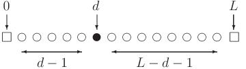
Figure 1: Representation of the lattice on which the model is defined. Open and solid circles respectively represent regular and singular (defect) sites. The two squared box represent the two boundary absorbing sites.

At each unit of time the walker jumps to a neighboring site according to the following rule: if it is on a regular site, then it performs a simple random walk with probabilities $p$ to right, $q$ to left. If $p+q<1$ the walker does not move with probability $1-p-q$. When it is at the defect site it jumps with probability $p^{\prime}$ to the right, with probability $q^{\prime}$ to the left, and with probability $\varepsilon$ it does not move. Here, $p^{\prime}\in(0,1)$ and $\varepsilon\in[0,1)$ such that $p^{\prime}+q^{\prime}+\varepsilon=1$. If $p+q=1$, $p^{\prime}=p$, and $q^{\prime}=q$ the classical gambler ruin problem is recovered [28, 29, 30].

The array $1,\dots,L-1$ will be called the lane. The sites $0$ and $L$ will be, respectively, called the left and right exit of the lane.

This 1D model can be also interpreted as a toy model for the 2D finite strip in which a rectangular obstacle of width $L-d-1$ is placed inside the strip in such a way that its right–hand boundary is in touch with the right boundary of the strip. The defect site $d$ mimics the sites in the first column of the 2D strip on the left of the obstacle. Indeed, the 2D walker in such a column has a probability to move to the right smaller since it could hit the obstacle. Let us stress that the sites $d+1,\dots,L-1$ are regular, since when the 2D walker enters one of the two channels flanking the obstacle its probability to move to the right or to the left is not influenced by the obstacle anymore. The symmetric situation of a 2D obstacle of width $d-1$ and left–hand boundary in touch with the left boundary of the strip can be considered. In this case the decreasing probability is the one to jump to the left from the column on the right of the obstacle.

The main quantity of interest is the residence time, which is defined by starting the walk at site $1$ and computing the typical time that the particle takes to reach the site $L$ conditioned to the fact that it reaches $L$ before $0$. We let $x_{t}$ be the position of the walker at time $t$ and denote by $\mathbb{P}_{k}$ and $\mathbb{E}_{k}$ the probability associated to the trajectories of the walk and the related average operator for the walk started at $x_{0}=k$ with $k=1,\dots,L-1$. We let $T_{i}$ be the first hitting time to $i$, namely, the first time at which the trajectory of the walk reaches the site $i$, with the convention that $T_{i}=\infty$ if the trajectory does not reach the site $i$. The main quantity of interest is the residence time or total residence time

$$R=\mathbb{E}_{1}[T_{L}|T_{L}<T_{0}]=\sum_{t=1}^{\infty}t\mathbb{P}_{1}[T_{L}=t|T_{L}<T_{0}]\;\;.$$ (1)

Note that the residence time is defined for the walk started at $x_{0}=1$ and the average is computed conditioning to the event $T_{L}<T_{0}$, namely, conditioning to the fact that the particle exits the lane through the right exit.

3 Exact computation of the residence time

In this section we compute the residence time (1) for the model introduced in Section 2. We first deal with the crossing probability and then with the residence time. We use standard techniques developed in [28, 29, 30] and compare the results with those obtained by applying the methods developed in [26] to tackle a similar model with two defects.

3.1 Crossing probability

For the classical gambler’s ruin problem (no defect), the probability of the gambler’s ultimate ruin with initial fortune $i$, i.e., $t_{i}=\mathbb{P}_{i}[T_{0}<T_{L}]$, is given by

$$t_{i}=\frac{(q/p)^{L}-(q/p)^{i}}{(q/p)^{L}-1}\;\textrm{ for }\;p\neq q\;\textrm{ and }\;t_{i}=1-(i/L)\;\textrm{ for }\;p=q,$$

see, for instance, [28]. In the random walk language $t_{i}$ is the probability that the walker started at site $i$ reaches the site $0$ before $L$.

Here, we generalize this result to the problem stated in Section 2, namely, for the random walk on the lane with a defect site. Starting with an initial fortune $i$, after one trial the gambler fortune is $i+1$ or $i-1$, or $i$ if it doesn’t move. It follows that

$$\begin{split}&t_{i}=pt_{i+1}+qt_{i-1}+(1-p-q)t_{i},\quad\forall i=1,\ldots,d-1,\\ &t_{d}=p^{\prime}t_{d+1}+q^{\prime}t_{d-1}+(1-p^{\prime}-q^{\prime})t_{d},\\ &t_{j}=pt_{j+1}+qt_{j-1}+(1-p-q)t_{j},\quad\forall j=d+1,\ldots,L-1.\end{split}$$ (2)

Note that since the random walk ends in $0$ or $L$ respectively with the win or the loss of the gambler, $t_{0}=1$ and $t_{L}=0$.

To solve (2), we first note that the first set of equations (2) can be straightforwardly rewritten as

$$pt_{i}-qt_{i-1}=pt_{i+1}-qt_{i}\;\textrm{ for }\;i=1,\dots,d-1.$$

Hence, we let $\sigma=pt_{i}-qt_{i-1}$ for $i=1,\ldots,d$, recall $t_{0}=1$, and, dividing by $p$, we get

$$\begin{split}&t_{1}=\frac{\sigma}{p}+\frac{q}{p},\\ &t_{2}=\frac{q}{p}t_{1}+\frac{\sigma}{p}=\Big{(}\frac{q}{p}\Big{)}^{2}+\frac{q}{p}\frac{\sigma}{p}+\frac{\sigma}{p},\\ &\qquad\vdots\\ &t_{d}=\frac{q}{p}t_{d-1}+\frac{\sigma}{p}=\Big{(}\frac{q}{p}\Big{)}^{d}+\frac{\sigma}{p}\sum_{k=0}^{d-1}\Big{(}\frac{q}{p}\Big{)}^{k}.\end{split}$$ (3)

By treating similarly the second equation in (2), we find $(p^{\prime}+q^{\prime})t_{d}=p^{\prime}t_{d+1}+q^{\prime}t_{d-1}$, so that

$$\begin{split}t_{d+1}&=-(q^{\prime}/p^{\prime})t_{d-1}+((p^{\prime}+q^{\prime})/p^{\prime})t_{d}=(q^{\prime}/p^{\prime})(t_{d}-t_{d-1})+t_{d}\\ &=\frac{q^{\prime}}{p^{\prime}}\Big{(}\frac{q}{p}\Big{)}^{d-1}\Big{(}\frac{q}{p}-1+\frac{\sigma}{p}\Big{)}+\Big{(}\frac{q}{p}\Big{)}^{d}+\frac{\sigma}{p}\sum_{k=0}^{d-1}\Big{(}\frac{q}{p}\Big{)}^{k}.\end{split}$$ (4)

The third family of equations (2) allows us to write

$$pt_{j+1}-qt_{j}=pt_{j}-qt_{j-1}=\lambda\;\textrm{ for }\;j=d+1,\ldots,L-1.$$ (5)

Using the expressions (3) and (4) of $t_{d+1}$ and $t_{d}$ we can compute the explicit expression. Then, we find the probabilities

$$\begin{split}&t_{d+2}=\frac{\lambda}{p}+\frac{q}{p}t_{d+1}\\ &t_{d+3}=\frac{\lambda}{p}+\frac{q}{p}t_{d+2}=\Big{(}\frac{q}{p}\Big{)}^{2}t_{d+1}+\frac{\lambda}{p}\Big{(}1+\frac{q}{p}\Big{)}\\ &\qquad\vdots\\ &t_{L}=\Big{(}\frac{q}{p}\Big{)}^{L-d-1}t_{d+1}+\frac{\lambda}{p}\sum_{k=0}^{L-d-2}\Big{(}\frac{q}{p}\Big{)}^{k}.\end{split}$$ (6)

Finally, using $t_{L}=0$ we can find $\sigma$. Indeed, by letting $t_{L}=0$ and $\lambda=pt_{d+1}-qt_{d}$ in the last of equations (6), after some algebra, we get

$$t_{d+1}\Big{[}\sum_{k=0}^{L-d-1}\Big{(}\frac{q}{p}\Big{)}^{k}\Big{]}-\frac{q}{p}t_{d}\Big{[}\sum_{k=0}^{L-d-2}\Big{(}\frac{q}{p}\Big{)}^{k}\Big{]}=0.$$ (7)

To complete the computation we have to distinguish the two cases $p\neq q$ and $p=q$. The second one is easier and will be treated later.

Case $p\neq q$. Equation (7) can be re written as

$$\frac{1-(q/p)^{L-d}}{1-q/p}t_{d+1}-\frac{q/p-(q/p)^{L-d}}{1-q/p}t_{d}=0.$$

Thus, multiplying by $1-(q/p)$ and using the explicit expressions of $t_{d+1}$ and $t_{d}$, after some algebra we get the expression of $\sigma$:

$$\begin{split}{\sigma}&=p\Big{\{}\Big{[}\Big{(}\frac{q}{p}\Big{)}^{L-d}-1\Big{]}\Big{[}\frac{q^{\prime}}{p^{\prime}}\Big{(}\frac{q}{p}\Big{)}^{d-1}\Big{(}\frac{q}{p}-1\Big{)}+\Big{(}\frac{q}{p}\Big{)}^{d}\Big{]}+\Big{(}\frac{q}{p}\Big{)}^{d+1}-\Big{(}\frac{q}{p}\Big{)}^{L}\Big{\}}\\ &\phantom{=}\times\Big{\{}\Big{[}1-\Big{(}\frac{q}{p}\Big{)}^{L-d}\Big{]}\Big{[}\frac{q^{\prime}}{p^{\prime}}\Big{(}\frac{q}{p}\Big{)}^{d-1}+\frac{1-(q/p)^{d}}{1-q/p)}\Big{]}+\Big{[}\Big{(}\frac{q}{p}\Big{)}^{L-d}-\frac{q}{p}\Big{]}\frac{1-(q/p)^{d}}{1-q/p}\Big{\}}^{-1}\end{split}$$ (8)

Once $\sigma$ is known, we can write explicitly each $t_{i}$. In particular we can write the probability $t_{1}=\mathbb{P}_{1}[T_{0}<T_{L}]$ that the particle started at $1$ exits the lane in $0$ and the probability $1-t_{1}=1-\mathbb{P}_{1}[T_{0}<T_{L}]$ that the particle started at $1$ exits the lane in $L$. Recalling that $t_{1}=\sigma/p+q/p$, some painful algebra yields

$$1-t_{1}=\frac{p^{\prime}(p-q)q}{p(-p^{\prime}q(-1+(q/p)^{d})+pq^{\prime}(-(q/p)^{L}+(q/p)^{d}))}.$$ (9)

Note that the result does not change if at the regular sites the probabilities to jump right $p_{i}$, to jump left $q_{i}$ or to stay $r_{i}$ are not constant anymore, but the ratio $p_{i}/q_{i}=p/q$ is conserved. Indeed, the equation on a generic site becomes

$$t_{i}=(p_{i}+q_{i}+r_{i})t_{i}=p_{i}t_{i+1}+q_{i}t_{i-1}+r_{i}t_{i}$$

so that (3)–(8) are still valid.

We remark that the probability $1-t_{1}$ can be also calculated by means of the Markov property following the ideas developed in [26]. Let us define

$$p_{1}=\mathbb{P}_{1}(T_{d}<T_{0}),\;p_{2}=\mathbb{P}_{d}(T_{d+1}<T_{0}),\;\textrm{ and }\;p_{3}=\mathbb{P}_{d+1}(T_{L}<T_{0}).$$

By using the classical gambler’s ruin problem results we find $p_{1}=({1-(q/p)})({1-(q/p)^{d}})^{-1}$. We observe that a random walk starting from the site $1$ reaches again the site $d$ before hitting $d+1$ for the first time with probability $(1-p^{\prime}-q^{\prime})+(q^{\prime}(1-(q/p)^{d-1})(1-(q/p)^{d})^{-1})$, where the second term in the sum is due to trajectories that reach $d-1$ after one step and than eventually again $d$ with probability $(1-(q/p)^{d-1})(1-(q/p)^{d})^{-1}$. So the probability $p_{2}$ reads

$$p_{2}=\sum_{k=0}^{+\infty}p^{\prime}[(1-p^{\prime}-q^{\prime})+(q^{\prime}(1-(q/p)^{d-1})(1-(q/p)^{d})^{-1})]^{k}=\frac{p^{\prime}}{p^{\prime}+q^{\prime}-q^{\prime}\frac{1-(q/p)^{d-1}}{1-(q/p)^{d}}}.$$

Finally, the probability $p_{3}$ can be expressed by means of the classical result on the gambler’s ruin probability and the previous $p_{2}$. Starting from $d+1$ the probability to reach $L$ before $d$ is indeed $(1-(q/p))/(1-(q/p)^{L-d})$, while with probability $((q/p)^{L-d}-(q/p))/((q/p)^{L-d}-1)$ the walk reaches $d$ before $L$. The walk can return several times on site $d+1$, giving a geometric sum as in the calculation of $p_{2}$. So, after the summation we find

$$p_{3}=\frac{1-(q/p)}{1-(q/p)^{L-d}}\frac{1}{1-p_{2}\frac{(q/p)^{L-d}-(q/p)}{(q/p)^{L-d}-1}}=\frac{(q/p)-1}{(q/p)^{L-d}-1-[(q/p)^{L-d}-q/p]p_{2}}.$$

Computing the product $p_{1}p_{2}p_{3}$, after some algebra, one gets the same expression $1-t_{1}$ given in (9).

Case $p=q$. In the symmetric case the expression (7) becomes

$$t_{d+1}+(t_{d+1}-t_{d})(L-d-1)=0$$ (10)

where $t_{d+1}=q^{\prime}/p^{\prime}\cdot\sigma/p+1+d\sigma/p$ and $t_{d}=1+d\sigma/p$. Hence, we get

$$\sigma=-\frac{p}{d+(L-d)q^{\prime}/p^{\prime}}.$$ (11)

Thus, we find $t_{1}=1-1/(d+(L-d)q^{\prime}/p^{\prime})$ and the probability to exit from the right side reduces to $1-t_{1}=1/(d+(L-d)q^{\prime}/p^{\prime})$. We can get the same result by computing $p_{1}$, $p_{2}$, and $p_{3}$ as above. Here, $p_{1}=1/d$, $p_{2}=p^{\prime}/(1-[q^{\prime}(d-1)/d+1-q^{\prime}-p^{\prime}])$, and $p_{3}=1/(1+(L-d-1)(1-p_{2}))$.

3.2 Residence time: the generating function approach

We call $u_{n,i}$ the probability to exit the walk from the left side, starting from $i$ and after $n$ steps. We construct the generating function of the probability of exiting from the left side starting from $i$, $U_{i}(s)=\sum_{n\geq 0}u_{n,i}s^{n}$, see [28, 29, 30]. Note also that $t_{i}=U_{i}(1)$. Therefore, the series defining $U_{i}(s)$ is totally and thus uniformly convergent for $s\in[0,1]$. Since the derivative of the generating function is $U_{i}^{\prime}(s)=\sum_{n\geq 1}nu_{n,i}s^{n-1}$, following [29] we have that

$$\lim_{s\to 1^{-}}U_{i}^{\prime}(s)=\sum_{n\geq 1}nu_{n,i}=t_{i}E_{i},$$ (12)

where $E_{i}$ is the conditional expectation of the duration of the game given that the random walk ends in $0$ and it is finite for any fixed $p$, $q$, $p^{\prime}$, and $q^{\prime}$.

Following the approach of [28, 30], we find the generating function as the solution of a system combining the equations for the generating function in the bulks (regular sites) and on the singular site.

Recalling that on the regular sites $p$ and $q$ are, respectively, the probabilities to jump to the right and to the left, we find that

$$u_{n+1,i}=pu_{n,i+1}+qu_{n,i-1}+(1-p-q)u_{n,i}$$ (13)

on the regular sites, namely, for $i=1,\dots,d-1$ and $i=d+1,\dots,L-1$, and boundary values

$$u_{n,0}=u_{n,L}=0\,\,\textrm{when}\,\,n\geq 1,\quad u_{0,0}=1,\quad u_{0,i}=0\,\,\textrm{when}\,\,i\geq 1.$$

Thus, multiplying (13) by $s^{n+1}$ and summing for $n=0,1,2,\ldots$ we find the following equation in the bulk, i.e., $i=1,\dots,d-1$ and $i=d+1,\dots,L-1$,

$$U_{i}(s)=psU_{i+1}(s)+qsU_{i-1}(s)+(1-p-q)sU_{i}(s),$$ (14)

to be solved with boundary conditions $U_{0}(s)=1$ and $U_{L}(s)=0$. The equation for $U_{d}(s)$ on the defect site is

$$U_{d}(s)=p^{\prime}sU_{d+1}(s)+q^{\prime}sU_{d-1}(s)+\varepsilon sU_{i}(s),$$ (15)

since the probabilities on the singular site are $p^{\prime}$ to jump to the right, $q^{\prime}$ to the left, and $\varepsilon$ to stay.

It is known that in the bulk of regular sites the generating function $U_{i}$ for fixed $s$ can be searched in the form $\lambda^{i}(s)$, except for the case $p=q$ and $s=1$ at the same moment, where the generating function is linear, see later. Substituting in (14) it is found

$$\lambda_{\pm}(s)=\frac{1-(1-p-q)s\pm\sqrt{[1-(1-p-q)s]^{2}-4pqs^{2}}}{2ps}$$ (16)

The generating function in the bulk can be written as a linear combination of terms in the form $\lambda_{-}^{i}$ and $\lambda_{+}^{i}$ for $i=0,\dots,L$. We consider two different linear combinations in the bulk on the left and on the right of the defect site, namely, we introduce two coefficients on the left and two (possibly) different coefficients on the right. Thus we find two different representation of $U_{d}(s)$. Therefore, we will be able to find the unknown coefficients by requiring that these two representation are equal, that the equation at the defect (15), and the boundary conditions are satisfied. More precisely, the generating function reads

$$\begin{split}&U_{i}(s)=G(s)\lambda_{+}^{i}{(s)}+H(s)\lambda_{-}^{i}(s),\quad i=0,1,\ldots,d;\\ &U_{j}(s)=U(s)\lambda_{+}^{i}{(s)}+V(s)\lambda_{-}^{i}(s),\quad j=d,d+1,\ldots,L,\end{split}$$ (17)

and the coefficients $G(s)$, $H(s)$, $U(s)$, and $V(s)$ solve the system

$$\begin{cases}&G\lambda_{+}^{d}+H\lambda_{-}^{d}=U\lambda_{+}^{d}+V\lambda^{d}_{-}\\ &(1-\varepsilon s)(G\lambda_{+}^{d}+H\lambda_{-}^{d})=q^{\prime}s(G\lambda_{+}^{d-1}+H\lambda_{-}^{d-1})+p^{\prime}s(U\lambda_{+}^{d+1}+V\lambda^{d+1}_{-})\\ &1=G+H\\ &0=U\lambda_{+}^{L}+V\lambda_{-}^{L}.\end{cases}$$ (18)

The system (18) has a unique solution $(G,H,U,V)$ that can be explicitly expressed in terms of jump probabilities, $\lambda_{\pm}$ and $s$. Thus, by substituting $\lambda_{\pm}$ given by the (16) in the formulas (17), we find the explicit expressions of the generating function $U_{i}(s)$. However, due to the length and complexity of these expressions, we prefer not to report here the solutions of the system in the general case. Note that in the easiest case, i.e. if the site $d$ is regular, namely $p^{\prime}=p$ and $q^{\prime}=q$, the solutions are $G=U$ and $H=V$ in the form of the result in [30, above equation (2)], more precisely we find

$$G=U=\frac{1}{1-\lambda_{+}^{L}\lambda_{-}^{-L}}\;\;\textrm{ and }\;\;H=V=\frac{1}{1-\lambda_{+}^{-L}\lambda_{-}^{L}}\;,$$

which reduce to the classical ones in Feller [28, equation (4.10) in Paragraph XIV.4] in the case $p+q=1$.

The conditional expectation $E_{i}$ of the duration of the game starting from $i$ and ending in $0$ can be computed using equation (12). The limit allows us to include in this formula even the symmetric case $p=q$, where the generating function has not the form of a combination of powers $\lambda^{i}$ anymore for $s=1$.

The conditional expectation $F_{i}$ of the duration of the game starting from $i$ and ending in $L$, in particular starting from $i=1$, can be now deduced from the $U_{L-1}$, by exchanging the role of $p$ and $q$, $p^{\prime}$ and $q^{\prime}$, $i$ and $L-i$. In particular $F_{1}$ will be the representation of the residence time by means of the generating function method.

3.3 Residence time: the local times approach

A different approach to calculate the residence time is to decompose the expected duration of the game as a sum of local times spent on each site and to make use of a reduced picture via a five states chain. This method has been proposed in [26] to study a similar problem with two defect sites. We report it here in detail for the sake of completeness. We first consider the five states, named $S$, $A$, $B$, $C$, and $D$, chain with jump probabilities depicted in figure 2. The chain is started at time $0$ in $B$. The probability $Q_{k}$, with $k\geq 1$, for the chain to reach $D$ before $S$ and return exactly $k-1$ times to the site $B$ before reaching $D$ is

$$Q_{k}=p_{B}p_{C}[r_{B}+q_{B}p_{A}+p_{B}q_{C}]^{k-1}\;\;,$$ (19)

where $r_{B}=1-(p_{B}+q_{B})$. Indeed, see [26],

$$\begin{split}Q_{k}&=p_{B}p_{C}\sum_{n=0}^{k-1}{{k-1}\choose{n}}(q_{B}p_{A})^{k-1-n}\sum_{s=0}^{n}{{n}\choose{s}}(p_{B}q_{C})^{s}(r_{B})^{n-s}\end{split}$$

where $s$ counts the number of times that, starting from $B$, the chain either jumps to $C$ or it stays in $B$ and $n$ counts the number of times that starting from $B$ it jumps to $A$. The equation (19) is then proven by using the binomial theorem.

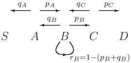
Figure 2: Schematic representation of the five state chain model.

Now, to compute the duration of the game defined in Section 2, we focus on the time spent by a trajectory at any site $i$, namely, we consider the local times $\tau_{i}=|\{t>0:\,x_{t}=i\}|$ for any $i=1,\dots,L-1$, where $|\cdot|$ denotes the cardinality of a set. The fist arrival time to $L$, provided that it exists, can be expressed as the sum of local times on the sites reached by the walk. Hence the conditional expectation $F_{1}$, i.e., the residence time, reads

$$F_{1}=\sum_{i=1}^{L-1}\mathbb{E}_{1}[\tau_{i}|T_{L}<T_{0}]$$ (20)

where $T_{L}<T_{0}$ is the event that the walk reaches $L$ before $0$, i.e., it exits from the left side. As proven in [26], for all $i\in\{1,\ldots,L-1\}$ it holds

$$\begin{split}&\mathbb{E}_{1}[\tau_{i}|T_{L}<T_{0}]=\frac{\mathbb{P}_{1}[T_{i}<T_{0}]}{\mathbb{P}_{1}[T_{L}<T_{0}]}\frac{p_{B}p_{C}}{[1-(r_{B}+p_{B}q_{C}+q_{B}p_{A})]^{2}}\;\;,\end{split}$$ (21)

where

$$\begin{array}[]{ll}p_{A}=\mathbb{P}_{i-1}(T_{i}<T_{0}),&q_{A}=\mathbb{P}_{i-1}(T_{0}<T_{i}),\\ p_{B}=\mathbb{P}_{i}(x_{1}=i+1),&q_{B}=\mathbb{P}_{i}(x_{1}=i-1),\\ p_{C}=\mathbb{P}_{i+1}(T_{L}<T_{i}),&q_{C}=\mathbb{P}_{i+1}(T_{i}<T_{L}).\end{array}$$ (22)

Note that $p_{A}+q_{A}=1$, $p_{B}+q_{B}+r_{B}=1$, and $p_{C}+q_{C}=1$.

Our strategy to compute the residence time is the following: for any $i=1,\dots,L-1$ we shall compute $\mathbb{E}_{1}[\tau_{i}|T_{L}<T_{0}]$ identifying the correct values of $p_{A}$, $q_{A}$, $p_{B}$, $q_{B}$, $p_{C}$, and $q_{C}$ to be used, whose definition depends on the choice of the site $i$. Finally, the sum (20) will provide us with the residence time.

Note that the values of $p_{A}$,$\ldots$,$q_{C}$ have to be searched in the form of $p_{1}$, $p_{2}$, or $p_{3}$ defined in Section 3.1 depending on the value of $i$. The site $i$ can be chosen in five different ways: as a site in the bulk before or beyond the defect, as a site neighboring the defect or as the defect site.

Case $i\leq d-2$. The probability $\mathbb{P}_{1}[T_{i}<T_{0}]$ follows from the classic results on the gambler’s ruin problem. It is $(1-q/p)/(1-(q/p)^{i})$ if $p\neq q$ and $1/i$ if $p=q$. Analogously, $p_{A}$ follows from the same result but starting from $i-1$, so $p_{A}=(1-(q/p)^{i-1})/(1-(q/p)^{i})$ if $p\neq q$ and $(i-1)/i$ if $p=q$. On the other hand, $q_{A}$ can be deduced as $q_{A}=1-p_{A}$, whereas $p_{B}$, $q_{B}$, and $r_{B}$ are respectively $p$, $q$, and $1-p-q$. Finally, $p_{C}$ is the crossing probability for a shorter lane, with $L$ replaced by $L-i$ and initial site $i+1$. From (9) we thus get

$$p_{C}=\frac{p^{\prime}(p-q)q}{p(-p^{\prime}q(-1+(q/p)^{d-i})+p(-(q/p)^{L-i}+(q/p)^{d-i})q^{\prime})}$$

for $p\neq q$, while if $p=q$ it holds $p_{C}=1/(d-i+(L-d-i)q^{\prime}/p^{\prime})$. We also have $q_{C}=1-p_{C}$.

Case $i=d-1$. The probability $\mathbb{P}_{1}[T_{d-1}<T_{0}]$ doesn’t change its form and becomes $(1-q/p)/(1-(q/p)^{d-1})$ if $p\neq q$ and $1/(d-1)$ if $p=q$. In the same way we find $p_{A}=(1-(q/p)^{d-2})/(1-(q/p)^{d-1})$ if $p\neq q$ and $(d-2)/(d-1)$ if $p=q$. The terms $p_{B}$, $q_{B}$, and $r_{B}$ are the same as before, whereas $q_{C}$ has the structure of $p_{2}$ of Section 3.1 but exchanging the role of $p$ and $q$, $p^{\prime}$ and $q^{\prime}$ and the sites before and beyond the defect. Thus, if $p\neq q$

$$q_{C}=\frac{q^{\prime}}{p^{\prime}+q^{\prime}-p^{\prime}[1-(p/q)^{L-d-1}]/[1-(p/q)^{L-d}]}.$$

In the symmetric case, $p=q$, $q_{C}$ reads $q^{\prime}/(1-[p^{\prime}(L-d)/(L-d+1)+1-q^{\prime}-p^{\prime}])$.

Case $i=d$. The probability $\mathbb{P}_{1}[T_{d}<T_{0}]$ is $(1-q/p)/(1-(q/p)^{d})$ if $p\neq q$ and $1/d$ if $p=q$. As in the previous cases, $p_{A}=(1-(q/p)^{d-1})/(1-(q/p)^{d})$ if $p\neq q$ and $(d-1)/(d)$ if $p=q$. Now, $p_{B}=p^{\prime}$, $q_{B}=q^{\prime}$, and $r_{B}=\varepsilon$. Finally, $p_{C}$ is easily find as a gambler’s win probability, $(1-q/p)/(1-(q/p)^{L-d})$ or $1/(L-d)$ for $p\neq q$ and $p=q$ respectively.

Case $i=d+1$. First note that $\mathbb{P}_{1}[T_{d+1}<T_{0}]$ is exactly the product $p_{1}p_{2}$. Moreover, $p_{A}=p_{2}$, $p_{B}=p$, $q_{B}=q$ and $r_{B}=1-p-q$. Finally, $p_{C}$ is again as a gambler’s win probability, $(1-q/p)/(1-(q/p)^{L-d})$ or $1/(L-d)$ for $p\neq q$ and $p=q$ respectively.

Case $i\geq d+2$. First note that $\mathbb{P}_{1}[T_{i}<T_{0}]$ and $q_{A}$ have the form of a crossing probability for a shorter lane, namely,

$$\mathbb{P}_{1}[T_{i}<T_{0}]=\frac{p^{\prime}(p-q)q}{p(-p^{\prime}q(-1+(q/p)^{d})+p(-(q/p)^{i}+(q/p)^{d})q^{\prime})}$$

when $p\neq q$ and it is equal to $1/(d+(L-d-i)q^{\prime}/p^{\prime})$ if $p=q$. To find $q_{A}$ we exchange the role of the probability to jump to the left and to the right, and of sites before and beyond the defect. Thus

$$q_{A}=\frac{q^{\prime}(q-p)p}{q(-q^{\prime}p(-1+(p/q)^{i-d})+q(-(p/q)^{i}+(p/q)^{i-d})p^{\prime})}$$

when $p\neq q$ and $1/(L-d-i+ip^{\prime}/q^{\prime})$ if $p=q$. The probabilities in $B$ and $C$ has the same form of the previous case $i=d+1$.

4 Discussion

In this section we investigate numerically the residence time problem and compare the numerical experiments results to the exact computations carried out in Section 3. We compute numerically the residence time by simulating many particles and averaging the time that each of them takes to exit through the right ending point. The particles exiting through the left ending point are discarded.

We shall discuss our findings providing plots where the solid lines will represent the numerical result and the dots will denote the exact results obtained with the two strategies discussed in Section 3. More precisely, the open and solid dots will denote the representations of the residence time obtained by using, respectively, the local time approach and the generating function method. All the details about the numerical simulations are in the figure captions. The statistical error, since negligible, is not reported in the picture. We fix from now on as the length of the lane $L=100$.

We consider first regular symmetric sites, i.e., $p=q=1/2$, with a defect mimicking a 2D obstacle placed in the right part of the channel, namely, when the particle is on the defect it jumps to the right with probability $p^{\prime}\in(0,1/2]$, to the left with probability $1/2$, and does not move with probability $\varepsilon=1/2-p^{\prime}$. Figure 3 shows the effect that different values of $p^{\prime}$ and $d$ have on residence time. We present the plot of the residence time as a function of $p^{\prime}\in(0,1/2]$ and $d\in\{2,\ldots,98\}$ in the left top panel, where the residence time is calculated with the local time approach. We represent in yellow the value of the residence time measured in absence of defect. The other pictures represent a comparison among the proposed methods of evaluation of the residence time. In the top right picture the values of $p^{\prime}$, $q^{\prime}$, and $\varepsilon$ are fixed respectively to $0.1$, $0.5$, and $0.4$, while $d$ is varied. In the bottom panels the residence time is plotted as a function of $p^{\prime}$ with $d=24$ on the left and $d=74$ on the right. The solid line represents the Monte Carlo results obtained simulating $10^{7}$ particles. The number of particles that eventually cross the lane and contribute to the calculation of the average residence time grows when $p^{\prime}$ and $d$ increase and it varies in the simulations from about $2\times 10^{4}$ to $1\times 10^{5}$. The dashed line represents the value 3333 of the residence time in absence of defect.

Figure 3: Residence time for $L=100$, $p=q=1/2$, and $q^{\prime}=1/2$. the residence time is computed with the local times approach for $p^{\prime}\in[0.005,0.5]$ and $d$ ranging from $2$ to $98$. In the other pictures the solid line represents the Monte Carlo measure obtained simulating $10^{7}$ particles, whereas solid (resp. open) dots represent the generating function (resp. local time method) exact computation. The dashed line denotes the value 3333 of the residence time measured in absence of defect (this value is in yellow in the top left picture). In the top right picture $p^{\prime}=0.1$. In the bottom pictures $d=24$ (left) and $d=74$ (right).

In the case considered in Figure 3 the defect is difficult to be overtaken by the particle since $p^{\prime}\leq 1/2$, thus in the typical trajectories the walker spends a lot of time in the region before the defect. If the defect is close to the left end, it is probable that the particle finally exits the lane through the left side and it does not contribute to the residence time. Thus, in this case the defect selects those particles that quickly overtake it and do not visit again the left part of the lane. This explains why the residence time, for small $d$ and $p^{\prime}$, is smaller than the no defect value. When $d$ is large, namely, the defect is close to the right end of the lane, it becomes more likely that a particle wanders a long time in the left part of the lane before eventually reaching the right side exit. This explains why the residence time for $d>L/2$ is larger than the no defect value. These effects are all negligible when $p^{\prime}$ approaches $1/2$ and so the case of absence of defect is recovered.

In Figure 4 we consider a case which is specular with respect to the one considered in Figure 3: we set $p^{\prime}=1/2$ and vary $q^{\prime}\in(0,0.5]$ with $\varepsilon=1/2-q^{\prime}$. Even in this case different values of $d\in\{2,\ldots,98\}$ are considered. Obviously the results that we find are specular with respect to the line $d=L/2$ with respect to those depicted in the left top panel of Figure 3.

Figure 4: Residence time computed with the local times approach for $L=100$, $p=q=1/2$, $q^{\prime}\in[0.005,0.5]$, $p^{\prime}=1/2$, $\varepsilon=0.5-q^{\prime}$, $d=2,\dots,98$. The residence time value 3333 for the no defect case is represented in yellow.

Still for symmetric regular sites, i.e., $p=q=1/2$, in Figure 5 we consider $p^{\prime}=1-q^{\prime}\in(0,1)$, so that the probability that the particle at the defect does not move is $\varepsilon=0$. The behavior is coherent with that one discussed in the previous cases, with shorter or larger residence time depending on the position of the defect and the ratio $p^{\prime}/q^{\prime}$. If $p^{\prime}=q^{\prime}=1/2$ the no defect case is obviously recovered. Note, and this is less intuitive, that the residence time is the same of the totally symmetric case also if $d=50$, namely, when the defect is at the middle of the lane. As we did before, a comparison among results obtained via different approaches is proposed in Figure 5.

Figure 5: Residence time for $L=100$, $p=q=1/2$, $\varepsilon=0$. On the left the residence time is computed via the local times approach for $p^{\prime}\in[0.01,0.99]$ and $d=2,\dots,98$. The no defect value 3333 of the residence time is represented in yellow. Center panel: residence time vs. $p^{\prime}$ for $d=80$. Right panel: residence time vs. $d$ for $p^{\prime}=0.9$. For the center and right panel lines and symbols are as in Figure 3.

Figure 6: Residence time for $L=100$, $p=0.49$, $q=0.51$, $q^{\prime}=q=0.51$. The top left panel represents the residence time computed with the local times approach for $p^{\prime}\in[0.005,0.49]$ and $d=2,\dots,98$. Lines and symbols are as in Figure 3, but the residence time with no defect is now 2686 and the total number of simulated particles is $10^{8}$. In the top right panel $p^{\prime}=0.1$. In the bottom panels $d=24$ (left) and $d=85$ (right).

The effects shown in Figure 5 for $p^{\prime}\leq 1/2$ and $p^{\prime}\geq 1/2$ are qualitatively the same as those in Figures 3 and 4, respectively. Indeed, since $p^{\prime}\leq 1/2$ implies $q^{\prime}\geq p^{\prime}$, in this case it is more difficult to overtake the defect than to be rejected. Thus, the explanation of the residence time behavior is the same as for the case in Figure 3. Conversely, if $p^{\prime}\geq 1/2$ the behavior is similar to that in Figure 4: for a particle placed on the defect site it is more likely to jump to the right part of the lane and this favors a quick evacuation of the walker if the defect is beyond the middle point of the lane, while it makes difficult for a particle to exit easily from the left side if the walker meets the defect for $d<L/2$.

We now investigate the case in which the regular sites are not symmetric anymore, i.e., $p\neq q$. We first consider the analog of the case in Figure 3, namely, we fix $p$ and $q=1-p$ and vary the defect parameters. At the defect the walker jumps to the left as at regular sites, i.e., $q^{\prime}=q$, but it jumps to the right with a different probability $p^{\prime}\in(0,p]$; as usual $\varepsilon=1-q^{\prime}-p^{\prime}$. In Figure 6 we pick $p=0.49$ and $q=0.51$ and construct the plots analogous to those in Figure 3. The behavior is qualitatively similar to the one in Figure 3: for small values of $p^{\prime}$ and $d$ the residence time is smaller with respect to the no defect case, but at small $p^{\prime}$ it increases when $d$ is increased. The presence of a small adverse drift, i.e., $p<q$, increases the value of $d$ at which the transition between the two effects is observed. As remarked above, the plots in Figure 6 are similar to those in Figure 3, but to perform the Monte Carlo computation many more particles had to be simulated to average on a similar number of particles crossing the lane, with respect to the cases considered before with symmetric regular sites, due to the sensible decreasing of the probability to cross the lane when $p<q$.

Different values of the drift at regular sites modify further the residence time behavior. If $p$ decreases only values of $d$ very close to $L$ produce a larger residence time (see Figure 7, top row, where $p$ is equal to $0.45$ and $0.4$ respectively). If $p$ is larger than $1/2$, it is possible to observe a smaller residence time only if the drift is small, for small values of $d$. In the pictures in Figure 7 bottom row, for $p=0.51$ we can still see particles crossing the lane faster for small $d$ and $p^{\prime}$, while for $p=0.55$ this effect is negligible. In each of these plots it is depicted in yellow the value of residence time for $p^{\prime}=p$ (no defect case). Note that the presence of drift, both if $p<q$ or not, produces in absence of defect a notable reduction of the residence time, see also the right panel in Figure 8.

Figure 7: Residence time computed with the local times approach for $L=100$ and $d=2,\dots,98$. Top left panel: $p=0.45$, $q=0.55$, $p^{\prime}\in[0.005,0.45]$, $q^{\prime}=q$; the value of the residence time in absence of defect is $900$. Top right panel: $p=0.4$, $q=0.6$, $p^{\prime}\in[0.005,0.4]$, $q^{\prime}=q$; the value of the residence time in absence of defect is $475$. Bottom left panel: $p=0.51$, $q=0.49$, $p^{\prime}\in[0.005,0.51]$, $q^{\prime}=q$; the value of the residence time in absence of defect is $2686$. Bottom right panel: $p=0.55$, $q=0.45$, $p^{\prime}\in[0.005,0.55]$, $q^{\prime}=q$; the value of the residence time in absence of defect is $900$. In yellow it is represented the residence time with no defect ($p^{\prime}=p$).

As we did in Figure 4 for the regular symmetric sites case, we could consider the analogous case even in presence of drift. Since the effect is similar we do not report the data in details.

Finally, we summarize our results in Figure 8, where left and right panels report, respectively, the dependence of the residence time on $p^{\prime}$ and $p$ for any value of $d$. In Figure 8 left panel, where $\varepsilon=0$ (hence $p^{\prime}=1-q^{\prime}$), we can notice a behavior similar to the one in Figure 5, but the drift modify the value of $d$ for which the transition between the zones with larger and smaller residence time happens, as observed in Figures 6 and 7. In the picture the small drift case $p=0.49$ and $q=0.51$ is considered.

The right panel, where a defect with $p^{\prime}=0.1$ and $q^{\prime}=0.9$ is considered, points out also that the presence of the drift yields smaller values of the residence time whatever the direction of the drift is. If the drift is directed towards the left end this is due to the fact that only fast particles are selected to exit through the right end of the lane. On the other hand, if the drift is directed towards the right end the effect is simply due to the fact that particles are pushed towards the right end of the lane.

Figure 8: Residence time computed with the local times approach for $L=100$ and $d=2,\dots,98$. Left picture: $p=0.49$, $q=0.51$, $p^{\prime}\in[0.01,0.99]$, $q^{\prime}=1-p^{\prime}$, the value of the residence time in absence of defect is $2686$ (in yellow). Right picture: $p^{\prime}=0.1$, $q^{\prime}=0.9$, $p\in[0.25,0.75]$, $q=1-p$.

As a general remark we notice that the residence time is mainly influenced by the ratios between $q$ and $p$ and between $q^{\prime}$ and $p^{\prime}$. The effect of the probability $\varepsilon$ to remain steady is to increase the residence time by letting grow the local times only on the defect site. This growth is in general not so consistent. Similarly, the probability $r$ acts on regular sites and it produces a growth of a factor $1/(1-r)$ of the local times on each regular site. So, the behaviors with different values of $r$ and $\varepsilon$ can be deduced from the cases presented above, and we will not show further plots for these cases.

References

- [1] E. Cristiani and D. Peri. Applied Mathematical Modelling, 45:285 – 302, 2017.
- [2] M.J. Saxton. Biophysical Journal, 66:394–401, Feb 1994.
- [3] F. Höfling and T. Franosch. Reports on Progress in Physics, 76(4), 2013.
- [4] M.A. Mourão, J.B. Hakim, and S. Schnell. Biophysical Journal, 107:2761–2766, Jun 2017.
- [5] A.J. Ellery, M.J. Simpson, S.W. McCue, and R.E. Baker. The Journal of Chemical Physics, 140(5):054108, 2014.
- [6] K. To, P. Lai, and H.K. Pak. Phys. Rev. Lett., 86:71–74, Jan 2001.
- [7] I. Zuriguel, A. Garcimartín, D. Maza, L.A. Pugnaloni, and J.M. Pastor. Phys. Rev. E, 71:051303, May 2005.
- [8] F. Alonso–Marroquin, S.I. Azeezullah, S.A. Galindo–Torres, and L.M. Olsen-Kettle. Phys. Rev. E, 85:020301, Feb 2012.
- [9] I. Zuriguel, A. Janda, A. Garcimartín, C. Lozano, R. Arévalo, and D. Maza. Phys. Rev. Lett., 107:278001, Dec 2011.
- [10] D. Helbing. Rev. Mod. Phys., 73:1067–1141, Dec 2001.
- [11] D. Helbing, I. Farkas, P. Molnàr, and T. Vicsek. In M. Schreckenberg and S. D. Sharma, editors, Pedestrian and Evacuation Dynamics, pages 21–58, Berlin, 2002. Springer.
- [12] E.N.M. Cirillo and A. Muntean. Physica A: Statistical Mechanics and its Applications, 392(17):3578 – 3588, 2013.
- [13] A. Muntean, E.N.M. Cirillo, O. Krehel, M. Bohm, In “Collective Dynamics from Bacteria to Crowds”, An Excursion Through Modeling, Analysis and Simulation Series: CISM International Centre for Mechanical Sciences, Vol. 553 Muntean, Adrian, Toschi, Federico (Eds.) 2014, VII, 177 p. 29 illus, Springer, 2014.
- [14] E.N.M. Cirillo, A. Muntean, Comptes Rendus Macanique 340, 626–628, 2012.
- [15] A. Ciallella, E.N.M. Cirillo, P.L. Curseu, A. Muntean, Mathematical Models and Methods in Applied Sciences, https://doi.org/10.1142/S0218202518400079.
- [16] G. Albi, M. Bongini, E. Cristiani, and D. Kalise. SIAM Journal on Applied Mathematics, 76(4):1683–1710, 2016.
- [17] D. Helbing, I. Farkas, and T. Vicsek. Nature, 407:487–490, Sep 2000.
- [18] D. Helbing, L. Buzna, A. Johansson, and T. Werner. Transportation Science, 39(1):1–24, 2005.
- [19] R. Escobar and A. De La Rosa. In W. Banzhaf, J. Ziegler, T. Christaller, P. Dittrich, and J.T. Kim, editors, Advances in Artificial Life, Proceedings of the 7th European Conference, ECAL, 2003, Dortmund, germany, September 14–17, 2003, Proceedings. Lecture Notes in Computer Science, vol. 2801., pages 97–106, Berlin, 2003. Springer.
- [20] E.N.M. Cirillo, M. Colangeli, and A. Muntean. Physical Review E 94, 042116 (2016).
- [21] S.A. Janowsky, J.L. Lebowitz, J. Stat. Phys. 77, 35–51 (1994).
- [22] B. Scoppola, C. Lancia, R. Mariani, J. Stat. Phys. 161, 843–858 (2015).
- [23] E.N.M. Cirillo, O. Krehel, A. Muntean, and R. van Santen. Phys. Rev. E, 94:042115, Oct 2016.
- [24] E.N.M. Cirillo, O. Krehel, A. Muntean, R. van Santen, and Aditya S. Physica A: Statistical Mechanics and its Applications, 442:436 – 457, 2016.
- [25] B.W. Fitzgerald, J.T. Padding, and R. van Santen. Phys. Rev. E, 95:013307, Jan 2017.
- [26] A. Ciallella, E.N.M. Cirillo, J. Sohier. Physical Review E, 97:052116, 2018.
- [27] A. Ciallella and E.N.M. Cirillo. Kinetic & Related Models 11, 1475–1501 (2018).
- [28] W. Feller. An Introduction to Probability Theory and its Applications, volume 1. John wiley & Sons, Inc, New York – London – Sidney, 1968.
- [29] F. Stern, Math. Mag. 48, 200–203 (1975).
- [30] T. Lengyel, Applied Mathematics Letters 22, 351–355 (2009).
- [31] E.N.M. Cirillo, M. Colangeli, Phys. Rev. E, 96:052137, 2017.
- [32] D. Andreucci, E.N.M. Cirillo, M. Colangeli, D. Gabrielli. Preprint 2018, arXiv:1807.05167 .