Impact of inter-correlated initial binary parameters on double black hole and neutron star mergers

The distributions of the initial main-sequence binary parameters are one of the key ingredients in obtaining evolutionary predictions for compact binary (BH-BH / BH-NS / NS-NS) merger rates. Until now, such calculations were done under the assumption that initial binary parameter distributions were independent. For the first time, we implement empirically derived inter-correlated distributions of initial binary parameters primary mass ($M_{1}$), mass ratio ($q$), orbital period ($P$), and eccentricity ($e$).

Unexpectedly, the introduction of inter-correlated initial binary parameters leads to only a small decrease in the predicted merger rates by a factor of $\lesssim 2-3$ relative to the previously used non-correlated initial distributions. The formation of compact object mergers in the isolated classical binary evolution favours initial binaries with stars of comparable masses ($q\approx$ 0.5 $-$ 1) at intermediate orbital periods (${\rm log}\,P\,{\rm(days)}$ = 2 $-$ 4). New distributions slightly shift the mass ratios towards lower values with respect to the previously used flat $q$ distribution, which is the dominant effect decreasing the rates. New orbital periods ($\sim$ 1.3 more initial systems within ${\rm log}\,P\,{\rm(days)}$ = 2 $-$ 4), together with new eccentricities (higher), only negligibly increase the number of progenitors of compact binary mergers.

Additionally, we discuss the uncertainty of merger rate predictions associated with possible variations of the massive-star initial mass function (IMF). We argue that evolutionary calculations should be normalized to a star formation rate (SFR) that is obtained from the observed amount of UV light at wavelength 1500$\AA$ (an SFR indicator). In this case, contrary to recent reports, the uncertainty of the IMF does not affect the rates by more than a factor of $\sim 2$. Any change to the IMF slope for massive stars requires a change of SFR in a way that counteracts the impact of IMF variations on compact object merger rates. In contrast, we suggest that the uncertainty in cosmic SFR at low metallicity can be a significant factor at play.

1 Introduction

The Laser Interferometer Gravitational-wave Observatory (LIGO) began its first upgraded observational run (O1) in September 2015; the first ever detection of a gravitational wave signal from a binary black hole (BH-BH) coalescence came shortly afterwards: i.e. GW150914 (Abbott et al. 2016b; c). Since then, four additional BH-BH mergers and, most recently, a double neutron star (NS-NS) merger, were detected and reported to the community: i.e. GW151226 (BH-BH, Abbott et al. 2016a), GW170104 (BH-BH, Abbott et al. 2017a), GW170608 (BH-BH, Abbott et al. 2017b), GW170814 (BH-BH, Abbott et al. 2017c), and GW170817 (NS-NS, Abbott et al. 2017d). The last three events were observed during the second observational run (O2); the Advanced Virgo detector (Acernese et al. 2015) joined the run on August 1, 2017 and contributed to the analysis of GW170814 and GW170817.

The LIGO discovery marks the beginning of the gravitational-wave era. Detections of the coalescence signals from compact binary mergers (CBM) are of utmost astrophysical significance as, among other applications, they will constrain potential formation scenarios, stellar evolution models, and other assumptions associated with theoretical predictions (e.g. Stevenson et al. 2015; O’Shaughnessy et al. 2017; Barrett et al. 2018). Various formation scenarios for CBM have been proposed. Those most widely discussed include the isolated binary evolution channel involving a common envelope (CE) phase (Eldridge & Stanway 2016; Belczynski et al. 2016b; Chruslinska et al. 2018; Mapelli et al. 2017; Giacobbo et al. 2018; Stevenson et al. 2017) or stable mass transfer (van den Heuvel et al. 2017), isolated evolution of field triples (eg. Antonini & Rasio 2016), dynamical evolution in dense stellar environments such as globular clusters (GCs; Rodriguez et al. 2016b; a; Askar et al. 2017; Park et al. 2017), nuclear star clusters (Miller & Lauburg 2009; Antonini & Rasio 2016) or even discs of active galactic nuclei (Stone et al. 2017)), and the formation of compact objects in very close and tidally locked binaries through chemically homogeneous evolution (de Mink & Mandel 2016; Mandel & de Mink 2016; Marchant et al. 2016). We note that while it is still possible to distinguish between different types of mergers (i.e. BH-BH, BH-NS, or NS-NS) in a model-independent way (Mandel et al. 2015; 2017) using their gravitational-wave signatures, we still lack a reliable way to determine the formation channel of an observed merger. This is especially true in case of the LIGO/Virgo NS-NS merger (Belczynski et al. 2017a). In the case of BH-BH mergers there is some hope connected to the measurement of the BH-BH spin-orbit misalignments (Stevenson et al. 2017; Farr et al. 2017; 2018), although this may not work if the BH spins are intrinsically very small (Belczynski et al. 2017b).

Regardless of the formation scenario, the theoretical predictions for the compact binary merger rates are burdened with significant uncertainties due to numerous assumptions and models with poorly constrained parameters, for example the infamous CE phase (Dominik et al. 2012) or the BH/NS natal kicks (Repetto & Nelemans 2015; Belczynski et al. 2016c)). One of the key ingredients in the calculations are the initial conditions for the simulations: the birth properties of stellar clusters in the case of dynamical scenarios and the characteristics of primordial binaries in the case of isolated binary evolution channels.

Recently, de Mink & Belczynski (2015) incorporated the updated primordial binary parameter distributions obtained by Sana et al. (2012) from spectroscopic measurements of massive O-type stars in very young ($\sim$ 2 Myr) open star clusters and associations. The updated distributions included a much stronger bias towards close binary orbits with respect to the previously adopted Öpik’s law, i.e. a flat in logarithm distribution (Öpik 1924; Abt 1983). Intuitively, this change should favour interacting binaries (including those undergoing the CE phase) and possibly cause a notable increase in merger rates. However, de Mink & Belczynski (2015) found only a very small increase of less than a factor of 2. This is because the distributions obtained by Sana et al. (2012) also show a heavy bias towards low eccentricities with respect to the thermal-equilibrium distribution of Heggie (1975); this distribution results in a nearly unchanged distribution of periastron separations, which is the essential separation regulating the onset of mass transfer.

The sample of binaries observed by Sana et al. (2012) suffers from a significant limitation: it is restricted to systems with ${\rm log}\,P\,{\rm(days)}$ $<$ 3.5 (spectroscopically detectable binaries) and dominated by very short-period orbits with P $<$ 20 days (hence the huge fraction of circularized systems). Since the BH-BH mergers can originate from primordial binaries of up to log P $\sim$ 5.5 (de Mink & Belczynski 2015) the binary parameter distributions obtained by Sana et al. (2012) need to be extrapolated to longer periods, which automatically assumes no intrinsic correlations between parameters. However, the joint probability density function cannot be decomposed into independent distribution functions of the individual parameters, i.e. $f(M_{1},q,P,e)\neq f(M_{1})f(q)f(P)f(e)$. Observational studies have hinted at probable correlations (Abt et al. 1990; Duchêne & Kraus 2013), but hitherto the selection biases have been too large to accurately quantify the intrinsic interrelations. Recently, Moe & Di Stefano (2017; hereafter MD17) analysed more than 20 surveys of massive binary stars, corrected for their respective selection effects, combined the data in a homogeneous manner, and fit analytic functions to the corrected distributions. These authors confirm that many of the physical binary star parameters are indeed correlated at a statistically significant level.

de Mink & Belczynski (2015) concluded that the most significant variations of merger rates associated with the initial parameters are due to uncertainties of the initial mass function (IMF) power-law slope for massive stars (merger rates going up and down by a factor of six in the case of BH-BH). Cosmological calculations of the BH-BH merger rates (e.g. Dominik et al. 2013; 2015; Belczynski et al. 2016b; Kruckow et al. 2018; Mapelli et al. 2017) are performed based on the assumption of a universal IMF across the cosmic time. Often assumed is a so-called “canonical” IMF, which is a multi-part power-law distribution $dN/dM=\xi(M)\propto M^{-\alpha_{i}}$, where $\alpha_{1}=1.3$ for $M/M_{\odot}\in[0.08,0.5]$ and $\alpha_{2}=\alpha_{3}=2.3$ for $M/M_{\odot}\in[0.5,1.0]$ and $[1.0,150.0]$, respectively (Kroupa 2001).

Although clear evidence for strong IMF variations with environmental conditions is still lacking, there are a growing number of results hinting at departures from the IMF universality (see reviews by Bastian et al. 2010; Kroupa et al. 2013). Notably, a recent spectroscopic survey of massive stars in the 30 Doradus star-forming region in the Large Magellanic Cloud has led to a discovery of an excess of stars with masses above $30{\leavevmode\nobreak\ M}_{\odot}$ with respect to the canonical IMF (Schneider et al. 2018); the best-fitted single power-law exponent for $M>1{\leavevmode\nobreak\ M}_{\odot}$ is $\alpha_{3}=1.90_{-0.26}^{+0.37}$ (although see a technical comment on the data analysis from Farr & Mandel 2018; suggesting somewhat larger values for $\alpha_{3}$).

The unknowns associated with the massive-star IMF are often considered to be one of the significant contributors to uncertainty of compact binary merger rates calculated based on population synthesis. In this work, we argue that by normalizing the simulated stellar population to the total amount of far-UV light that it emits, rather than to its total mass, one can significantly reduce the uncertainty associated with possible variations of the IMF slope in different environments; see Sect. 6.2. As an example of such a variation and its impact on merger rate calculations, we study in detail the case of a possible correlation between the massive-star IMF slope and metallicity Z.

With the exception of above-mentioned results of Schneider et al. (2018), numerous observations of OB associations and clusters in the Local Group did not reveal any significant deviations from the canonical IMF slope for massive stars $\alpha_{3}\approx 2.3$ (Massey 2003). These included surveys of the Milky Way (Z $\approx{\leavevmode\nobreak\ Z}_{\odot}$ = 0.02; Daflon & Cunha 2004) , the Small Magellanic Cloud (Z $\approx$ 0.004; Korn et al. 2000) and the Large Magellanic Cloud (Z $\approx$ 0.008; Korn et al. 2000), indicating that for Z $\geq$ 0.004 ([Fe/H] $\gtrsim-0.7$) the high-mass end of IMF does not significantly depend on metallicity. Moe & Di Stefano (2013) showed that the same is true for the parameters of close binaries with massive stars. Even at solar metallicity, the discs of massive protostars are already highly prone to gravitational instability and fragmentation, explaining why the close binary fraction of massive stars is so large (Kratter & Matzner 2006; Kratter et al. 2008; 2010; Moe & Di Stefano 2017). Further reducing the metallicity can therefore only marginally increase the close binary fraction of massive stars (Tanaka & Omukai 2014; Moe et al. 2018). However, as we show, the vast majority of BH-BH mergers evolving from the CE channel are expected to originate from Z $<$ 0.004 environments, for which there is no direct observational evidence for the persistence of the canonical IMF.

From a theoretical point of view, both the Jeans-mass formalism (Jeans 1902; Larson 1998; Bate & Bonnell 2005; Bonnell et al. 2006) and the model of stellar formation as a self-regulated balance between the rate of accretion from the proto-stellar envelope and the radiative feedback from the forming star (Adams & Fatuzzo 1996) predict that at a certain sufficiently low metallicity the IMF becomes top heavy . In the first case, the prediction comes from the fact that the Jeans mass has to be larger at lower Z owing to less effective cooling of the proto-stellar cloud ($M_{J}\propto\rho^{-1/2}T^{3/2}$). The radiative feedback, on the other hand, is also metallicity dependent since photons couple less effectively to gas of lower metallicity. Hydrodynamical simulations of the formation of Population III stars ($\rm Z/Z_{\odot}$ $<$ 10^-6) demonstrate that the first generation of stars were almost exclusively massive OB-type main-sequence (MS) stars (Bromm et al. 1999; Yoshida et al. 2006; Clark et al. 2011). However, by redshift $z$ $\approx$ 10, the mean metallicity of actively forming stars was $\rm Z/Z_{\odot}$ $\approx$ 10^-3 (Tornatore et al. 2007; Madau & Dickinson 2014). For such Population II stars with intermediate metallicities, the IMF is expected to be only moderately top heavy compared to the canonical IMF (Fang & Cen 2004; Daigne et al. 2006; Greif et al. 2008).

From the observational side, there is indirect evidence for top-heavy IMF variations at cosmological times. The relative paucity of metal-poor G-dwarf stars in the Milky Way (the so-called G-dwarf problem; Pagel 1989) can be explained by applying an IMF, which is increasingly deficient in low-mass stars the earlier the star formation took place (Larson 1998). By modelling the abundances of Lyman-break and submillimetre galaxies in the $\Lambda$CDM cosmology, Baugh et al. (2005) found that the observations can be reproduced only if some episodes of star formation with a top-heavy IMF were also present in addition to the canonical IMF. Nagashima et al. (2005) used the same model with two modes of star formation to explain the elemental abundances in the intracluster medium of galaxy clusters. Wilkins et al. (2008) pointed out that the local stellar mass density is significantly lower than the value obtained from integrating the cosmic star formation history with a Salpeter IMF (single slope, $\alpha=2.35$; Salpeter 1955). At low redshifts (z $<$ 0.5) they manage to match the observations using a slightly top-heavy ($\alpha_{3}=2.15$) IMF. For higher redshifts, however, Wilkins et al. (2008) argued that no universal IMF can reproduce the measured stellar mass densities.

The only quantitative calibration of the relation between the high-mass IMF and metallicity obtained thus far has been made possible thanks to the observations of some GCs in the Milky Way. Djorgovski et al. (1993) noticed that the higher metallicity GCs tend to have a bottom-light present day mass function (i.e. a deficit of low-mass stars). De Marchi et al. (2007) later found that these GCs are also the least concentrated sources in their observed sample. Such a trend contradicts basic cluster evolution theory – GCs are expected to be losing low-mass stars from their outer regions owing to their collapse into dense, highly concentrated clusters. An explanation was put forth by Marks et al. (2008), who proposed that low-mass stars could be unbound from mass-segregated GCs during expulsion of their residual gas. This introduces a dependence on metallicity, since the process of gas expulsion is expected to be enhanced in metal-rich environments (Marks & Kroupa 2010). Finally, Marks et al. (2012) concluded that in order to provide enough radiative feedback to expel the residual gas and match the characteristics of the observed GCs, their IMF had to be top heavy with the value of $\alpha_{3}$ decreasing with cluster metallicity.

It should be noted, however, that the model of residual gas expulsion applied by Marks et al. (2012) relies on simplified assumptions concerning the radiative feedback. First, the amount of energy deposited from stars into the ISM is fitted to stellar models of only three different masses (35, 60, and 85 ${\leavevmode\nobreak\ M}_{\odot}$; Baumgardt et al. 2008), and second there is no metallicity dependence. Additionally, Marks et al. (2012) assumed that the energy needed for residual gas removal is provided by the stellar winds and radiation only (e.g. no feedback from supernova taken into account) and that all the energy radiated by the stars is deposited into the ISM. Thus, the exact relation between the high-mass IMF slope and metallicity remains highly uncertain.
The purpose of this study is twofold. First, we aim to incorporate the interrelated initial binary parameter distributions and multiplicity statistics obtained by MD17 to determine their effects on the predicted rates and properties of CBM. Second, we investigate the importance of possible IMF variations for the merger rate calculations using the Marks et al. (2012) calibration of the IMF dependency on metallicity as an example of such a variation. To achieve this, we perform comparative population synthesis where we use the works of de Mink & Belczynski (2015) and Belczynski et al. (2016b) as references (hereafter dMB15 and B16, respectively). In Sect. 2 we describe the new initial conditions and compare these with the previously used distributions. In Sect. 3 we describe our computational method. In Sect. 4 we compare the distributions of the initial parameters of double compact merger progenitors in our simulations. In Sect. 5 we present the impact of the incorporated changes on the cosmological merger rates. In Sect. 6 we discuss the metallicity distribution of BH-BH mergers in our simulations and the significance of the top-heavy IMF in low-Z environments for the LIGO predictions. We conclude in Sect. 7.

2 Initial distributions

2.1 Inter-correlated initial binary parameters

In the present study, we account for intrinsic correlations between the initial binary star physical parameters. We used the distribution functions presented in section 9 of MD17. The correlations in the MS binary initial conditions are thoroughly discussed in that paper, but we summarize in this section the main results pertinent to the formation of compact objects mergers. dMB15 found that the majority of compact object mergers derive from MS binaries with initial orbital periods ${\rm log}\,P\,{\rm(days)}$ = 2$-$4. Although for our simulations we generated companions across all orbital periods according to the distribution functions provided in MD17, in this section we focus the discussion on the companion star properties across intermediate periods ${\rm log}\,P\,{\rm(days)}$ = 2$-$4.

Binaries versus triples: dMB15 and B16 assumed all companions to massive stars (M$>$10$\,M_{\odot}$) were in binaries. In contrast, MD17 have modelled a companion star fraction and period distribution that includes true binaries as well as inner binaries and outer tertiaries in hierarchical triples. With increasing orbital period, the likelihood that a companion is an outer tertiary must increase. In fact, essentially all wide companions (${\rm log}\,P>5$) to massive stars are the outer tertiaries in hierarchical triples/quadruples (Sana et al. 2014; MD17). We model the probability that a companion is in the inner binary ${\cal P}_{\rm bin}(M_{1},P)$ in a manner that reproduces the multiplicity statistics derived in MD17. Specifically, for $M_{1}$ = $8{\leavevmode\nobreak\ M}_{\odot}$, we find the probability decreases from ${\cal P}_{\rm bin}$ = 0.96 for ${\rm log}\,P$ = 2 to ${\cal P}_{\rm bin}$ = 0.60 for ${\rm log}\,P$ = 4. For $M_{1}$ = $30{\leavevmode\nobreak\ M}_{\odot}$, the triple/quadruple star fraction is larger, and so we adopt ${\cal P}_{\rm bin}$ = 0.93 for ${\rm log}\,P$ = 2 and ${\cal P}_{\rm bin}$ = 0.23 for ${\rm log}\,P$ = 4. We illustrate ${\cal P}_{\rm bin}(M_{1},P)$ in Fig. 1.

Companion star fraction: dMB15 and B16 implemented a binary star fraction such that F${}_{\rm logP=2-4;bin}\approx$ 28% of massive primaries had binary star companions with periods ${\rm log}\,P\,{\rm(days)}$ = 2$-$4 and mass ratios $q$ = 0.1$-$1.0. The companion star fraction increases dramatically with primary mass (Abt et al. 1990; Raghavan et al. 2010; Sana et al. 2012; Chini et al. 2012; Duchêne & Kraus 2013; Moe & Di Stefano 2013; 2017). According to MD17, the intermediate-period companion star fraction increases from F_{logP=2-4;comp} = 0.46 for $M_{1}$ = $8{\leavevmode\nobreak\ M}_{\odot}$ to F_{logP=2-4;comp} = 0.66 for $M_{1}$ = $30{\leavevmode\nobreak\ M}_{\odot}$. Approximately two-thirds of O-type primaries have a companion with ${\rm log}\,P\,{\rm(days)}$ = 2$-$4 and $q>0.1$. A significant fraction of these systems, especially those with longer periods ${\rm log}\,P\,{\rm(days)}$ = 3.5$-$4.0, are actually outer tertiaries in triples (see above and Fig. 1).

Period distribution: dMB15 and B16 adopted a power-law binary period distribution $f_{\rm logP;bin}$ $\propto$ (log $P$)^-0.55 motivated by spectroscopic observations of massive binaries (Sana et al. 2012). These works normalize this period distribution such that integration F_logP=2-4;bin = $\int_{2}^{4}f_{\rm logP;bin}{\rm d(logP)}$ = 0.28 reproduces the binary fraction across ${\rm log}\,P\,{\rm(days)}$ = 2$-$4. In the current study, we adopt a companion star period distribution $f_{\rm logP;comp}(M_{1},P)$ based on the analytic fits in MD17 that are shown in the lower panel of their Fig. 37. We then derive the inner binary period distribution $f_{\rm logP;bin}$ = $f_{\rm logP;comp}\times{\cal P}_{\rm bin}$. In Fig. 1, we show $f_{\rm logP;bin}$ from dMB15 and B16, $f_{\rm logP;comp}$ for $M_{1}$ = $8{\leavevmode\nobreak\ M}_{\odot}$ and $30{\leavevmode\nobreak\ M}_{\odot}$ taken directly from MD17, and $f_{\rm logP;bin}$ for $M_{1}$ = $8{\leavevmode\nobreak\ M}_{\odot}$ and $30{\leavevmode\nobreak\ M}_{\odot}$ implemented in the current study. While companions in general are weighted towards longer periods, the inner binary period distribution is skewed towards shorter periods as implemented in dMB15 and B16 and found in Sana et al. (2012).

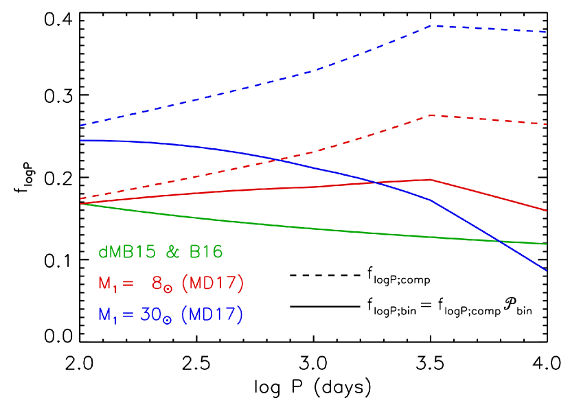
Figure 1: Frequency f_logP of companions with $q$ $>$ 0.1 per decade of orbital period across ${\rm log}\,P\,{\rm(days)}$ = 2$-$4. We compare the distribution f_logP;comp of all companions (binaries and tertiaries; dashed) to the distribution f_logP;bin = f${}_{\rm logP;bin}\times{\cal P}_{\rm bin}$ of only the inner binaries (solid), where ${\cal P}_{\rm bin}$ is the probability that the companion is a member of the inner binary. The overall binary fraction and binary period distribution across ${\rm log}\,P\,{\rm(days)}$ = 2$-$4 are similar between those adopted by dMB15 and B16 (green) and the values for $M_{1}$ = $8{\leavevmode\nobreak\ M}_{\odot}$ (red) and $M_{1}$ = $30{\leavevmode\nobreak\ M}_{\odot}$ (blue) primaries based on the multiplicity statistics presented in MD17.

Eccentricity distribution: dMB15 and B16 incorporated a power-law eccentricity distribution $p_{e}$ $\propto$ $e^{\eta}$ with exponent $\eta$ = $-$0.4 across the domain $e$ = 0.0$-$0.9 , as motivated by Sana et al. (2012). However, the Sana et al. (2012) sample of spectroscopic binaries are dominated by systems with P $<$ 20 days, therefore the power-law slope $\eta$ = $-$0.4 is only appropriate for such short-period systems. MD17 have found that eccentricities become weighted towards higher values with increasing orbital period, which they model with two parameters. First, MD17 have defined the domain of the eccentricity distribution across the interval $e$ = 0.0–$e_{\rm max}$, where $e_{\rm max}(P)$ is the maximum eccentricity possible without substantially filling the Roche lobes of the binary (Eqn. 3 in MD17). For P = 5 days, the binaries must have $e$ $<$ $e_{\rm max}$ $\approx$ 0.5 to be initially non-Roche-lobe filling. Meanwhile, binaries with ${\rm log}\,P\,{\rm(days)}$ = 2$-$4 can extend up to $e_{\rm max}$ $\approx$ 0.95. Second, MD17 have found the power-law slope $\eta$ also increases with increasing period. For massive binaries, they fit $\eta$ $\approx$ 0.8 for ${\rm log}\,P\,{\rm(days)}$ = 2$-$4. We adopt the power-law slopes $\eta(M_{1},P)$ presented in MD17 across the domain $e$ = 0$-$0.8$e_{\rm max}$. At high eccentricities $e$ = (0.8$-$1.0)$e_{\rm max}$, we assume the probability distribution function turns over according to a decreasing linear function such that $p_{e}$($e$ = $e_{\rm max}$) = 0. In Fig. 2, we compare the cumulative distribution function of the eccentricity distribution adopted in dMB15 and B16 to the updated distributions at ${\rm log}\,P\,{\rm(days)}$ = 2 and 4. As expected, the eccentricity distribution based on the Sana et al. (2012) sample is skewed towards lower values.

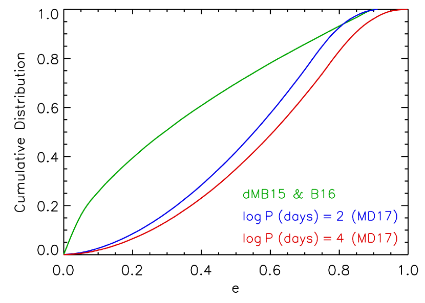
Figure 2: Cumulative distribution function of eccentricities. dMB15 and B16 adopted an eccentricity distribution $p_{e}$ $\propto$ $e^{-0.4}$ (green) based on a sample of massive spectroscopic binaries (Sana et al. 2012) that are dominated by short-period systems P $<$ 20 days and therefore weighted towards lower eccentricities $<$ $e$ $>$ = 0.3. MD17 (and references therein) found that massive binaries with intermediate (blue) and long (red) orbital periods are weighted towards higher eccentricities $<$ $e$ $>$ = 0.6 and are sufficiently modelled by a power-law distribution $p_{e}$ $\propto$ $e^{0.8}$ with a turnover above $e$ $>$ 0.8.

Mass ratio distribution: dMB15 and B16 adopted a uniform mass-ratio distribution $f_{q}$ = $q^{0}$. Again, this was based on a sample of massive spectroscopic binaries (Sana et al. 2012) that is dominated by short-period systems $P$ $<$ 20 days. Based on a series of observational evidence (long baseline interferometry, companions to Cepheids, eclipsing binaries, adaptive optics, Hubble imaging, etc.), MD17 have demonstrated that slightly wider massive binaries are weighted considerably towards smaller mass ratios. Across intermediate periods ${\rm log}\,P\,{\rm(days)}$ = 2$-$4, MD17 have found the mass-ratio distribution is accurately described by a two-component power-law $p_{q}$ $\propto$ $q^{\gamma}$ with slopes $\gamma_{\rm smallq}$ across small mass ratios $q$ = 0.1$-$0.3 and $\gamma_{\rm largeq}$ across large mass ratios $q$ = 0.3$-$1.0. For massive binaries and ${\rm log}\,P\,{\rm(days)}$ = 2, MD17 have fit $\gamma_{\rm smallq}$ = 0.0 and $\gamma_{\rm largeq}$ = $-$1.4, while for ${\rm log}\,P\,{\rm(days)}$ = 4, they have measured $\gamma_{\rm smallq}$ = $-$0.7 and $\gamma_{\rm largeq}$ = $-$2.0 (see their Fig. 35). In Fig. 3, we compare the cumulative mass-ratio distributions used by dMB15 and B16 to the updated distributions measured at ${\rm log}\,P\,{\rm(days)}$ = 2$-$4.

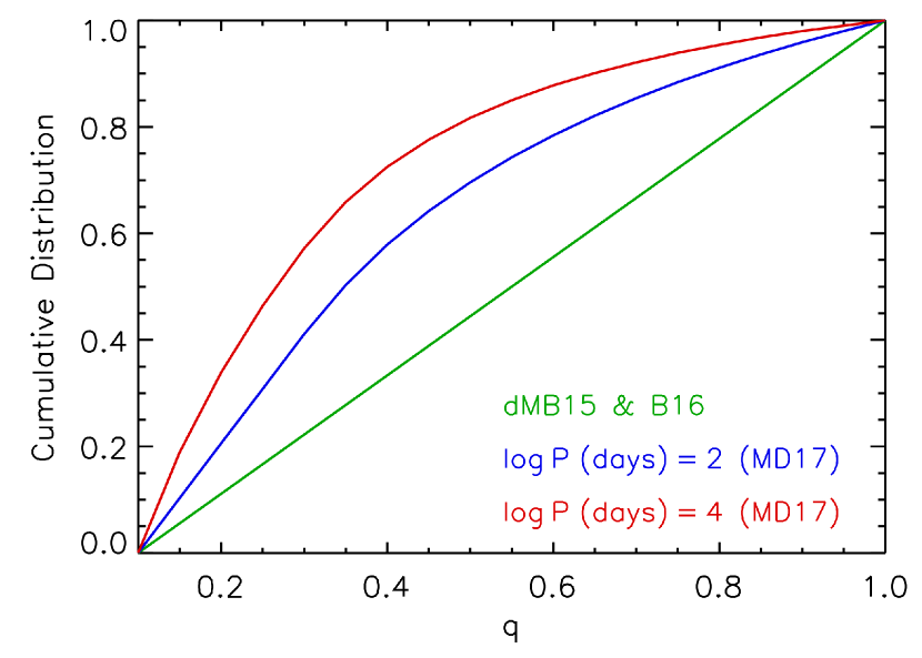
Figure 3: Cumulative distribution function of mass ratios. dMB15 and B16 adopted a uniform mass-ratio distribution $p_{q}$ $\propto$ $q^{0}$ (green) based on a sample of massive spectroscopic binaries (Sana et al. 2012) that are dominated by short-period systems P $<$ 20 days. MD17 (and references therein) found that massive binaries with intermediate periods (blue and red) are weighted significantly towards smaller mass ratios.

Very massive binaries: At present, there are no reliable observational measurements of the properties of very massive binaries with intermediate periods ${\rm log}\,P\,{\rm(days)}$ = 2$-$4 and primary masses $M_{1}$ $>$ $40{\leavevmode\nobreak\ M}_{\odot}$. At these intermediate separations, the mass-ratio and eccentricity distributions do not significantly change across primary masses $8{\leavevmode\nobreak\ M}_{\odot}$ $<$ $M_{1}$ $<$ $40{\leavevmode\nobreak\ M}_{\odot}$. In addition, the inner binary fraction and inner binary period distribution across ${\rm log}\,P\,{\rm(days)}$ = 2$-$4 varies only slightly across the primary mass interval $8{\leavevmode\nobreak\ M}_{\odot}$ $<$ $M_{1}$ $<$ $40{\leavevmode\nobreak\ M}_{\odot}$ (see Fig. 1). We therefore assume that systems with $M_{1}$ $>$ $40{\leavevmode\nobreak\ M}_{\odot}$ have the same period, eccentricity, mass-ratio distributions, and binary fractions as those systems with $M_{1}$ = $40{\leavevmode\nobreak\ M}_{\odot}$.

Triple-star evolution: We model the evolution of all inner binaries with StarTrack. For triples, we ignore the outer tertiaries except for the following case. If the inner binary initially has P $<$ 5 days and q $<$ 0.4, it most likely will undergo unstable Case A Roche lobe overflow (RLOF), merge on the MS, and effectively evolve as a single star. If the tertiary has log $P_{\rm outer}$ (days) $\lesssim$ 4, then such a triple may lead to the formation of compact object merger. We model these triples with inner binaries $P_{\rm bin}$ $<$ 5 days and $q_{\rm bin}$ $<$ 0.4 as simple binaries, where the original inner binary merges to become the effective primary with combined mass $M_{1}$ + $M_{2}$ and the tertiary becomes the effective binary companion with mass $M_{3}$. For simplicity, we assume no rejuvenation of the merger product, i.e. evolve it as a star with the same age as its companion with mass $M_{3}$. About 10% of massive inner binaries with $P$ $<$ 5 days have outer tertiaries in tight, hierarchical configurations log $P_{\rm outer}$ (days) $<$ 4 (MD17). This triple-star channel certainly does not dominate, but can contribute an additional $\approx$5–10% to the overall compact merger rate.

2.2 IMF and its dependence on metallicity

We adopt the same IMF that was used by B16, as guided by the recent observations (Bastian et al. 2010),

$$dN/dM=\xi(M)\propto\begin{cases}M^{-1.3},&\text{for }M/M_{\odot}\in[0.08,0.5]\\ M^{-2.2},&\text{for }M/M_{\odot}\in[0.5,1.0]\\ M^{-\alpha_{3}},&\text{for }M/M_{\odot}\in[1.0,150.0]\end{cases},$$ (1)

where for our standard model $\alpha_{3}$ = $2.3;$ we note that dMB15 adopt $\alpha_{3}$ = $2.7$ but also investigate $\alpha_{3}$ = $2.2$ and $3.2$).

Additionally we calculate a model in which the IMF slope for massive stars depends on metallicity, as described below. In the following, we assume a conversion between [Fe/H] and Z given by Bertelli et al. (1994), appropriate for stars with solar-like fraction of iron among all the metal components.

Based on the observations of stellar clusters in the Milky Way and N-body simulations (Sect. 1) Marks et al. (2012) calibrated that $\alpha_{3;{\rm Marks}}=2.63+0.66$[Fe/H] for [Fe/H] $<$ $-0.5$, which corresponds to Z $\lesssim$ 0.0063. We note that the above relation comes from a rather uncertain fit (see Fig. 4 of Marks et al. 2012) and is based on a model with several caveats (see discussion at the end of Sect. 1). Because the observations of OB associations and clusters in the Local Group do not support any significant deviations from $\alpha$ = 2.3 for metallicities Z $\geq$ 0.004 (Massey 2003), we modify the relation for $\alpha_{3}$ proposed by Marks et al. (2012) such that the IMF dependence towards lower metallicity does not occur until $\rm Z<0.004$, and $\alpha_{3}$ = 2.3 for $\rm Z\geq 0.004$. Marks et al. (2012) observational data extends down to about Z = 0.0001 ([Fe/H] $\approx$ $-$2.3, see their Fig. 4), and we decided to limit the further decrease of $\alpha_{3}$ for lower metallicities. Explicitly we adopt the following formula:

$$\alpha_{3}({\rm Z})=\begin{cases}2.3,&\text{for }Z\geq 0.004\\ 2.3+0.76\,[{\rm log\;Z}+2.4],&\text{for }0.0001<Z<0.004\\ 1.1,&\text{for }Z<0.0001\end{cases}.$$ (2)

For some example values of Z, this formula yields $\alpha_{3}$(Z = $0.1{\leavevmode\nobreak\ Z}_{\odot}$) = 2.07 and $\alpha_{3}$(Z = $0.01{\leavevmode\nobreak\ Z}_{\odot}$) = 1.31.

We note that we treat the IMF d$N/$d$M$ (all stars) and primary mass function d$N/$d$M_{1}$ (single stars and primaries in binaries) interchangeably. Across large masses $M$ $>$ $1{\leavevmode\nobreak\ M}_{\odot}$, both the IMF and primary mass function have the same slope $\alpha_{3}$ = 2.3 (Kroupa et al. 2013). The IMF and primary mass function only differ slightly across small masses $M$ $<$ $1{\leavevmode\nobreak\ M}_{\odot}$. Since $\alpha_{3}$ (and its dependence on metallicity) is the most important parameter for determining merger rates, the assumption that d$N/$d$M$ equals d$N/$d$M_{1}$ is justified.

3 Computational method

3.1 Physical assumptions – the StarTrack code

We utilized the StarTrack population synthesis code (Belczynski et al. 2002; 2008; Dominik et al. 2012). StarTrack is developed based on analytical formulae for the evolution of a non-rotating star obtained by Hurley et al. (2000) from the fits to the grid of evolutionary tracks calculated by Pols et al. (1998). The original Hurley et al. (2000) models were updated with the prescriptions for the wind mass loss from O-B type stars (Vink et al. 2001), Wolf-Rayet stars (Hamann & Koesterke 1998; Vink & de Koter 2005), and enhanced mass loss rates for luminous blue variables (Belczynski et al. 2010a). For core-collapse supernovae we adopt the convection driven, neutrino enhanced “rapid” supernova engine from Fryer et al. (2012), which reproduces the observed mass gap between NSs and BHs (Belczynski et al. 2012). The key parameter of this model, dependent on the mass of the CO core at the time of explosion, is the fraction of material ultimately falling back onto the proto compact object ($f_{b}$) and contributing to the final remnant mass. The supernova kick velocity is drawn from a Maxwellian distribution with $\sigma_{1D}$ = 265$\,\rm{km}\,\rm{s}^{-1}$(Hobbs et al. 2005) and lowered proportionally to the amount of fallback, i.e. $V_{NK}$ = $V_{NK;Hobbs}(1-f_{b})$. This effectively means that the most massive BHs in our simulations (up to $\sim$ 15${\leavevmode\nobreak\ M}_{\odot}$ for ${\leavevmode\nobreak\ Z}_{\odot}$ and $\sim$ 40${\leavevmode\nobreak\ M}_{\odot}$ for $0.1{\leavevmode\nobreak\ Z}_{\odot}$) are also typically those that receive a relatively small or zero natal kick (direct collapse).

We calculated the CE evolution in one step by applying the energy balance prescription of Webbink (1984). We adopt $\alpha_{\rm CE}$ = 1 for the efficiency of energy transfer. The envelope binding parameter $\lambda$ is taken from the fits of Xu & Li (2010) and depends on the radius and the evolutionary state of the donor. There are large uncertainties concerning the stability of mass transfer initiated by a Hertzsprung gap (HG) donor star. Pavlovskii et al. (2017) recently reported that for a large range of donor radii and masses such mass transfer may actually be stable, rather than leading to a CE phase. While revised criteria for a range of different metallicities and other parameters are still under preparation (Ivanova, private communication), we opted to not follow the evolution of systems with HG donors in which our standard criteria for the mass transfer stability (Eq. 49 of Belczynski et al. 2008) indicate a dynamically unstable event.

Up until this point our physical assumptions are the same as in submodel B of dMB15 and standard model M1 of B16. The only recent update is the addition of mass loss due to pair-instability pulsations (model M10; Belczynski et al. 2016a). Such pulsations can affect stars with massive helium cores $M_{\rm He}$ between $\sim$ 40$-$45${\leavevmode\nobreak\ M}_{\odot}$ and $\sim$ 60$-$65${\leavevmode\nobreak\ M}_{\odot}$ and deplete them of a significant amount of mass ($M_{\rm ejecta}\sim$ 5$-$20${\leavevmode\nobreak\ M}_{\odot}$; Heger & Woosley 2002). We modelled this by assuming that stars with $M_{\rm He}$ = 45$-$65${\leavevmode\nobreak\ M}_{\odot}$ are subject to pair-instability pulsations and lose all their mass above 45${\leavevmode\nobreak\ M}_{\odot}$. We note that the inclusion of pair-instability mass loss does not affect our predictions for detections of double compact mergers with the LIGO O2 observational run sensitivity (Belczynski et al. 2016a), and is consistent with existing data (Fishbach & Holz 2017).

3.2 Cosmological calculations of the merger rates

We placed our simulated systems into a cosmological background by populating the Universe up to $z$ = 15. We modelled binaries across 32 different metallicities covering the range from 0.005${\leavevmode\nobreak\ Z}_{\odot}$ to 1.5${\leavevmode\nobreak\ Z}_{\odot}$. In our standard model (I1) the IMF does not depend on metallicity, and so for each Z we use the same sample of $2\times 10^{6}$ systems (single stars, binaries, triples) generated according to the multiplicity statistics described in Sect. 2 and a primary mass function $\xi(M_{1})$ $\propto$ $M_{1}^{-\alpha_{3}}$ with $\alpha_{3}$ = 2.3 across $5{\leavevmode\nobreak\ M}_{\odot}$ $<$ $M_{1}$ $<$ $150{\leavevmode\nobreak\ M}_{\odot}$. We only evolve binaries ($\sim$ 72% of systems with $M_{1}$ $>$ 5${\leavevmode\nobreak\ M}_{\odot}$) and hierarchical triples ($\sim$ 3.6%), in which the inner binary is likely to merge during an early case A mass transfer (Sect. 3). For submodel I2 we assume the metallicity-dependent primary mass function according to Eqn. 2, and for each Z we generate a corresponding sample of $10^{6}$ initial systems.

We calculate the merger rate density as a function of redshift by integrating through the cosmic star formation rate (SFR) history as described in see Sect. 4 of Dominik et al. (2015) and Sect. 2.2 of Belczynski et al. (2016c). For each redshift bin $\Delta z$ = 0.1 up to $z$ = 15 we use the cosmic SFR

$${\rm SFR}(z)=0.015\frac{(1+z)^{2.7}}{1+[(1+z)/2.9]^{5.6}}\leavevmode\nobreak\ {\rm M}_{\odot}{\rm Mpc}^{-3}{\rm yr}^{-1}$$ (3)

from Madau & Dickinson (2014) as implemented in B16. The contribution from each of the metallicities in our simulations at a given redshift of star formation $z_{\rm SF}$ is then calculated as a fraction of SFR($z_{\rm SF}$) according to the mean metallicity evolution model from Madau & Dickinson (2014), increased by 0.5 dex to better fit observational data (Vangioni et al. 2015), i.e.

$$\log(Z_{\rm mean}(z))=0.5+\log\left({y\,(1-R)\over\rho_{\rm b}}\int_{z}^{20}{97.8\times 10^{10}\,{\rm SFR}(z^{\prime})\over H_{0}\,E(z^{\prime})\,(1+z^{\prime})}dz^{\prime}\right).$$ (4)

We adopt a return fraction $R=0.27$ (fraction of stellar mass returned into the interstellar medium), a net metal yield of $y=0.019$ (mass of metals ejected into the medium by stars per unit mass locked in stars), a baryon density $\rho_{\rm b}=2.77\times 10^{11}\,\Omega_{\rm b}\,h_{0}^{2}\,{\leavevmode\nobreak\ M}_{\odot}\,{\rm Mpc}^{-3}$ with $\Omega_{\rm b}=0.045$ and $h_{0}=0.7$, a SFR from Eqn. 3, and $E(z)=\sqrt{\Omega_{\rm M}(1+z)^{3}+\Omega_{\rm k}(1+z)^{2}+\Omega_{\Lambda})}$ in a flat cosmology with $\Omega_{\Lambda}=0.7$, $\Omega_{\rm M}=0.3$, $\Omega_{\rm k}=0$, and $H_{0}=70.0\,{\rm km}\,{\rm s}^{-1}\,{\rm Mpc}^{-1}$. We assume a log–normal distribution of metallicity with $\sigma=0.5$ dex around the mean value at each redshift (Dvorkin et al. 2015).

Madau & Dickinson (2014) obtained their cosmic SFR based on the far-UV (FUV; 1500 $\AA$) and IR (8$-$1000 $\mu{\rm m}$) luminosity functions. Both are regarded as good tracers of star formation as they are dominated by the contribution from short-lived massive stars: FUV directly and IR through re-radiation of dust-absorbed UV. Specifically, Madau & Dickinson (2014) converted strength of the 1500 $\AA$ line in the UV spectrum $L_{\nu}({\rm FUV})$ into a cosmic SFR by applying an adequate conversion factor ${\cal K}_{\rm FUV}$, such that ${\rm SFR}={\cal K}_{\rm FUV}\times L_{\nu}({\rm FUV})$ (their Eqn. 10). To calculate ${\cal K}_{\rm FUV}$ they assume a Salpeter IMF with slope $\alpha$ = 2.35 across masses $M$ = 0.1$-$100${\leavevmode\nobreak\ M}_{\odot}$ (Salpeter 1955). It is therefore inconsistent to implement the above Eqn. 3 in combination with a more realistic Kroupa-like IMF that turns over below $M$ $\lesssim$ 0.5${\leavevmode\nobreak\ M}_{\odot}$. We introduce a conversion factor ${\cal K}_{\rm IMF}$ for a given IMF such that

$${\rm SFR}_{\rm IMF}(z)={\cal K}_{\rm IMF}\times{\rm SFR}_{\rm Salpeter}(z),$$ (5)

where ${\rm SFR}_{\rm Salpeter}(z)$ is given by Eqn. 3. In order to calculate ${\cal K}_{\rm IMF}$ for various IMFs we compute the corresponding UV spectra via Starburst99 code, designed to model spectrophotometric properties of star-forming galaxies (Leitherer et al. 1999; Vázquez & Leitherer 2005; Leitherer et al. 2014). In other words, when changing the IMF, we normalize the SFR from Madau & Dickinson (2014) in such a way that the amount of UV observed at $\rm 1500\AA$ stays the same. Details are given in Appendix A, together with a tabularized set of ${\cal K}_{\rm IMF}$ values at solar and subsolar metallicities for different Kroupa-like IMFs.

In the model with metallicity-dependent IMF at each redshift of star formation $z_{\rm SF}$ we use the mean metallicity of that redshift $Z_{\rm mean}(z_{\rm SF})$ to calculate a high-mass IMF slope (Eqn. 2). We then use an appropriate value of ${\cal K}_{\rm IMF}$ from Table 3 to correct the cosmic SFR (Eqn. 5). For example, the conversion to Kroupa-like IMF (Kroupa et al. 1993) with $\alpha_{3}$ = 2.3 (Bastian et al. 2010), the IMF which was assumed in a the recent studies (Belczynski et al. 2016b; a), requires multiplying the cosmic SFR (Eqn. 3) by ${\cal K}_{\rm IMF;\alpha_{3}=2.3}$ = 0.51.

The output of StarTrack and the cosmological calculations described above is in the form of CBM happening at different redshifts . Each event is assigned with a normalization factor calculated as a convolution of the cosmic SFR and the metallicity distribution at the redshift of the binary formation (Eqn. 7 of Belczynski et al. (2016c)). Based on that we compute the source frame merger rate density [$\rm Gpc^{-3}\,yr^{-1}$].

3.3 Calculations of predictions for the LIGO/Virgo detectors

Finally, we need to account for the detector sensitivity to produce predictions for the LIGO/Virgo observations. For each of our mergers we modelled the full inspiral-merger-ringdown waveform using the IMRPhenomD gravitational waveform templates (Khan et al. 2016; Husa et al. 2016). We adopt a fiducial O2 noise curve (”mid-high”) from Abbott et al. (2016d). Following Belczynski et al. (2016b) we consider a merger to be detectable if the signal-to-noise ratio in a single detector is above a threshold value S/N = $8$. We estimate detection rates as described in Belczynski et al. (2016c). This includes the calculation of detection probability $p_{\rm det}$, which takes into account the detector antenna pattern (LIGO samples a ‘peanut-shaped’ volume rather than an entire spherical volume enclosed by the horizon redshift; Chen et al. 2017). For increased accuracy with respect to Belczynski et al. (2016c), where we used an analytic fit to obtain $p_{\rm det}$ (Eqn. A2 of Dominik et al. 2015), in this work we interpolate the numerical data for the cumulative distribution function available on-line at http://www.phy.olemiss.edu/~berti/research.html. This improvement leads to a few per cent increase in detection rates.

3.4 Differences with respect to B16 and Belczynski et al. (2016a)

In terms of physical assumptions (Sect. 3.1), in the current study, we adopt exactly the model M10 from Belczynski et al. (2016a). Model M1 from B16 is also very similar, only differing by the lack of mass loss due to pair-instability pulsations.

There are, however, two differences between our current calculations and these two previous studies. We correct the assumed SFR (Eq. 3) derived from a Salpeter IMF for a more realistic Kroupa-like IMF (see Appendix A), which lowers the predicted merger rates by a factor of $\sim$0.51 in the case of $\alpha_{3}$ = 2.3. In both Belczynski et al. (2016a) and B16 there was a mistake in the way the simulated systems were normalized to match the entire stellar population (i.e. the calculation of the simulated mass $M_{\rm sim}$). As a result, the calculated merger rates were about $\sim$1.82 smaller. The net effect of these two changes is a slight decrease of the merger rates (by a factor of 0.926). This is why the numbers we present for model M10 in the following sections are 0.926 times smaller than the corresponding values presented in Belczynski et al. (2016a). We note that in the most recent work, Belczynski et al. (2017b), the correction factor of 0.926 is already applied to all the models.

4 Results

4.1 Birth properties of compact binary mergers

Starting from the zero-age MS (ZAMS), we evolved $\sim$ $1.5\times 10^{6}$ binaries with primaries of at least $5{\leavevmode\nobreak\ M}_{\odot}$ drawn from the initial distributions of MD17. According to the assumed IMF and multiplicity statistics, our sample constitutes about 29% of the mass of all the stars forming at ZAMS, and so our simulations are normalized to a star-forming mass of $M_{\rm sim}=1.687\times 10^{8}{\leavevmode\nobreak\ M}_{\odot}$. The formation efficiencies of CBM, depend significantly on metallicity, but are generally between $10^{-5}$ and $10^{-7}$ $[M_{\odot}^{-1}]$ (see Table 4); we define CMBs as the number of merging systems of a given type in our simulations per unit of star-forming mass, i.e. $X_{\rm CBM}\;({\leavevmode\nobreak\ M}_{\odot}^{-1})=N_{\rm CBM}/M_{\rm sim}$.

We wcompare the birth properties of CBM progenitors between the two simulated samples: (1) one assuming the initial MS binary distributions of Sana et al. (2012; old simulations from ) and the other adopting the recent results of MD17. We discuss the NS-NS mergers together with BH-BHs because these two merger types originate from systems with similar mass ratios and their distributions of initial pericentre separations and primary masses are clearly distinguishable. The BH-NS progenitors are presented separately.

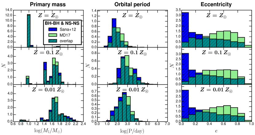
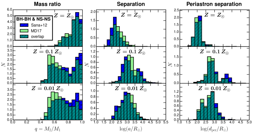
Figure 4: Birth distributions of initial ZAMS binary parameters of the progenitors of BH-BH and NS-NS mergers. The histograms are normalized to unity for an easier comparison. NS-NS mergers dominate at $Z={\leavevmode\nobreak\ Z}_{\odot}$ (upper panel) while BH-BH mergers dominate at $Z=0.1{\leavevmode\nobreak\ Z}_{\odot}$ and $Z=0.01{\leavevmode\nobreak\ Z}_{\odot}$ (lower panels).

Table 1: Comparison of the formation efficiencies per unit of star-forming mass of CBM: BH-BH, BH-NS, and NS-NS between the two models with different initial distributions: either Sana et al. (2012; , old) or MD17(new). The comparison is made at three different metallicities. No metallicity-dependence for the IMF is assumed here. We indicate in bold text the dominant metallicity (out of the three showed here) for the formation of each type of the double compact mergers.

	Formation efficiency
Metallicity	$X_{\rm CBM}$ $(M_{\odot}^{-1})$		Relative
merger type	Sana+12	MD17	MD17 / Sana
	(model M10)	(model I1)
$Z=Z_{\odot}$
NS-NS	$\mathbf{8.3\times 10^{-6}}$	$\mathbf{3.8\times 10^{-6}}$	$0.46$
BH-NS	$9.0\times 10^{-8}$	$1.1\times 10^{-7}$	$1.22$
BH-BH	$3.5\times 10^{-7}$	$1.5\times 10^{-7}$	$0.43$
$Z=0.1{\leavevmode\nobreak\ Z}_{\odot}$
NS-NS	$1.75\times 10^{-6}$	$1.0\times 10^{-6}$	$0.57$
BH-NS	$\mathbf{3.0\times 10^{-6}}$	$\mathbf{1.2\times 10^{-6}}$	$0.4$
BH-BH	$2.1\times 10^{-5}$	$8.4\times 10^{-6}$	$0.4$
$Z=0.01{\leavevmode\nobreak\ Z}_{\odot}$
NS-NS	$1.7\times 10^{-6}$	$1.2\times 10^{-6}$	$0.71$
BH-NS	$9.6\times 10^{-7}$	$3.6\times 10^{-7}$	$0.38$
BH-BH	$\mathbf{5.3\times 10^{-5}}$	$\mathbf{2.9\times 10^{-5}}$	$0.55$

4.1.1 Progenitors of BH-BH and NS-NS mergers

In Fig. 4, we show the birth properties of systems that evolve to form BH-BH and NS-NS mergers. We only include double compact binaries that are expected to merge within the Hubble time. The histograms are normalized to unity for an easier comparison; see Table 4 for the relative formation efficiencies.

Primary masses: The distributions of primary masses are noticeably different in different metallicities. The peak around $10{\leavevmode\nobreak\ M}_{\odot}$ at $Z=0.02$ corresponds to NS-NS progenitors, which are the dominant type of CBM at solar metallicity. At $Z=0.002$ the formation of BH-BH begins to dominate and happens for primary masses $M_{1}>20{\leavevmode\nobreak\ M}_{\odot}$, peaking around $25$ and $45{\leavevmode\nobreak\ M}_{\odot}$. This bimodal shape is a direct consequence of the bimodal distribution of CO core masses $M_{\rm CO}$ of supernova progenitors expected to undergo a direct BH formation. In the rapid supernova engine we adopted (Fryer et al. 2012), BHs receive no natal kick on formation if $M_{\rm CO}$ is either between $6$ and $7{\leavevmode\nobreak\ M}_{\odot}$ or above $11{\leavevmode\nobreak\ M}_{\odot}$ (see their Eqn. 16). At $Z=0.01{\leavevmode\nobreak\ Z}_{\odot}$ the higher mass peak corresponding to $M_{\rm CO}>11{\leavevmode\nobreak\ M}_{\odot}$ dominates.

The differences between the new and old initial distributions are very small. The NS-NS as well as lower mass BH-BH corresponding to $M_{\rm CO}$ = 6$-$7${\leavevmode\nobreak\ M}_{\odot}$ are most preferably formed from systems with very high initial mass ratios $q>0.8$, which is why there is relatively less of such systems in the simulations with MD17 initial conditions.

Orbital periods, eccentricities, and periastron separations: The new initial binary period distribution of MD17 is in general very similar in shape to that proposed by Sana et al. (2012) in the crucial range of ${\rm log}\,P\,{\rm(days)}$ between $2$ and $4$ (especially for systems with massive primaries $\sim$ $30{\leavevmode\nobreak\ M}_{\odot}$; see Fig. 1). However, there is a noticeable shift towards larger periods (and separations) among compact binary merger progenitors in the new simulations. This can be explained in connection with the eccentricity distribution of these systems. In the case of MD17 the eccentricity distribution is slightly skewed towards $e>0.5$, which is very different from that of Sana et al. (2012) showing a strong preference for nearly circular orbits. As a result the periastron separation distributions in the new and old simulations are very similar. This showcases the fact that the pericentre separation $d_{\rm per}$ determines the evolutionary path of a binary with given component masses and decides whether or not it will form a compact binary merger. In the evolutionary channel involving a CE phase, only a fixed range of $d_{\rm per}$, that is independent of the choice of initial properties, results in the formation of CBM.

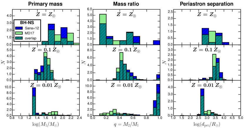
Figure 5: Birth distributions of initial ZAMS binary parameters of the progenitors of BH-NS mergers. The histograms are normalized to unity for an easier comparison. We note that the upper panels ($Z={\leavevmode\nobreak\ Z}_{\odot}$) are made based on a very small number of systems ($<20$) that form in solar metallicity.

At $Z={\leavevmode\nobreak\ Z}_{\odot}$, where the formation of NS-NS dominates, the periastron separations are centred around $\sim$ $100{\leavevmode\nobreak\ R}_{\odot}$. At $Z=0.1{\leavevmode\nobreak\ Z}_{\odot}$ BH-BH become dominant and shift the $d_{\rm per}$ distribution towards higher values of over $\sim$ $100{\leavevmode\nobreak\ R}_{\odot}$. At this metallicity the distribution is clearly bimodal with peaks around $\sim$ $750{\leavevmode\nobreak\ R}_{\odot}$ and $\sim$ $4000{\leavevmode\nobreak\ R}_{\odot}$. This comes from the fact that at $Z\sim 0.1{\leavevmode\nobreak\ Z}_{\odot}$ there are two relevant formation channels of merging BH-BH: the dominant channel ($\sim$70% of the systems), in which there is only one CE phase taking place after the first BH has already formed (the peak at $d_{\rm per}$ $\sim$ $750{\leavevmode\nobreak\ R}_{\odot}$); and another channel ($\sim$20% of the systems), in which there are two CE phases, one before each BH formation. The systems originating from the latter channel are those responsible for the second peak at $d_{\rm per}$ $\sim$ $4000{\leavevmode\nobreak\ R}_{\odot}$. These systems need to have larger initial $d_{\rm per}$ to prevent any RLOF during the HG evolutionary stage of the primary; we note that we do not allow for the CE phase from HG donors. Instead, the primary needs to initiate a RLOF and the CE phase later during the core helium burning phase. This channel becomes ineffective in our simulations for extremely low metallicities ($Z\lesssim 0.0005$), where stars do not increase their radii sufficiently after the HG stage. For that reason at $Z=0.01{\leavevmode\nobreak\ Z}_{\odot}$, the $d_{\rm per}$ distribution is no longer clearly bimodal. It is also slightly shifted towards smaller separations with respect to the distribution at $Z=0.1{\leavevmode\nobreak\ Z}_{\odot}$, again because of smaller sizes of the stars. Overall, the BH-BH formation channel involving two different CE phases is only relevant (i.e. at least 5% of all the BH-BH formed this way) at metallicity range $Z$  = $0.0005$ - $0.004$, contributing up to at most $\sim$ 22% of the BH-BH formation at metallicity $Z$ $\approx$ $0.0025$.

We note that the secondary peak in pericentre separations around $\sim$ $4000{\leavevmode\nobreak\ R}_{\odot}$ at $Z=0.1{\leavevmode\nobreak\ Z}_{\odot}$ is noticeably smaller in the simulations with the new initial distributions. This is because of the fact that, according to the multiplicity statistics of MD17, the number of inner binaries with massive primaries ($\gtrsim 30{\leavevmode\nobreak\ M}_{\odot}$) having orbital periods of about ${\rm log}\,P\,{\rm(days)}\approx 3.5$ to $4.0$ is smaller with respect to the old distributions of Sana et al. (2012); see Fig. 1.

Mass ratios: Merging NS-NS and BH-BH in our simulations originate almost exclusively from binaries with high mass ratios: $q_{\rm NS-NS}\gtrsim 0.6$ and $q_{\rm BH-BH}\gtrsim 0.5$, respectively (at $Z=0.1{\leavevmode\nobreak\ Z}_{\odot}$ the systems with initial $q<0.5$ are all BH-NS). The initial mass ratio distribution of Sana et al. (2012) is flat in $q$. Meanwhile, the new results of MD17 include a distribution decreasing quickly with $q$ (see Fig. 3). This is reflected in the changes of the mass ratio distribution of CBM progenitors, which are slightly shifted towards $q$ $\sim$ 0.5 at $Z=0.1{\leavevmode\nobreak\ Z}_{\odot}$ and $Z=0.01{\leavevmode\nobreak\ Z}_{\odot}$ in the new simulations.

4.1.2 Progenitors and formation of BH-NS mergers

In Fig. 5, we show the birth properties of systems that evolve to form BH-NS mergers. This time, for simplicity, we focus only on the three most important parameters: primary mass, mass ratio, and periastron separation.

The formation of BH-NS mergers is very different in the three different metallicites shown: ${\leavevmode\nobreak\ Z}_{\odot}$, $0.1{\leavevmode\nobreak\ Z}_{\odot}$, and $0.01{\leavevmode\nobreak\ Z}_{\odot}$. In the solar metallicity there are hardly any BH-NS systems formed. The histograms for $Z={\leavevmode\nobreak\ Z}_{\odot}$ are based on only around a dozen binaries, and, as a result, these histograms are not very meaningful. The reason why the BH-NS formation is so ineffective in our simulations at solar metallicity is that the stars with $Z={\leavevmode\nobreak\ Z}_{\odot}$ already expand to their nearly maximum radius during the HG phase. This means that, in the majority of cases, the RLOF is initiated from the primary while it is a HG star. Because BH-NS systems typically originate from binaries with relatively small initial mass ratios of $q\lesssim 0.6$, then, according to the standard StarTrack criteria, such a mass transfer would most likely be flagged as unstable, leading to a CE phase from a HG donor. In this work, we decided to not follow the evolution of such systems (see Sect. 3.1 for more details).

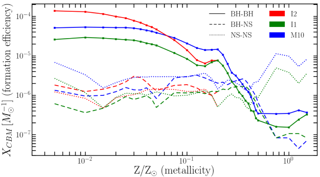
Figure 6: Formation efficiency (i.e. number of systems formed per unit of star-forming mass, $X_{\rm CBM}\;({\leavevmode\nobreak\ M}_{\odot}^{-1})=N_{\rm CBM}/M_{\rm sim}$) of different types of CBM at different metallicities. We compute a grid of 32 different metallicities (indicated with filled squares at the BH-BH curves), ranging from $0.005{\leavevmode\nobreak\ Z}_{\odot}$ to $1.5{\leavevmode\nobreak\ Z}_{\odot}$. We indicate three different models: M10 in blue (initial distributions of Sana et al. 2012), I1 in green (initial distributions of MD17) and I2 in red (same as I1 but with a top-heavy IMF at low metallicities; see Eq. 2). We note that model I2 is only different from I1 at $Z<0.004=0.2{\leavevmode\nobreak\ Z}_{\odot}$.

At subsolar metallicity $Z=0.1{\leavevmode\nobreak\ Z}_{\odot}$ the formation of BH-NS mergers is much more effective, and the initial distributions are representative for the majority of BH-NS mergers formed across all of the 32 metallicites we compute. The primary expands much more after the HG phase than in the case of solar metallicity (Fig. 2 of Belczynski et al. 2010b) and, as a core-helium burning giant with a convective envelope, initiates an unstable RLOF and a CE phase. After the BH formation, the secondary eventually evolves off the MS, expands, and initiates a second CE episode. As a result, the binary is very close, the natal kick velocity gained by a newly formed NS does not disrupt the system and the binary merges within the Hubble time. We note that this is the exact same evolutionary route (i.e. two CE phases) that also operates in the case of BH-BH mergers in intermediate metallicites $Z$  = $0.0005$–$0.004$; see the paragraph on orbital periods in Section 4.1.1.

The distribution of primary masses at $Z=0.1{\leavevmode\nobreak\ Z}_{\odot}$ is slightly shifted towards lower values (peak at $\sim 40{\leavevmode\nobreak\ M}_{\odot}$) with respect to the same distribution for BH-BH progenitors (peak at $\sim 50{\leavevmode\nobreak\ M}_{\odot}$). The dominant range of mass ratios is between $0.3$ and $0.6$ (the contribution from $q>0.95$ is described below). In the simulation with the updated initial distributions from MD17, the mass ratio distribution is slightly shifted towards smaller values. This, in turn, causes a small shift towards higher $M_{1}$ values, so that the secondary mass distribution (not explicitly shown here) stays roughly the same. The optimal periastron separation is about $3000{\leavevmode\nobreak\ R}_{\odot}$ similar to the case of BH-BH mergers evolving through the same channel involving two CE phases; see the right peak in the periastron separation distribution for $Z=0.1{\leavevmode\nobreak\ Z}_{\odot}$ in Fig. 4. We note that in the case of new simulations with the initial conditions of MD17 there are fewer binaries with initial periods above ${\rm log}\,P\,{\rm(days)}\approx 3.5$ with respect to the old distributions of Sana et al. (2012), which is why the peak in the periastron separations is slightly shifted towards smaller values (also similarly to the BH-BH case at $Z=0.1{\leavevmode\nobreak\ Z}_{\odot}$).

In the case of very low metallicities (such as $Z=0.01{\leavevmode\nobreak\ Z}_{\odot}$) the main formation channel of BH-NS mergers described above is no longer efficient. This is because the lower the metallicity the more massive the BHs formed. For comparison, the least massive BHs in our simulations are of about $5.5{\leavevmode\nobreak\ M}_{\odot}$ at $Z=0.1{\leavevmode\nobreak\ Z}_{\odot}$ and about $7.0{\leavevmode\nobreak\ M}_{\odot}$ at metallicity $Z=0.01{\leavevmode\nobreak\ Z}_{\odot}$. As a result, at $Z=0.01{\leavevmode\nobreak\ Z}_{\odot}$, the mass ratio of the components at the point when the secondary expands and initiates a RLOF is not sufficiently high to cause an unstable mass transfer and a CE phase.

At $Z=0.01{\leavevmode\nobreak\ Z}_{\odot}$ another formation channel dominates, which is also present, yet not so important at higher metallicities. This channel involves binaries with a mass ratio close to unity ($q\gtrsim 0.9$), comprised of stars with masses that are close to the threshold between the NS and BH formation ($M\sim 20{\leavevmode\nobreak\ M}_{\odot}$). Because the binary components have similar masses, the secondary evolves transfer between the two core-helium burning stars, which reverses the mass ratio of the components. The primary eventually collapses to form a BH in a direct event with no mass eject and no natal kick. The ‘Rapid’ BH formation model of Fryer et al. (2012) predicts a 100% mass fallback for the least massive BH progenitors with CO core masses between 6 and 7${\leavevmode\nobreak\ M}_{\odot}$; see their Eq. 16. The rejuvenated secondary continues to expand and initiates a second RLOF. This time the mass ratio is lower and the mass transfer becomes unstable, leading to a CE phase. The binary becomes close enough to survive the supernova and NS formation, and later becomes a BH-NS merger. This scenario requires a specific range of initial binary parameters and is much less effective than the more standard evolutionary route dominating the BH-NS formation at intermediate metallicities.

4.2 Formation of compact binary mergers across metallicity

In Fig. 6 we show the relation between the formation efficiency $X_{\rm CBM}\;({\leavevmode\nobreak\ M}_{\odot}^{-1})$ and metellicity for different types of CBM. We note that similar trends were obtained recently by Giacobbo & Mapelli (2018). It is evident that the formation of BH-BH mergers becomes most effective at low metallicities $Z\lesssim 0.1{\leavevmode\nobreak\ Z}_{\odot}$. This is a well-known result (e.g. Belczynski et al. 2010b; Dominik et al. 2012; Eldridge & Stanway 2016; Belczynski et al. 2016b; Mapelli et al. 2017; Giacobbo & Mapelli 2018) for mainly two reasons: first, the fact that at lower metallicities the BH progenitors are relatively more massive and, therefore, more BHs are formed through direct collapse with zero natal kick, and second there is a higher chance for a CE event to be initiated by a core-helium burning donor, rather than by a HG donor, because of smaller radii of HG stars (Fig. 2 of Belczynski et al. 2010b).

According to stellar tracks from Hurley et al. (2000), at metallicities close to the solar $Z\simeq 0.02$, there is only a small range of separations at which a mass transfer from core-helium burning donors of $>20{\leavevmode\nobreak\ M}_{\odot}$ is initiated. Much more likely, the giant causes a RLOF earlier during its rapid HG evolution, in which case we choose to not allow for a CE evolution. Apart from strong stellar winds, this is what suppresses the formation of BH-BH and BH-NS compact binaries at metallicities close to the solar $Z\simeq 0.02$ in our simulations.

The formation efficiency of BH-NS mergers $X_{\rm BHNS}\;({\leavevmode\nobreak\ M}_{\odot}^{-1})$ does not increase in a similar fashion as $X_{\rm BHBH}\;({\leavevmode\nobreak\ M}_{\odot}^{-1})$ does at very low metallicities. There are two major factors at play. The main formation channel of BH-NS involving two CE phases becomes less effective in very low metallicities (Sect. 4.1.2). Additionally, natal kicks for NSs formed in core collapse are significant even at very low metallicities.

The formation of NS-NS mergers is much less metallicity-dependent, as was similarly found by Giacobbo & Mapelli (2018). It is slightly more efficient at metallicities similar to solar ($Z\simeq 0.02$) than it is at lower metallicities $Z\lesssim 0.005$. There is no one single reason for this behaviour, and it is most likely a combination of small effects such as different radii and different wind mass loss rates of stars with different metallicities. We thus consider this result to be much less robust than the increasing formation efficiency of BH-BH mergers towards lower metallicity.

The updated initial binary distributions of MD17 (green lines, I1) result in smaller formation efficiencies of CBM across all the metallicities with respect to the previously adopted distributions of Sana et al. (2012; blue lines, M10). The only exception is the case of BH-NS mergers at $Z\approx{\leavevmode\nobreak\ Z}_{\odot}$, where the formation efficiency $X_{\rm BHNS}\;({\leavevmode\nobreak\ M}_{\odot}^{-1})$ is at its lowest and there are few such systems in our simulations (fewer than 20). On the other hand, the inclusion of a top-heavy IMF for $Z<0.004=0.2{\leavevmode\nobreak\ Z}_{\odot}$ (red lines, I2) significantly increases the formation efficiency of BH-BH and BH-NS mergers by up to nearly an order of magnitude for the lowest $Z=0.0001=0.005{\leavevmode\nobreak\ Z}_{\odot}$ in the case of BH-BH. The NS-NS mergers originate from binaries with less massive primaries, which is why there is little change between models I1 and I2 in this case.

5 Merger rates and LIGO/Virgo predictions

5.1 Source-frame merger rate density

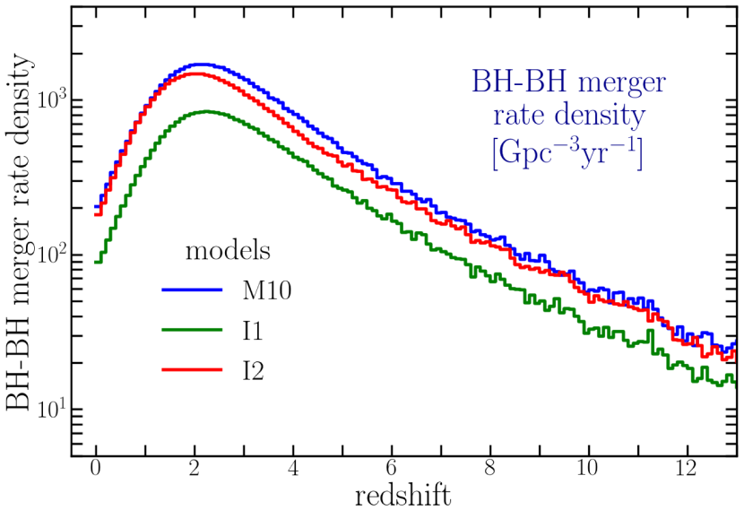
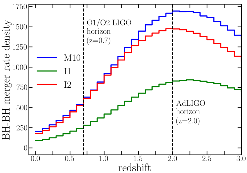
Figure 7: Source frame BH-BH merger rate density $Gpc^{-3}\,yr^{-1}$ as a function of redshift for our three models: M10 (binary distributions of Sana et al. (2012)), I1 (binary distributions of MD17) , and I2 (same as I1 but with a metallicity-dependent IMF). Upper panel: the peak around $z\approx 2$ in all the models corresponds to the maximum in the SFR (see text). Lower panel: the range of redshifts accessible with the current and future sensitivity of LIGO detectors. We indicate the horizon redshifts for observation of an optimally inclined BH-BH merger with a total mass of $\sim 80{\leavevmode\nobreak\ M}_{\odot}$ (roughly the most massive systems in our simulations) for the sensitivities of O1 and O2 observing runs , and for the Advanced LIGO (AdLIGO). The detection distances for NS-NS mergers (Chen et al. 2017) were about $d_{\rm NSNS}=70$ Mpc for O1 and O2 sensitivity (Abbott et al. 2018). The local BH-BH merger rate density (within $z<0.02$) in our models are about 203 (M10), 89 (I1), and 181 ${\rm\leavevmode\nobreak\ Gpc}^{-3}{\rm\leavevmode\nobreak\ yr}^{-1}$ (I2). The current limits imposed by the existing LIGO detections are 12$-$219${\rm\leavevmode\nobreak\ Gpc}^{-3}{\rm\leavevmode\nobreak\ yr}^{-1}$ (Abbott et al. 2017a).

In Fig. 7 we show the source frame BH-BH merger rate density ($Gpc^{-3}\,yr^{-1}$) as a function of redshift for our three models. We note that the results for M10 are also corrected with respect to Belczynski et al. (2016a) for a typo in the calculation of simulation normalization, yielding a small net decrease of merger rates by a factor of 0.926 (Sect. 3.4).

The behaviour of the merger rate density relation with redshift (upper plot) closely resembles the star formation history (Madau & Dickinson 2014)and peaks around $z\approx 2$. This results from the fact that the distribution of merger delay times of close BH-BH binaries follows a power-law $\propto t_{\rm del}^{-1}$ (Dominik et al. 2012; Belczynski et al. 2016b), and most of the systems merge relatively shortly after their formation (a few hundred Myr). We note that the maximum of BH-BH merger rate density in model I2 is very slightly ($\Delta z\approx 0.2$) shifted towards smaller redshifts. This is because in this variation, at each redshift, we assume a different IMF based on the mean metallicity at that redshift, and consequently apply the adequate IMF-SFR correction factor (see Appendix A for details). As a result, the location of the SFR maximum is slightly different.

The lower panel shows the range of redshifts up to $z=3.0$. We also indicate the horizon redshifts for observation of an optimally inclined BH-BH merger with a total mass of $\sim 80{\leavevmode\nobreak\ M}_{\odot}$ (roughly the most massive systems in our simulations) for the sensitivities of O1 and O2 observing runs ($z_{\rm horizon}\approx 0.7$), and for the design sensitivity of Advanced LIGO ($z_{\rm horizon}\approx 2.0$; Abbott et al. 2018). For comparison, the detection distances for NS-NS mergers ($d_{\rm NSNS}$; i.e. the radius of a sphere with an equal volume to the peanut-shaped LIGO response function; see Chen et al. 2017) were about $d_{\rm NSNS}=70$ Mpc for O1 and O2 sensitivity. The local BH-BH merger rate density (within $z<0.02$) in our models are about 203 (M10), 89 (I1), and 181 ${\rm\leavevmode\nobreak\ Gpc}^{-3}{\rm\leavevmode\nobreak\ yr}^{-1}$ (I2), which are all within the most up-to-date range determined by the existing LIGO detections (12$-$219${\rm\leavevmode\nobreak\ Gpc}^{-3}{\rm\leavevmode\nobreak\ yr}^{-1}$ Abbott et al. 2017a).

5.2 LIGO/Virgo detection rates

In Table 5, we summarize our predictions for the local (i.e. within $z<0.02$) merger rate densities, detection rates ($R_{\rm det}\,yr^{-1}$) with the sensitivity of O1/O2 LIGO/Virgo observing runs, and corresponding numbers of detections assuming 120 days of coincident data acquisition. The inclusion of the updated initial MS binary distributions of MD17 (model I1) has led to a decrease in both the local BH-BH merger rate density and the detection rate during O2 by a factor of $\sim$2.3 (with respect to model M10). The assumption of a metallicity-dependent IMF (model I2, see Eq. 2), on the other hand, causes an increase in the local BH-BH merger rate density by a factor of $\sim 2$, and an increase in the O2 detection rate by a larger factor of $\sim 2.5$ (with respect to model I1). The difference between these two factors arises from the fact that the top-heavy IMF for low metallicities assumed in I2 favours more massive BHs, which are easier to detect. We discuss the comparison of our results with LIGO/Virgo detection rates in Sect. 6.4.

5.3 Metallicity distribution of BH-BH progenitors

In Fig. 8, we show the metallicity distributions of different types of CBM weighted by their detection rates with O1/O2 sensitivity. In the case of BH-BH mergers, the huge preference for very low metallicities ($Z\lesssim 0.001=0.05{\leavevmode\nobreak\ Z}_{\odot}$) with respect to metallicities close to solar ($Z\gtrsim 0.01=0.5{\leavevmode\nobreak\ Z}_{\odot}$) is already present when looking at the formation efficiencies across $Z$ alone (see Fig. 6). At that stage, which does not account for any cosmological calculations yet (i.e. SFR, cosmic metallicity distribution, BH-BH merger delay times), there are about 2 orders of magnitude more BH-BH mergers formed with low $Z\lesssim 0.001$ compared to $Z\sim{\leavevmode\nobreak\ Z}_{\odot}$ (solely due to binary evolution effects). Notably, this difference grows much higher in the detector frame, with the values of d$R_{\rm det}/$d$Z$ being about 4 order of magnitude larger for $Z\lesssim 0.001$ than for $Z\sim{\leavevmode\nobreak\ Z}_{\odot}$. This is a combination of two effects. First, at low metallicities BHs are born more massive and their mergers are easier to detect with the LIGO/Virgo sensitivity. Second, in our approach to population synthesis on cosmological scales (Sect. 3.2) the metallicity distribution of stars forming at redshifts around the maximum of the cosmic SFR at $z\approx 2$, from which most of the BH-BH merger progenitors originates (see Fig. 2 of B16), is centred at $Z<0.1{\leavevmode\nobreak\ Z}_{\odot}$ (see Fig. 6 of Extended Data of B16).

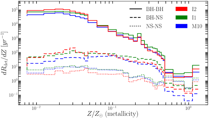
Figure 8: Detector-frame distribution of metallicities of BH-BH, BH-NS, and NS-NS merger progenitors. More than 90% of BH-BH merger detections in all our models are systems formed with metallicites lower than 10% of the solar metallicity, i.e. $Z<0.1{\leavevmode\nobreak\ Z}_{\odot}$. Such a strong dependence of compact binary merger formation with metallicity (see also Fig. 6), especially in the case of BH-BH systems, indicates the significance of SFRs at different metallicites across the Universe for the compact binary merger rates (see discussion in Sect. 6.3).

Table 2: Merger rate densities and detection rates for the LIGO/Virgo O2 run sensitivity for three models: M10 (initial binary distributions from Sana et al. (2012)), I1 (updated distributions from MD17), and I2 (I1 plus top-heavy IMF for low metallicities from Marks et al. (2012)).

Model	Rate density	O2 rate	O2
merger type	[Gpc-3 yr-1]	[yr-1]	[120 days]
M10
NS-NS	68.2	0.09	0.03
BH-NS	26.7	0.42	0.22
BH-BH	203	111.6	36.7
I1
NS-NS	25.9	0.03	0.01
BH-NS	13.3	0.25	0.08
BH-BH	88.8	48.6	16
I2
NS-NS	24.4	0.03	0.01
BH-NS	16.5	0.38	0.13
BH-BH	181	122.7	40.3

6 Discussion

6.1 Understanding the impact of the new initial distributions

Within the classical binary evolution scenario, our predictions for the merger rates of double compact objects based on the updated initial MS binary parameters from MD17 are $\sim 2-2.5$ times smaller than the results previously obtained by dMB15 and B16 from the distributions of Sana et al. (2012). This can be explained by looking at the differences between the two distributions within the areas of the parameter space that are most relevant for the formation of double compact object mergers. Let us first take a look at BH-BH and NS-NS progenitors.

(i) In agreement with dMB15, we find that the majority of BH-BH and NS-NS mergers originate from binaries with initial periods within ${\rm log}\,P\,{\rm(days)}$ = 2$-$4. The fraction of primaries residing in such systems is about F_logP=2-4;bin = 28% in the case of Sana et al. (2012) distributions. Meanwhile, this value is higher by about $\sim 1.35$ in the case of statistics obtained by MD17 (Fig. 1): i.e. F_logP=2-4;bin = 37% for $M_{1}$ = $8{\leavevmode\nobreak\ M}_{\odot}$ primaries, and F_logP=2-4;bin = 40% for $M_{1}$ = $30{\leavevmode\nobreak\ M}_{\odot}$ primaries (regimes for NS-NS and BH-BH progenitors, respectively).

(ii) The eccentricity distribution based on the Sana et al. (2012) sample is skewed towards lower values with $<$ $e$ $>$ = 0.3 compared to the statistics reported by MD17 with $<$ $e$ $>$ = 0.6 in the case of massive binaries (Fig. 2). The progenitors of CBM derive from binaries with periastron separations log $d_{\rm per}$ (${\leavevmode\nobreak\ R}_{\odot}$) = 2$-$3.5, depending slightly on metallicity and the exact formation channel. By increasing the average initial eccentricity from $<$ $e$ $>$ = 0.3 to 0.6, then the average orbital separation of the progenitors increases by a factor of (1$-$0.3)/(1$-$0.6) = 1.75. This corresponds to a shift in logarithmic orbital period of $\Delta$log$P$ $\approx$ 0.2. Considering the progenitors derive from a broad parameter space of orbital periods ${\rm log}\,P\,{\rm(days)}$ = 2$-$4, a slight shift of $\Delta$log$P$ $\approx$ 0.2 due to the updated eccentricity distribution does not affect the predicted rates of compact object mergers.

(iii) Similar to dMB15, we find that nearly all BH-BH and NS-NS mergers derive from initial MS binaries with mass ratios $q$ = 0.5$-$1.0. According to the old mass-ratio distribution from Sana et al. (2012), $\approx$55% of early-type binaries have mass ratios across this interval. According to the updated period-dependent mass-ratio distribution of MD17, however, only (17-28)% of massive binaries with ${\rm log}\,P\,{\rm(days)}$ = 2$-$4 have mass ratios $q$ = 0.5$-$1.0, which results in about $\sim$2.0$-$3.2 times fewer potential BH-BH and NS-NS merger progenitors.

Altogether, the new mass ratio distribution that is shifted towards smaller values with respect to the old distribution (iii) is the most significant update in the context of BH-BH and NS-NS mergers, and the differences between period distributions are of secondary importance (i). Based on the estimates presented above, we could expect that there should be roughly between 1.5 and 2.4 fewer BH-BH and NS-NS mergers in the updated simulations. This explains the results of our computations (see tables 4 and 5).

In the case of BH-NS mergers, the binary parameters of their progenitors depend strongly on metallicity (Fig. 5). Around solar metallicity, there are few to no BH-NS systems formed and our sample is not statistically significant. At subsolar metallicities of $\sim 0.1{\leavevmode\nobreak\ Z}_{\odot}$, the main formation channel involves two CE phases, and this channel dominates when summed across all metallicities. It requires the initial mass ratios between 0.3 and 0.6 (peaking around 0.4) and, more importantly, pericentre separations of log $d_{\rm per}$ (${\leavevmode\nobreak\ R}_{\odot}$) = 3.2$-$4, preferably over 3.5. The updated initial distributions predict fewer massive binaries this wide. Additionally, in most cases the NS is formed from a star with mass at the higher end of the mass range of NS progenitors ($15\lesssim M_{2}/{\leavevmode\nobreak\ M}_{\odot}\lesssim 22$), which helps to produce a high enough mass ratio at a BH-MS binary stage, so that a dynamically unstable mass transfer occurs and a CE phase is triggered. The shift towards smaller mass ratios in the updated distributions causes a corresponding shift towards slightly more massive primaries. This additionally decreases the BH-NS formation efficiency due to a declining slope of the IMF.

At very low $Z$ $\sim$ $0.01{\leavevmode\nobreak\ Z}_{\odot}$, the dominant formation channel involves binaries with components of initially similar masses that evolve into double-giant systems and experience a stable mass transfer instead of the first CE (Sect. 4.1.2). The requirement of $q$ ¿ 0.9 means that there are about three times fewer potential progenitors for this channel in the updated distributions. With all the metallicities combined, all the factors described above result in the merger rate of BH-NS systems being about two times smaller in the new simulations (Table 5).

6.2 Small impact of a top-heavy IMF

The uncertainty in the IMF is often considered to have a substantial impact on the compact binary merger rates, by a factor of a few (dMB15) up to an order of magnitude (see Fig. 20 of Kruckow et al. 2018). One could thus expect that the top-heavy IMF for low metallicities ($Z<0.2{\leavevmode\nobreak\ Z}_{\odot}$; see Eqn. 2) we implemented in model I2 would result in a significant increase of BH-BH merger rates. According to Fig. 8, the vast majority of BH-BH mergers detectable with LIGO/Virgo were formed in $Z<0.1{\leavevmode\nobreak\ Z}_{\odot}$ metallicity environments. In model I2, the IMF power-law exponent for massive stars is $\alpha_{3}\approx 2.07$ for $Z=0.1{\leavevmode\nobreak\ Z}_{\odot}$ decreasing down to as low as $\alpha_{3}\approx 1.31$ for $Z=0.01{\leavevmode\nobreak\ Z}_{\odot}$. For a fixed amount of stellar mass formed (i.e. fixed SFR) and with respect to the standard value $\alpha_{3}=2.3$ as in models M10 and I1, this would correspond to an increase in the number of primaries within $\rm M_{1}$ = 45$-$55 ${\leavevmode\nobreak\ M}_{\odot}$ (highest bin in the primary mass distribution of BH-BH progenitors, Fig. 4) by a factor of about $\sim 2.2$ at $Z=0.1{\leavevmode\nobreak\ Z}_{\odot}$ and $\sim 5$ at $Z=0.01{\leavevmode\nobreak\ Z}_{\odot}$. Meanwhile, the merger rate density of BH-BH in model I2 (with a top-heavy IMF) is higher than in model I1 by only a factor of $\sim 2$.

This showcases the significance of keeping the consistency between an adopted cosmic SFR and an assumed IMF. Because the cosmic SFR is measured based on UV observations (Madau & Dickinson 2014), we normalize our simulations in such a way that the total amount of UV light at $\rm 1500\AA$ stays roughly constant, irrespective of the assumed IMF (see Appendix A). As most of the UV light is produced by massive stars, a top-heavy IMF is characterized by a higher UV luminosity per unit of stellar mass formed $\mathcal{U}\;({\leavevmode\nobreak\ M}_{\odot}^{-1})$ and must result in a rescaling of the SFR to a smaller value. A smaller SFR means fewer stars formed, which counteracts the fact that with a top-heavy IMF a higher fraction of these stars are massive. A similar but inverted argument could be made for a top-light IMF (i.e. $\alpha_{3}>2.3$). Thus, the total number of massive stars formed stays roughly constant irrespective of the IMF variations, as it is constrained by the UV observations.

We show this quantitatively in Fig. 9, where, as a function of $\alpha_{3}$, we plot the relative number $\mathcal{R}(\alpha_{3})$ of stars formed in a given mass bin $M_{\rm low}$-$M_{\rm high}$ (e.g. between 8 and 13 ${\leavevmode\nobreak\ M}_{\odot}$, and so on) defined as

$$\mathcal{R}(\alpha_{3})=\frac{M_{\rm total;1}(\alpha_{3})\times\int_{M_{\rm low}}^{M_{\rm high}}\xi(\alpha_{3},M)dM}{M_{\rm total;2}(\alpha_{3}=2.3)\times\int_{M_{\rm low}}^{M_{\rm high}}\xi(\alpha_{3}=2.3,M)dM},$$ (6)

where $\xi(\alpha_{3},M)$ is a Kroupa-like IMF in the form given by Eq. 1 for which we vary the high-mass slope $\alpha_{3}$, and $M_{\rm total;1}$ and $M_{\rm total;2}$ are the total amounts of stellar mass formed in models with different IMFs. The IMFs are normalized to unity, i.e. $\int_{0.08}^{150}\xi(\alpha_{3},M)dM=1.0$ for any slope $\alpha_{3}$. The upper panel represents simulations normalized to a fixed amount of stellar mass formed, irrespective of the IMF (the usually made assumption), so $M_{\rm total;1}=M_{\rm total;2}$. The lower panel, in turn, assumes a fixed UV luminosity of a star-forming population, so that $M_{\rm total;1}\times\mathcal{U}(\alpha_{3})=M_{\rm total;2}\times\mathcal{U}(\alpha_{3}=2.3)$. The amount of UV light per unit of star-forming mass $\mathcal{U}\;({\leavevmode\nobreak\ M}_{\odot}^{-1})$ is inversely proportional to $\mathcal{K}$ coefficients in Eq. 7 and Table 3.

We note that although the relative number of primaries does not change by more than a factor of $\sim 2$ in any of the mass ranges and IMFs shown, the ratio of progenitors of massive BH-BH to NS-NS mergers changes more significantly.

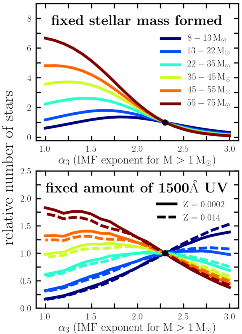
Figure 9: Relative numbers of massive stars $\mathcal{R}$ formed within multiple initial mass ranges as a function of power-law exponent $\alpha_{3}$ for the high-mass IMF component ($\rm M>1\,M_{\odot}$). See eq. 6 for the exact definition of $\mathcal{R}$. Upper panel: the same SFR, irrespective of the IMF changes. The number of stars is thus calculated with respect to a fixed stellar mass formed. Lower panel: SFR corrected for the IMF changes (see Eqn. 5). The number of stars is thus calculated with respect to a fixed amount of UV radiation at $1500\AA$ wavelength that is constrained by the observations (Madau & Dickinson 2014).

6.3 Population synthesis on cosmological scales

The discovery of GW150914 revealed the existence of stellar BHs with masses of 30 $-$ 40${\leavevmode\nobreak\ M}_{\odot}$ (Abbott et al. 2016c). Black holes this massive are only expected to form from low-metallicity stars $Z/{\leavevmode\nobreak\ Z}_{\odot}\lesssim 0.3$ (Belczynski et al. 2010a), and this conclusion is strengthened by a recent update to Wolf-Rayet star winds (Vink 2017). Additionally, Fig. 6 shows that the formation efficiency of BH-BH mergers is very strongly dependent on metallicity. For that reason, predictions for the rates of such events are sensitive to the applied distribution of metallicity of star formation throughout the Universe and they cannot be made by simply extrapolating results for a Milky Way-like galaxy, as still done by some authors.

We have adopted the mean metallicity-redshift relation from the chemical evolution model of Madau & Dickinson (2014; see Eqn. 4) with the level increased by 0.5 dex and with a Gaussian spread of $\sigma$ = 0.5 dex, and used this relation to weight the contributions from different metallicities to the SFR at different redshifts. This cosmological information, combined with the LIGO/Virgo sensitivity, allowed us to transform our simulated CBM into detector-frame predictions.

However, the mean metallicity of the Universe (defined as the total mass of heavy elements ever produced per mass of baryons in the Universe) in general does not equal the mean metallicity of star formation at a given redshift. This simplification is a caveat of our model to keep in mind. The mean metallicity at which star formation takes place is likely higher, since the highest SFRs are revealed by massive galaxies (Lara-López et al. 2013), which are also relatively metal rich (e.g. Tremonti et al. 2004). Low-metallicity star formation in the local Universe, on the other hand, occurs mostly in low-mass dwarf galaxies (Andrews & Martini 2013), which have relatively little star formation (Boogaard et al. 2018). For that reason, we are likely somewhat overestimating the current SFR of metal-poor massive stars. For example, according to our model, about 18% of massive stars that recently formed in the local Universe (z = 0) have $Z<0.1{\leavevmode\nobreak\ Z}_{\odot}$. Observations of nearby dwarf and spiral galaxies suggest only a few percent, perhaps at most 10%, of massive stars form locally at such low metallicity (see App. B for a detailed calculation). While this signifies the existence of a problem, the issue is more complicated and requires a coherent and observationally based model of cosmic star formation at different metallicities and across different redshifts (Chruslinska et al. in prep.).

A different approach to population synthesis on a cosmological scale is to distribute simulated systems over individual galaxies. This could be obtained in a semi-analytical manner by applying a galaxy mass function (Elbert et al. 2018) or fits to galaxy trees from cosmological simulations (Lamberts et al. 2016), and combining these with observationally inferred galaxy scaling relations for SFRs and metallicity distributions (eg. Behroozi et al. 2013). Alternatively, results from cosmological simulations could be applied directly to obtain similar information about star formation in individual galaxies (Schneider et al. 2017; Mapelli et al. 2017). Interestingly, Mapelli et al. (2017) predict that the distribution of metallicity of BH-BH merger progenitors peaks at around $\sim 0.1{\leavevmode\nobreak\ Z}_{\odot}$ and declines towards lower $Z$, which conflicts with our Fig. 8. The most likely explanation of this discrepancy is that we are overestimating the contribution from very low metallicities at close redshifts of star formation. The majority of the low-metallicity content of the recent Universe is locked in dwarf galaxies with little star formation, for which our simplification that the mean metallicity of the Universe $\approx$ mean metallicity of star formation is likely less accurate. This interpretation also agrees with the fact that Mapelli et al. (2017) did not find the clearly bimodal distribution of massive BH-BH merger birth redshifts as shown in the case of our simulations in Fig. 2 of B16, but rather only the single maximum around the peak of cosmic star formation at $z\approx 2$. However, even if we were overpredicting the star formation in low metallicities $Z<0.1{\leavevmode\nobreak\ Z}_{\odot}$ at redshifts $z<2$ to the point at which we would have to discard all our mergers formed in these conditions, this would still not affect our predictions for the merger rates by more than a factor of 2.

Although making predictions for CBM based on cosmological simulations as carried out by Schneider et al. (2017) or Mapelli et al. (2017; or, in a simplified way, also by ) may be burdened with additional biases, this ultimately seems to be the superior approach that hopefully will allow us to confront models with various galactic properties in the case of mergers with identified hosts (such as GW170817, Abbott et al. 2017d).

Finally, we wish to highlight that the small impact of IMF variations on merger rates (6.2) is a general result that should also appear in the predictions based on cosmological simulations. Even though such simulations often provide SFR values as their output, changing the assumptions on the massive-star IMF without renormalizing the SFR make their results inconsistent with star formation tracers such as UV observations.

6.4 Comparison with LIGO/Virgo detection rates and other studies

We show the merger ($\rm Gpc^{-3}yr^{-1}$) and detection rates ($\rm yr^{-1}$) from our simulations in Table 3. While our models perform relatively well in retrieving the BH-BH merger rate as constrained by the LIGO/Virgo observations $R_{\rm BHBH}=$12$-$213${\rm\leavevmode\nobreak\ Gpc}^{-3}{\rm\leavevmode\nobreak\ yr}^{-1}$ (Abbott et al. 2017a), they underpredict the rate of NS-NS mergers that was inferred after the recent detection of GW170817: $R_{\rm NSNS}=1540^{+3200}_{-1220}{\rm\leavevmode\nobreak\ Gpc}^{-3}{\rm\leavevmode\nobreak\ yr}^{-1}$ (Abbott et al. 2017d) . Recently, Chruslinska et al. (2018) analysed NS-NS merger rates within a large suite of StarTrack models, varying multiple binary evolution assumptions, and found that it is, in fact, very difficult to obtain $R_{\rm NSNS}$ consistent with the LIGO/Virgo constraints. The only three models marginally consistent with the reported NS-NS merger rates, which have $R_{\rm NSNS}$ values of about $380$, $450,$ and $630{\rm\leavevmode\nobreak\ Gpc}^{-3}{\rm\leavevmode\nobreak\ yr}^{-1}$, overpredict the merger rate of double BHs, resulting in $R_{\rm BHBH}$ of about $1070$, $310,$ and $700{\rm\leavevmode\nobreak\ Gpc}^{-3}{\rm\leavevmode\nobreak\ yr}^{-1}$, respectively. This discrepancy could perhaps be a hint that the stability criteria for mass transfer in Roche-lobe overflowing high-mass X-ray binaries were different in the cases of BH and NS accretors, resulting in a stable mass transfer (i.e. avoiding CE) for a large space of binary parameters in the case of BH accretors (see also Pavlovskii et al. 2017).

Similarly, using code $\rm C_{OM}B_{IN}E$, Kruckow et al. (2018) obtained NS-NS merger rates of around $10\rm\;Gpc^{-3}yr^{-1}$ in their default model; this is well below the LIGO/Virgo limits. Their most optimistic model yields a value of $159\rm\;Gpc^{-3}yr^{-1}$, which could be increased further up to $400\rm\;Gpc^{-3}yr^{-1}$ to be marginally consistent with the observational constraints if natal kick velocities were reduced by half. Contrary to Chruslinska et al. (2018), the optimistic model of Kruckow et al. (2018) does not overpredict the BH-BH merger rates. However, it was only calculated for a single metallicity value Z = 0.0088 = 0.44${\leavevmode\nobreak\ Z}_{\odot}$ above the low-metallicity regime at which the BH-BH formation is the highest.

Interestingly, using code MOBSA combined with the results of Illustris simulations (Nelson et al. 2015), Mapelli & Giacobbo (2018) were able to obtain both NS-NS and BH-BH simultaneously consistent with the LIGO/Virgo constraints. It should be noted that they did have to assume both very low natal kicks ($\sigma\simeq 15\rm\;km\;s^{-1}$) for all of their core-collapse supernovae and a rather high efficiency of the CE ejection ($\alpha_{\rm CE}=5$), which is a value that usually calls for some additional process aiding the CE ejection. The former assumption can to some extent be justified by the fact that NS progenitors in binary systems tend to get their envelopes stripped in mass transfer episodes, which leads to less-energetic supernovae and smaller mass ejections, and possibly natal kicks as small as $\sim 15\rm\;km\;s^{-1}$, although likely only in the case of ultra-stripped stars that also lose their helium envelope to a compact object accretor (Tauris et al. 2015). As not all NS progenitors in NS-NS systems are expected to be ultra-stripped (especially those that form the first NS), a single $\sigma\simeq 15\rm\;km\;s^{-1}$ value for all the core collapse supernovae may be an oversimplification (for comparison, see the model of Kruckow et al. 2018). Observationally, some Galactic close-orbit NS-NS systems show evidence of rather large natal kicks of over $>100\rm\;km\;s^{-1}$, while others require small kick velocities $<50\rm\;km\;s^{-1}$ (see Sect. 6.4 of Tauris et al. 2017).

7 Summary

Observational studies have long hinted at probable correlations between the initial binary parameters primary mass ($M_{1}$), mass ratio ($q$), orbital period ($P$), and eccentricity ($e$) (Abt et al. 1990; Duchêne & Kraus 2013), but hitherto the selection biases have been too large to accurately quantify the intrinsic relations. A recently published paper, Moe & Di Stefano (2017), analysed results from more than 20 massive star surveys and, for the first time, obtained a joint probability density function $f(M_{1},q,P,e)$ for the initial ZAMS binary parameters (Sect. 2). We implement this result and analyse its impact on the predictions of merger rates of double compact object detectable with the LIGO/Virgo interferometers that originate from the isolated evolution scenario involving a CE phase. Using the StarTrack rapid binary evolution code (Sect. 3.1, Belczynski et al. 2002; 2008), we evolve a large population of massive MS binaries across a range of 32 metallicities from 0.005${\leavevmode\nobreak\ Z}_{\odot}$ to 1.5${\leavevmode\nobreak\ Z}_{\odot}$ with their initial parameters drawn from the interrelated distribution of Moe & Di Stefano (2017). We distribute our systems at cosmological scales according to an observationally inferred cosmic SFR and a mean metallicity-redshift relation obtained within a chemical evolution model by Madau & Dickinson (2014; see Sect. 3.2). We compare our results to those obtained by de Mink & Belczynski (2015) and Belczynski et al. (2016b) who performed similar simulations but with the non-correlated initial binary distributions from Sana et al. (2012).
Additionally, we discuss the level of uncertainty of compact binary merger rate predictions associated with possible variations of the massive star IMF. We make an in-depth study of one such variation, according to which the IMF becomes more top heavy (i.e. flatter power-law exponent for massive stars) the lower the metallicity of star formation (Marks et al. 2012; see Sects. 1 and 2.2). We make sure that along with the changes of the IMF, the amount of far-UV light at $\rm 1500\AA$ wavelength (based on which the cosmic SFR is measured Madau & Dickinson 2014) stays the same.
We note that our merger rates are in good agreement with the LIGO/Virgo constraints in the case of BH-BH systems, but they are strikingly too small when it comes to NS-NS mergers (Sect. 5.2, see also Chruslinska et al. 2018). However, we predict that our results of the relative impact of initial distributions and IMF variations will hold in the general case of isolated evolution channels involving a CE phase, regardless of the absolute numbers of mergers obtained.
We arrive at the following conclusions:

(a) The introduction of the updated initial ZAMS binary distributions from MD17 (model I1) decreases the formation efficiency and, consequently, merger and detection rates of all types of CBM by a factor of about 2.1 - 2.6 with respect to the old simulations adopting Sana et al. (2012) distributions (model M10); see Sect. 5. This is a very small change in comparison to uncertainties associated with the binary evolution (e.g. Eldridge & Stanway 2016; Mapelli et al. 2017; Stevenson et al. 2017; Chruslinska et al. 2018; Kruckow et al. 2018).
In the case of BH-BH and NS-NS mergers, the major factor in play is the difference in the initial mass ratio distributions. Sana et al. (2012) obtaiedn their binary statistics based on the spectroscopic measurement of massive O-type stars. For that reason their sample is limited to ${\rm log}\,P\,{\rm(days)}<$ 3.5 (spectroscopically detectable binaries) and dominated by very short-period orbits with P $<$ 20 days, to which they fit a flat mass ratio distribution. However, MD17 have shown that wider binaries are weighted towards considerably smaller mass ratios (Fig. 3). According to their updated distributions, across intermediate periods ${\rm log}\,P\,{\rm(days)}$ = 2 - 4, there are $\sim 2.5$ fewer systems with $q>0.5$, which is the range of orbital periods and mass ratios at which BH-BH and NS-NS mergers are formed (see Fig. 4).
Of secondary importance is the difference between the orbital period distributions (up to 40% more system in the orbital period range ${\rm log}\,P\,{\rm(days)}$ = 2 - 4, depending on metallicity), whereas the changes in the eccentricity statistics have negligible influence on merger rates even though an increase from $<$e$>=0.3$ to $<$e$>=0.6$ may seem significant at first.

(b) The introduction of a top-heavy IMF at low metallicities (Sect. 2.2, Marks et al. 2012) results in a small increase of BH-BH merger rates by only a factor of $\sim 2$, and even less significant differences in the case of BH-NS and NS-NS mergers (Table 5). This might seem surprising because for the values of power-law exponent $\alpha_{3}$ for the IMF of massive stars of $\alpha_{3}\approx 1.8$ at $Z=0.05{\leavevmode\nobreak\ Z}_{\odot}$ and even $\alpha_{3}\approx 1.3$ at $Z=0.01{\leavevmode\nobreak\ Z}_{\odot}$, we could expect an increase in the number of massive BH-BH progenitors (for a fixed stellar mass formed) by a factor of $\sim$4$-$5 with respect to the standard value $\alpha_{3}=2.3$. Interestingly, recent spectroscopic observations of 247 massive stars in the 30 Doradus star formation region reveal an IMF slope of $\alpha_{3}=1.90^{+0.37}_{-0.26}$ in the range 15 $-$ 200${\leavevmode\nobreak\ M}_{\odot}$ (Schneider et al. 2018). However, because the formation of CBM likely occurs at cosmological scales (e.g. Dominik et al. 2013; Mapelli et al. 2017), we argue that the simulations should be normalized to a fixed amount of UV light at wavelength $\rm 1500\AA$ (used as an SFR indicator) produced by a star-forming population. A more top-heavy IMF produces more UV light per unit of stellar mass, which forces a rescale of the cosmic SFR to a lower value and prevents the BH-BH merger rates from increasing by more than a factor of $\sim 2$. This is true even for very top-heavy IMFs with $\alpha_{3}$ value as low as $1.0$ (Fig. 9). We conclude that the previously reported uncertainty by a factor of 6 up and down of the merger rate predictions due to possible variations in the IMF (de Mink & Belczynski 2015) is, in fact, not more significant than a factor of $\sim$2.

Appendix A Conversion coefficients between SFR and different IMFs

As we describe in Sect. 3.2 , any cosmic SFR is associated with an assumed IMF and it is inconsistent to use it in combination with a different IMF. We therefore introduce a conversion factor ${\cal K}_{\rm IMF}$ to correct the cosmic SFR of Madau & Dickinson (2014; Eqn. 3) obtained for the Salpeter IMF (Salpeter 1955) for the purpose of combining it with a more realistic Kroupa-like IMF, i.e.

$${\rm SFR}_{\rm IMF}(z)={\cal K}_{\rm IMF}\times{\rm SFR}_{\rm Salpeter}(z)$$ (7)

where ${\rm SFR}_{\rm Salpeter}(z)$ is given by Eqn. 3. We calculate ${\cal K}_{\rm IMF}$ as a relative strength of the 1500 $\AA$ line in the UV spectrum of a star-forming region with SFR = $1.0{\leavevmode\nobreak\ M}_{\odot}\,yr^{-1}$ and the Salpeter IMF with respect to the same SFR but with another given IMF.

In order to compute the UV spectra for different IMFs, we utilize the Starburst99 code, designed to model spectrophotometric properties of star-forming galaxies (Leitherer et al. 1999; Vázquez & Leitherer 2005; Leitherer et al. 2014). We configurate Starburst99 to use the newest evolutionary tracks published by the Geneva group: for solar (Z = 0.014 Ekström et al. 2012) and subsolar metallicity (Z = 0.002 Georgy et al. 2013), which cover the mass range $M/{\leavevmode\nobreak\ M}_{\odot}\in[0.8,120]$. In this paper our population synthesis simulations covered a much larger grid of 32 different metallicities from Z = 0.0001 up to Z = 0.03. However, the differences in UV-to-SFR conversion factors for different metallicities are not very significant (see Fig. 3 of  Madau & Dickinson 2014). Thus, we apply ${\cal K}_{\rm IMF}$ calculated for Z = 0.014 Geneva stellar tracks in the case of the StarTrack models with Z $\geq$ 0.006, and apply ${\cal K}_{\rm IMF}$ calculated for Z = 0.002 to all the other StarTrack models for Z ¡ 0.006. The upper mass limit 120${\leavevmode\nobreak\ M}_{\odot}$ is a limitation of all the stellar tracks implemented in Starburst99. We calculate the UV spectra up to $10^{8}$ yr after the beginning of a constant star formation. By that time the 1500 $\AA$ line is expected to have reached its asymptotic strength already (see Fig. 2 of  Madau & Dickinson 2014).

In Table 3 we list the values of ${\cal K}_{\rm IMF}$ computed at solar and subsolar metallicity for multiple power-law exponents of the high-mass end of a Kroupa-like IMF. Even if the high-mass end of the IMF is significantly top heavy (e.g. $\alpha_{3}=1.0$), we find there are only $\sim$ 30% more stars with $M_{1}$=45 - 55${\leavevmode\nobreak\ M}_{\odot}$ to match the same 1500$\rm\AA$ emission strength.

We wish to mention that the Starburst99 code does not incorporate the evolution of binaries. Interacting binaries, for instance, are expected to affect the emission properties of a star-forming population such as its ionizing flux or a UV luminosity (e.g. Stanway et al. 2016). Depending on metallicity and for a Kroupa-like IMF truncated at 100${\leavevmode\nobreak\ M}_{\odot}$, Eldridge et al. (2017) have calculated that binary interactions increase the amount of radiation $\nu L_{\nu}$ at 1500$\rm\AA$ from a star-forming population by a factor of $\sim 1.2-1.25$ relative to a corresponding population of single stars (see their Table 4). We expect that the values of our conversion coefficients ${\cal K}$ in Table 3 could differ by a similar factor if the effect of binaries on spectral properties was taken into account.

Table 3: Conversion coefficients ${\cal K}_{\rm IMF}$ for a cosmic SFR between the Salpeter and different Kroupa-like IMFs. In the second column, we list metallicities corresponding to the IMF slopes $\alpha_{3}$ from the first column, assuming the IMF-metallicity relation given by Eq. 2 after Marks et al. (2012).

IMF	metallicity	${\cal K}_{\rm IMF}$	${\cal K}_{\rm IMF}$	relative #stars
$\xi(M)$	Z($\alpha_{3}$)	Z = 0.014	Z =0.002	45 - 55${\leavevmode\nobreak\ M}_{\odot}$
	inversed Eq.2			Z = 0.002
Salpeter	-	1.0	1.0	1.25
Kroupa
$\alpha_{3}=3.0$	-	2.85	2.27	0.45
$\alpha_{3}=2.9$	-	2.26	1.83	0.51
$\alpha_{3}=2.8$	-	1.80	1.48	0.59
$\alpha_{3}=2.7$	-	1.42	1.19	0.68
$\alpha_{3}=2.6$	-	1.13	0.95	0.74
$\alpha_{3}=2.5$	-	0.90	0.77	0.83
$\alpha_{3}=2.4$	-	0.72	0.62	0.91
$\alpha_{3}=2.3$	$\geq$ 0.004	0.58	0.51	1.0
$\alpha_{3}=2.2$	$\sim$ 0.0029	0.47	0.42	1.08
$\alpha_{3}=2.1$	$\sim$ 0.0022	0.39	0.35	1.15
$\alpha_{3}=2.0$	$\sim$ 0.0016	0.33	0.29	1.20
$\alpha_{3}=1.9$	$\sim$ 0.0012	0.28	0.25	1.25
$\alpha_{3}=1.8$	$\sim$ 0.0009	0.24	0.22	1.3
$\alpha_{3}=1.7$	$\sim$ 0.0006	0.21	0.20	1.36
$\alpha_{3}=1.6$	$\sim$ 0.0005	0.19	0.18	1.37
$\alpha_{3}=1.5$	$\sim$ 0.0004	0.18	0.17	1.41
$\alpha_{3}=1.4$	$\sim$ 0.0003	0.17	0.16	1.41
$\alpha_{3}=1.3$	$\sim$ 0.0002	0.16	0.15	1.37
$\alpha_{3}=1.2$	$\sim$ 0.00015	0.15	0.14	1.31
$\alpha_{3}=1.1$	0.0001	0.15	0.14	1.33
$\alpha_{3}=1.0$	¡0.0001	0.15	0.14	1.32

Appendix B Local star formation rate at metallicities $Z<0.1{\leavevmode\nobreak\ Z}_{\odot}$

We use observational results to do a rough estimate of the local (i.e. z $\sim$ 0) SFR density at metallicities below $0.1{\leavevmode\nobreak\ Z}_{\odot}$. At close redshifts, star formation at $Z<0.1{\leavevmode\nobreak\ Z}_{\odot}$ occurs in galaxies with mass $<10^{7}{\leavevmode\nobreak\ M}_{\odot}$ (Andrews & Martini 2013). The local number density of star-forming galaxies with masses between $10^{6}$ and $10^{7}{\leavevmode\nobreak\ M}_{\odot}$ can be estimated as $10^{-0.8}\;\rm Mpc^{-3}$ (from extrapolating the blue fit in Fig. 15 of Baldry et al. 2012), while their average SFR is measured to be around $10^{-2.5}\rm\;{\leavevmode\nobreak\ M}_{\odot}\,yr^{-1}$ (Boogaard et al. 2018). This implies a local SFR density at $Z<0.1{\leavevmode\nobreak\ Z}_{\odot}$ of $10^{-3.3}\rm\;{\leavevmode\nobreak\ M}_{\odot}\,Mpc^{-3}\,yr^{-1}$, which constitutes about $\sim 3\%$ of the total SFR density at redshift z = 0 (from Eqn. 3). While the above estimate is highly uncertain, it seems unlikely that this fraction could be higher than 10%.

Appendix C Completeness of simulations

Table 4: Number of mergers of respective types, BH-BH, BH-NS, or NS-NS, in our samples simulated for models I1 (MD17 initial binary conditions) and I2 (additionally a metallicity-dependent IMF; values given in parenthesis) for each of the 32 metallicities we computed. Only systems expected to merge within the Hubble time are included. We note that for metallicities $Z\geq 0.004{\leavevmode\nobreak\ Z}_{\odot}$, models I1 and I2 are the same, as are the simulated samples, each obtained from a population of $\sim 1.54\times 10^{6}$ ZAMS binaries. For low metallicities $Z<0.004{\leavevmode\nobreak\ Z}_{\odot}$ in model I2 the number binaries at ZAMS was lower, i.e. $1\times 10^{6}$.

Metallicity	BH-BH	BH-NS	NS-NS
	model I1 (I2)	model I1 (I2)	model I1 (I2)
0.0001	4364   (9856)	103   (130)	225   (42)
0.0002	4924   (7982)	61   (76)	92   (25)
0.0003	4724   (6375)	79   (79)	40   (13)
0.0004	4480   (5387)	112   (93)	78   (29)
0.0005	4310   (4762)	156   (115)	96   (20)
0.0006	4184   (3988)	132   (154)	96   (29)
0.0007	3878   (3700)	147   (150)	110   (33)
0.0008	3532   (3087)	165   (112)	95   (43)
0.0009	3333   (2685)	135   (81)	110   (36)
0.001	3110   (2434)	83   (71)	114   (35)
0.0015	2002   (1339)	199   (96)	94   (39)
0.002	1424   (809)	194   (107)	103   (37)
0.0025	987   (474)	206   (96)	116   (42)
0.003	931   (407)	188   (73)	134   (50)
0.0035	1176   (530)	214   (69)	99   (39)
0.004	1296   (1296)	212   (212)	49   (49)
0.0045	962   (962)	244   (244)	66   (66)
0.005	622   (622)	232   (232)	92   (92)
0.0055	376   (376)	275   (275)	100   (100)
0.006	288   (288)	274   (274)	87   (87)
0.0065	202   (202)	285   (285)	79   (79)
0.007	164   (164)	280   (280)	79   (79)
0.0075	126   (126)	291   (291)	50   (50)
0.008	108   (108)	247   (247)	47   (47)
0.0085	70   (70)	172   (172)	57   (57)
0.009	67   (67)	148   (148)	76   (76)
0.0095	45   (45)	112   (112)	81   (81)
0.01	40   (40)	83   (83)	90   (90)
0.015	27   (27)	14   (14)	642   (642)
0.02	26   (26)	18   (18)	535   (535)
0.025	41   (41)	18   (18)	274   (274)
0.03	55   (55)	14   (14)	551   (551)