Comparing seven variants of the Ensemble Kalman Filter: How many synthetic experiments are needed?

Abstract

The Ensemble Kalman Filter (EnKF) is a popular estimation technique in the geosciences. It is used as a numerical tool for state vector prognosis and parameter estimation. The EnKF can, for example, help to evaluate the geothermal potential of an aquifer. In such applications, the EnKF is often used with small or medium ensemble sizes. It is therefore of interest to characterize the EnKF behavior for these ensemble sizes. For seven ensemble sizes (50, 70, 100, 250, 500, 1000, 2000) and seven EnKF-variants (Damped, Iterative, Local, Hybrid, Dual, Normal Score and Classical EnKF), we computed 1000 synthetic parameter estimation experiments for two set-ups: a 2D tracer transport problem and a 2D flow problem with one injection well. For each model, the only difference among synthetic experiments was the generated set of random permeability fields. The 1000 synthetic experiments allow to calculate the pdf of the RMSE of the characterization of the permeability field. Comparing mean RMSEs for different EnKF-variants, ensemble sizes and flow/transport set-ups suggests that multiple synthetic experiments are needed for a solid performance comparison. In this work, 10 synthetic experiments were needed to correctly distinguish RMSE differences between EnKF-variants smaller than 10%. For detecting RMSE differences smaller than 2%, 100 synthetic experiments were needed for ensemble sizes 50, 70, 100 and 250. The overall ranking of the EnKF-variants is strongly dependent on the physical model set-up and the ensemble size.

Accepted for publication in Water Resources Research. Copyright 2018 American Geophysical Union. Further reproduction or electronic distribution is not permitted.

1 Introduction

Modeling groundwater and heat flow is a key step for many subsurface applications like the evaluation and possible utilization of geothermal systems. Subsurface flow and heat transport processes are strongly influenced by the permeability of the porous rock. Therefore, the inverse estimation of permeabilities has been studied extensively in the groundwater literature of the last decades (e.g., Kitanidis and Vomvoris, 1983, Carrera and Neuman, 1986, RamaRao et al., 1995, Gómez-Hernánez et al., 1997, Hendricks Franssen et al., 2003, Chen and Zhang, 2006, Nowak, 2009, Kurtz et al., 2014). Since the 1980’s a strong focus has been laid on the use of stochastic methods for solving inverse problems. They allow to quantify the uncertainty associated with inversely estimated parameters. Justification for the stochastic methods is provided by probability theory, for instance using a Bayesian framework (Chen, 2003). However, nonlinear models of the subsurface with many unknown parameters pose challenges to stochastic inverse modeling. Sequential methods, such as the Ensemble Kalman Filter (EnKF, Evensen, 2003), were found to be relatively efficient for these nonlinear models, still allowing for robust uncertainty quantification in spite of many unknowns. In the EnKF, uncertainty is captured by a large number of stochastic realizations. The size of this ensemble is a crucial influencing factor for filter performance. It was observed in several studies that small ensemble sizes lead to problems such as spurious correlations, which can result in filter inbreeding and ultimately filter divergence (e.g., Hamill et al., 2001).

In the following, typical ensemble sizes used in the Ensemble Kalman Filter literature are reviewed. In some applications of the EnKF in the atmospheric sciences (Houtekamer and Mitchell, 1998, Anderson, 2001, Hamill and Snyder, 2000, Kalnay, 2002) ensemble sizes up to 500 are used. However, most of the time, model complexity restricts ensemble sizes to less than 100. In the field of land surface modeling, where the EnKF is mostly used for state vector estimation, ensemble sizes smaller than 100 are common (e.g., Reichle et al., 2002, De Lannoy and Reichle, 2016). If we consider parameter estimation studies in surface and subsurface hydrology, in many cases ensemble sizes smaller than 250 are used (e.g., Lorentzen et al., 2003, Naevdal et al., 2005, Vrugt et al., 2005, Chen and Zhang, 2006, Shi et al., 2014, Baatz et al., 2017). More uncommon are ensemble sizes larger than 500 (e.g., Devegowda et al., 2010, Vogt et al., 2012).

Different variants of the EnKF have been proposed to reduce problems linked to small ensemble sizes, such as large fluctuations in the sampled model covariances which might result in filter inbreeding and filter divergence. In this study, we compare the following methods: damping of the EnKF (Hendricks Franssen and Kinzelbach, 2008), Local EnKF (Hamill et al., 2001), Hybrid EnKF (Hamill and Snyder, 2000), Dual EnKF (Moradkhani et al., 2005, El Gharamti et al., 2013), Iterative EnKF (Sakov et al., 2012) and Normal Score EnKF (Zhou et al., 2011, Schöniger et al., 2012, Li et al., 2012). Implementation details of these algorithms are given in Section 2. Of course, many methods exist that are not compared in this study. Two examples are modern localization approaches (Chen and Oliver, 2010, Emerick and Reynolds, 2011) and methods using decompositions of probability distributions into sums of Gaussian distributions (Sun et al., 2009b, Liu et al., 2016).

To assess the benefits of new EnKF-variants or to compare known variants applied to different geoscience models, it is important to have meaningful comparison methods. Ideally, we would like to compare the inverse solution with the exact, correct inverse solution solving Bayes theorem. However, an analytical solution is not possible for realistic problems and a numerical solution by Markov Chain Monte Carlo methods is extremely expensive. Therefore, for large inverse problems the correct inverse solution will be unknown. Three typical remedies, which can be found in the literature, include: Comparing estimation results with a synthetic reference; comparing results of a target variable with measurements (e.g. oil production in reservoir engineering); or comparing small-ensemble runs with runs using a larger ensemble. In all cases, EnKF-variants are usually compared by evaluating a small number of synthetic experiments. A synthetic experiment is defined here as the comparison of multiple data assimilation methods by applying them to the same parameter estimation problem with fixed synthetic reference field, fixed ensemble size and fixed measurements.

There are several examples of EnKF comparison studies in the hydrologic sciences. When performance measures such as the RMSE or the MAE were considered, differences between methods often were smaller than 10% (e.g., Moradkhani et al., 2005, Camporese et al., 2009, Sun et al., 2009b, Hendricks Franssen and Kinzelbach, 2009, Zhou et al., 2011, El Gharamti and Hoteit, 2014, El Gharamti et al., 2014, 2015, Liu et al., 2016). The comparison of EnKF algorithms was often based on less than 10 synthetic experiments. Moreover, with the strict definition of synthetic experiment given above (comparing data assimilation methods for identical sets of e.g. ensemble size, initial parameter fields), most studies were based on single synthetic experiments. Some studies evaluated multiple synthetic experiments of test cases. Moradkhani et al. (2005) employed 500 synthetic experiments of ensemble size 50, Sun et al. (2009a) used 16 synthetic experiments and Schöniger et al. (2012) computed 200 test cases. In this paper, we consider two simple subsurface models and aim to evaluate the number of synthetic experiments needed to distinguish performances of EnKF-variants for each of these two models.

The central motivation of this study is to characterize the random component inherent in the comparison of the performance of different EnKF-variants. Such comparisons are often based on small or medium size ensembles and one or a few synthetic experiments. The random component results from the limited ensemble of initial parameter fields, as well as from measurement errors and the associated sampling fluctuations. Applying the EnKF-variants to large models, one is computationally restricted to small ensemble sizes and few synthetic experiments, which is why often final results are still subject to considerable uncertainty and a function of specific filter settings. For small models, such as the ones presented in this paper, it may be possible to suppress the most notorious problems of undersampling by sufficiently enlarging the ensemble size. Nevertheless, knowing how EnKF-methods perform on small models might help in deciding which EnKF-method to apply to a large model with similar features. However, it cannot be guaranteed that the same EnKF-methods which work well on small models would also work well on larger models. Increasing computer power provides the opportunity to gain this knowledge by computing many synthetic experiments. In this study, we monitor EnKF performance by running large numbers of synthetic experiments for small and medium ensemble sizes. We hypothesize that randomness is non-negligible in the evaluation of a small number of synthetic experiments. The influence of the random component is characterized by calculating root mean square errors between estimated permeability fields and the synthetic true field for each synthetic experiment. For 1, 10 and 100 synthetic experiments, it is evaluated how strongly the RMSEs deviate from the mean over all 1000 synthetic experiments. Finally, we determine the performance difference between EnKF-variants (in terms of RMSE) which can be detected with a given number of synthetic experiments (1, 10 or 100).

In Section 2, the model equations and the EnKF-methods are introduced. Section 3 presents the design of the synthetic experiments. Subsequently, the tools for comparison of EnKF-methods are explained. The results of the different sets of synthetic experiments for the two different flow/transport configurations, the different EnKF-variants and ensemble sizes, are presented in Section 4. The results are also discussed in that section. Finally, in Section 5, our conclusions are presented.

2 Methods

2.1 Governing equations and their solution

The transient groundwater flow equation considered in this study is given by:

$$S_{s}\frac{\partial h}{\partial t}=\nabla\cdot\mathbf{v},$$ (1)

where $h$ $[L]$ denotes the hydraulic head and $t$ $[T]$ denotes time. $S_{s}$ $[L^{-1}]$ is the specific storage. Simulation of groundwater flow is based on Darcy’s law for the computation of the groundwater flow velocity $\mathbf{v}$ $[LT^{-1}]$:

$$\mathbf{v}=\frac{\rho_{f}g}{\mu_{f}}\mathbf{k}\cdot\vec{\nabla}h.$$ (2)

Here, $g$ $[LT^{-2}]$ is the gravitational constant, $\rho_{f}$ $[ML^{-3}]$ is water density, $\mu_{f}$ $[ML^{-1}T^{-1}]$ is the dynamic viscosity of water and $\mathbf{k}$ $[L^{2}]$ is the hydraulic permeability tensor (Bear (1972)). In this study, the water density $\rho_{f}$, the gravitational constant $g$ and the dynamic viscosity of water $\mu_{f}$ are assumed constant in space and time. The hydraulic permeability tensor $\mathbf{k}$ is the aquifer parameter of interest. In this study it is assumed to be isotropic. In the isotropic case, a scalar permeability $K$ specifies the full tensor.

The equation for solute transport is given by:

$$\varphi\frac{\partial c}{\partial t}=\nabla\left(\mathbf{D}\cdot\nabla c\right)-\mathbf{v}\cdot\nabla c,$$ (3)

where $c$ $[ML^{-3}]$ is the concentration of the tracer. The porosity of the rock matrix $\varphi$ $[-]$ is assumed constant. In our model, the hydrodynamic dispersion tensor $\mathbf{D}$ $[L^{2}T^{-1}]$ has a smaller influence on concentration evolution than the Darcy velocity.

The numerical software SHEMAT-Suite can solve coupled transient equations for groundwater flow, heat transport and reactive solute transport (Rath et al., 2006, Clauser, 2012). In this study, we use it to simulate a conservative tracer experiment for transient groundwater flow and another transient groundwater flow case including an injection well. The temperature is constant during both simulations.

The software SHEMAT-Suite (Rath et al., 2006) uses the finite difference method to solve the governing equations. They are solved implicitly (Lynch, 2005, Huyakorn, 2012).

2.2 EnKF

The Ensemble Kalman Filter (EnKF) is an ensemble-based data assimilation algorithm derived from the classical Kalman Filter. The classical Kalman Filter sequentially updates a state vector and its covariance matrix by optimally weighting model predictions and measurements. The Kalman Filter provides optimal solutions for linear systems and Gaussian statistics (Kalman et al., 1960).

The Ensemble Kalman Filter is a Monte Carlo variant of the Kalman Filter (Evensen, 1994). EnKF performs better than the classical Kalman Filter for non-linear dynamics and can be applied to larger systems with many unknowns. Instead of calculating the model covariance matrix analytically, it is approximated from an ensemble of model simulations. This ensemble should capture the main uncertainty sources relevant for the model prediction. For groundwater flow and solute transport, the most important uncertainty source is typically the rock permeability governing the hydraulic conductivity. By augmenting the state vector by rock permeability, the EnKF can be used for parameter estimation.

The EnKF consists of three main steps: The forward simulation (indicated by superscript $f$), the measurement equation and the update equation (indicated by superscript $a$). During forward simulation, the model is applied to each realization.

$$\mathbf{x}^{f}_{i,t_{j+1}}=M\left(\mathbf{x}_{i,t_{j}}^{a}\right)\qquad i\in\left\{1,\cdots,n_{e}\right\},j\in\left\{1,\cdots,n_{t}\right\}.$$ (4)

The vector $\mathbf{x}^{a}_{i,t_{j}}\in R^{n_{s}}$ holds the $i^{th}$ realization of states and parameters after assimilation time $t_{j}$. In the special case $j=1$, it holds the $i^{th}$ realization of the initial states and parameters. The vector’s dimension $n_{s}$ is the sum of the number of states and the number of parameters, $n_{e}$ is the number of ensemble members and $n_{t}$ is the number of assimilation times. In our case, the model $M$ represents the solution of the groundwater flow and solute transport equations for the hydraulic head and solute concentration in $\mathbf{x}^{a}_{i,t_{j}}$. The parameters in $\mathbf{x}^{a}_{i,t_{j}}$ are left constant by $M$. The vector $\mathbf{x}^{f}_{i,t_{j+1}}\in R^{n_{s}}$ holds the $i^{th}$ realization of states and parameters before assimilation at time $t_{j+1}$. For simplicity, we will drop the time index for the rest of this section.

The ensemble of measurements is given by:

$$\mathbf{d}_{i}=\mathbf{H}\mathbf{x}^{\mathrm{meas}}+\epsilon_{i}\qquad i\in\left\{1,\cdots,n_{e}\right\}.$$ (5)

Observed measurement values $\mathbf{y}=\mathbf{H}\mathbf{x}^{\mathrm{meas}}\in R^{n_{m}}$ (tracer concentrations or hydraulic heads from the reference model in our specific set-ups) are perturbed by Gaussian noise $\epsilon_{i}\in R^{n_{m}}$ with covariance matrix $\mathbf{R}\in R^{n_{m}\times n_{m}}$ (Burgers et al. (1998)). Here, $n_{m}$ is the number of measurements at the time step under consideration. In general, measurement values are connected to the states and parameters of the model through the measurement operator $\mathbf{H}\in R^{n_{m}\times n_{s}}$. In the end, we obtain a vector of perturbed measurements $\mathbf{d}_{i}\in R^{n_{m}}$ for each realization.

The EnKF update equation is given by:

$$\mathbf{x}_{i}^{a}=\mathbf{x}_{i}^{f}+\mathbf{K}\left(\mathbf{d}_{i}-\mathbf{H}\mathbf{x}_{i}^{f}\right),\qquad i\in\left\{1,\cdots,n_{e}\right\}.$$ (6)

For each realization, the prediction from the forward simulation $\mathbf{x}_{i}^{f}$ is compared with the perturbed measurement vector $\mathbf{d}_{i}$. Then, $\mathbf{x}_{i}^{f}$ is updated according to the Kalman Gain matrix $\mathbf{K}\in R^{n_{s}\times n_{m}}$, which is given by:

$$\mathbf{K}=\mathbf{P}_{e}\mathbf{H}^{T}\left(\mathbf{H}\mathbf{P}_{e}\mathbf{H}^{T}+\mathbf{R}\right)^{-1}.$$ (7)

Here, $\mathbf{P}_{e}\in R^{n_{s}\times n_{s}}$ denotes the ensemble covariance matrix of states and parameters. $\mathbf{K}$ favors updates if ensemble covariances $\mathbf{P}_{e}$ are large compared to the measurement uncertainty $\mathbf{R}$.

Details on how to implement the EnKF can be found in Evensen (2003). We extended this implementation for joint state-parameter updating according to Hendricks Franssen and Kinzelbach (2008). The following subsections contain introductions to the variants of the EnKF algorithm compared in this case study.

2.2.1 Damping

A damping factor $0<\alpha\leq 1$ can be included in the EnKF to counteract filter divergence (Hendricks Franssen and Kinzelbach, 2008). The damped assimilation step is given by:

$$\mathbf{x}_{i}^{a}=\mathbf{x}_{i}+\alpha\mathbf{K}\left(\mathbf{d}_{i}-\mathbf{H}\mathbf{x}_{i}\right).$$ (8)

In this study, $\alpha$ only dampens the parameter updates - the state updates are kept undamped. For groundwater flow simulation, damping of the parameter update reduces the impact of ensemble-based linearization between the hydraulic head and hydraulic conductivity. The ensemble covariance matrix necessarily treats any relation between two states or a state and a parameter as linear, but for flow in heterogeneous media this relation is non-linear. Updating the parameters by smaller steps, more slowly approximating the posterior values, is therefore expected to be more stable. In synthetic experiments it is commonly found that this also reduces filter inbreeding and filter divergence (Hendricks Franssen and Kinzelbach, 2008, Wu and Margulis, 2011).

2.2.2 Localization

For small ensemble sizes, undersampling can lead to large fluctuations of ensemble covariances. Even for locations which are far apart in space, non-zero covariances may appear, the so-called spurious correlations (Houtekamer and Mitchell, 1998). Localization methods reduce the effect of these spurious long-range correlations on the filter update. To this end, a correlation matrix $\rho\in R^{n_{s}\times n_{m}}$ (Gaspari and Cohn, 1999) is multiplied elementwise with the first part of the Kalman gain (Hamill et al., 2001):

$$\mathbf{K}_{loc}=\left[\rho\circ\left(\mathbf{P}_{e}\mathbf{H}^{T}\right)\right]\left(\mathbf{H}\mathbf{P}_{e}\mathbf{H}^{T}+\mathbf{R}\right)^{-1}.$$ (9)

Typically, a characteristic length scale $\lambda$ is associated with the correlation matrix. For this study, both $\rho$ and its length scale are taken from Gaspari and Cohn (1999). An entry of the correlation matrix $\rho$ is a function of the distance $d$ between two locations and the correlation length scale $\lambda$. It is given by:

$$\rho(d,a=\sqrt{\frac{10}{3}}\lambda)=\left\{\begin{array}[]{ll}-\frac{\left(\frac{d}{a}\right)^{5}}{4}+\frac{\left(\frac{d}{a}\right)^{4}}{2}+\frac{5\left(\frac{d}{a}\right)^{3}}{8}+\frac{5\left(\frac{d}{a}\right)^{2}}{3}+1,&0\leq\frac{d}{a}<1\\[8.0pt] \frac{\left(\frac{d}{a}\right)^{5}}{12}+\frac{\left(\frac{d}{a}\right)^{4}}{2}+\frac{5\left(\frac{d}{a}\right)^{3}}{8}+\frac{5\left(\frac{d}{a}\right)^{2}}{3}-5\frac{d}{a}+4-\frac{2}{3\frac{d}{a}},&1\leq\frac{d}{a}<2\\[8.0pt] 0,&2\leq\frac{d}{a}.\end{array}\right.$$ (10)

The parameter $a$ is a multiple of $\lambda$ adapted to the functional form of $\rho$. The objective of $\rho$ is to approximate a two-dimensional Gaussian bell curve:

$$G(d,\lambda)=\exp\left(-\frac{d^{2}}{2\lambda^{2}}\right).$$ (11)

Contrary to the case of Gaussian correlations, $\rho$ is zero for distances greater than $2a$.

2.2.3 Hybrid EnKF

For Hybrid EnKF (Hamill and Snyder, 2000), the covariance matrix is chosen as a sum of the usual ensemble covariance matrix and a static background covariance matrix:

$$\mathbf{P}_{\mathrm{hybrid}}=\beta\mathbf{P}_{e}+(1-\beta)\mathbf{P}_{\mathrm{static}}.$$ (12)

The factor $0\leq\beta\leq 1$ determines the weight assigned to the ensemble covariance matrix. The static background covariance matrix represents prior knowledge about the geology and physics of the model.

2.2.4 Dual EnKF

Another method entering the comparison is Dual EnKF by Moradkhani et al. (2005) and Wan and Nelson (2001). The state vector $\mathbf{x}^{f}_{i}$ is split into two parts: $\mathbf{x}^{f}_{s,i}$ contains the state variables and $\mathbf{x}^{f}_{p,i}$ contains the parameters. When the filter reaches a measurement time, only the parameters are updated according to

$$\mathbf{x}^{a}_{s,i}=\mathbf{x}^{f}_{s,i}\qquad\mathbf{x}^{a}_{p,i}=\mathbf{x}^{f}_{p,i}+\mathbf{K}_{p}\left(\mathbf{d}-\mathbf{H}_{p}\mathbf{x}^{f}_{p,i}\right).$$ (13)

$\mathbf{K}_{p}$ and $\mathbf{H}_{p}$ are the parts of the Kalman gain and measurement matrix projected onto the parameter space. After the parameter update, the forward simulation is recalculated using the updated parameters. In the second and final updating step, only the states are updated according to

$$\mathbf{x}^{a,2}_{s,i}=\mathbf{x}^{f,2}_{s,i}+\mathbf{K}_{s}\left(\mathbf{d}-\mathbf{H}_{s}\mathbf{x}^{f,2}_{s,i}\right)\qquad\mathbf{x}^{a,2}_{p,i}=\mathbf{x}^{f,2}_{p,i}=\mathbf{x}^{a}_{p,i}.$$ (14)

The matrices $\mathbf{K}_{s}$ and $\mathbf{H}_{s}$ are projected onto the space of state variables. Note that the same measurement values are used for both the parameter and the state variable update. The whole procedure is repeated for each assimilation time.

2.2.5 Normal Score EnKF

Normal Score EnKF (NS-EnKF, Zhou et al., 2011) was developed to handle non-Gaussian probability distributions inside an EnKF framework. The method inherits its name from the Normal Score transform (Goovaerts, 1997, Journel and Huijbregts, 1978, Deutsch and Journel, 1992). The ensemble of states, parameters and measurement values are transformed before assimilation starts. The transform uses the cumulative distribution functions to turn the ensemble into one of a normalized Gaussian pdf.

$$NS(x^{f}_{i}):=G^{-1}(F(x^{f}_{i})).$$ (15)

Here, $x^{f}_{i}$ is the $i^{th}$ realization of a single component of the state and parameter vector $\mathbf{x}^{f}_{i}$. $F$ is the cumulative distribution function of $x_{i}$ and $G$ is the cumulative distribution function of the Gaussian pdf with zero mean und unit standard deviation. The transform largely preserves the correlation structure of the variables by keeping intact the relative order of the ensemble members. The EnKF update is carried out in terms of the transformed values. After the update, states and parameters are back-transformed

$$NS^{-1}(x^{a}_{i}):=F^{-1}(G(x^{a}_{i})).$$ (16)

While the back-transform is similar to the transform, a complication arises, since $F$ is only an ensemble approximation (step-function) of a cumulative distribution function. If $G(x^{a}_{i})$ falls into the range of the ensemble, $F^{-1}$ is interpolated between the values of the two closest ensemble members. When updated ensemble members are located outside the range of the ensemble, it is less trivial to perform the back-transform. Since $G(x^{f}_{i})=\frac{i-0.5}{n_{e}}$, this corresponds to either

$$G(x^{a}_{i})<\frac{0.5}{n_{e}}\qquad\mathrm{or}\qquad G(x^{a}_{i})>\frac{n_{e}-0.5}{n_{e}}.$$ (17)

In these cases, the following extrapolation method is used to calculate $F^{-1}$ for outliers. Two artificial support points $x^{s}_{0}$ and $x^{s}_{1}$ are selected and define the extreme values of the cumulative function:

$$G(x^{s}_{0})=0\qquad\qquad G(x^{s}_{1})=1.$$ (18)

The distance between an artificial support point and the neighboring support point of the cumulative function is set to three times the spread of the original support points of $F^{-1}$. If one of the $x^{a}_{i}$ still lies outside of the support points, it is moved to the closest support point. Once the distributions are properly back-transformed, the computation of the forward model continues.

2.2.6 Iterative EnKF

The iterative version of the EnKF (IEnKF) is inspired by the exposition in Sakov et al. (2012). Iteration is introduced to the EnKF to mitigate problems related to the non-linearity of model equations. In our version, after an update of parameters by EnKF, the simulation restarts from the beginning using the newly updated parameters as input (in contrast, Dual EnKF always restarts from the previous update). One drawback of this method is its computational demand. Let $T$ be the computing time of a normal EnKF run. Then, we can derive estimates for the computing times of Dual and Iterative EnKF. For Dual EnKF, every update and forward computation is carried out twice, thus, we expect a computing time of $T_{\mathrm{Dual}}=2T$. Assuming equidistant assimilation times for Iterative EnKF, the computing time depends on the number of assimilation times $n_{T}$: $T_{\mathrm{Iterative}}=T(\frac{1}{n_{T}}+\frac{2}{n_{T}}+\cdots+1)=T\cdot\frac{n_{T}+1}{2}$. For the synthetic study in this paper ($n_{T}=100$), the ratio between computation times amounts to $\frac{T_{\mathrm{Iterative}}}{T_{\mathrm{Dual}}}=\frac{n_{T}+1}{4}\,\tilde{=}\,25$.

3 Design of the synthetic experiments

This section deals with the two set-ups for synthetic experiments computed in this study, a forward model combining groundwater flow and solute transport and a groundwater flow model with an injection well.

3.1 Tracer model

The 2D subsurface model for groundwater flow and solute transport is based on a grid consisting of $31\,\times\,31$ cells of size $2\,\mathrm{m}\times 2\,\mathrm{m}$. These $961$ cells define a square simulation domain of size $62\,\mathrm{m}\times 62\,\mathrm{m}$. The governing equations are solved for a simulation time of $1200$ days divided into $200$ equal intervals.

Boundary and initial conditions include a prescribed hydraulic head of $11\,\mathrm{m}$ at the southern boundary and $10\,\mathrm{m}$ at the northern boundary, creating a flow from south to north. The two remaining boundaries are impermeable. A tracer concentration of $80\times 10^{-3}\,\mathrm{mol}/\mathrm{l}$ is prescribed on the southern boundary; at the northern boundary we set the concentration to $60\times 10^{-3}\,\mathrm{mol}/\mathrm{l}$. The last value also serves as initial concentration throughout the model domain leading to solute transport from south to north.

The tracer is subjected to slow diffusion with a diffusion coefficient of $1.5\times 10^{-9}\,\mathrm{m}^{2}/\mathrm{s}$. The small diffusion coefficient ensures that the temporal evolution of the tracer concentration is almost completely determined by advection. The fluid is water with its standard properties. The porosity of the rock is $10\%$. At two locations with coordinates $\left(19\,\mathrm{m},31\,\mathrm{m}\right)$ and $\left(43\,\mathrm{m},31\,\mathrm{m}\right)$, the tracer concentration is recorded every $12$ days, summing up to $100$ measurement times in total.

3.2 Well model

The 2D groundwater flow well model is based on a grid consisting of $31\,\times\,31$ cells of size $20\,\mathrm{m}\times 20\,\mathrm{m}$ resulting in a model domain of $620\,\mathrm{m}\times 620\,\mathrm{m}$. The governing equations are solved for a simulation time of $18$ days divided into $1200$ equal intervals. Boundary and initial conditions include a prescribed hydraulic head of $11\,\mathrm{m}$ at a central well at coordinates $\left(310\,\mathrm{m},310\,\mathrm{m}\right)$. All remaining boundary conditions and initial conditions are set to a hydraulic head of $10\,\mathrm{m}$. Again, the fluid is water with its standard properties and the porosity of the rock is $10\%$. In this model, there are $48$ measurement locations located along a regular $7\times 7$ grid excluding the central well position. Hydraulic heads are recorded at $60$ measurement times every $7$ hours and $12$ minutes. The numerical settings for the solution of the linear system of equations are identical for both the groundwater flow and mass transport equation in the two cases. In the Picard iteration, we demand a relative tolerance of $1\times 10^{-10}$. The linear solver BiCGStab is called with two termination criteria: An accepted relative error of $1\times 10^{-14}$ and a maximum number of $500$ iterations.

3.3 Simulation of permeability fields

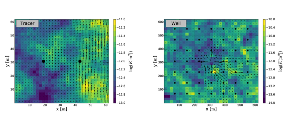
Figure 1: The logarithmic reference permeability fields for the tracer model and the well model with groundwater flow vectors. Measurement locations are depicted as black circles.

The heterogeneous synthetic reference permeability fields, displayed in Figure 1, are generated by sequential MultiGaussian simulation using the software SGSIM (Deutsch and Journel, 1992). The following spherical correlation function is used:

$$\rho(d)=1-\left(\frac{d}{a}\right)\cdot\left[\frac{3}{2}-\frac{1}{2}\cdot\left(\frac{d}{a}\right)\right].$$ (19)

Here, $d$ denotes the Euclidean distance between two grid cells and $a$ is the correlation length of the permeability field. No nugget effect is considered for the generation of the permeability field. Both permeability fields are generated using mean $-12.0\,\log_{10}(K[\mathrm{m}^{2}])$ and standard deviation $0.5\,\log_{10}(K[\mathrm{m}^{2}])$. Correlation lengths of $a=50\,\mathrm{m}$ for the tracer model and $a=60\,\mathrm{m}$ for the well model are used. Note that, relative to the full grid size, the correlation length of the well model is smaller by one order of magnitude.

The ensembles of initial permeability fields for the $1000$ synthetic experiments (for each physical problem set-up, each ensemble size and each EnKF-variant), which we use to compare performance, are generated by SGSim using one set of input parameters, but varying random seeds. A mean logarithmic permeability of $-12.5\,\log_{10}(K[\mathrm{m}^{2}])$ (compared to the reference fields with $-12.0\,\log_{10}(K[\mathrm{m}^{2}])$) and a standard deviation of $0.5\,\log_{10}(K[\mathrm{m}^{2}])$ (identical to the reference fields) are used. Consequently, the EnKF algorithms have to adjust the overall mean of the permeability fields as well as their spatial variability.

3.4 EnKF setup

The EnKF state vector includes permeability, hydraulic head and, for the tracer model, concentration. Permeability is the target parameter of the estimation. Concentration or hydraulic head values serve as the observations which drive the estimation. Measurement noises are assumed constant: $\sigma_{\mathtt{c}}=7.1\times 10^{-3}\mathrm{mol}/\mathrm{l}$ for concentration measurements and $\sigma_{\mathtt{h}}=5\times 10^{-2}\mathrm{m}$ for hydraulic head measurements. These noises resemble the uncertainty of typical measurement devices.

Most EnKF-methods require the specification of additional parameters. The damping factor of Damped EnKF is set to $\alpha=0.1$ (compare (Hendricks Franssen and Kinzelbach, 2008)). In Local EnKF, the length scale $\lambda$ is set to $150\,\mathrm{m}$ for the well model and the tracer model. For Hybrid EnKF, a constant diagonal background covariance matrix is used. The value of $\beta$ used in this study is $0.5$. Results of synthetic experiments, for which $\lambda$ and $\beta$ were varied, can be found in Section 4.5.

In this study a series of EnKF data assimilation experiments, called synthetic experiments, is performed. For each of the methods presented in Section 2.2, seven ensemble sizes (50, 70, 100, 250, 500, 1000 and 2000 realizations) are tested. For the four smaller ensemble sizes, 1000 synthetic experiments are carried out. For the larger ensemble sizes, due to computational limitations, only 100 synthetic experiments are computed.

3.5 Performance evaluation

For a single synthetic experiment with given EnKF-method and ensemble size, the root mean square error is given by

$$\mathrm{RMSE}=\sqrt{\frac{1}{n_{g}}\sum_{l=1}^{n_{g}}\left(\bar{Y}_{l}-Y^{t}_{l}\right)^{2}}.$$ (20)

Here, $n_{g}$ is the number of grid cells, $\bar{\mathbf{Y}}\in R^{n_{g}}$ is the vector containing the estimated mean logarithmic permeabilities across the model domain and $\mathbf{Y}^{t}\in R^{n_{g}}$ is the vector containing the corresponding synthetic reference logarithmic permeabilities.

For each EnKF-method and for a given ensemble size, a large number of synthetic experiments is computed. These synthetic experiments differ solely in the perturbation of initial fields and measurements. A single synthetic experiment provides a sample-RMSE, calculated according to Equation (20) and called $r_{i}^{a,\,n_{e}}$. Taken together, the $n_{syn}=1000$ synthetic experiments (or in the case of large ensembles $n_{syn}=100$ synthetic experiments) for a given method $a$ and ensemble size $n_{e}$ provide an approximate probability density function of the RMSE. We calculate RMSE means according to:

$$\bar{r}^{a,\,n_{e}}=\frac{1}{n_{syn}}\sum_{i=1}^{n_{syn}}r_{i}^{a,\,n_{e}}.$$ (21)

We use these RMSE means to compare EnKF-methods.

The question arises, whether a small number of synthetic experiments $n_{syn}$ would suffice to evaluate the performance of the EnKF-methods. We compare RMSE means of two EnKF-methods on the basis of $n_{syn}=1,\,10,$ or $100$ synthetic experiments. Ten thousand subsets $X$ of $n_{syn}$ synthetic experiments are randomly sampled from the $1000$ synthetic experiments. We calculate and compare the corresponding means $\bar{r}^{a,\,n_{e}}_{X}$. The fraction, for which one EnKF-method $a$ yields a smaller RMSE than another EnKF-method $b$

$$p^{a<b,\,n_{e}}=\frac{\#\{X\mid\bar{r}^{a,\,n_{e}}_{X}<\bar{r}^{b,\,n_{e}}_{X}\}}{10000},$$ (22)

is recorded (the sum $p^{a<b,\,n_{e}}+p^{b<a,\,n_{e}}$ is by definition equal to 1.0). Doing so, we estimate the probability that one method outperforms another method on the basis of $n_{syn}$ synthetic experiments.

Quotients of the RMSE means (based on all 1000 synthetic experiments) for all combinations of EnKF-variants are calculated:

$$q^{a<b,\,n_{e}}=\frac{\bar{r}^{a,\,n_{e}}}{\bar{r}^{b,\,n_{e}}}.$$ (23)

In this formula we choose EnKF-method $a$ to have the smaller RMSE mean, so that $q^{a<b,\,n_{e}}\leq 1$ . From the quotients, we calculate relative differences:

$$d^{a<b,\,n_{e}}=\frac{\bar{r}^{b,\,n_{e}}-\bar{r}^{a,\,n_{e}}}{\bar{r}^{b,\,n_{e}}}=1-q^{a<b,\,n_{e}}.$$ (24)

For example, it could be that EnKF-variant $a$ gives on average (calculated over 1000 synthetic experiments) a RMSE which is $d^{a<b,\,n_{e}}=10\%$ smaller than another EnKF-variant $b$. In that case, the quotient would be $q^{a<b,\,n_{e}}=0.9$. We analyze which relative differences are with at least 95% probability statistically significant for $n_{syn}$ synthetic experiments and which are not.

$$D^{n_{e}}_{+}=\{d^{a<b,\,n_{e}}\mid p^{a<b,\,n_{e}}>0.95\}$$ (25)

$$D^{n_{e}}_{-}=\{d^{a<b,\,n_{e}}\mid p^{a<b,\,n_{e}}\leq 0.95\}$$ (26)

Finally, we compare the smallest significant relative difference

$$d^{min}_{+}=\min D^{n_{e}}_{+}$$ (27)

to the largest insignificant relative difference

$$d^{max}_{-}=\max D^{n_{e}}_{-}.$$ (28)

In general, one would expect $d^{min}_{+}$ to be larger than $d^{max}_{-}$. In this case, we choose the threshold for significant relative differences between the two values. However, due to the specific shape of the RMSE distributions (especially related to their spread), it may occur that $d^{min}_{+}<d^{max}_{-}$. If this happens, we evaluate the comparisons on the basis of their specific distributions and choose the threshold manually.

4 Results and Discussion

4.1 Tracer model

4.1.1 Comparison of EnKF-variants in terms of Mean RMSE

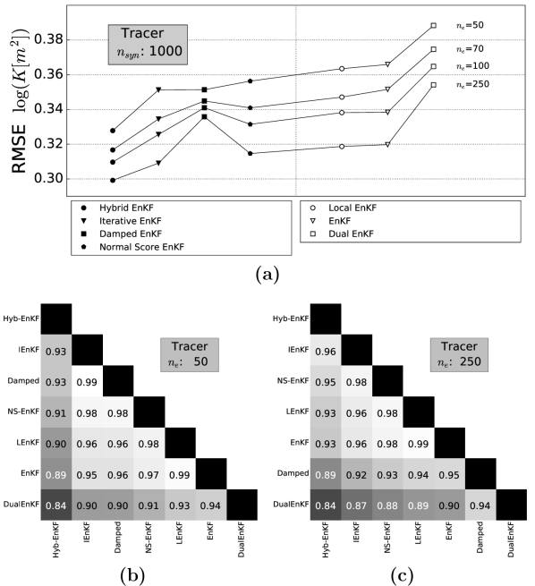
Figure 2: Mean RMSEs for seven EnKF-methods derived from 1000 synthetic experiments for the tracer model - Ensemble Sizes: $n_{e}=50,\,70,\,100,\,250$ (a). For ensemble sizes $n_{e}=50\textrm{ (b)},\,250\textrm{ (c)}$, the RMSE mean for a method on the horizontal axis divided by the RMSE mean for a method on the vertical axis is given.

Figure 2 shows the mean RMSEs for all methods and ensemble sizes 50, 70, 100 and 250. The RMSE values $\bar{r}^{a,\,n_{e}}$ range from $0.3\,\log_{10}(K[\mathrm{m}^{2}])$ to $0.4\,\log_{10}(K[\mathrm{m}^{2}])$. For ensemble size 50, Hybrid EnKF yields the smallest mean RMSE ($0.328\,\log_{10}(K[\mathrm{m}^{2}])$ followed by Iterative EnKF, Damped EnKF and Normal Score EnKF ($0.351\,\log_{10}(K[\mathrm{m}^{2}])$, $0.351\,\log_{10}(K[\mathrm{m}^{2}])$ and $0.356\,\log_{10}(K[\mathrm{m}^{2}])$). Local EnKF ($0.363\,\log_{10}(K[\mathrm{m}^{2}])$) and Classical EnKF ($0.366\,\log_{10}(K[\mathrm{m}^{2}])$) follow. Finally, Dual EnKF yields the largest RMSE: $0.388\,\log_{10}(K[\mathrm{m}^{2}])$.

When the ensemble size is increased from 50 to 250, all methods produce ensemble mean permeability fields closer to the reference. The RMSE for Damped EnKF is $\bar{r}^{\mathrm{Damped},\,50}-\bar{r}^{\mathrm{Damped},\,250}=0.016\,\log_{10}(K[\mathrm{m}^{2}])$ smaller for an ensemble size of 250 than for an ensemble size of 50. This RMSE reduction is the smallest of all EnKF-methods and the next smallest reduction ($\bar{r}^{\mathrm{Hyb-EnKF},\,50}-\bar{r}^{\mathrm{Hyb-EnKF},\,250}=0.029\,\log_{10}(K[\mathrm{m}^{2}])$ smaller for ensemble size 250 than for ensemble size 50) is by Hybrid EnKF. As a result, Damped EnKF has the second largest RMSE among all EnKF-methods for ensemble size 250. The ranking of the remaining methods is identical for all four ensemble sizes.

The second part of Figure 2 contains tables of quotients $q^{a<b,\,50}$ and $q^{a<b,\,250}$ (as defined in Equation (23)) for all pairs of EnKF-methods. The largest relative difference in the tables is $16\%$ (Hybrid EnKF vs Dual EnKF) for both ensemble sizes 50 and 250. Three relative differences are as small as $1\%$ (Iterative EnKF vs Damped EnKF and Local EnKF vs Classical EnKF for ensemble size 50, Local EnKF vs Classical EnKF for ensemble size 250). In the following, we examine which relative differences can be considered significant as function of the number of synthetic experiments.

It is worth mentioning that the mean RMSE difference between initial permeability fields and the synthetic truth ($0.62\,\log_{10}(K[\mathrm{m}^{2}])$) is significantly reduced in all synthetic experiments. Finally, we note that the large RMSEs of Local EnKF, Classical EnKF and Dual EnKF can be attributed at least partially to a non-negligible number of synthetic experiments with very large RMSEs. The full RMSE distributions are shown in Figure 7.

4.1.2 Thresholds on significant RMSE differences

It is evaluated whether significant differences in performance between EnKF-variants can be demonstrated for 1, 10 or 100 synthetic experiments. Figure 3 shows probabilities to find a smaller RMSE mean for a given EnKF-variant compared to another EnKF-variant based on $n_{syn}$ synthetic experiments.

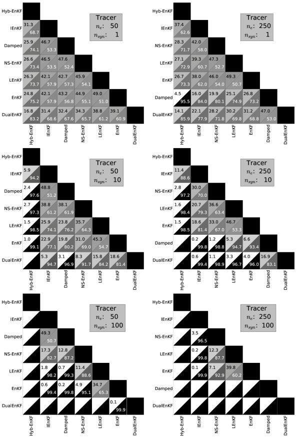
Figure 3: Probabilities to find a smaller RMSE mean for a given EnKF-variant compared to another EnKF-variant, based on 1, 10 and 100 synthetic experiments (tracer model, ensemble sizes 50 and 250).

The probabilities $p^{a<b,\,50}$ and $p^{a<b,\,250}$ from Figure 3 are cross-checked with the quotients $q^{a<b,\,50}$ and $q^{a<b,\,250}$ in Figure 2 to determine thresholds for significant relative RMSE differences. Significant relative differences are defined as the relative differences, for which at least $95\%$ of the comparisons favor one of the two EnKF-methods. Based on a single synthetic experiment, and for ensemble size 50, all relative RMSE differences are insignificant. Consequently, RMSE differences between two EnKF-methods smaller than $16\%$ cannot be detected on the basis of a single synthetic experiment and ensemble size 50. For ensemble size 250, the RMSE difference of $11\%$ for the comparison pair Hybrid EnKF vs Damped EnKF is significant. On the other hand, there are three insignificant comparisons with larger relative differences (Hybrid EnKF vs Dual EnKF, Iterative EnKF vs Dual EnKF and Normal Score EnKF vs Dual EnKF). The anomaly that three insignificant relative differences are larger than a significant relative difference is due to the narrow RMSE distribution of the Damped EnKF (Figure 7 shows that there are fewer RMSEs below $0.3\,\log_{10}(K[\mathrm{m}^{2}])$ for Damped EnKF than for any other method). Taking this into account, we set the threshold for which significant RMSE differences can be detected to $15\%$. For 10 synthetic experiments and ensemble size 50, there are RMSE differences of $7\%$ and $9\%$ that are significant (Hybrid EnKF vs Damped EnKF, Hybrid EnKF vs Normal Score EnKF) and differences of $9\%$ and $10\%$ that are not (Normal Score EnKF vs Dual EnKF, Iterative EnKF vs Dual EnKF). Taking into account the narrow RMSE distribution of the Damped EnKF, the threshold is set to $9\%$. For ensemble size 250, and 10 synthetic experiments, there is a RMSE difference of $5\%$ that is significant (Hybrid EnKF vs Normal Score EnKF) and there are two of $6\%$ that are not (Hybrid EnKF vs Normal Score EnKF, Damped EnKF vs Dual EnKF). The threshold is set to $6\%$. For 100 synthetic experiments and ensemble size 50, there is a difference of $3\%$ that is significant (Normal Score EnKF vs Classical EnKF) and there are three differences of $2\%$ that are not (Iterative EnKF vs Normal Score EnKF, Damped EnKF vs Normal Score EnKF, Normal Score EnKF vs Local EnKF). The threshold is set to $2\%$. For ensemble size 250, there is a difference of $2\%$ that is significant (Iterative EnKF vs Normal Score EnKF) and there are two differences of $2\%$ that are not (Normal Score EnKF vs Local EnKF, Normal Score EnKF vs Classical EnKF). The threshold is set to $2\%$. All thresholds are provided in Table 1.

4.2 Well model

4.2.1 Comparison of EnKF-variants in terms of Mean RMSE

For the well model, EnKF-variants (and ensemble sizes) are compared on the basis of the calculated RMSE means in the same way as for the tracer model. Results for ensemble sizes 50, 70, 100 and 250 are discussed here. Results for ensemble sizes 500, 1000 and 2000 are discussed later in Section 4.3.

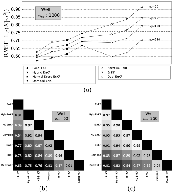
Figure 4: Mean RMSEs for seven EnKF-methods derived from 1000 synthetic experiments for the well model - Ensemble Sizes: $n_{e}=50,\,70,\,100,\,250$ (a). For ensemble sizes $n_{e}=50,\textrm{ (b)},\,250\textrm{ (c)}$, the RMSE mean for a method on the horizontal axis divided by the RMSE mean for a method on the vertical axis is given.

Figure 4 shows the mean RMSEs for all methods and ensemble sizes. The values range from $0.55\,\log_{10}(K[\mathrm{m}^{2}])$ to $0.95\,\log_{10}(K[\mathrm{m}^{2}])$. For the smallest ensemble size of 50, observed mean RMSEs show the largest spread. Local EnKF yields the smallest mean RMSE ($0.63\,\log_{10}(K[\mathrm{m}^{2}])$ followed by Hybrid EnKF, Normal Score EnKF and Damped EnKF ($0.69\,\log_{10}(K[\mathrm{m}^{2}])$, $0.70\,\log_{10}(K[\mathrm{m}^{2}])$ and $0.75\,\log_{10}(K[\mathrm{m}^{2}])$). The methods Iterative EnKF, Classical EnKF and Dual EnKF ($0.81\,\log_{10}(K[\mathrm{m}^{2}])$ and $0.84\,\log_{10}(K[\mathrm{m}^{2}])$, $0.92\,\log_{10}(K[\mathrm{m}^{2}])$) yield mean RMSEs that are larger than those for the initial permeability fields suggesting divergence of the algorithm for a significant fraction of the synthetic experiments.

When the ensemble size is increased from 50 to 250, all methods get closer to the reference. For the methods Local EnKF, Hybrid EnKF, Normal Score EnKF and Damped EnKF the RMSE reduces by up to $0.1\,\log_{10}(K[\mathrm{m}^{2}])$, when the ensemble size is increased from 50 to 250. For Iterative EnKF, Classical EnKF and Dual EnKF this reduction is around $0.2\,\log_{10}(K[\mathrm{m}^{2}])$. As a result, Iterative EnKF ends up with the third smallest RMSE for ensemble size 250, Classical EnKF performs better than Damped EnKF and Dual EnKF still has the largest RMSE, but much closer to the other methods.

The second part of Figure 4 contains tables of quotients $q^{a<b,\,50}$ and $q^{a<b,\,250}$ (as defined in Equation (23)) for all pairs of EnKF-methods. For the well model, the relative differences are much larger than for the tracer model. The largest relative differences in the tables are $32\%$ for ensemble size 50 and $19\%$ for ensemble size 250 (both Local EnKF vs Dual EnKF). For ensemble size 50, the smallest relative difference is $3\%$ for comparison pair Hybrid EnKF vs Normal Score EnKF. For ensemble size 250, two relative differences are at $2\%$ (Hybrid EnKF vs Iterative EnKF, Normal Score EnKF vs Classical EnKF). In general, relative differences are smaller for the larger ensemble size.

The much lower RMSE for ensemble size 250 (compared to ensemble size 50) is most probably related to the overall worse performance of the data assimilation experiments for the well model compared to the tracer model. The worse performance is related to the much smaller correlation length, in combination with the high variance of the permeability field, for this set-up. The benefit of estimating noisy model covariances with a larger ensemble seems therefore to be higher than for the tracer model.

4.2.2 Thresholds on significant RMSE differences

Also for the well model, it is evaluated whether significant differences in performance between EnKF-variants can be demonstrated with 1, 10 or 100 synthetic experiments.

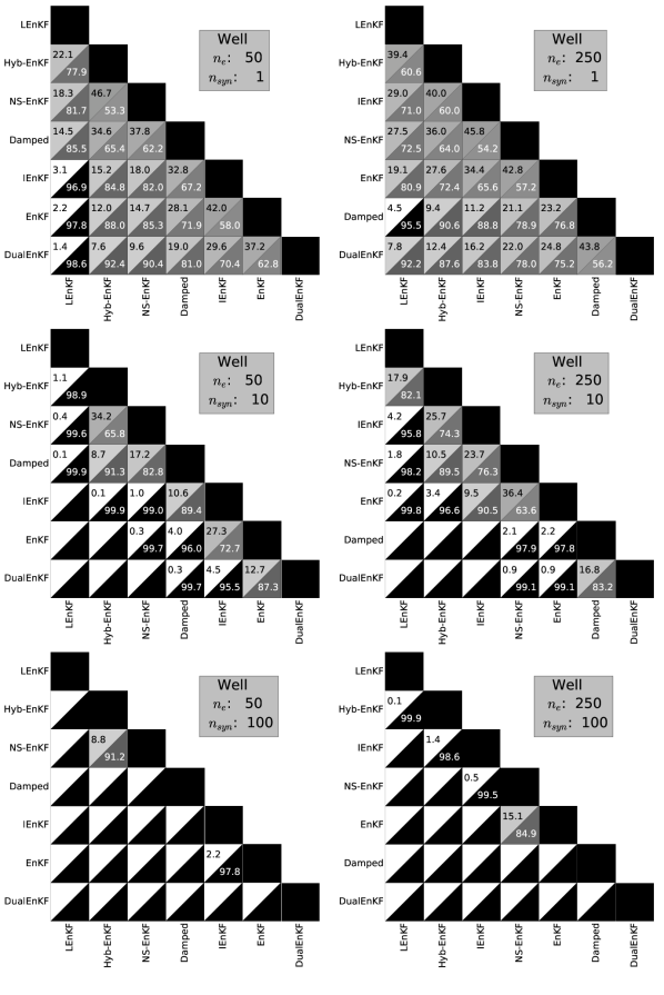
Figure 5: The same as Figure 3 for the well model.

The probabilities $p^{a<b,\,50}$ and $p^{a<b,\,250}$ from Figure 5 are cross-checked with the quotients $q^{a<b,\,50}$ and $q^{a<b,\,250}$ in Figure 4 to determine thresholds for significant relative RMSE differences. For a single synthetic experiment and ensemble size 50, there are significant RMSE differences of $25\%$ and $23\%$ (Local EnKF vs Classical EnKF, Local EnKF vs Iterative EnKF) and insignificant RMSE differences of $24\%$ and $25\%$ (Normal Score EnKF vs Dual EnKF, Hybrid EnKF vs Dual EnKF). The threshold is set to $25\%$. For ensemble size 250, there is the significant case Local EnKF vs Damped EnKF for $15\%$ difference in mean RMSE, but there are also three comparisons with differences $16\%$, $17\%$ and $19\%$ that are not significant (Iterative EnKF vs Dual EnKF, Hybrid EnKF vs Dual EnKF, Local EnKF vs Dual EnKF). As for the tracer set-up, the smallest significant RMSE difference is explained by the relatively narrow distribution of RMSEs for Damped EnKF (compare Figure 7). The threshold is set to $18\%$. For 10 synthetic experiments and ensemble size 50, there are two differences of $9\%$, one is significant (Local EnKF vs Hybrid EnKF) and one is not (Classical EnKF vs Dual EnKF). Thus, the threshold is set to $9\%$. For ensemble size 250, there is a difference of $5\%$ that is significant (Local EnKF vs Iterative EnKF) and there is one of $6\%$ that is not (Damped EnKF vs Dual EnKF). The threshold is set to $5\%$. For 100 synthetic experiments and ensemble size 50, there is a difference of $4\%$ that is significant (Iterative EnKF vs Classical EnKF) and there is one of $3\%$ that is not (Hybrid EnKF vs Normal Score EnKF). The threshold is set to $3\%$. For ensemble size 250, there is a difference of $2\%$ that is significant (Hybrid EnKF vs Iterative EnKF) and there is another one of $2\%$ that is not (Normal Score EnKF vs Classical EnKF). The threshold is set to $2\%$. All thresholds are provided in Table 1.

Table 1: RMSE differences which are considered to be significant for the two simulation set-ups and as a function of the number of synthetic experiments $n_{syn}$ and the number of ensemble members $n_{e}$.

	$n_{syn}$	$n_{e}=50$	$n_{e}=70$	$n_{e}=100$	$n_{e}=250$	$n_{e}=500$	$n_{e}=1000$	$n_{e}=2000$
Tracer	1	$>\,16\%$	$>\,16\%$	$>\,16\%$	15%	13%	15%	14%
	10	9%	9%	8%	6%	6%	5%	4%
	100	2%	3%	3%	2%	-	-	-
Well	1	25%	20%	23%	18%	17%	16%	15%
	10	9%	9%	8%	5%	5%	5%	5%
	100	3%	$<\,3\%$	2%	2%	-	-	-

4.3 Large ensembles

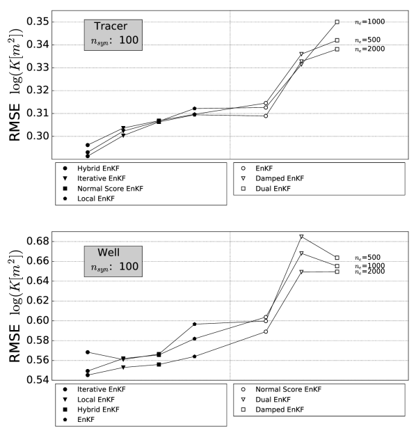
Figure 6: Mean RMSEs for seven EnKF-methods derived from 100 synthetic experiments for the tracer and well model and ensemble sizes 500, 1000 and 2000.

Results from synthetic experiments for ensemble sizes 500, 1000 and 2000 are shown in Figure 6. RMSE means are computed from 100 synthetic experiments instead of the 1000 synthetic experiments which were calculated for the smaller ensemble sizes. This leads to a larger uncertainty in the mean calculation. Additionally, for ensemble sizes 500, 1000 and 2000, RMSE means are very similar. RMSE means are even not always smaller for a larger ensemble size (for example for Dual EnKF and the tracer model, the RMSE mean for ensemble size 500 is smaller than the RMSE mean for ensemble size 1000). The ranking of the performance of the different EnKF-variants for the large ensemble sizes is similar to the method ranking for ensemble size 250. In addition, for larger ensemble sizes the number of synthetic experiments which is needed to show significant difference in performance of EnKF-methods is only marginally smaller than for ensemble size 250 (see Table 1).

4.4 RMSE distributions

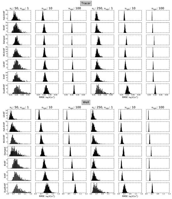
Figure 7: Mean RMSE distributions for ensemble sizes 50 and 250, for 1, 10 and 100 synthetic experiments, for the tracer and well model.

The mean RMSE distributions calculated for the two model set-ups, $n_{syn}=1,10$ or $100$ and ensemble sizes 50 and 250 are displayed in Figure 7. For $n_{syn}=10$ or $100$, the mean RMSE distributions are close to Gaussian, but for $n_{syn}=1$ the spread is larger with more outliers. The narrow distributions calculated on the basis of 100 synthetic experiments, for the different EnKF-methods, show little overlap. Comparing RMSE distributions for ensemble size 50 and 250, it can be seen that there are less outliers for the larger ensemble size. If we compare the RMSE distributions for the tracer and well model, it is clear that especially Damped EnKF has a different distribution from the rest. Whereas it has the narrowest distributions for the tracer set-up, it has one of the widest distributions for the well set-up.

The width of the RMSE distributions illustrates the variability of the estimation results related to the random seed variation. The large overlap of RMSE distributions for the different EnKF-variants suggests that the estimation result is more dependent on the random seed than on the choice of EnKF-method. If we base the analysis on 10 or 100 synthetic experiments, the distributions get narrower allowing to detect significant differences in performance of different EnKF-methods.

4.5 Variation of EnKF-method parameters

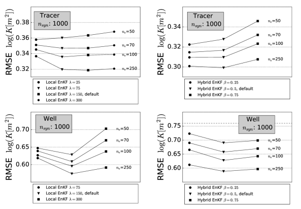
Figure 8: Variation of mean RMSE for Local EnKF and Hybrid EnKF, as a function of values for the parameters $\lambda$ and $\beta$ and ensemble size. Results are shown for both the tracer model and the well model.

For the two methods Local EnKF and Hybrid EnKF, the correlation length $\lambda$ and mixing parameter $\beta$ were varied, respectively. The resulting mean RMSEs are displayed in Figure 8. For the tracer set-up and ensemble size 50, Local EnKF with the smallest correlation length of $25\,\mathrm{m}$ yields the smallest mean RMSE. On the contrary, for larger ensemble sizes the smallest correlation length yields the largest mean RMSE and a correlation length of $150\,\mathrm{m}$ results in the smallest mean RMSE. For the well model, the correlation length of $150\,\mathrm{m}$ yields the smallest mean RMSEs for all ensemble sizes. Although the results are affected by the parameter values, the performance of Local EnKF is not so strongly influenced by the choice of the correlation length in these cases, except for ensemble size 250, for which a small correlation length results in a large RMSE affecting the ranking of the EnKF methods.

For Hybrid EnKF, the parameter $\beta$ also has a certain impact on the performance which is larger for small ensemble sizes. This influences the ranking of the methods, but to a limited extent. These examples also show the importance of parameter settings which add an additional uncertainty component to model comparisons.

4.6 Varying the observation noise

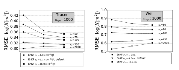
Figure 9: Variation of mean RMSE for different observation noises in Classical EnKF, as function of ensemble size. Results are shown for both the tracer model and the well model.

To illustrate the effect of different observation noises, the tracer and well set-ups were computed for Classical EnKF and observation noises larger and smaller than the noise level chosen for the default synthetic experiment. In Figure 9, the resulting RMSE means are shown for ensemble sizes 50, 70, 100, 250 and 2000. For ensemble size 50, in both set-ups, smaller observation noise leads to larger RMSE means, whereas the larger observation noise leads to smaller RMSE means. This trend changes, when the ensemble size is larger. For ensemble size 2000, in both set-ups, the smallest observation noise results in the smallest RMSE mean.

Results for different observation noises can be understood taking into account two different impacts of observation noise on the simulation results. First, smaller observation noise results in a higher weight for observations, i.e. a stronger correcting influence of the observations. It should result on average in smaller RMSEs as long as its influence is correctly weighted in the filter and it is therefore important that model covariances are correct, which is the case if the ensemble size is large. For small ensemble sizes, model covariances differ more strongly from the true values resulting in an incorrect weighting and the risk that updates go in the wrong direction resulting in larger RMSEs. The default values were originally chosen because they represent the behavior of typical measurement devices. According to these results, they also seem to constitute a sensible trade-off between filter divergence due to unjustifiably small observation noise and information loss due to unjustifiably large observation noise.

4.7 Discussion

The tracer model and the well model have different boundary conditions, different correlation lengths of the reference permeability fields and different measurement types and amounts which are assimilated. The data assimilation experiments for each of these two model set-ups result in different RMSE values. Nevertheless, for the two model set-ups similar conclusions are reached in terms of the number of synthetic experiments which is needed to show that one EnKF-variant outperforms another one. Given these results, we recommend that for comparisons of EnKF-variants 10 or more synthetic experiments are needed. A number of 10 synthetic experiments is needed to show that one EnKF-variant significantly outperforms another EnKF-variant if the two methods show a difference in RMSE of at least 10%. It can be argued that a RMSE difference of 10% is important enough to be detected. For really small RMSE differences of 2% around 100 synthetic experiments are needed.

The study only considers variations in the initial ensemble of rock permeabilities. However, in reality we face other sources of uncertainty like additional uncertain parameters, model forcings and boundary conditions, which affect the study outcome. Therefore we feel that the main conclusion of this paper, the need for ten or more synthetic experiments to compare different EnKF-variants, is not overly pessimistic, taking into account that several other factors also determine the relative performance of methods.

If we focus on the ranking of the EnKF-methods, we find that the physical model set-up and measurement type have a strong influence on the ranking of the EnKF-methods. The synthetic experiments featuring 2 tracer measurements lead to permeability fields that were closer to the corresponding synthetic true than the synthetic experiments featuring 48 head measurements. The magnitude of the observation noise, which should in principle be determined by the measurements, was also observed to influence filter performance. The degree of heterogeneity of the permeability field might also influence the relative performance of a given EnKF-variant. For example, Iterative EnKF might perform relatively better (compared to other EnKF-variants) for strongly heterogeneous permeability fields as non-linearity is more an issue for those fields. On the other hand, for strongly non-Gaussian permeability fields it is expected that Normal Score EnKF will improve its relative performance compared to other methods. For Local EnKF and Hybrid EnKF, an influence of the parameter choice on the filter performance was observed.

The ranking of the methods also differed between the two physical model set-ups, emphasizing even more that the comparison of EnKF-variants is not straightforward and not only affected by random fluctuations related to the synthetic case, but also to other factors. We want to stress that therefore we do not attempt to rank the EnKF-variants, but want to show the impact of random factors and also the physical model set-up on the comparison of EnKF-variants.

5 Conclusion

Seven EnKF-variants (Damped EnKF, Iterative EnKF, Local EnKF, Hybrid EnKF, Dual EnKF, Normal Score EnKF, Classical EnKF) have been applied for joint state-parameter estimation for the two model set-ups, a 2D groundwater flow - tracer transport model and a 2D groundwater flow model with an injection well. For each model, each EnKF-variant and seven different ensemble sizes (50, 70, 100, 250, 500, 1000, 2000), 1000 synthetic experiments (100 for the three larger ensemble sizes) were calculated. These synthetic experiments used different initial sets of permeability fields. RMSE values, which measure the distance between estimated and reference permeabilities, were calculated. On the basis of the many repetitions of synthetic experiments, a RMSE pdf could be constructed for each EnKF-variant and ensemble size. RMSE means of these distributions were used to compare EnKF-variants. Additionally, differences in performance between two methods were compared for means calculated from 1, 10 or 100 synthetic experiments.

Thresholds on relative RMSE differences that can be significantly detected using 1, 10 or 100 synthetic experiments are given. Single synthetic experiments are generally not enough to show a significant difference in performance of EnKF-variants, even when these EnKF-variants result in RMSE differences of $15\%$. In this study, 10 synthetic experiments were not enough to show that relative RMSE differences between EnKF-variants smaller than 10% are significant. In our models, 100 synthetic experiments allow to show that RMSE differences between EnKF-variants larger than 2% are significant. As in addition other sources of uncertainty play a role in real-world studies and could be considered as well in comparison studies, we feel that at least 10 synthetic experiments are needed to rigorously compare two EnKF-variants.

6 Acknowledgments

This study was supported by the Deutsche Forschungsgemeinschaft. Simulations were performed with computing resources granted by RWTH Aachen University under project rwth0009. The data used are available through a data repository (https://doi.org/10.5281/zenodo.1343571). Under https://doi.org/10.5281/zenodo.1344337 corresponding Python scripts are archived.

References

- (1)
- Anderson (2001) Anderson, J. L. (2001), An Ensemble Adjustment Kalman Filter for Data Assimilation, Mon. Weather Rev., 129(12), 1884–2903, 10.1175/1520-0493(2001)129<2884:aeakff>2.0.co;2.
- Baatz et al. (2017) Baatz, D., Kurtz, W., Hendricks Franssen, H. J., Vereecken, H., and Kollet, S. J. (2017), Catchment tomography - An approach for spatial parameter estimation, Adv. Water Resour., 107, 147–159, 10.1016/j.advwatres.2017.06.006.
- Bear (1972) Bear, J. (1972), Dynamics of Fluids in Porous Media, American Elsevier Pub. Co.
- Burgers et al. (1998) Burgers, G., van Leeuwen, P. J., and Evensen, G. (1998), Analysis Scheme in the Ensemble Kalman Filter, Mon. Weather Rev., 126(6), 1719–1724, 10.1175/1520-0493(1998)126<1719:asitek>2.0.co;2.
- Camporese et al. (2009) Camporese, M., Paniconi, C., Putti, M., and Salandin, P. (2009), Comparison of Data Assimilation Techniques for a Coupled Model of Surface and Subsurface Flow, Vadose Zone J., 8(4), 1539–1663, 10.2136/vzj2009.0018.
- Carrera and Neuman (1986) Carrera, J., and Neuman, S. P. (1986), Estimation of Aquifer Parameters Under Transient and Steady State Conditions: 1. Maximum Likelihood Method Incorporating Prior Information, Water Resour. Res., 22(2), 199–210, 10.1029/wr022i002p00199.
- Chen (2003) Chen, Z. (2003), Bayesian Filtering: From Kalman Filters to Particle Filters, and Beyond, Statistics, 182(1), 1–69.
- Chen and Zhang (2006) Chen, Y., and Zhang, D. (2006), Data assimilation for transient flow in geologic formations via ensemble Kalman filter, Adv. Water Resour., 29(8), 1107–1122, 10.1016/j.advwatres.2005.09.007.
- Chen and Oliver (2010) Chen, Y., and Oliver, D. S. (2010), Cross-covariances and localization for EnKF in multiphase flow data assimilation, Comput. Geosci., 14(4), 579–601, 10.1007/s10596-009-9174-6.
- Clauser (2012) Clauser, C. (2012), Numerical Simulation of Reactive Flow in hot Aquifers: SHEMAT and Processing SHEMAT, Springer Science & Business Media.
- De Lannoy and Reichle (2016) De Lannoy, G. J. M., and Reichle, R. H. (2016), Assimilation of SMOS brightness temperatures or soil moisture retrievals into a land surface model, Hydrol. Earth Syst. Sc., 20(12), 4895–4911, 10.5194/hess-20-4895-2016.
- Deutsch and Journel (1992) Deutsch, C. V., and Journel, A. G. (1992), Geostatistical software library and user’s guide, New York, 119, 147.
- Devegowda et al. (2010) Devegowda, D., Arroyo-Negrete, E., and Datta-Gupta, A. (2010), Flow relevant covariance localization during dynamic data assimilation using EnKF, Adv. Water Resour., 33(2), 129–145, 10.1016/j.advwatres.2009.10.001.
- Emerick and Reynolds (2011) Emerick, A. A., and Reynolds, A. C. (2011), Combining sensitivities and prior information for covariance localization in the ensemble Kalman filter for petroleum reservoir applications, Comput. Geosci., 15(2), 251–269, 10.1007/s10596-010-9198-y.
- Evensen (1994) Evensen, G. (1994), Sequential data assimilation with a nonlinear quasi-geostrophic model using Monte Carlo methods to forecast error statistics, J. Geophys. Res-Oceans, 99(C5),10143–10162, 10.1029/94jc00572.
- Evensen (2003) Evensen, G. (2003), The Ensemble Kalman Filter: theoretical formulation and practical implementation, Ocean Dynam., 53(4), 343–367, 10.1007/s10236-003-0036-9.
- Gaspari and Cohn (1999) Gaspari, G., and Cohn, S. E. (1999), Construction of Correlation Functions in Two and Three Dimensions, Q. J. Roy. Meteor. Soc., 125(554),723–757, 10.1002/qj.49712555417.
- El Gharamti et al. (2013) El Gharamti, M., Hoteit, I., and Valstar, J. (2013), Dual states estimation of a subsurface flow-transport coupled model using ensemble Kalman filtering, Adv. Water Resour., 60, 75–88, 10.1016/j.advwatres.2013.07.011.
- El Gharamti and Hoteit (2014) El Gharamti M., and Hoteit, I. (2014), Complex step-based low-rank extended Kalman filtering for state-parameter estimation in subsurface transport models, J. Hydrol., 509, 588–600, 10.1016/j.jhydrol.2013.12.004.
- El Gharamti et al. (2014) El Gharamti, M., Valstar, J., and Hoteit, I. (2014), An adaptive hybrid EnKF-OI scheme for efficient state-parameter estimation of reactive contaminant transport models, Adv. Water Resour., 71, 1–15, 10.1016/j.advwatres.2014.05.001.
- El Gharamti et al. (2015) El Gharamti, M., Ait-El-Fquih, B., and Hoteit, I. (2015), An iterative ensemble Kalman filter with one-step-ahead smoothing for state-parameters estimation of contaminant transport models, J. Hydrol., 527, 442–457, 10.1016/j.jhydrol.2015.05.004.
- Gómez-Hernánez et al. (1997) Gómez-Hernánez, J. J., Sahuquillo, A., and Capilla, J. (1997), Stochastic simulation of transmissivity fields conditional to both transmissivity and piezometric data—I. Theory, J. Hydrol., 203(1), 162–174, 10.1016/s0022-1694(97)00098-x.
- Goovaerts (1997) Goovaerts, P. (1997), Geostatistics for natural resources evaluation, Oxford University Press on Demand.
- Hamill and Snyder (2000) Hamill, T. M., and Snyder, C. (2000), A Hybrid Ensemble Kalman Filter-3D Variational Analysis Scheme, Mon. Weather Rev., 128(8), 2905–2919, 10.1175/1520-0493(2000)128<2905:ahekfv>2.0.co;2.
- Hamill et al. (2001) Hamill, T. M., Whitaker, J. S., and Snyder, C. (2001), Distance-Dependent Filtering of Background Error Covariance Estimates in an Ensemble Kalman Filter, Monthly Weather Review, 129(11), 2776–2790, 10.1175/1520-0493(2001)129<2776:ddfobe>2.0.co;2.
- Hendricks Franssen et al. (2003) Hendricks Franssen, H. J., Gómez-Hernández, J., and Sahuquillo, A. (2003), Coupled inverse modelling of groundwater flow and mass transport and the worth of concentration data, J. Hydrol., 281(4), 281–295, 10.1016/s0022-1694(03)00191-4.
- Hendricks Franssen and Kinzelbach (2008) Hendricks Franssen, H. J., and Kinzelbach, W. (2008), Real-time groundwater flow modeling with the Ensemble Kalman Filter: Joint estimation of states and parameters and the filter inbreeding problem, Water Resour. Res., 44(9), 1–21, 10.1029/2007wr006505.
- Hendricks Franssen and Kinzelbach (2009) Hendricks Franssen, H. J., and Kinzelbach, W. (2009), Ensemble Kalman filtering versus sequential self-calibration for inverse modelling of dynamic groundwater flow systems, J. Hydrol., 365(3-4), 261–274, 10.1016/j.jhydrol.2008.11.033.
- Houtekamer and Mitchell (1998) Houtekamer, P. L. and Mitchell, H. L. (1998), Data Assimilation Using an Ensemble Kalman Filter Technique, Mon. Weather Rev., 126(3), 796–811, 10.1175/1520-0493(1998)126<0796:dauaek>2.0.co;2.
- Huyakorn (2012) Huyakorn, P. S. (2012), Computational methods in subsurface flow, Academic Press.
- Journel and Huijbregts (1978) Journel, A. G., and Huijbregts, C. J. (1978), Mining geostatistics, Academic press.
- Kalman et al. (1960) Kalman, R. E. et al. (1960), A New Approach to Linear Filtering and Prediction Problems, J. Basic Eng., 82(1), 35–45, 10.1115/1.3662552.
- Kalnay (2002) Kalnay, E. (2002), Atmospheric modeling, data assimilation and predictability, Cambridge Univ. Press, New York.
- Kitanidis and Vomvoris (1983) Kitanidis, P. K., and Vomvoris, E. G. (1983), A Geostatistical Approach to the Inverse Problem In Groundwater Modeling (Steady State) and One-Dimensional Simulations, Water Resour. Res., 19(3), 677–690, 10.1029/wr019i003p00677.
- Kurtz et al. (2014) Kurtz, W., Hendricks Franssen, H. J., Kaiser, H. P., and Vereecken, H. (2014), Joint assimilation of piezometric heads and groundwater temperatures for improved modeling of river-aquifer interactions, Water Resour. Res., 50(2), 1665–1688, 10.1002/2013wr014823.
- Li et al. (2012) Li, L., Zhou, H., Hendricks Franssen, H. J., Gómez-Hernández, J. J. (2012), Groundwater flow inverse modeling in non-MultiGaussian media: performance assessment of the normal-score Ensemble Kalman Filter, Hydrol. Earth Syst. Sc., 16(2), 573–590, 10.5194/hess-16-573-2012.
- Liu et al. (2016) Liu, B., Gharamti, M. E., and Hoteit, I. (2016), Assessing clustering strategies for Gaussian mixture filtering a subsurface contaminant model, J. Hydrol., 535, 1–21, 10.1016/j.jhydrol.2016.01.048.
- Lynch (2005) Lynch, D. R. (2005), Numerical Partial Differential Equations for Environmental Scientists and Engineers: A Practical First Course, Springer Science & Business Media.
- Lorentzen et al. (2003) Lorentzen, R. J., Nævdal, G., and Lage, A. (2003), Tuning of parameters in a two-phase flow model using an ensemble Kalman Filter, Int. J. Multiphas. Flow, 29(8), 1283-1309, 10.1016/s0301-9322(03)00088-0.
- Moradkhani et al. (2005) Moradkhani, H., Sorooshian, S., Gupta, H. V., and Houser, P. R. (2005), Dual state–parameter estimation of hydrological models using ensemble Kalman filter, Adv. Water Resour., 28(2), 135–147, 10.1016/j.advwatres.2004.09.002.
- Naevdal et al. (2005) Naevdal, G., Johnsen, L. M., Aanonsen, S. I., and Vefring, E. H., Reservoir Monitoring and Continuous Model Updating Using Ensemble Kalman Filter, Soc. Petrol. Eng. J., 10(1), 66-74, 10.2118/84372-pa.
- Nowak (2009) Nowak, W. (2009), Best unbiased ensemble linearization and the quasi-linear Kalman ensemble generator, Water Resour. Res., 45(4), 1–17, 10.1029/2008wr007328.
- RamaRao et al. (1995) RamaRao, B. S., LaVenue, A. M., De Marsily, G., and Marietta, M. G. (1995), Pilot point methodology for automated calibration of an ensemble of conditionally simulated transmissivity fields: 1. Theory and computational experiments, Water Resour. Res., 13(3), 475–493, 10.1029/94wr02258.
- Rath et al. (2006) Rath, V., Wolf, A., and Bücker, H. (2006), Joint three-dimensional inversion of coupled groundwater flow and heat transfer based on automatic differentiation: sensitivity calculation, verification, and synthetic examples, Geophys. J. Int., 167(1), 453–466, 10.1111/j.1365-246x.2006.03074.x.
- Reichle et al. (2002) Reichle, R. H., McLaughlin, D. B., and Entekhabi, D. (2002), Hydrologic Data Assimilation with the Ensemble Kalman Filter, Mon. Weather Rev., 130(1), 103–114, 10.1175/1520-0493(2002)130<0103:hdawte>2.0.co;2.
- Sakov et al. (2012) Sakov, P., Oliver, D. S., and Bertino, L. (2012), An Iterative EnKF for Strongly Nonlinear Systems, Mon. Weather Rev., 140(6), 1988–2004, 10.1175/mwr-d-11-00176.1.
- Schöniger et al. (2012) Schöniger, A., Nowak, W., and Hendricks Franssen, H. J. (2012), Parameter estimation by ensemble Kalman filters with transformed data: Approach and application to hydraulic tomography, Water Resour. Res., 48(4), 10.1029/2011wr010462.
- Shi et al. (2014) Shi, Y., Davis, K. J., Zhang, F., Duffy, C. J., and Yu, X. (2014), Parameter estimation of a physically based land surface hydrologic model using the ensemble Kalman filter: A synthetic experiment, Water Resour. Res., 50(1), 706–724, 10.1002/2013wr014070.
- Sun et al. (2009a) Sun, A. Y., Morris, A. P., and Mohanty, S. (2009a), Comparison of deterministic ensemble Kalman filters for assimilating hydrogeological data, Adv. Water Resour., 32(2), 280–292, 10.1016/j.advwatres.2008.11.006.
- Sun et al. (2009b) Sun, A. Y., Morris, A. P., and Mohanty, S. (2009b), Sequential updating of multimodal hydrogeologic parameter fields using localization and clustering techniques, Water Resour. Res., 45(7), 10.1029/2008wr007443.
- Van der Vorst (1992) Van der Vorst, H. A. (1992), Bi-CGSTAB: A Fast and Smoothly Converging Variant of Bi-CG for the Solution of Nonsymmetric Linear Systems, SIAM J. Sci. Stat. Comp., 13(2), 631–644, 10.1137/0913035.
- Vogt et al. (2012) Vogt, C., Marquart, G., Kosack, C., Wolf, A., and Clauser, C. (2012), Estimating the permeability distribution and its uncertainty at the EGS demonstration reservoir Soultz-sous-Forêts using the ensemble Kalman filter, Water Resour. Res., 48(8), 1–15, 10.1029/2011wr011673.
- Vrugt et al. (2005) Vrugt, J. A., Diks, C. G. H., Gupta, H. V., Bouten, W., and Verstraten, J. M. (2005), Improved treatment of uncertainty in hydrologic modeling: Combining the strengths of global optimization and data assimilation, Water Resour. Res., 41(1), 1–17, 10.1029/2004wr003059.
- Wan and Nelson (2001) Wan, E. A., and Nelson, A. T. (2001), Dual Extended Kalman Filter Methods, Kalman filtering and neural networks, 123–173, 10.1002/0471221546.ch5.
- Wu and Margulis (2011) Wu, C. C., and Margulis, S. A. (2011), Feasibility of real-time soil state and flux characterization for wastewater reuse using an embedded sensor network data assimilation approach, J. Hydrol., 399(3), 313–325, 10.1016/j.jhydrol.2011.01.011.
- Zhou et al. (2011) Zhou, H., Gómez-Hernández, J. J., Hendricks Franssen, H.-J., and Li, L. (2011), An approach to handling non-Gaussianity of parameters and state variables in ensemble Kalman filtering, Adv. Water Resour., 34(7), 844–864, 10.1016/j.advwatres.2011.04.014.