Collective mode reductions for populations of coupled noisy oscillators

Abstract

We analyze accuracy of different low-dimensional reductions of the collective dynamics in large populations of coupled phase oscillators with intrinsic noise. Three approximations are considered: (i) the Ott-Antonsen ansatz, (ii) the Gaussian ansatz, and (iii) a two-cumulant truncation of the circular cumulant representation of the original system’s dynamics. For the latter we suggest a closure, which makes the truncation, for small noise, a rigorous first-order correction to the Ott-Antonsen ansatz, and simultaneously is a generalization of the Gaussian ansatz. The Kuramoto model with intrinsic noise, and the population of identical noisy active rotators in excitable states with the Kuramoto-type coupling, are considered as examples to test validity of these approximations. For all considered cases, the Gaussian ansatz is found to be more accurate than the Ott-Antonsen one for high-synchrony states only. The two-cumulant approximation is always superior to both other approximations.

Synchrony of large ensembles of coupled elements can be characterised by the order parameters – the mean fields. Quite often the evolution of these collective variables is surprisingly simple, what makes a description with only a few order parameters feasible. Thus, one tries to construct accurate closed low-dimensional mathematical models for the dynamics of the first few order parameters. These models represent useful tools for gaining insight into the underlaying mechanisms of some more sophisticated collective phenomena: for example, one describes coupled populations by virtue of coupled equations for the relevant order parameters. A regular approach to the construction of closed low-dimensional systems is also beneficial for dealing with phenomena, which are beyond the applicability scope of these models; for instance, with such an approach, one can determine constrains on clustering in populations. There are two prominent types of situations, where the low-dimensional models can be constructed: (i) for a certain class of ideal paradigmatic systems of coupled phase oscillators, the Ott-Antonsen ansatz yields an exact equation for the main order parameter; (ii) the Gaussian approximation for the probability density of the phases, also yielding a low-dimensional closure, is frequently quite accurate. In this paper, we compare applications of these two model reductions for situations, where neither of them is perfectly accurate. Furthermore, we construct a new reduction approach which practically works as a first-order correction to the best of the two basic approximations.

I Introduction

Models of globally coupled oscillators are relevant for many applications in physics, engineering, living and social systems Pikovsky-Rosenblum-Kurths-2001-2003 ; Strogatz-2003 ; Filatrella-Nielsen-Pedersen-2008 ; Winfree-2001 ; Acebron-etal-2005 ; Pikovsky-Rosenblum-15 . The main effect here is synchronization, i.e. appearance of a nontrivial mean field due to interactions. This effect can be viewed as a nonequilibrium phase transtion, where the appearing ordered synchronized state is described by a set of order parameters. The famous Kuramoto model of coupled phase oscillators is a paradigmatic example for the synchronization transition, it is completely solvable in the thermodynamic limit of an infinite population. The properties of the transition are also quite well understood if additionally to the coupling, the oscillators are subject to independent noise terms.

A description of globally coupled noisy oscillators can be reduced, in the thermodynamic limit of large ensemble, to a nonlinear Fokker-Planck equation (or to a Liouville equation in the noiseless case), which is a system with an infinite number of degrees of freedom. If one wants not simply find the stationary solutions, but to follow the evolution of the distributions, the problem of the reduction of the infinite-dimensional system to several essential degrees of freedom arises. This closure problem is in the focus of this paper. We will discuss and compare three variants of the reduction to a few global modes: (i) the Ott-Antonsen ansatz Ott-Antonsen-2008 , (ii) the Gaussian ansatz, recently considered by Hannay et al. Hannay-Forger-Booth-2018 on the basis of previous works Zaks-etal-2003 ; Sonnenschein-Schimansky-Geier-2013 ; Sonnenschein-etal-2015 , and (iii) the circular cumulant approach suggested in Ref. Tyulkina-etal-2018 . Neither of these approaches is exact for a population of coupled noisy oscillators, but they provide quite good approximations of the observed regimes. We will compare their accuracy for different ranges of parameters.

II Basic Models

Our basic model is a population of phase oscillators $\varphi_{k}(t)$ with intrinsic noise:

$$\dot{\varphi}_{k}=\omega_{k}+\mathrm{Im}(2h(t)e^{-i\varphi_{k}})+\sqrt{D}\eta_{k}(t)\,.$$ (1)

Here natural frequencies $\omega_{k}$ have a Lorentzian (Cauchy) distribution $g(\omega)=\gamma/[\pi((\omega-\omega_{0})^{2}+\gamma^{2})]$, and $\gamma$ is the distribution half-width. Parameter $D$ is the noise intensity, terms $\eta_{k}$ are independent normalized white Gaussian random forces: $\langle\eta_{k}(t)\eta_{m}(t^{\prime})\rangle=2\delta_{km}\delta(t-t^{\prime})$, $\langle\eta_{k}\rangle=0$. The coupling is determined by the complex force $h$, common for all oscillators. For the Kuramoto setup, this force is proportional to the mean field which is just the Kuramoto order parameter of the population

$$h=\frac{K}{2}Z_{1},\qquad Z_{1}=\langle e^{i\varphi}\rangle=\frac{1}{N}\sum_{j=1}^{N}e^{i\varphi_{j}}\;.$$

The Kuramoto model for noisy oscillators thus reads

$$\dot{\varphi}_{k}=\omega_{k}+\frac{K}{N}\sum_{j=1}^{N}\sin(\varphi_{j}-\varphi_{k})+\sqrt{D}\eta_{k}(t)\,.$$ (2)

With a slight modification of the common force $h$, namely

$$h=\frac{a}{2}+\frac{K}{2}Z_{1}\,,$$

one obtains the equations for a population of noisy active rotators with the Kuramoto-type coupling, treated in Ref. Zaks-etal-2003 :

$$\dot{\varphi}_{k}=\omega_{k}-a\sin\varphi_{k}+\frac{K}{N}\sum_{j=1}^{N}\sin(\varphi_{j}-\varphi_{k})+\sqrt{D}\eta_{k}(t)\,.$$ (3)

Models (2) and (3) are the basic systems we consider below.

III Mode equations

In the thermodynamic limit $N\to\infty$, starting from the Langevin equations (1), one can write for the distribution density of the subpopulation of the oscillators with natural frequency $\omega$ the Fokker-Planck equation

$$\frac{\partial w(\varphi,t|\omega)}{\partial t}=-\frac{\partial}{\partial\varphi}\left[\mathrm{Im}(2h(t)e^{-i\varphi})w\right]+D\frac{\partial^{2}}{\partial\varphi^{2}}w\,.$$ (4)

This equation can be rewritten as an infinite system for the complex amplitudes of the Fourier modes

$$z_{m}=\int_{-\pi}^{\pi}\mathrm{d}\varphi\,w(\varphi,t|\omega)e^{im\varphi}$$

of the density $w(\varphi,t|\omega)=(2\pi)^{-1}\sum_{m}z_{m}(t,\omega)e^{-im\varphi}$:

$$\dot{z}_{n}=ni\omega z_{n}+nhz_{n-1}-nh^{\ast}z_{n+1}-n^{2}Dz_{n}\,.$$ (5)

The quantities $z_{n}$ are the local order parameters at a given frequency, the global Kuramoto-Daido order parameters are obtained by the additional averaging over the distribution of the natural frequencies:

$$Z_{n}=\int\mathrm{d}\omega\,g(\omega)z_{n}\,.$$ (6)

The main order parameter $Z_{1}$ is employed in the definition of the forces $h$ in the two models we study in this paper. Below we consider only the Lorentzian distribution $g$ and adopt the assumption by Ott and Antonsen Ott-Antonsen-2008 on the analyticity of $z_{n}(t,\omega)$ as a function of complex $\omega$ in the upper half-plane. This allows for calculating the global Kuramoto-Daido order parameters via residues as

$$Z_{n}=z_{n}(\omega_{0}+i\gamma)\,.$$

In this way, one obtains an infinite system of equations for $Z_{n}$ (which are in fact moments $\left\langle\left(e^{i\varphi}\right)^{n}\right\rangle$ of the complex observable $e^{i\varphi}$) with $Z_{0}\equiv 1$:

$$\dot{Z}_{n}=n(i\omega_{0}-\gamma)Z_{n}+nhZ_{n-1}-nh^{\ast}Z_{n+1}-n^{2}DZ_{n}\,.$$ (7)

IV Finite-dimensional reductions

As we discussed above, it is desirable to reduce, at least approximately, the infinite system (7) to a finite-dimensional one, and, in what follows, we discuss three ways to accomplish this.

IV.1 Ott-Antonsen reduction

Here one assumes, following Ref. Ott-Antonsen-2008 , that all the higher order parameters can be expressed via the first one according to

$$Z_{n}=(Z_{1})^{n}.$$ (8)

This reduces the system (7) to just one equation

$$\dot{Z}_{1}=(i\omega_{0}-\gamma)Z_{1}+h-h^{\ast}Z_{1}^{2}-DZ_{1}\,.$$ (9)

The Ott-Antonsen (OA) reduction works exactly for $D=0$, where it defines the so-called OA invariant manifold. This manifold corresponds to the probability density being the wrapped Cauchy distribution of the phases.

IV.2 Gaussian reduction

Recently, on the basis of the analysis of some experimental data, another representation of the higher order parameters through the first one was suggested Hannay-Forger-Booth-2018 :

$$Z_{m}=|Z_{1}|^{m^{2}-m}Z_{1}^{m}\,.$$ (10)

Equivalently, if we introduce the amplitude and the argument of the Kuramoto order parameter $Z_{1}=R_{1}e^{i\psi}$, with $R_{1}=\exp[-s^{2}/2]$, we can rewrite (10) as

$$Z_{m}=R_{1}^{m^{2}}e^{im\psi}=e^{-\frac{1}{2}m^{2}s^{2}}e^{im\psi}.$$ (11)

This relation means that the corresponding probability density of the phases is the wrapped Gaussian distribution. Substitution of (10) into Eq. (7) for $n=1$ yields Hannay-Forger-Booth-2018

$$\dot{Z}_{1}=(i\omega_{0}-\gamma)Z_{1}+h-h^{\ast}|Z_{1}|^{2}Z_{1}^{2}-DZ_{1}\,.$$ (12)

IV.3 Cumulant reduction

Recently, we suggested Tyulkina-etal-2018 a reformulation of the model in terms of the “circular cumulants” $\varkappa_{n}$, instead of the formulation in terms of moments (7). The cumulants are determined via the power series of the cumulant-generating function defined as

$$\Psi(k)=k\frac{\partial}{\partial k}\langle\exp(ke^{i\varphi})\rangle\equiv\sum_{n=1}^{\infty}\varkappa_{n}k^{n}\,.$$ (13)

For example, the first three circular cumulants are: $\varkappa_{1}=Z_{1}$, $\varkappa_{2}=Z_{2}-Z_{1}^{2}$, and $\varkappa_{3}=(Z_{3}-3Z_{2}Z_{1}+2Z_{1}^{3})/2$.

The merit of the reformulation in terms of the cumulants is two-fold.
(i) In terms of the cumulants, the OA manifold (8) is a state with one non-vanishing cumulant only: $\varkappa_{1}=Z_{1}$ and $\varkappa_{n>1}=0$. This allows for a representation of the states close to the OA solution as those with small higher cumulants. The cumulants $\varkappa_{2},\varkappa_{3},\ldots$ describe deviations from the OA manifold (from the wrapped Cauchy distribution), see below Fig. 1 for a visualization of the perturbation due to $\varkappa_{2}$.
(ii) For general states with high synchrony, where $|Z_{1}|\approx 1$, the moments $Z_{n}$ decay slowly with $n$, while in terms of cumulants one has $|\varkappa_{1}|\approx 1$ and $|\varkappa_{n>1}|\ll 1$, which also allows for a nice representation in terms of cumulants. In particular, in the case of the wrapped Gaussian distribution (11), the cumulants obey the hierarchy of smallness for arbitrary degree of synchrony; this hierarchy has a simple analytical form for high and low synchrony:

$$\varkappa_{n}=\begin{cases}\frac{-(-n)^{n-2}}{(n-1)!}e^{in\psi}s^{2(n-1)}\left(1+\mathcal{O}(s^{2})\right)&\textrm{for }s^{2}\ll 1\,,\\ (-1)^{n-1}Z_{1}^{n}\left(1+\mathcal{O}(Z_{1}^{2})\right)&\textrm{for }s^{2}\gtrsim 1\,.\end{cases}$$ (14)

Hence, the cumulant representation appears to be a proper framework for perturbations both of the OA solution and of a highly synchronous state, although the exact equation system for the cumulants Tyulkina-etal-2018 is more complex than (7):

$$\begin{array}[]{l}\dot{\varkappa}_{n}=n(i\omega_{0}-\gamma)\varkappa_{n}+h\delta_{1n}\\ \qquad-h^{\ast}(n^{2}{\varkappa}_{n+1}+n\sum\limits_{m=0}^{n-1}\varkappa_{n-m}\varkappa_{m+1})\\ \qquad\qquad-D(n^{2}{\varkappa}_{n}+n\sum\limits_{m=0}^{n-2}\varkappa_{n-1-m}\varkappa_{m+1})\,.\end{array}$$ (15)

Note, that Eqs. (7) and (15) describe nonidentical oscillators with Lorentzian distribution of frequencies; identical ensembles correspond to $\gamma=0$.

In Ref. Tyulkina-etal-2018 , the infinite system (15) was analysed in the case of small noise intensity $D$, and was shown to generate, as a perturbation of the OA solution, the hierarchy $\varkappa_{n}\sim D^{n-1}$ for $n\geq 2$. A first-order correction to the OA ansatz requires the cumulant $\varkappa_{2}$ to be taken into account; from the infinite system (15) only two equations remain:

$$\begin{array}[]{l}\dot{Z}_{1}=(i\omega_{0}-\gamma)Z_{1}+h-h^{\ast}(Z_{1}^{2}+\varkappa_{2})-DZ_{1}\,,\\[5.0pt] \dot{\varkappa}_{2}=2(i\omega_{0}-\gamma)\varkappa_{2}-4h^{\ast}(\varkappa_{3}+Z_{1}\varkappa_{2})-D(4\varkappa_{2}+2Z_{1}^{2})\,.\end{array}$$ (16)

To close these equations, one needs to specify $\varkappa_{3}$.

The representation of $\varkappa_{3}$ with maintaining the first order accuracy can be performed in several ways. In Ref. Tyulkina-etal-2018 , this cumulant was just set to zero:

$$\varkappa_{3}=0\;.$$ (17)

On the other hand, any substitution $\varkappa_{3}=\mathrm{const}\,\varkappa_{2}^{2}/Z_{1}$ yields the same first order accuracy for system (16), since it obeys the hierarchy $\varkappa_{n}\sim D^{n-1}$. To find a proper representation of $\varkappa_{3}$ for a Gaussian distribution with high synchrony, let us write the first three cumulants for $s\ll 1$: $\varkappa_{1}=Z_{1}\approx e^{i\psi}$, $\varkappa_{2}\approx-s^{2}e^{i2\psi}$, $\varkappa_{3}\approx\frac{3}{2}s^{4}e^{i3\psi}$. One can see that the closure

$$\varkappa_{3}=\frac{3}{2}\frac{\varkappa_{2}^{2}}{Z_{1}}$$ (18)

is consistent with this distribution, although it potentially includes non-Gaussian situations, because in (18) $Z_{1}$ and $\varkappa_{2}$ are independent of each other. Summarizing, the closure (18) is consistent simultaneously both with the hierarchy $\varkappa_{n}\sim D^{n-1}$ and with the Gaussian distribution with high synchrony, but generally can describe also states away from these limiting cases. We stress that the closure (18) should not be used in situations, where $Z_{1}$ is close to zero while $\varkappa_{2}$ is not small. For the systems, where $Z_{1}$ can vanish without $\varkappa_{2}^{2}/Z_{1}$ remaining finite, a modification to closure (18) can be suggested:

$$\varkappa_{3}=\frac{3}{2}\varkappa_{2}^{2}Z_{1}^{\ast}\,;$$ (19)

this modification is equivalent to Eq. (18) at $s\to 0$, but less accurately corresponds to the wrapped Gaussian distribution for $|Z_{1}|<1$. It is also not less accurate than the first-order correction to the OA solution.

It is instructive to visualize the perturbation of the OA probability density corresponding to one nonvanishing second circular cumulant $\varkappa_{2}$. With two nonvanishing cumulants, the moment-generating function is

$$F(k)=\sum_{m=0}^{\infty}Z_{m}(t)\frac{k^{m}}{m!}=\exp\Big{[}kZ_{1}+\varkappa_{2}\frac{k^{2}}{2}\Big{]}\;.$$

Assuming smallness of $\varkappa_{2}$, we approximate it as $F(k)\approx(1+\varkappa_{2}\frac{k^{2}}{2})\exp[kZ_{1}]$, and obtain for the moments $Z_{m}=Z_{1}^{m}+\frac{m(m-1)}{2}\varkappa_{2}Z_{1}^{m-2}$. Summation of the Fourier series with these Fourier coefficients yields $w(\varphi)=w_{OA}(\varphi)+w_{C}(\varphi)$, where

$$w_{OA}(\varphi)=\frac{1-|Z_{1}|^{2}}{2\pi|e^{i\varphi}-Z_{1}|^{2}}$$

is the wrapped Cauchy distribution corresponding to the OA ansatz, and

$$w_{C}(\varphi)=\text{Re}\!\left[\frac{\pi^{-1}\varkappa_{2}e^{i\varphi}}{\left(e^{i\varphi}-Z_{1}\right)^{3}}\right].$$

is the correction corresponding to a nonvanishing second cumulant. We illustrate the perturbation of the probability density in Fig. 1. We depict the OA-density relative to the argument of the order parameter, by using $\vartheta=\varphi-\text{arg}(Z_{1})$. One can see that the perturbation is localized close to the maximum of the unperturbed density $w_{OA}$; its exact position depends on the difference of the arguments of the two cumulants involved $\Theta=\text{arg}(\varkappa_{2})-2\text{arg}(Z_{1})$.

Figure 1: The normalized perturbation of the phase distribution $w_{C}/|\varkappa_{2}|$ (solid lines, right axis) is compared to the OA distribution $w_{OA}$ for $|Z_{1}|=0.4$ (black dashed line, left axis).

V Accuracy of different approximations

Above we have outlined five possible finite-dimensional descriptions of the noisy interacting population: Eqs. (9), (12), (16,17), (16,18), and (16,19) (cf. Table 1 below). The OA equation (9) is exact for noiseless populations $D=0$. The Gaussian ansatz (12) is exact for noisy oscillators without coupling $h=0$. The two-cumulant (2C) approximations (16) with closures (17), (18), or (19) reduce to the OA ansatz for $D=0$ if one sets $\varkappa_{2}=0$, and in fact are the first-order corrections in the noise intensity $D$; we will use them, however, for large values of $D$ as well.

For the ensemble of identical oscillators ($\gamma=0$) in a steady state, where $h=const$ (in a rotating reference frame, if necessary), the stationary distribution of phases according to (4) is the von Mises distribution

$$w=\frac{\exp\left[\frac{2|h|}{D}\cos\big{(}\varphi-\text{arg}(h)\big{)}\right]}{2\pi I_{0}(2|h|/D)}\,,$$

where $I_{0}(\cdot)$ is the modified Bessel function of order $0$. In the case $|h|\gg D$, it is close to the wrapped Gaussian distribution; thus, one expects that the Gaussian approximation will provide an accurate steady state in this limit. Simultaneously, this is the case of high synchrony, where substitutions (18) and (19) are relevant.

Below we compare the accuracy of the steady states according to the approximations outlined, for the Kuramoto model (2) and the active rotator model (3).

V.1 Kuramoto model

The Kuramoto model for noisy oscillators (2) contains three parameters: $\gamma$, $D$, and $K$. However, by virtue of a time normalization, one can get rid of one parameter. The critical coupling for the onset of synchronization is $K_{\mathrm{cr}}=2(\gamma+D)$. Thus, it is convenient to choose $\gamma=1-D$, so that the critical coupling is $K_{\mathrm{cr}}=2$.

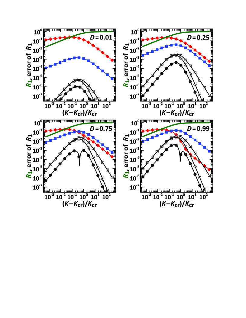
Figure 2: The accuracy of solutions for the noisy Kuramoto ensemble vs coupling strength $K$ is plotted with blue solid squires for the Ott-Antonsen ansatz (20), red solid diamonds for the Gaussian approximation (21), black open squares for the 2C truncation with closure $\varkappa_{3}=0$ (22), black open circles for closure $\varkappa_{3}=1.5\varkappa_{2}^{2}Z_{1}^{\ast}$, black solid circles for closure $\varkappa_{3}=1.5\varkappa_{2}^{2}/Z_{1}$ (23) (the cusp at a large noise strength is due to the change of sign of the error). Bold solid lines: the exact solution for the order parameter $R_{1}$. Parameters are rescaled so that $\gamma+D=1$: noise intensity $D$ is specified in plots, $K_{\mathrm{cr}}=2(\gamma+D)=2$. The case of vanishing intrinsic noise corresponds to $D=0$, the case of identical natural frequencies (or extremely strong noise) corresponds to $D=1$.

First, we calculated the “exact” steady state of system (15) by solving it with 200 cumulants taken into account. Then we found the steady solutions of approximations (9), (12), (16,17), (16,18):

$$R_{1}^{2}=1-\frac{K_{\mathrm{cr}}}{K}\,,$$ (20)

$$R_{1}^{2}=\sqrt{1-\frac{K_{\mathrm{cr}}}{K}}\,,$$ (21)

$$R_{1}^{2}=\frac{1}{2}-\frac{3K_{\mathrm{cr}}}{4K}+\frac{\sqrt{(2K-K_{\mathrm{cr}})^{2}+16D(K-K_{\mathrm{cr}})}}{4K}\,,$$ (22)

$$R_{1}^{2}=2-\frac{3K_{\mathrm{cr}}}{2K}-\frac{\sqrt{4(K-K_{\mathrm{cr}})(K-2D)+K_{\mathrm{cr}}^{2}}}{2K}\,,$$ (23)

respectively; the approximation (16,19) yields a cubic equation for $R_{1}^{2}$ with a cumbersome analytical solution. The deviations from the exact state are shown in Fig. 2. One can see, that the Gaussian approximation yields better accuracy than the OA ansatz only for strong noise ($D=0.99$, we remind that according to the normalization adopted $0\leq D\leq 1$) and strong coupling. The 2C approximation with the closure $\varkappa_{3}=0$ works as a plain first-order correction to the OA solution. The 2C approximation with the closure $\varkappa_{3}=(3/2)\varkappa_{2}^{2}/Z_{1}$ (18) is the best one in all situations. The 2C approximation with the closure $\varkappa_{3}=(3/2)\varkappa_{2}^{2}Z_{1}^{\ast}$ (19) is approaching the one with (18) for high synchrony, but yields the same accuracy as the closure $\varkappa_{3}=0$ for small $R_{1}$; for a strong noise and moderate synchrony, it is only slightly less accurate than the Gaussian approximation. Close to the synchronization threshold $K_{\mathrm{cr}}$, the inaccuracy of the Gaussian approximation reaches $0.2$ and exceeds the value of order parameter $R_{1}$, while the inaccuracy of $R_{1}$ with the OA ansatz is always reasonably small.

As the 2C approximations are based on the correction to the OA one, the former are always superior to the latter. One can also see, that the Gaussian approximation is accurate where the synchrony is high, which is also suggested by the von Mises distribution with $|h|\gg D$. Noteworthy, for high synchrony, the 2C approximations with closures (18) and (19) contain the Gaussian distribution as an admissible particular case. Moreover, these 2C truncations employ the Gaussian scaling only in the expression for the third cumulant $\varkappa_{3}$, while the second cumulant $\varkappa_{2}$ is allowed to deviate from the value dictated by the first cumulant $Z_{1}$ for the Gaussian distribution. Hence, these truncations also encompass a first-order correction for the case of Gaussian approximation under high synchrony. The closure (18) decently approximates the wrapped Gaussian distribution also for non-high synchrony. Being not less accurate than the first-order corrections to both the OA and Gaussian reductions, the 2C reduction with closure (18) becomes superior to them for the Kuramoto model with intrinsic noise.

V.2 Active rotators model

Figure 3: The difference between the exact steady-state solution for the population of noisy active rotators with Kuramoto-type coupling (3) and different approximations vs the coupling strength $K$. Blue solid squares: the OA ansatz (9); red solid diamonds: the Gaussian ansatz (12); black open squares: the two-cumulant reduction (16) with closure (17); black open circles: reduction (16) with (19); black solid circles: reduction (16) with (18). Bold solid lines: the order parameter $R_{1}$ for the accurate solution. Parameters: $\omega_{0}=1$, $a=3$, noise intensity $D$ is specified in the panels.

A population of active rotators with the Kuramoto-type coupling (3) can exhibit diverse regimes of collective dynamics, depending on parameter values Zaks-etal-2003 . Following Ref. Zaks-etal-2003 , we consider identical elements ($\gamma=0$) and focus on the case which is impossible for the Kuramoto ensemble: an excitable state of individual elements, $a>\omega_{0}$. Noteworthy, in this case the synchrony imperfectness is owned solely by intrinsic Gaussian noise. For all the cases presented in Figs. 3 and 4, the accurate solution is calculated from system (15) with $200$ cumulants. In Fig. 3, we evaluate accuracy of approximations (9), (12), (16,17), (16,18), and (16,19). For high synchrony (which is observed for a weak noise), the Gaussian approximation is more accurate than the OA one. Where the OA approximation fails, the plain 2C approximation with closure $\varkappa_{3}=0$ is not more accurate than the OA solution: in Fig. 3 for $D=0.01$ and $0.1$, the inaccuracy of the OA solution is of the same order of magnitude as the deviation of $R_{1}$ from $1$ for the exact solution. The 2C approximations with Gaussian closures always provide much better accuracy than both the OA and the Gaussian ones.

V.3 Testing scaling laws

In Fig. 4 we test how well the scaling laws (8) and (10), which lie at the basis of the OA and the Gaussian approximations, are valid. To check the OA ansatz (8), we plot the values of the cumulants: the cumulants $\varkappa_{n}$ with $n\geq 2$ should vanish if the OA ansatz is exact. To check the Gaussian approximation, we compare the $n$-dependence of $R_{n}=|Z_{n}|$ with a parabola.

Panel Fig. 4(a) shows the scaling for the Kuramoto model. One can see that although high-order cumulants do not vanish, there is a gap between the first and the second cumulants. This means that the OA ansatz is relatively good, but can be definitely improved by taking into account the second cumulant. The Gaussian approximation is valid for small $n\lesssim 7$ only.

Figure 4: The scaling law for the Kuramoto-Diado order parameters $R_{n}$ (circles) and the hierarchy of smallness for the circular cumulants $\varkappa_{n}$ (squares) are plotted for the noisy Kuramoto system with $D=0.75$, $\gamma=0.25$, $K=3K_{\mathrm{cr}}$ (a) and the population of active rotators with $\omega=1$, $a=3$, $K=1$, $\gamma=0$, $D=0.01$ (b) and $D=1$ (c). The solutions of system (15) are calculated with $200$ cumulants. Dotted lines show the trends $R_{n}\sim R_{1}^{n^{2}}$ and $\varkappa_{n}\propto{s^{2(n-1)}}$.

Panels Fig. 4(b,c) show the cumulants and the moments for the active rotator model. In panel (b) we illustrate the situation where the Gaussian approximation is superior to the OA one. One can see that the system practically perfectly obeys the $n^{2}$-scaling law for $R_{n}$. On the other hand, the gap between the first and the second cumulants is not large, which means that the OA ansatz is poor (see Fig. 3 for $D=0.01$, $K=1$); the inaccuracy of the OA solution is compatible to the deviation of $R_{1}$ from $1$. The case in panel (b) is the case of high synchrony. The plots in panel (c) are similar to those in panel (a); here only a few first values $R_{n}$ follow the $n^{2}$-scaling law (10). On the other hand, the gap between the first and the second cumulants is present, and the OA ansatz becomes acceptably accurate (see Fig. 3 for $D=1$, $K=1$); here the inaccuracy of the OA solution is one order of magnitude smaller than the deviation of $R_{1}$ from $1$.

Remarkably, in all the cases one observes that higher cumulants decay exponentially $\varkappa_{n}\propto\exp[-\mathrm{const}\,n]$. This law has been derived in Ref. Tyulkina-etal-2018 for small $D$ only; here we see that it is valid for moderate and strong noise as well. For a strong noise, there is a small parameter $(1/D)$ which can serve for a hierarchy in the system, $\varkappa_{n+1}\sim(1/D)\varkappa_{n}$. For a moderate noise strength, there is no small parameter, but nevertheless, a hierarchy is present.

Table 1: Low-dimensional model reductions

Reduction	Eqs.	Comments
OA ansatz (9) Gaussian approximation (12)		The Gaussian approximation is superior to the OA one for high synchrony, if the distortion of the perfect synchrony is not dominantly due to a non-Gaussian disorder (e.g. Lorentzian distribution of natural frequencies).
Two-cumulant reduction with $\varkappa_{3}=0$	(16,17)	This plain first-order correction to the OA solution is frequently superior to the Gaussian approximation, but may have the same (low) accuracy as the OA ansatz, where the latter completely fails.
Two-cumulant reduction with $\varkappa_{3}=\frac{3}{2}\varkappa_{2}^{2}/Z_{1}$	(16,18)	It works as a first-order correction to the best of OA and Gaussian approximations. Not to be used for problems where $Z_{1}$ can approach $0$ without $\varkappa_{2}^{2}/Z_{1}$ remaining finite.
Two-cumulant reduction with $\varkappa_{3}=\frac{3}{2}\varkappa_{2}^{2}Z_{1}^{\ast}$	(16,19)	For high synchrony, its accuracy approaches the accuracy of closure $\varkappa_{3}=\frac{3}{2}\varkappa_{2}^{2}/Z_{1}$. For low synchrony, it is as accurate as the plain two-cumulant truncation ($\varkappa_{3}=0$).

VI Conclusion

We have compared five low-dimensional approximations describing the dynamics of large populations of noisy phase oscillators (or active rotators) with global sine-coupling: Eqs. (9), (12), (16,17), (16,18), and (16,19); the latter two cases are novel two-cumulant truncations within the framework of circular cumulant formalism. As prototypic examples, we have chosen the standard Kuramoto model and the active rotator model in the excitable state regime. Tabel 1 summarizes applicability of different low-dimensional reductions. The truncation with the closure according to $\varkappa_{3}=(3/2)\varkappa_{2}^{2}/\varkappa_{1}$, which most accurately corresponds to the Gaussian reduction under high synchrony, deserves special attention. By construction, this truncation is simultaneously a first-order correction to the Ott-Antonsen ansatz, and comprises the wrapped Gaussian distribution of phases, where the latter can be formed. In all the cases considered, this two-cumulant approximation is significantly superior to all other approximations. Remarkably, even for the cases, where $R_{n}$ nearly perfectly follows the $n^{2}$-scaling law, this two-cumulant approximation enhances the accuracy of the Gaussian one, by a few orders of magnitude.

Generally, a high synchrony is not a sufficient condition for applicability of the Gaussian ansatz. In this paper, our analysis has been restricted to the situations of synchronization by coupling. However, for synchronization by a common noise Pikovsky-1984b ; Teramae-Tanaka-2004 ; Goldobin-Pikovsky-2004 , in nonideal situations (i.e., with intrinsic noise and/or nonidentity of elements), it is known that the phase distribution possesses heavy power-law tails even in the limit of high synchrony Goldobin-Pikovsky-2005b ; Pimenova-etal-2016 . For such systems, the Gaussian ansatz is never natural.

- (1) A. Pikovsky, M. Rosenblum, and J. Kurths, Synchronization: A Universal Concept in Nonlinear Sciences (Cambridge University Press, Cambridge, 2001, 2003).
- (2) S. Strogatz, Sync (Hyperion, 2003).
- (3) G. Filatrella, A. H. Nielsen, and N. F. Pedersen, Analysis of a power grid using a Kuramoto-like model, Eur. Phys. J. B 61, 485–491 (2008).
- (4) A. T. Winfree, The Geometry of Biological Time (Springer, 2001).
- (5) J. A. Acebrón, L. L. Bonilla, C. J. P. Vicente, F. Ritort, and R. Spigler, The Kuramoto model: A simple paradigm for synchronization phenomena, Rev. Mod. Phys. 77, 137–185 (2005).
- (6) A. Pikovsky and M. Rosenblum, Dynamics of globally coupled oscillators: progress and perspectives, Chaos 25, 097616 (2015).
- (7) E. Ott and T. M. Antonsen, Low dimensional behavior of large systems of globally coupled oscillators, Chaos 18, 037113 (2008).
- (8) K. M. Hannay, D. B. Forger, and V. Booth, Macroscopic models for networks of coupled biological oscillators, Sci. Adv. 4, e1701047 (2018).
- (9) M. A. Zaks, A. B. Neiman, S. Feistel, and L. Schimansky-Geier, Noise-controlled oscillations and their bifurcations in coupled phase oscillators, Phys. Rev. E 68, 066206 (2003).
- (10) B. Sonnenschein and L. Schimansky-Geier, Approximate solution to the stochastic Kuramoto model, Phys. Rev. E 88, 052111 (2013).
- (11) B. Sonnenschein, Th. K. DM. Peron, F. A. Rodrigues, J. Kurths, and L. Schimansky-Geier, Collective dynamics in two populations of noisy oscillators with asymmetric interactions, Phys. Rev. E 91, 062910 (2015).
- (12) I. V. Tyulkina, D. S. Goldobin, L. S. Klimenko, and A. Pikovsky, Dynamics of Noisy Oscillator Populations beyond the Ott-Antonsen Ansatz, Phys. Rev. Lett. 120, 264101 (2018).
- (13) A. S. Pikovskii, Synchronization and stochastization of array of self-excited oscillators by external noise, Radiophys. Quantum Electron. 27, 390 (1984).
- (14) J. N. Teramae and D. Tanaka, Robustness of the Noise-Induced Phase Synchronization in a General Class of Limit Cycle Oscillators, Phys. Rev. Lett. 93, 204103 (2004).
- (15) D. S. Goldobin and A. S. Pikovsky, Synchronization of periodic self-oscillations by common noise, Radiophys. Quantum Electron. 47, 910 (2004).
- (16) D. S. Goldobin and A. Pikovsky, Synchronization and desynchronization of self-sustained oscillators by common noise, Phys. Rev. E 71, 045201(R) (2005).
- (17) A. V. Pimenova, D. S. Goldobin, M. Rosenblum, and A. Pikovsky, Interplay of coupling and common noise at the transition to synchrony in oscillator populations, Sci. Rep. 6, 38518 (2016).