Verifying and Reporting Fast Radio Bursts

Abstract

Fast Radio Bursts (FRBs) are a class of short-duration transients at radio wavelengths with inferred astrophysical origin. The prototypical FRB is a broadband signal that occurs over the extent of the receiver frequency range, is narrow in time, and is highly dispersed, following a $\nu^{-2}$ relation. However, some FRBs appear band-limited, and show apparent scintillation, complex frequency-dependent structure, or multi-component pulse shapes. While there is sufficient evidence that FRBs are indeed astrophysical, their one-off nature necessitates extra scrutiny when reporting a detection as bona fide and not a false positive. Currently, there is no formal validation framework for FRBs, rather a set of community practices. In this article, we discuss potential sources of false positives, and suggest a framework in which FRB-like events can be evaluated as real or otherwise. We present examples of false-positive events in data from the Arecibo, LOFAR, and Nanshan telescopes, which while FRB-like, are found to be due to instrumental variations, noise, and radio-frequency interference. Differentiating these false-positive detections from astrophysical events requires knowledge and tests beyond thresholded single-pulse detection. We discuss post-detection analyses, verification tests, and data sets which should be provided when reporting an FRB detection.

1 Introduction

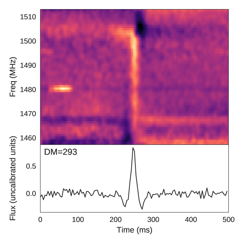
(a)

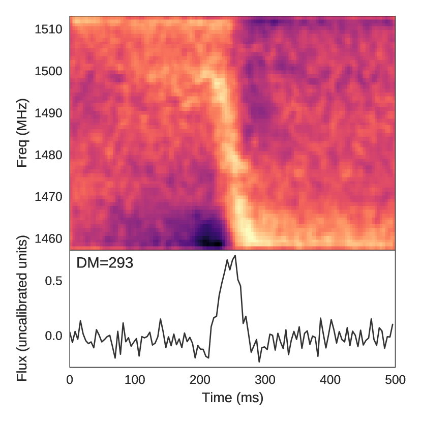
(b)

Figure 1: Dynamic spectrum (top) and S/N-maximized de-dispersed time series (bottom) of an FRB-like event that was detected simultaneously in Beam 0 and 5 of the ALFA receiver on December 4, 2016. The dynamic spectrum has been bandpass normalized. (a) Detected FRB-like event in Beam 0 of ALFA. The characteristic dip before and after the event is due to zero-DM removal which is part of the ALFABURST RFI exciser. The strong, narrow band source at 1480 MHz around 100 ms is due to a local RFI source. (b) Same event detected in Beam 5.

The astrophysical origin of Fast Radio Bursts (FRBs) has been a mystery since they were first reported (Lorimer et al., 2007). Though, the detection of multiple FRBs in Thornton et al. (2013) put forth a convincing case for their astrophysical nature and, subsequent detections have re-enforced this case. The Dispersion Measure (DM) associated with the reported events indicate they occur well beyond our Galaxy, possibly at cosmological distances. Given their extragalactic distance, observed fluxes suggest extremely energetic progenitors; however, their emission mechanism remains unknown. The consensus that FRB are astrophysical events developed from detections with multiple telescopes, over multiple wavelengths, using different receiver systems. FRBs are difficult to detect as they require high-gain telescopes which typically have a small field of view, such that despite many thousands of observing hours, only a few dozen have been reported as of this writing (Petroff et al., 2016).

The prototypical FRB is broad-band across the observable bandwidth of the receivers used. The pulse is narrow-in-time—on the order of a few milliseconds in width—and highly dispersed, exhibiting a $\nu^{-2}$ relation with frequency. Despite follow-up observations in the direction of FRB events, only FRB  121102 has been shown to repeat (Spitler et al., 2016). Several reported detections deviate from this prototypical form, exhibiting complex frequency-dependent structure and are possibly band-limited. The pulse width also varies, due to either the emission process or propagation effects such as scattering from the Interstellar Medium (ISM) and Intergalactic Medium (IGM).

These rare events are detected by automated, high-performance software pipelines that extensively search a broad range of trial DMs and pulse widths (Barsdell et al., 2012; Karastergiou et al., 2015; Bannister et al., 2017; The CHIME/FRB Collaboration et al., 2018). Each de-dispersed time series is then thresholded – any peaks above a minimum S/N are reported as candidates. The number of candidates is usually overwhelming due to Radio-frequency Interference (RFI) and system gain variations. Initially, candidates were reviewed manually; however, with the amount of data acquired in recent surveys, it has become a significant time effort to do so. As such, and as our understanding of the expected signal properties has grown, so too has the use of machine-learning-based classifiers of candidate events (e.g. Wagstaff et al., 2016; Foster et al., 2018; Farah et al., 2018; Connor & van Leeuwen, 2018).

As FRBs are rare and appear not to repeat (with the notable exception of FRB 121102), being able to confidently verify them is an important issue. There is significant RFI detectable at all radio observatories, and there are known anthropogenic sources that appear FRB-like (Petroff et al., 2015b). Given the significant number of DM trials and high-time resolution of the spectra in a typical survey, there are a large number of false-positives (type-I errors) that pass the automated post-processing detection thresholds. This is by design, as we would like to severely limit the potential for false-negatives (type-II errors) in our detection pipelines by accepting a number of false-positives during automated searches and manually discarding them later. But, given the large sampling of the parameter search space it can be difficult to differentiate between a true, astrophysical FRB (true-positive) and a ‘terrestrial FRB’ (false-positive) due to RFI, systematics, or other local effects. As the survey time increases, the likelihood of detecting such a false-positive will increase.

In this paper, we present a list of verification criteria to counter false detection of ‘terrestrial FRBs’, that can be applied post facto to recorded data. We firstly discuss examples of FRB-like sources, which after investigation, were shown to be non-astrophysical (§ 2). Using these and previously reported FRBs, we develop a set of criteria to test detections against (§ 3). We then apply these criteria to some of the previously reported detections (§ 4) as examples of usage, then discuss future observational methods to reduce ambiguity (§ 5). We conclude with suggestions as to what data, in addition to the detected dynamic spectrum, should be reported to provide a robust statement about FRB detections in general.

2 False-Positive FRB Detections

The rate of false-positive detections is set by the minimum S/N threshold, the parameter search space, and the terrestrial environment of the observatory. We use the term ‘terrestrial’ to encompass multiple effects: anthropogenic radio signals and variations in the observing system.

Most potential false-positive events are flagged using filters and classifier models. The remaining events are commonly examined by eye as expert human knowledge appears to be the best way to classify a detection. However, time constraints do not allow for all events to be classified in this way. On inspection, true astrophysical events and terrestrial events can be difficult to differentiate between, even by the expert eye. This is not surprising, as they have passed the detection pipeline thresholds.

Studies of the telescope state during detection, can often assist in determining the origin of an event. Nonetheless, ambiguities can remain. In this section we present examples of such events—which on initial inspection appear astrophysical, but after further investigation prove terrestrial in origin.

2.1 ALFA Terrestrial FRB Candidate

In the two years of the initial ALFABURST survey (Chennamangalam et al., 2017; Foster et al., 2018), over 200,000 8.4-second data windows were recorded in which the FRB search pipeline detected candidates using a minimum S/N detection threshold of 10. The vast majority of these events were due to RFI and instrumental variations, while others were due to bright single pulses of known pulsars. The random forest-based classifier model outputs an ordered list of events based on the likelihood of the event being a pulse.

A narrow-in-time, broad-in-frequency, millisecond pulse was detected with the ALFABURST system at 09:31:06 Arecibo local time (UTC 13:31:06) on 2016, December 4 in Beam 0 (the central beam) of the Arecibo L-Band Feed Array (ALFA) receiver (Figure 1(a)) which we label as the D20161204 event for this discussion. ALFABURST was processing 56 MHz of bandwidth between 1457 MHz and 1513 MHz. The S/N of this pulse is maximized when the pulse is de-dispersed with a DM of 293 pc cm^-3, and the native 256 $\mu$s time resolution is decimated by a factor of 16 to a time resolution of 4.096 ms. The de-dispersed time series shows an approximately 20 ms Full-Width at Half-Maximum (FWHM) pulse. The dip before and after the pulse is due to the zero-DM filtering (i.e. the moving channel average is subtracted) before pulse detection (Eatough et al., 2009). This is a simple way to remove a drifting gain baseline at the cost of removing some of the overall pulse power, particularly at low DM trials.

On initial inspection, this event appears astrophysical. From radiometer noise considerations, the flux density of the pulse is

$$S=\textrm{SEFD}\frac{\textrm{S/N}}{\sqrt{D\;\Delta\tau\;\Delta\nu}}$$ (1)

where SEFD is the system-equivalent flux density of the telescope, $\Delta\tau$ is the time resolution of the spectra, $\Delta\nu$ is the total frequency bandwidth of the spectra, and $D$ is the time decimation factor which maximizes the S/N of the detections. Adopting a System Equivalent Flux Density (SEFD) of 3 Jy for the ALFA receiver, results in $S=66$ mJy from beam 0, which would be lower than what has been observed for any previously detected FRBs (Petroff et al., 2016). However, this flux estimate is a lower limit, assuming the source is at the center of the beam. The pulse width is large for an FRB but within the range of those previously reported.

As ALFA is a multi-beam system, we checked if the event occurred in any other beams. Of the six other ALFA beams, the event also appears in beam 5 (Figure 1(b)), which is adjacent to beam 0. This pulse lines up with the beam 0 event in time exactly, but the event S/N was maximized ($S/N=16$) for a DM of 829 pc cm^-3, but this higher DM is due to a slope in the bandpass. Flattening the bandpass, and re-performing the DM-trial fit, resulted in a S/N-maximized DM closer to that of beam 0. Our RFI clipping method was applied during this event which is known to affect the pulse shape, and generally results in a maximized S/N at a higher DM trial than expected. We thus conclude that the Beam 0 and Beam 5 event are the same event.

We checked if any other events occurred with in a larger time window of the detection, as the event could be a high S/N detection of a series of RFI events. In the immediate period before and after the pulse, there are no similar events (Figure 2). The event appears to be isolated in time, with a fairly compact representation in DM-time space (Figure 2(a)) similar to that of a single pulse from a high DM pulsar, such as PSR B1859+03 (Figure 2(b)).

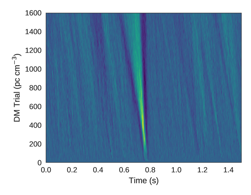
(a) DM vs. time plot of for a 1.5 second window centred on the December 4th event in Beam 0. The S/N peaks at a DM of 293 pc cm^-3. There is a significant detection at larger DM trials due to the width of the pulse.

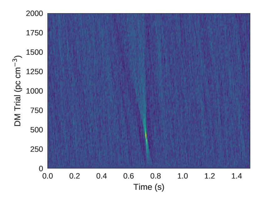
(b) DM vs. time plot of a bright single pulse from PSR B1859+03 which has a DM of 402 pc cm^-3 and pulse width of 11 ms (W50).

Figure 2: DM-space plot shows the characteristic butterfly pattern of the narrow-in-time, dispersed pulse detected by ALFABURST at a different epoch. A single pulse detection of PSR B1859+03 is shown for reference.

As ALFABURST is a commensal observing program we checked the telescope pointing, state, and receiver stability. The telescope pointing was fixed in azimuth and elevation, corresponding to a fixed declination (+15:11) and drifting in RA (event detected at RA=14:42). No known pulsar or Rotating Radio Transient (RRAT) with a similar DM lies within the beam primary lobe of this pointing.

The telescope logs provide the first indication that this event is spurious. As ALFABURST is a commensal observation survey the search pipeline regularly checks the status of the receiver turret and the centre observing frequency. ALFA was logged as active and the centre observing frequency remained unchanged during this time, but the turret was in a different position than where ALFA should be if it were at the secondary focus.

The observing schedule for the morning of December 4, was project P3080 using ALFA to perform an FRB survey of the Virgo cluster until 09:00 local time, followed by Project R3037, an S-Band radar observation. The event occurred during a time of no active observation with ALFA active but in the wrong turret position. Thus, ALFA was at a significantly reduced sensitivity than expected when in the correct position.

As the telescope was in an inactive observing state we checked if the electronics were operating as expected during normal ALFA observations. The average bandpass of Beam 0 and Beam 5 during the time of the event shows that the shape and system noise appear atypical compared to normal observations (Figure 3). Beam 0 and 5 bandpasses appear similar and have overlapping narrow-band features at 1468, 1480, 1496, and 1504 MHz due to the settling of Phased-locked Loop (PLL) in a local oscillator associated with an on-site RFI monitor. The system noise appears higher during the event, which leads to smoother bandpasses than typical. In the detection pipeline the data are normalized, which removes all absolute scaling. This indicates that the SEFD is too low in our flux calibration. This increase in system noise is due to the change in turret position, causing the ALFA feed to pick up reflections from other equipment in the dome, and the dome itself as a warm source. This event is most likely due to the analogue electronics becoming non-linear from this increase in system noise.

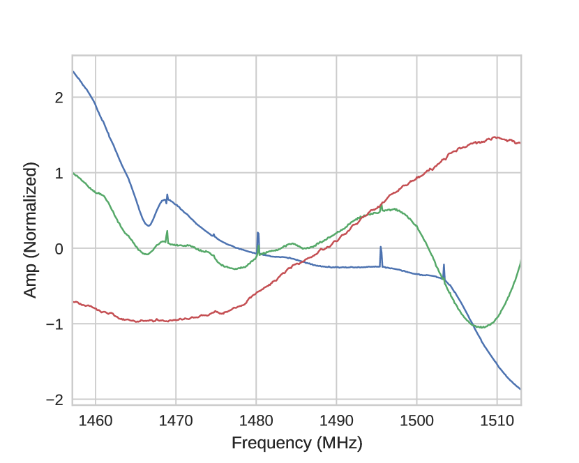
Figure 3: Average bandpass response during the December 4, 2016 event for Beam 0 (green) and Beam 5 (blue). A typical bandpass (red) is plotted for reference. The narrow features at 1468, 1480, 1496, and 1504 MHz is due to local RFI. These bandpasses have been normalized in the detection pipeline.

Evidence for analogue gain variations is further justified by considering the data over a larger time window. Approximately 80 seconds before the event, frequency-varying structure across the band (top of Figure 4) was present. Though not as narrow-in-time as the event, they appear related to the same phenomenon. The DM$-$time plot (bottom of Figure 4) shows that much of the structure would be detected as dispersed pulses. In particular, at around the four second mark the structure would result in a wide-in-time, highly dispersed pulse detection. The structure immediately proceeding it would be detected as a negatively dispersed pulse, but only positive DM candidates are recorded. The narrow-in-frequency, repeating feature present at 1467 MHz is the same feature as seen in the time-averaged bandpass (Figure 3).

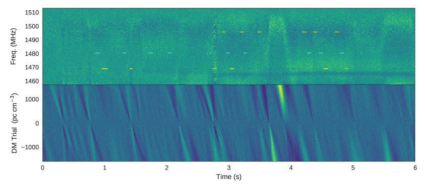
Figure 4: Dynamic spectrum (top) and DM-time plot (bottom) of 6 seconds from beam 0 approximately 80 seconds before the D20161204 event. The dynamic spectrum shows frequency evolution of the bandpass as a function of time (e.g. the sinusoidal shape around the four second mark) results in significant detections across the trial DM range -1600 to 1600 pc cm^-3. The narrow-band RFI at 1467 MHz is due to a local RFI source. The broad-band pulse near the three second mark is an RFI source which has been partially removed.

In isolation, and taking into account the one-off, transient nature of FRBs, the initial beam 0 detection reasonably appears astrophysical. But, after further checks on the telescope state and examining data across a larger time window (several seconds) around the event, we can confidently classify this event as terrestrial. This has motivated us to develop a set of tests to use in verifying an event as astrophysical, this is discussed in detail in Section 3.

2.2 Low-S/N False-Positive Detections

While the D20161204 event (Section 2.1) is a rare false-positive detection based on a unique telescope state, low-S/N false-positive candidates occur regularly. For example, on July 30, 2015 an apparently 10-$\sigma$ event with a DM of 1370 pc cm^-3 was detected (Figure 5) by the ALFABURST pipeline in beam 5. The pulse can barely be seen in the dynamic spectrum, but in the DM-time plot, there is a compact peak centered at a DM of 1370 pc cm^-3 with no other similar events apparent. After re-analysis of the dynamic spectrum noise, this event only has an S/N $\sim$6, but was reported as a higher S/N because of the data window size used to calculate the system noise. Locally in time, there is an increase in system noise, leading to a reduced S/N. This is not an uncommon event and many of these events have no immediate explanation.

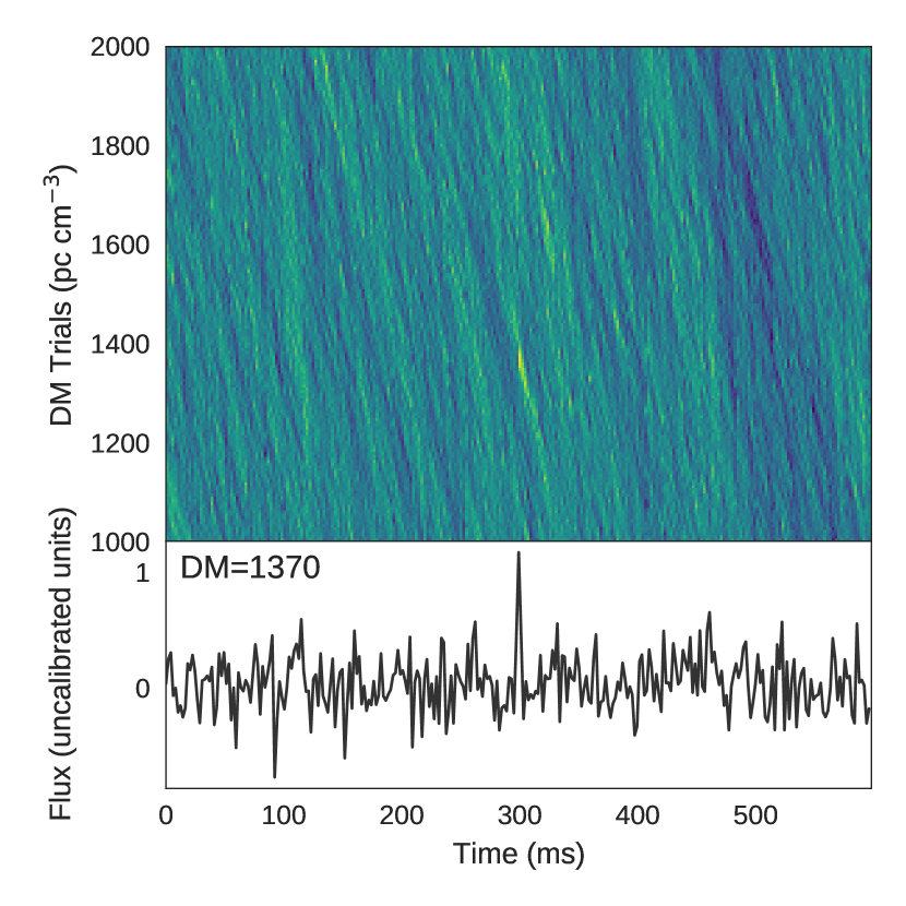
Figure 5: DM-space plot and time series of a high DM event with reported S/N above 10-$\sigma$ on July 30, 2015. After re-analysis and review of the telescope meta-data it was determined that this event was due to local system noise.

These types of events prove to be difficult to validate as either astrophysical or terrestrial. The choice of minimum S/N is partially set by the willingness of the observers to sort through false-positive events. There are likely many low-S/N FRBs that are either not detected at all or labelled as false-positive events. The reported detection of a pulse from FRB 121102 with APERTIF (Oostrum et al., 2017) had an S/N $\approx 4$. In a blind survey across different sky positions and trial DMs, this would not be a significant detection. But, the sky position and S/N-maximized DM of the repeating FRB 121102 is known, thus a lower S/N detection may be sufficient.

2.3 ARTEMIS Radar Detection

ARTEMIS (Karastergiou et al., 2015) is a low-frequency FRB survey using the Rawlings Array, the LOFAR-UK station at Chilbolton Observatory. The survey uses a similar fractional bandwidth ($\sim 0.04$) to ALFABURST, but is centered at 145 MHz. In this survey, known pulsars regularly transit the beams that are fixed in azimuth and elevation, and single pulses are routinely observed. An RFI excision algorithm has been developed for this survey that successfully removes the majority of false-positive events. Over many thousands of observing hours, rare events occasionally pass this filter.

A particularly interesting event for which the S/N was maximized at a DM of 85 pc cm^-3 is shown in Figure 6. Though this event has a low DM compared to the reported FRBs, this still proves to be a relevant example as discussed later in this section. The narrow-in-time pulse can be seen in the dynamic spectrum at frequencies above 146 MHz, but not at lower frequencies where it could be hidden by narrow band RFI. The de-dispersed time series shows a high-S/N detection of a pulse of approximately 20 ms in width. The beam pointing during the time of the event is not associated with any known pulsar or RRAT around a DM$\sim$85 pc cm^-3.

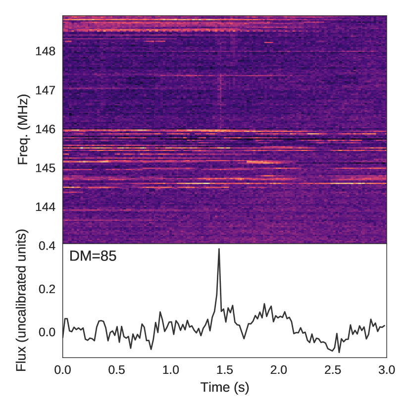
Figure 6: A dispersed pulse detected by the automated ARTEMIS search pipeline at the LOFAR-UK station. The S/N is maximized when the signal is dedispersed to a DM of 85 pc cm^-3. The dynamic spectrum has a time resolution of 20 ms and frequency resolution of 3 kHz.

Plotting the event in DM-time space across the ARTEMIS DM range ($0-320$ pc cm^-3, Figure 7) shows a strong, compact detection as expected of a dispersed pulse. But, the apparent limited bandwidth of the pulse means that the pulse does not necessarily follow a $\nu^{-2}$ dispersion relation.

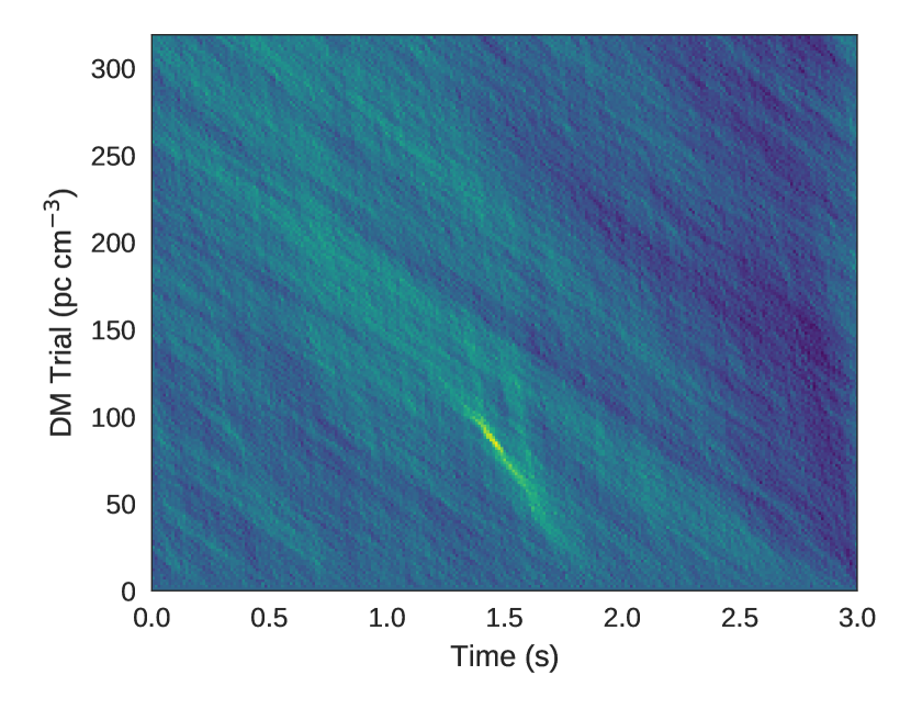
Figure 7: DM-space plot over the DM trial range of the ARTEMIS survey. A strong, compact detection occurs at a DM of 85 pc cm^-3 with no other apparent events during the time.

The ARTEMIS search pipeline, like most FRB search pipelines, decimates the dynamic spectrum in time to search over a range of pulse widths. The S/N of the event shown in Figure 6 is maximized for a time decimation factor of 64. With a native resolution of $327.68~{}\mu s$, this results in a decimated time resolution of 20 ms. At this resolution, the pulse appears to be a continuous broadband pulse. When an event is detected in the pipeline, the dynamic spectrum is saved at the original resolution. Plotting at 1 ms time resolution (Figure 8), the repeating nature of a linear frequency-modulated signal used for pulse compression in radar can be seen.

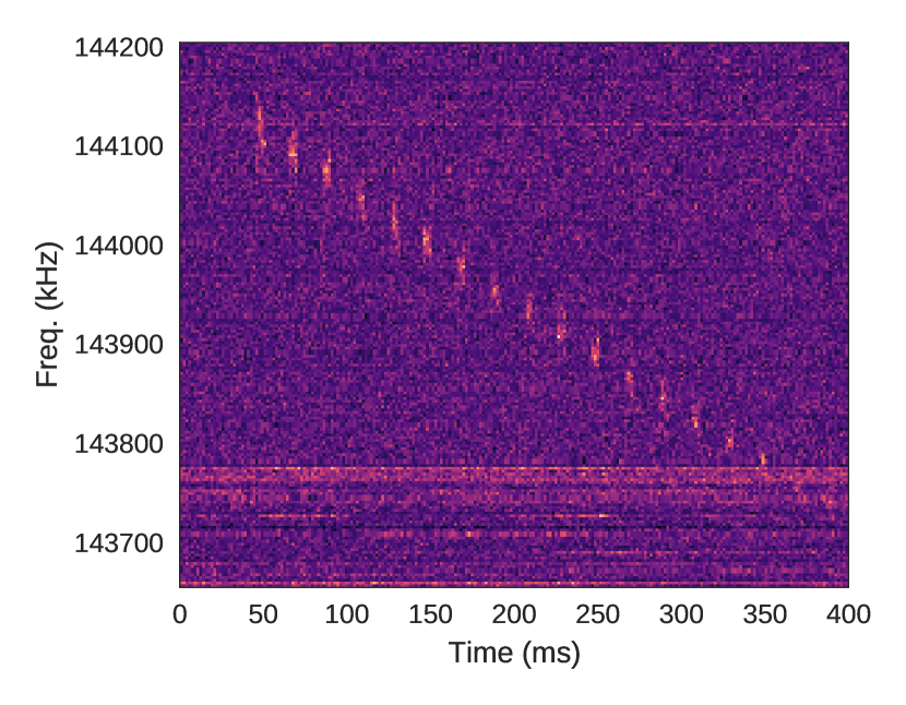
Figure 8: A zoomed in view of the event in Figure 6 at high time (1 ms) and frequency (1.5 kHz) resolution shows the distinct pattern of a linear frequency-modulated radar pulse.

In radar signals, the bandwidth of the transmitter provides information on the range and direction of a target. A narrow-band radar transmitter can be used to approximate a dispersed, wide-band pulse by modulating the frequency of the transmitted pulse. The narrow-band (in frequency) pulse is stepped in frequency across a transmission band. Between each step the pulse is not transmitted, resulting in the gaps in time between pulses, such as in Figure 8. An increase in the delay between the narrow-band pulses will result in a more dispersed wide-band pulse.

Linear frequency-modulation is the most typical form of chirp compression, but non-linear methods are also used. Such a modulation technique may be the origin of other detected signals (see next section). There are a number of allocated radar usages in the LOFAR observing band which could be the source of the observed radar pulse (Ofcom, 2017). Radar is used from UHF to C-band (300 MHz – 8 GHz), covering a wide range of frequencies at which FRB surveys operate. We could not determine the exact origin of the radar pulse, since radar is used for commercial and military purposes, most of these signal specifications, modulations, and source locations are proprietary.

As the radar signal can resemble a dispersed pulse, we expect to detect such signals with FRB pipelines. Verification of this event is straightforward when the high-time and frequency resolution data are available to reveal the narrow-band, pulsed nature of the event.

2.4 XAO Repeating Event

The 25-m Nanshan Telescope at Xinjiang Astronomical Observatory (XAO) is currently running an FRB survey which covers over 300 MHz at L-band (1 – 2 GHz), sampling at $64\;\mu s$ resolution. On November 18, 2016 hundreds of bright, dispersed pulses were detected. The pulses varied in S/N, but had the same S/N-maximized DM of 531.8 pc cm^-3. The pulses show a distinct double peak (each peak $\sim 2$ ms wide) separated by $\sim 3$ ms (Figure 9). The pulses are only apparent in a portion of the band.

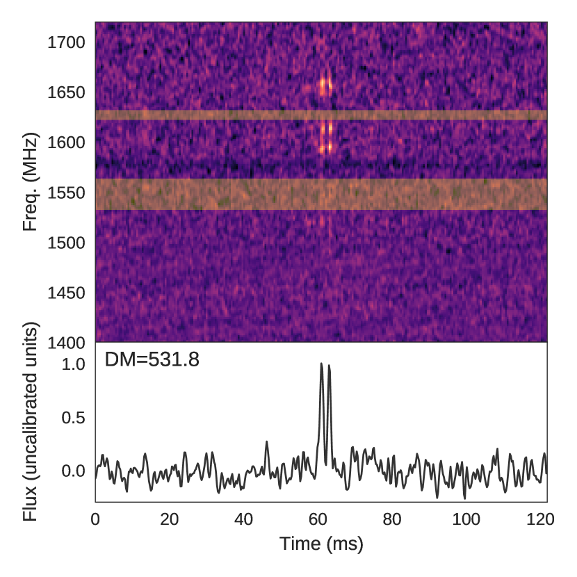
Figure 9: Example of a detected pulse with the Nanshan Radio Telescope at XAO which is S/N maximized at a DM of $531.8$ pc cm^-3. Hundreds of such pulses were detected over a period of a few hours. The orange bars represent regions that have had significant constant-in-time RFI replaced by noise.

A periodicity search revealed a periodicity of $\sim 1.7$ s, but the timing residuals were orders of magnitude higher ($\sim 0.01$ s) than that of a typical pulsar periodicity. Further, the pulses were seen at different pointings across the sky. Most were detected at a low altitude pointing angle, but some were detected close to zenith. Dispersion in these pulses was found to deviate from a $\nu^{-2}$ relation by $1.5\sigma$. A dispersed astrophysical source should always follow a cold plasma $\nu^{-2}$ relation. This rules out a pulsar, or an astrophysical source in general.

A thorough search of possible local sources, such as new equipment, vehicles, and aircraft was performed, with no obvious candidate being found. Detection of multiple pulses at different beam pointings indicates the source may be directly illuminating the feed.

The Nanshan L-band receiver is a single pixel system. A multi-beam system, such as the Parkes 13-beam or ALFA 7-beam receivers, would likely have detected these events in several beams, which would indicate a terrestrial origin to the event.

Had only a single pulse been detected, for example if the source was weaker, or the telescope was only sensitive to the highest S/N event, it would be difficult to show that the event was due to RFI. Multiple reported FRBs, including the repeater FRB 121102, do not cover the entire observing band. This has been explained by various intrinsic or intermediate effects, e.g. scintillation (Masui et al., 2015; Spitler et al., 2018) and plasma lensing (Cordes et al., 2017). In the case of a single detected pulse, it would be reasonable to report it as an astrophysical FRB.

Since the initial detection of the pulses in November 2016 the pulses have not been re-detected. While the source is terrestrial in origin, these pulses present a situation where terrestrial sources can easily be misidentified as one-off astrophysical events. This event, along with the other events presented in this section should present a case for developing common criteria, observing strategies, and data recording to improve the confidence in FRB detections.

2.5 Parkes Perytons

A class of non-astrophysical, yet FRB-like signals were found in high-time resolution data around 1.4 GHz with the Parkes Telescope (Burke-Spolaor et al., 2011). These signals, dubbed ‘Perytons’, are dispersed in frequency like FRBs, but do not obey the $\nu^{-2}$ cold plasma relation. Initial reporting classified these signals as terrestrial as they occurred in the near-field (i.e. they appeared in most of the beams of the Parkes Multi-beam receiver at approximately equal S/N) indicating the source was local to the telescope site. Additional Perytons were detected while an on-site, broad-band RFI monitor recorded simultaneous RFI at $2.4$ GHz (Petroff et al., 2015b). Further analysis led to a time of day dependence relation that indicated they were generated by equipment in use during normal working hours. Ultimately, these were found to be a form of RFI generated by microwave ovens.

2.6 Simulated False-Positive Pulses

As shown in the examples of this section, narrow-in-time pulses from terrestrial origins can take multiple forms which follow an approximately $\nu^{-2}$ dispersion relation. This can be due to instrumentation variation effects, or as anthropogenically created signals such as chirps with frequency-modulated structure. An FRB dedispersion pipeline acts as an approximate matched filter to a subset of these signals leading them to be detected with high S/N. By simulating a simple receiver and dispersed pulse model we can show that FRB pipeline false-positive detections can be produced over a broad range of DMs and S/Ns.

We model this effect by simulating a number of dispersion and receiver models at L-band. Pulses are modelled with linear ($\nu^{-1}$), quadratic ($\nu^{-2}$), cubic ($\nu^{-3}$), and logistic ($(1+e^{-\nu})^{-1}$) functions which cover a bandwidth from $\nu_{\textrm{p,0}}=1300$ MHz to $\nu_{\textrm{p,1}}=1800$ MHz. The quadratic dispersion model is used as the reference, while the other dispersion models are simulated as they are similar to anthropogenic signals of known and unknown origin. Example pulses are shown in the top row of Figure 10. The time duration of the pulse $\Delta t_{\textrm{pulse}}$ is fixed such that the quadratically dispersed pulse has an S/N-maximized DM of approximately 1000 pc cm^-3. The pulse is convolved with a Gaussian function to give a pulse width $\Delta t_{\textrm{width}}$ of 3 ms. The amplitude of the pulse is set to unity across the extent of the band.

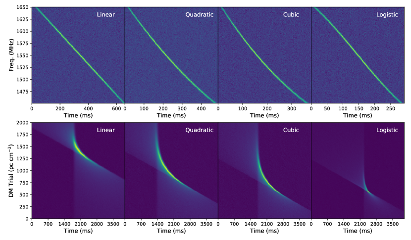
Figure 10: Top row: examples of simulated pulses with different dispersion relations: linear, quadratic, cubic, logistic (left to right). Bottom row: DM-space plots of the simulated pulses for a receiver model of $\Delta\nu_{\textrm{obs}}=200$ MHz centred at $\nu_{\textrm{obs,c}}=1550$ MHz. Initial starting time is arbitrary and different between plots.

A receiver model is used to simulate the observation. This model is parameterized by a central observing frequency $\nu_{\textrm{obs,c}}$, bandwidth $\Delta\nu_{\textrm{obs}}$, frequency resolution $\Delta\nu_{\rm chan}$, time resolution $\tau_{\rm int}$, and per channel noise $\sigma_{\textrm{chan}}$. The bandpass response is modelled as a Gaussian with width $\Delta\nu_{\textrm{obs}}$. A schematic of a simulated pulse and receiver model is shown in Figure 11. For the simulation, we sampled centre observing frequencies from 1400 MHz to 1700 MHz in 20 MHz steps and receiver bandwidths of 50, 100, and 200 MHz. The quadratically dedispersed pulses ranged in S/N from approximately 20–40 depending on $\Delta\nu_{\textrm{obs}}$. The time and frequency resolution of the data was $\tau_{\rm int}=256\,\mu\textrm{s}$ and $\Delta\nu_{\rm chan}=360$ kHz.

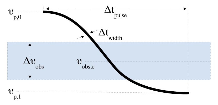
Figure 11: Logistic function pulse and receiver model used to simulate the response and S/N-maximized DM search. The pulse is modelled as a pulse of width $\Delta t_{\textrm{width}}$ that extends over a time period $\Delta t_{\textrm{pulse}}$, with a start $\nu_{p,0}$ and stop $\nu_{p,1}$ frequency beyond the bandwidth $\Delta\nu_{\textrm{obs}}$ of the receiver system centred at $\nu_{\textrm{obs,c}}$. An similar model was used for the linearly, quadratically, and cubically dispersed pulse models.

A DM search of these simulated pulses results in significant detections in compact regions of the DM trial space (bottom row of Figure 10). Each pulse was detected with similar S/N to that of the quadratically dispersed pulse using the same simulation parameters, but at different DMs (Figure 12). The S/N-maximized DM of quadratically dispersed pulse stays fixed across the choice of observing frequency as expected. Though, smaller observing bandwidths result in an increase in the S/N-maximized DM at lower frequencies due to the pulse width. The cubically dispersed pulse shows a similar flat response as the quadratically dispersed pulse but with a faster upturn in DM at lower $\nu_{\textrm{obs,c}}$. The S/N-maximized DM of the linearly dispersed pulse has a linear response as a function observing frequency, independent of observing bandwidth. The S/N-maximized DM of the logistically dispersed pulse varies significantly as a function of observing bandwidth and frequency. This is only a small set of simulated parameters and dispersion models, but a wide range of S/N-maximized DMs can be produced which appear similar to the quadratically dispersed pulse.

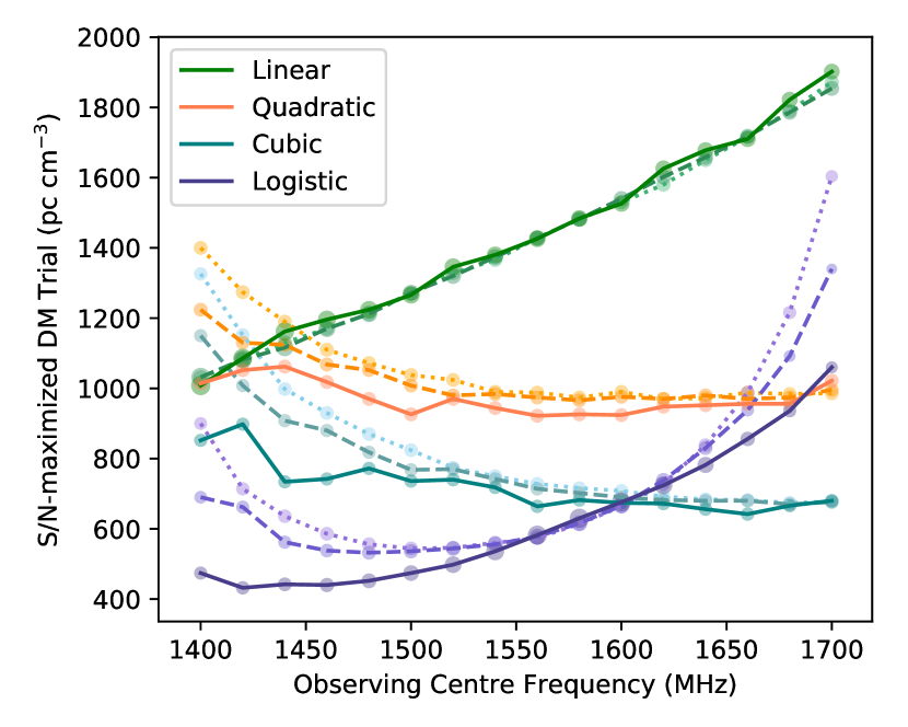
Figure 12: S/N-maximized DM trial for the simulation of pulses centred at 1550 MHz over a range of central observing frequencies. Pulses with linear (green), quadratic (orange), cubic (teal), logistic (purple) dispersion relations are simulated using a detection receiver with a bandwidth of 50 MHz (dotted), 100 MHz (dashed), 200 MHz (solid). The point size scales are the detection S/N relative to the quadratic pulse detection S/N.

If these pulses are detected with a high S/N across a broad bandwidth then a dispersion relation can be fit to the pulse to show if it follows a cold plasma relation. But, in the case of a low S/N detection, or a band-limited signal it is difficult to determine the dispersion relation. A terrestrial pulse can be generated with a range of dispersion relations resulting in a detection which can be difficult to differentiate from an astrophysical source. Beyond using the test of a high S/N detection in an FRB pipeline a number of additional tests can be done to verify a source as astrophysical.

3 FRB Verification

Our ability to discover FRBs depends on how well we can describe what an FRB is, and on having the data available to search for and verify events. There is currently no formal definition, rather a set of community practices. These vary between groups and instruments, but usually include information drawn from images of power in the time-frequency plane and the time-DM plane, information about the telescope state, information related to the presence of the signal in one or more beams. These standards are set in order to compare each new detection to an FRB prototype: a broad-band signal, excessively dispersed compared to a Galactic source along this line of sight, following a $\nu^{-2}$ dispersion relation, narrow in pulse width and possibly scattered following an approximately $\nu^{-4}$ relation, such as FRB 130626, as seen in Figure 13 and Champion et al. (2016). To this set of characteristics it is important to add polarization, which is measured now in most surveys. Although a clear picture is yet to emerge regarding the prototypical polarization properties of FRBs, polarization can certainly help indicate non-astrophysical origin of certain signals. We do not consider repetition a prototypical characteristic. Though FRB 121102 is the only verified astrophysical FRB because it repeats, all other detections are apparently one-off events. Further detections and follow-ups would help to refine this characteristic.

This process of comparison follows the prototype theory of categorization (Rosch et al., 1976) which suggests that certain examples of a category are more prototypical than others. A category will contain examples which deviate from the prototypical as the prototype is an exaggeration of features deemed characteristic to the category. We have defined a simple FRB prototype based on available category evidence. Further detections will lead to refinement of this prototype, and possible addition of new categories rooted in physical models.

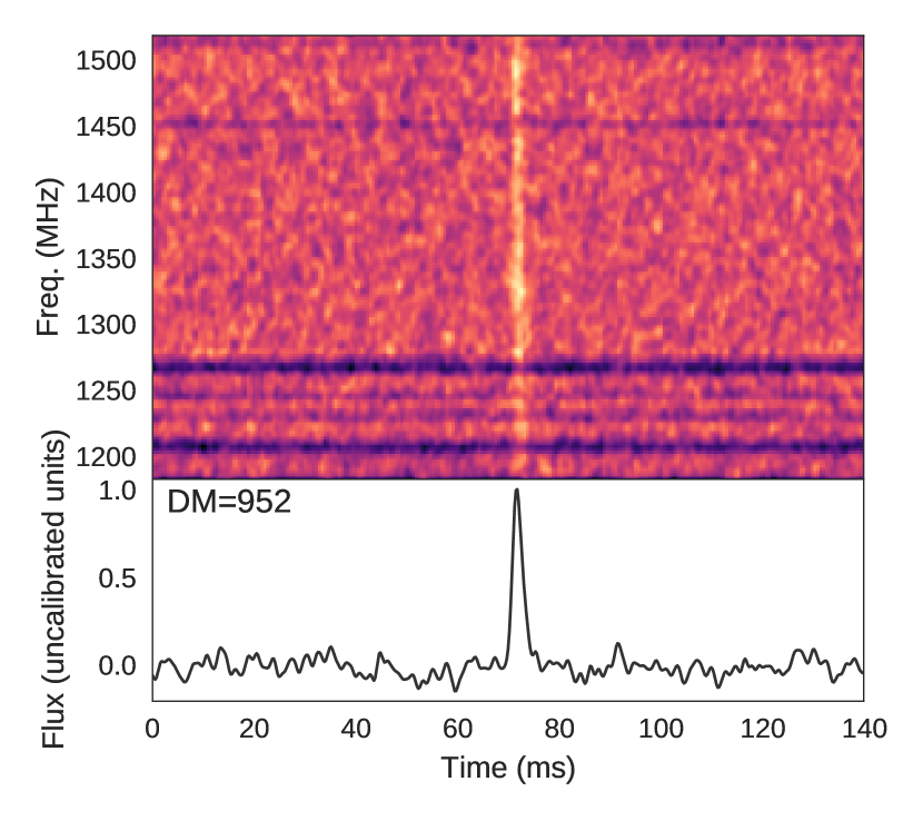
Figure 13: FRB 130626 is a prototypical FRB with a broad-in-frequency, narrow-in-time, single component pulse at a DM of 952 pc cm^-3 which is well in excess of the Galactic DM contribution in that line of sight.

3.1 Data

The one-off nature of FRBs makes it essential to do sufficient due-diligence when reporting on a detection or triggering a follow-up observation to verify a true-positive detection. Over the past decade of FRB surveys, a number of techniques have been developed to efficiently filter the total power, time-frequency data to look for dispersed pulses. Additional and important tests require capturing more data. It is not always possible to capture sufficient data for every desired test, nor is it possible with every observational setup. The effort is, however, justified, as questioning a detection from many possible angles will lead to higher confidence in reporting an event as astrophysical or rejecting it as not interesting.

If most FRBs are indeed one-off events, then the detection data are the only data that will be available. Publication of the detection data allow independent verification, and can be used as input to test independent pipelines. The following should at least be available:

1. A dynamic spectrum which fully encompasses the extent of the dispersed pulse. Preferably, both the raw dynamic spectrum and the RFI flagged and/or normalized spectrum computed in the detection pipeline.

2. Technical data such as time and frequency information, telescope pointing, and other telescope observing parameters.

3. For a multi-beam system, dynamic spectra of each beam covering the extent of the pulse. Similarly for a Tied-Array Beam (TAB) or interferometric detection.

4. The detection parameters such as peak S/N, best DM, pulse width, and others.

5. A list (or guide) of software (including the versions) and parameters used to generate diagnostic plots.

These requirements are typically met in previously reported FRB detections. Often the public data have been normalized and re-quantized to 2 bits for long-term archiving. This reduction in the dynamic range results in potential distortion of pulses, and normalization can hide instrumentational effects. Where possible, the data at the full bit depth, time, and frequency resolution should be stored. The last point, a guide on which software was used is often not reported. Differences in software and data formats can produce different results, such as the reported S/N or time definition. For most of the Parkes detections, filterbank data are publicly available and FRBCAT (Petroff et al., 2016) provides a well-curated repository for information and links to data sources.

To allow for a more complete set of criteria tests and to further improve the evidence of an astrophysical detection, and in addition to the list above, we propose capturing the following:

1. Dynamic spectra which not only encompass the detected pulse, but include data over a longer time spans, e.g. a few minutes before and after the detection. Similarly for multiple feeds, additional TABs, and interferometric baselines.

2. Raw voltage or complex spectral data before power detection and integration that retains time and frequency resolution, and phase information.

A dynamic spectrum extended in time, can be used to find gain and band pass variations. Low-S/N pulse searches can be performed to test if the source repeats or if there is an anomalously high number of events at different DMs. A test observation of a known pulsar nearby in position and time to the detection, perhaps in the beam during the detection, is a useful method to provide a verification of the system state during a detection.

Complex voltages, though costly to capture and store, provide valuable insight. They allow for coherent dedispersion which reduces smearing, and increases the detection sensitivity as in FRB 180301 (Price et al., 2018) where an apparently narrow-band detection was revealed to have low-level flux across a larger band. The time and frequency resolution can be adjusted to look for structure. If multiple sites or elements are used, the signals can be correlated for coincidence detection and localization.

3.2 Criteria

For verification of new FRBs, we propose a list of criteria of two types: the first type tests the similarity between new detections and the prototype, and the second type is used to preclude terrestrial origins of the signal. Together, these two sets provide a framework, which should be used to state the confidence of any new FRB discovery. This list of criteria will improve with time; as new events are discovered, both astrophysical and terrestrial, new tests can be included. The criteria we propose here have been primarily developed from single dish surveys. Use of interferometric arrays will provide powerful further criteria, particularly relevant to localization of signals in the sky.

Included in the criteria are tests to verify whether the telescope was functioning as expected. This is to say that there is a prototypical status for each telescope and receiver system, parametrized by observable quantities, which the data obtained during a detection can be compared against. This comparison requires the availability of the necessary data and expert knowledge of the observer and telescope operators. However, it should be done explicitly when reporting a new detection.

During a search for anomalous signals we expect a number of reported false-positives events, such as Perytons (Burke-Spolaor et al., 2011) and the events presented in Section 2. Public datasets for events that are confirmed as false positives is also extremely useful in defining criteria for classification.

3.2.1 Criteria and scoring suggestions

We define the two types of verification criteria stated above as ‘Similarity to the prototype’ and ‘Terrestrial in origin’. For each criterion, we propose 6 possible answers, which we colour-code in our own categorization below. Answers 1 to 4 are used for the responses: ‘Identical’, ‘Similar’, ‘Not similar’, ‘Completely different’, while 5 and 6 are used for the responses ‘Data not available’ and ‘Test not performed’ respectively.

In the following, we provide a set of questions to help assign a numerical response of 1-6 for each criterion. We have also gone through this process ourselves for a number of published FRBs and other spurious detections, thus providing reference responses for each criterion.

Although it would be tempting to prescribe a combined score, based on which a signal can be classified as an astrophysical FRB or not, the known population is not numerous enough to correctly express all possible true characteristics of the class. At this moment in time, the scores serve, as we demonstrate in the following, to assess individual sources. As the population increases, following this framework of scores should lead to more certain classification. In particular, we have considered carefully the effect of ascribing high scores to values of metrics that fall within the range of verified events. Our reasoning for doing this is that, if a source is scored low for some particular criterion in the following list, but scores highly overall, this only serves in expanding the definition of the prototype. If a source scores low in most criteria, and therefore also overall, it would be hard to objectively classify it as an FRB.

Signal to Noise

What is the measured S/N of the dedispersed, and frequency-collapsed pulse? Can this S/N be verified? The actual S/N could be different from the reported S/N (see Section 2.2). The highest scores should be given for a reliably measured S/N that is both significantly high and within the expected range based on verified FRB detections. Progressively lower scores should be given if the S/N is too low, not verifiable, and/or significantly outside the expected range.

Boresight Flux

What is the implied flux based on the detection S/N and telescope sensitivity, assuming the detection occurred at boresight? Is this within the range of previously reported fluxes? How does it compare to the statistical FRB flux distribution? The majority of reported FRBs have an implied boresight flux between $0.2-2$ Jy, although there is a tail of bright FRBs potentially exceeding 128 Jy (Ravi et al., 2016). Extremely bright FRBs (> kJy) are not expected based on the extensive previous non-detection results from low sensitivity, large sky coverage surveys (Siemion et al., 2012; Karastergiou et al., 2015; Rowlinson et al., 2016). However, extremely bright FRBs can not be completely discounted. The highest score should be given to FRB candidates with fluxes within the range of known sources, and the lowest scores to FRB candidates with the greatest deviation from the known and verified population.

Pulse Width

What is the pulse width of the dedispersed and frequency-collapsed pulse? Is it within the range of previously reported widths? Reported widths range from tens and hundreds of microseconds (FRB 150807, FRB 170827) up to tens of milliseconds (FRB 170922, FRB 160317). The lower pulse width limit is based on the time resolution of the instrumentation, and the pulses may indeed be unresolved. There may be astrophysical FRBs with wider pulse widths, but most historical surveys have had a maximum time-binning scale on the order of tens of milliseconds. FRB 121102 shows a wide range of pulse shapes and widths (Michilli et al., 2018; Gajjar et al., 2017). The highest scores should be given for signals with widths within the range of verified FRB detections.

High-resolution Structure

Search pipelines identify candidates by applying a filter to the dedispersed data. This hides any potential high time and frequency structure that may be present, as in the case of radar signals (Section 2.3). The dynamic spectrum should be checked for sub-structure at both the highest time and frequency resolution. Complex voltages allow for coherent dedispersion and flexibility in channelization and integration, which provides further sensitivity in searching for structure. The highest scores should be given to signals whose high-resolution structure can be explained by a natural process and resembles the structure of verified FRBs. Progressively lower scores should be given as the “distance” from the norm increases.

Multiple components

Are there multiple components to the pulse? And how many? Does this number change when dedispersing with different DMs? Most FRBs appear as single component pulses. But, a few, such as FRB 130729 and some bursts from FRB 121102, show multiple components, which can lead to differences in the ‘optimal’ DM (Michilli et al., 2018). Pulses from FRB 121102 often contain multiple components. As such, it deviates from the prototype. As FRB 121102 is known to be astrophysical, this criterion can not invalidate a detection. If the number of components resembles verified FRBs and other known astrophysical pulses, a high score should be given.

Broad-band

Does the pulse extend in frequency to the edges of the observing band, bottom edge, top edge, both, or neither? A pulse that extends across the full observing band fits the prototypical FRB model. There are now examples of narrow-band (within the observing band) FRBs (such as FRB 121102), as well as narrow-band terrestrial signals, such as radar (Section 2.3), so not having a broad-band signature does not entirely rule out an FRB. We expect this criterion to be improved by future telescope back-ends offering broader bandwidths. Higher scores should be attributed to signals that cover greater extents of the band, in a way that can be explained by a physical process and resembles other verified signals.

Spectral Index

Is there a measurable apparent spectral slope? Deconvolving the instrumental response from the astrophysical spectral response is difficult. Depending on the (mostly unknown) position of a detected pulse within the telescope beam, there will be a frequency-dependent sensitivity response, which will induce chromaticity. If the pulse appears band-limited with a steep spectral index, this could indicate the pulse flux drops below the system noise in parts of the band. If a shallow spectral index is fit to a band-limited pulse, this could indicate the pulse is intrinsically band-limited. Higher scores should be attributed to signals whose spectral slope falls within the range of possible spectral slopes of verified FRBs. Exceedingly steep, in both sense, spectra, should be attributed lower scores.

Scattering

Does the pulse appear to be scattered and/or scintillating? Accurate scattering and scintillation measurements are evidence for radio waves having passed through an inhomogeneous ISM, and can help infer properties of either the host galaxy of the FRB, the media surrounding it, or the IGM.

Scattering timescales are estimated, as in the case of FRB 130626 (Champion et al., 2016), by fitting an exponential tail ($\propto e^{-t/\tau}$, typical of a thin scattering screen) to the scatter-broadened pulse. The characteristic timescale, $\tau$, is expected to have a strong frequency dependence ($\tau\propto\nu^{-\alpha}$), with most models predicting a power law frequency scaling index $\alpha=4$ or $4.4$ (e.g. Rickett 1977), and observations of pulsars often showing $\alpha<4$ (e.g. Lewandowski et al. 2015; Geyer et al. 2017). Spectral indices computed from broad band FRBs, should be compared to these expected values. Measurement of a scattering tail with a spectral index in the range mentioned above warrants the designation of ‘Identical’, while gradual departure from this picture should be described using the other responses.

Comparing obtained $\tau$ values to values predicted by current electron density models for the Milky Way (e.g. Cordes & Lazio 2002; Yao et al. 2017) also provides a test for the extragalactic nature of a detected signal. The closer the scattering characteristics are to what is seen in the verified FRB population, the higher the score should be for this category.

Scintillation

As with scattering, scintillation may also occur due to passage through an inhomogeneous medium. Scintillation in pulsars manifests itself as an organized pattern of time and frequency modulation of the total intensity. For FRBs, the scintillation timescale may be longer than the duration of the pulse, hence not sampled. The scintillation bandwidth on the other hand may be observable due to the broad band systems used for searching. Scintillation bandwidth ($\Delta\nu_{d}$) estimates are obtained by computing the FWHM of the auto-covariance function of the spectrum. The $\Delta\nu_{d}$ measurement corresponds to a broadening (scattering) timescale of $\sim 1/(2\pi\Delta\nu_{d})$.

The highest score should be attributed to sources whose scintillation bandwidth is consistent with a measurement of scatter-broadening, and lower scores for lower consistency. A non-detection of either scattering or scintillation is considered ‘Similar’ (i.e. neutral), until an improved set of categories emerges.

As seen in the XAO event (Section 2.4), frequency modulation can appear similar to scintillation, hence this criterion should be used with care and in conjunction with scattering measurements.

Polarization Characteristics

Were full Stokes parameters measured for the pulse? Does the pulse show polarization characteristics? Can a rotation measure be fit to the pulse? Positive answers to these questions should result in a high score. Multiple FRBs have been reported to be polarized (Petroff et al., 2015a; Masui et al., 2015; Keane et al., 2016; Ravi et al., 2016; Petroff et al., 2017b; Caleb et al., 2018). For example, FRB 121102, appears to be linearly polarized after the extreme Rotation Measure (RM) is corrected for (Michilli et al., 2018), and FRB 110523 is measured to have a high fraction ($\sim$ 44%) of linear polarization. Where possible, it is insightful to compare RM values to RM measurements of nearby pulsars. The RM estimate for FRB 110523 was compared to an observation of PSR B2319+60, within 2 degrees on the sky, using the same pipeline. RFI has complex polarization characteristics, such as Phase-shift keying (Horowitz & Hill (2015), Chapter 13), as a way of encoding information. These encoding schemes will appear different from polarized astrophysical sources, and will not be well fit by a Faraday rotation model. Low scores should be attributed to candidates with artificial polarization characteristics, and higher scores to candidates where the polarization can be understood by the aforementioned physical processes.

DM Excess

What is the S/N-maximized DM? How does this compare to the modeled Galactic DM along the line of sight? Is it well in excess of the Galactic contribution? This is a standard test to differentiate between a Galactic and extragalactic source. If the ratio of measured DM to Galactic model DM is at least a factor of two then the source is likely extragalactic. Otherwise the source is likely a pulsar or RRAT within the Galaxy. If there are multiple components, what is the ‘component-optimized’ DM, how does it differ from the S/N-maximized DM? When there are multiple components to a pulse, the choice of DM can result in different frequency-averaged pulses such as in FRB 130729 in which the choice of DM can result in a single component or multi-component pulse profile (see Section 4.1). Lower scores should be attributed to candidates whose DM could be explained as Galactic.

3.2.2 Terrestrial Origins

Dispersion Relation

Does the pulse follow a cold plasma $\nu^{-2}$ dispersion relation? If there is sufficient S/N in individual time-frequency bins across a significant fractional bandwidth of the dynamic spectrum then a dispersion relation fit showing a $\nu^{-2}$ relation is evidence for a dispersed, natural source. Conversely, a fit that diverges from $\nu^{-2}$ is good evidence for an artificial source (Section 2.4). Performing model selection between a $\nu^{-2}$ relation model and other models can be done to statistically compare models.

DM Trial Space

In a DM trial space search (positive and negative DM trials) are there other high-S/N events nearby in time to the detected pulse? If there are few other events above during the time window then that is evidence for a true detection. But, if there are events seen at similar S/N, especially in the negative DM space, then it could be that the RFI environment has increased the false-positive event rate.

Repeating Events

Repeating events are evidence for either an astrophysical or a terrestrial origin. Most FRBs appear to be one-off events, but if the source does repeat then it can be localized or verified with another telescope. If the source repeats at different points such as the XAO event, then the source is terrestrial.

Were follow-up observations performed to search for repeating events? Was a lower-S/N search performed around the detected DM in the survey data? If the source does repeat, what was the time scale? Could a periodicity search be performed? And, did the repeating events occur at different telescope pointings?

The current prototype is considered to be a once-off burst. We label the repeating FRB 121102 as ‘Not Similar’ to the prototype. Further detection of repeating FRBs will facilitate changing the prototype model.

RFI Environment

An excess in RFI during a detection compared to the typical RFI environment reduces the confidence in an astrophysical detection. Was the RFI environment drastically different during the event detection compared to typical observations? What was the effective bandwidth of the receiver after RFI flagging? If the RFI environment was different, there could be an increase in the number of false-positive events, likely seen in the DM trial space test. Or, the reduced bandwidth can limit a $\nu^{-2}$ dispersion relation fit.

Telescope State

While on the surface a trivial criterion, it is important to check that the telescope was in a valid state. For example, was the analog signal chain in a linear state, was the feed in the correct position, was other equipment active that could cause local interference? This is a site and telescope-dependent criterion, which requires expert knowledge of the system in order to test this criterion with due diligence. A regular test of the overall telescope state would be to observe a known pulsar during observations.

Bandpass Variation

During the event, does the bandpass shape appear similar to the expected bandpass seen in typical observations? Most search pipelines apply a bandpass correction to normalize the noise variance. This flattens the bandpass, and hides any changes in the measured bandpass response. The first indication that the electronics were not functioning correctly in the ALFABURST event (Section 2.1) was the change in bandpass response.

Gain Stability

Does the gain show similar variance over a window of time around the event compared to the gain variation seen in typical observations? Similar to bandpass normalization, a high-pass filter is often applied in a search pipeline to reduce long-term gain variations. This may be hiding differences in gain variation during an event detection. The gain stability of a system during an event detection should be similar to the stability on a longer time scale around the detection.

Telescope Pointing

Where was the telescope pointing in the local reference frame? Was it near the horizon or known RFI sources? Weak RFI sources on the horizon are picked up by the high forward gain of dish telescopes. And, strong RFI sources can still be picked up in the side and back-lobes of the beam, or directly illuminate the feed.

Were there known satellites in the primary or side-lobes of the beam? For example, geosynchronous satellites are located within $\pm 15^{\circ}$ declination (Anderson et al., 2015). Publicly available satellite orbital parameters can be used to determine the presence of a satellite near a telescope pointing position. The transponder frequencies and positions of commercial satellites are regularly maintained, though not all are publicly reported, e.g. military satellites. The presence of a satellite operating at frequencies in the observing band will result in an increase in the overall system gain. But, if the gain has been normalized the source might not be apparent.

Local Time

What was the local time of the detection? Was there regularly scheduled maintenance? Does the time coincide with an increase in local RFI, as in the case of Perytons (Section 2.5)? Or, for a commensal system, what was the primary observing schedule? It could be that equipment was active which typically is not during standard observations, such as the ALFA candidate (Section 2.1).

Multi-beam

Is the receiver a multi-beam system? Was the pulse detected in multiple beams? If so, is there a difference in S/N between beams? Multi-beam systems, in particular the Parkes multi-beam receiver, have been very successful in the detection of FRBs as they provide good evidence for an event occurring in the far-field versus in the near-field. A multi-beam system can be used to perform coincidence detection to significantly reduce the number of false-positive detections. FRB 010724 (Lorimer et al., 2007) was detected in multiple beams of the Parkes multi-beam receiver, but at different sensitivities indicating that the source, though extremely bright, was localized to a position in the sky. Perytons were also detected with the Parkes multi-beam receiver but in all beams at similar sensitivities indicating the source was local (Burke-Spolaor et al., 2011).

Tied-array Beam (TAB)

Was the pulse detected with a TAB using an array of elements? If so, was the pulse seen in individual elements? Were multiple TABs active during the observation? If so, was the pulse seen in multiple beams? Similar to a multi-beam detection, a tied-array beam detection can be used to determine if the source was in the near-field. Further, the near-field limit of a tied array is typically much larger than that of a dish. For example, the near-field limit of Parkes is $\sim 40$ km, while Farah et al. (2018) set a near-field limit of the source of FRB 170827 to $\geq 10^{4}$ km with a tied-array detection which can rule out the source being local up to medium Earth orbits. If the individual element data are available, then subsets of elements can be combined to show the source was detected in most elements rather than just in one or a few.

Interferometric Array

Was the pulse detected while baseline correlations were recorded in an interferometric mode? Was the pulse localized within the primary beam? Is the pulse detected on individual baselines? Similar to the tied-array criterion, an interferometric detection can determine if the source was in the near field. An FRB detection on baselines $\geq 10$ km at L-band frequencies would be sufficient to determine if the source is a terrestrial satellite. Interferometric detection of a pulse provides strong evidence by removing element auto-correlation effects. Though, local RFI will persist, synthesis imaging can be used to localize the source.

Multi-site Observations

Was the pulse detected in a multi-site observation campaign? If so, was the pulse detected at multiple sites? Multi-site detection is very strong evidence for a pulse being astrophysical.

4 Application of FRB criteria to previous detections

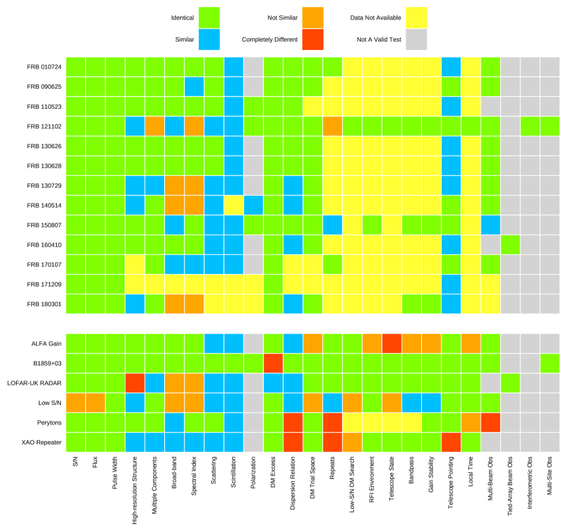
Figure 14: Verification criteria (Section 3.2) heat map of some of the previously reported FRBs (top) and the terrestrial sources discussed in this work (bottom). Green indicates a criterion test is identical to the prototypical detection or observation, thus providing evidence in favour of an astrophysical origin. Blue indicates a criterion test result is similar to the prototype, but is not identical, and thus, is neutral evidence of an astrophysical origin. Orange indicates the criterion results deviates from the expected prototype result and the event may be of terrestrial origin. Red indicates the criterion result is completely different from the prototype, and the event is terrestrial in origin. Yellow indicates the criterion result could not be determined from the available data. Grey indicates the criteria is not valid based on the observation.

4.1 FRB signals

Having provided the FRB verification criteria above, we have re-analyzed the previous reported FRBs based on the available literature and public data. This analysis provides examples of answers 1-6 from Section 3.2 for a number of sources. Figure 14 captures the results in a colour-coded table. Overall, it is clear that the detections reported in the literature score well against the prescribed criteria, which is to be expected as many of these criteria are implicit to the observational definition of an FRB such as high S/N and a line of sight dispersion measure in excess of the Galactic contribution.

Starting from the lowest scores in our sampled set, we note that FRB 130729 is band-limited to the lower half of the observing band, and there is a sharp decrease in flux around 1350 MHz (Figure 15). We are using a dispersion measure of 852 pc cm^-3 which is different from the originally reported dispersion measure of 861 pc cm^-3. Using this new dispersion measure there are two distinct components. The original detection paper (Champion et al., 2016) notes that FRB 130729 is potentially due to terrestrial RFI, which is made clear in the low criteria scores.

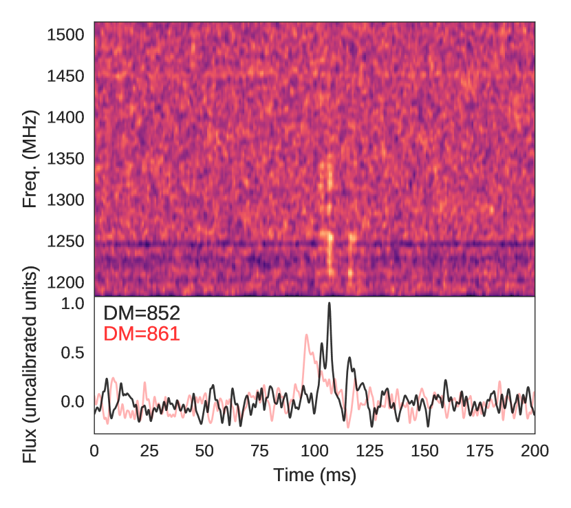
Figure 15: FRB 130729 dedispersed with a DM of 852 pc cm^-3 (black), this is different from the DM of 861 pc cm^-3 (red) reported in Champion et al. (2016). The detected FRB has two distinct components separated by approximately 10 ms. Data are presented at the native recorded resolution of 64 $\mu$s, 390 kHz convolved with a Gaussian smoothing filter of size 512 $\mu$s, 3.125 MHz.

FRB 140514 (Figure 16) and FRB 180301 (Figure 17) both score poorly in the broad-band criteria as the majority of the detected flux is concentrated into narrow regions of the band. This low score affects the dispersion relation criteria test as there is not sufficient fractional bandwidth to perform a good fit. The frequency structure of both of these detections could be due to scintillation or plasma lensing. These low scores do not discount FRB 140514 and FRB 180301 as astrophysical, they indicate that FRB 140514 and FRB 180301 diverge from the prototypical FRB model. We note that FRB 121102 diverges significantly from the prototype model as individual pulses vary in bandwidth, apparent scattering, spectral index, and structure. This is a useful example to show that the highest test scores are not needed to verify a detection as astrophysical.

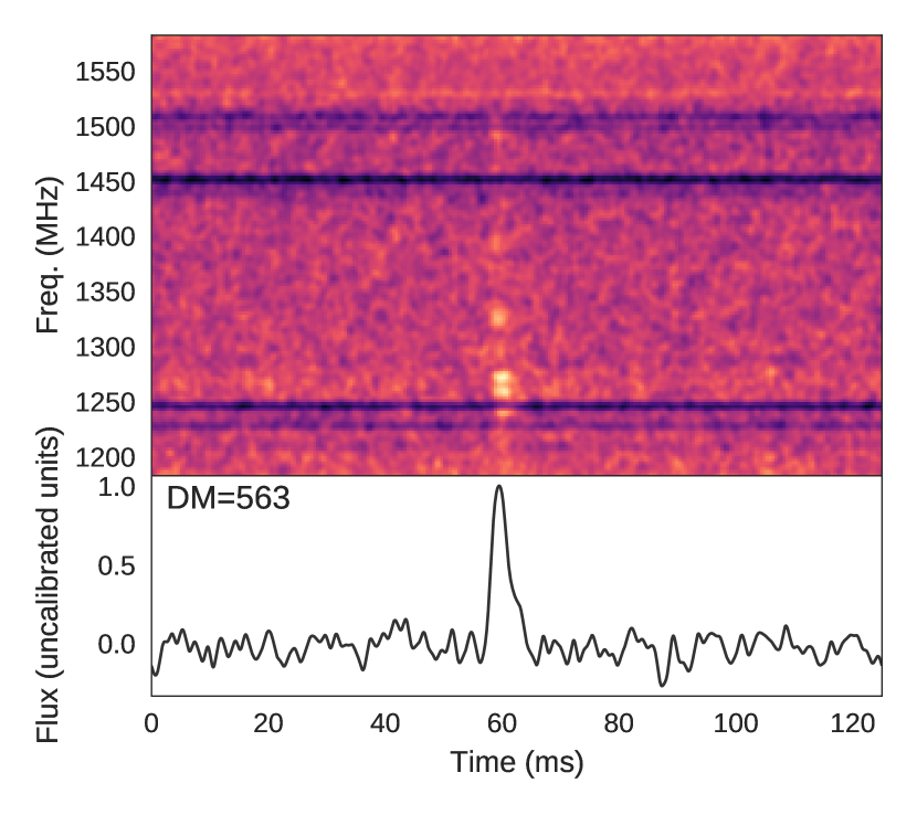
Figure 16: Dynamic spectrum of FRB 140514 dedispersed with a DM of 563 pc cm^-3. Data are presented at the native recorded resolution of 64 $\mu$s, 390 kHz convolved with a Gaussian smoothing filter of size 512 $\mu$s, 3.125 MHz.

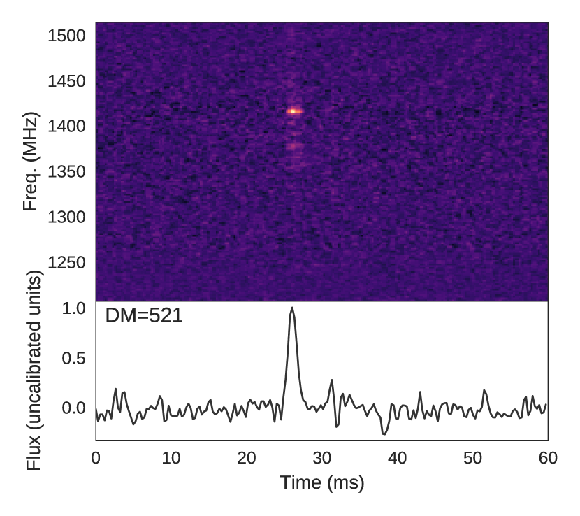
Figure 17: Dynamic spectrum of FRB 180301 dedispersed with a DM of 521 pc cm^-3. data are presented at the native recorded resolution of 292.57 $\mu$s, 437.5 kHz convolved with a Gaussian smoothing filter of size 29.2 $\mu$s, 875 kHz.

FRB 010724 (Lorimer et al., 2007), being the first reported detection, fits the prototypical model well as many of the standard criteria we now use were initially decided in the detection report. Similarly, FRB 110523, FRB 130626, and FRB 130628 all match the prototypical model well, and thus show high scores in most of the tests. FRB 090625 shows variation in flux across the band, possibly due to beam colorization or scintillation. This is indicated by the lower spectral index criteria score, but FRB 090625 is otherwise also prototypical. FRB 150807 shows a drop in flux at the high end of the observing band due to a steep apparent spectral index which is either intrinsic to the source or due to the beam response. The reported detection included a number of system state tests such as checking the gain and bandpass response, and the RFI environment which increases the overall score of this detection.

In most cases, detections do not report on the telescope state and environment during the time of detection. Though data are made public in many of the detections, these data have already been normalized or calibrated so it is not possible to verify the telescope state. More recent detections are often lacking in data or detailed analysis. For example, very little information on FRB 171209 has been reported, thus almost none of the criteria can be tested. Providing public data not only allows for independent verification, but also for new tests on previous detections. For example, the lack of public data of FRB 170107 means that criteria not reported in the initial detection can not be tested.

4.2 Terrestrial signals

Also included in Figure 14 are the results for the various detections discussed in Section 2. We also include PSR B1859+03 as an example of single pulses from a pulsar during the ALFABURST surveys. In all these cases there is at least one failure. The LOFAR radar event shows artificial high-resolution structure. Perytons and the XAO repeater fail the dispersion relation test and repeat at different telescope pointings. The ALFA gain variation has multiple negative test results relating to the system response compared to the expected response. The low S/N event does not have a single critical test failure but fares poorly in several tests. No single test is sufficient to decide that an event is terrestrial. Figure 14 demonstrates how, given enough tests, a strong case can be made to classify all these events as terrestrial.

5 Future Observational Methods

Beyond detection of more FRBs, the goals of current surveys are to localize the source to host galaxies, and detect pulses across broader bandwidths and different frequencies in the radio spectrum. Verifiability should also be considered in these surveys. This means capturing additional data as discussed in Section 3.1 and additional observing methods.

The simultaneous detection of a signal with telescopes at multiple sites is clear evidence for an astrophysical FRB. Multi-site detectors, such as the Laser Interferometer Gravitational-Wave Observatory (LIGO), are essential for false-positive rejection. Coordinated telescope observations is logistically difficult but would prove invaluable in reporting detections. Telescopes do not need to be observing at the same frequency, only observing the same approximate field of view. Detection of an event at multiple bands is strong evidence for an astrophysical source. Though, multi-frequency observation campaigns of FRB 121101 have shown that detections can be band-limited (Law et al., 2017).

Localization with an interferometric array produces similar results to a multi-site observation. RFI local to the site will still appear but it can be better localized, and possibly determined to be in the near field. RFI internal to a single element would not correlate with other elements and would not appear as a false-positive detection. Very-Long Baseline Interferometry (VLBI) detections provide the highest confidence as the source is localized with multiple geographically isolated telescopes.

Detection of FRBs at multiple frequencies not only adds to the scientific understanding of the sources, but also helps to verify that they are astrophysical. Due to historical development of receivers for pulsar searches, most FRBs have been detected at L-band frequencies. FRB 110523 detected with the GBT and the multiple FRBs detected with UTMOST occurred at UHF frequencies. Only FRB 121102 has been detected above L-band (Law et al., 2017; Gajjar et al., 2017; Michilli et al., 2018; Spitler et al., 2018). Such wide bands show the pulse structure goes beyond the bandwidth of known sources of RFI (e.g. modulated radar).

Multiple FRBs (e.g. FRB 121102, FRB 140514, FRB 180301) have now been detected which are not broad-band, possibly due to the intrinsic emission of the source, lensing, or scintillation. It is likely that additional narrow-band FRBs exist in past survey data but do not pass the detection threshold. A pulse search over sub-bands could reveal further detections as the S/N would increase.

An ideal FRB search experiment would consist of at least three stations geographically separated to reduce common RFI and allow for localization. Each station would consist of an aperture array or a compact array of small-diameter/wide field of view elements. The effective bandwidth would be sufficient to accurately determine a dispersion relation. Coherent beams would be formed across the primary beam. Each station would observe the same field. Detections at multiple sites would then trigger a capture of the complex voltages in a transient buffer which could then be correlated after the fact.

Though this idealized experiment does not exist, it is currently possible to make experiments that are close to it. LOFAR stations, though very low-frequency compared to previous detections, can be configured to operate in a similar mode. Dense arrays such as UTMOST (Caleb et al., 2017), which has detected numerous FRBs, and CHIME (The CHIME/FRB Collaboration et al., 2018) provide significant instantaneous sky coverage but limited spatial resolution. The planned build-out of the Molonglo array to UTMOST-2D will provide further localization. Additional outrigger elements such as those planned with HERA (DeBoer et al., 2017) would provide an improvement in spatial resolution. TRAPUM, one of the MeerKAT legacy science projects, and MeerTRAP, a commensal transient search program on MeerKAT, will perform single pulse surveys in beamformed data and capture complex voltage data for post-detection localization. Telescopes that are part of VLBI networks use the same back-ends and contain complex voltage recorders, can be used (Walker et al., 2018). Only a few telescopes in the network that can have the same pointing are needed at a time for localization.

6 Conclusion

From an observational point of view, FRBs are unique astronomical sources as, so far, no follow-up observations have been able to verify a source using a different telescope or observing frequency, except in the case of FRB 121102 which is known to repeat. Thus, it is necessary to provide evidence for an astrophysical origin when reporting a detection.

In Section 3 we have presented a set of criteria which can be used to verify an FRB detection relative to a prototypical FRB model and observational data. We have shown which of the criteria are more essential to verification than others. For example, the strongest evidence for an event being of astrophysical origin is a multi-site detection. In combination these criteria become stronger evidence for the origin of a detected FRB. Effort should be made to test these criteria using the available data when reporting a detection. The set of criteria and methods for applying them laid out here should ideally be applied to all new FRB detections. Publishing a table similar to Figure 14 provides comprehensive information for assessing new detections.

As FRB surveys continue to increase in sensitivity, sampled parameter space, and time, there will be an increase in the number of false-positive detections, even as rejection models are improved. Differentiating between true, astrophysical FRBs and false-positive events will become more difficult. Further, it could be that most astrophysical FRBs are not prototypical as it is defined now, such as in the case of FRB 121102. Which indicate that some of the criteria must be relaxed, making the differentiation more difficult still. This should warrant the drive towards interferometric and multi-site observations, complex-voltage data recorders, sub-band pulse searches, and standard reporting of the observing system.

Automation of some of the verification tests can help to formalize criteria into metrics. Machine learning-based models are routinely employed to detect and classify candidate detections. Zhang et al. (2018) used simulated pulses to train a deep neural network detection model. Connor & van Leeuwen (2018) built a classifier model based on the dynamic spectrum, pulse profile, and DM-trial space of a detection. This model was similarly trained with simulated pulses. UTMOST FRB detections (Farah et al., 2018) are automated through the use of a classifier model which takes into account multi-beam detections to reduce the number of false-positive detections due to local RFI. The ALFABURST system (Foster et al., 2018) which detected the event in Section 2.1 uses a similar classifier model. Inherent to these models is a definition of a prototype pulse. They provide the initial assessment of the detection, which can then be followed by testing the more complex criteria which still require expert analysis.

Detection reporting incurs an economic cost in observing time, resources, and human effort. Though, there is a scientific cost to delayed reporting as follow-up observations could detect further pulses or multi-wavelength observations could reveal an unknown counterpart to the radio pulse. An initial detection will not be able to be verified against many of the criteria presented here. But basic tests such as S/N, dispersion relation, and telescope state can be automated to determine an initial detection ‘importance’ in a VO-Event trigger (Petroff et al., 2017a). This importance factor can then be adjusted accordingly as more criteria are tested.

Reporting of false-positive events, even if the source is not explained, helps to improve the robustness of search pipelines against systematics and RFI. Reporting these events also helps to improve the case for FRBs being of astrophysical origin, just as the explanation for Perytons (Petroff et al., 2015b) removed doubt about detections using Parkes. An attempt should be made to make the raw data, either unprocessed filterbank or complex-voltage data, available to be used in independent verification and testing on search pipelines.

Jupyter notebooks of the verification tests and terrestrial FRBs are hosted on our public git repository.

References

- Anderson et al. (2015) Anderson P. V., McKnight D. S., Pentino F., Schaub H., 2015, in 66th International Astronautical Congress, IAC-15 A. p. 7
- Bannister et al. (2017) Bannister K. W., et al., 2017, ApJ, 841
- Barsdell et al. (2012) Barsdell B. R., Bailes M., Barnes D. G., Fluke C. J., 2012, MNRAS, 422, 379
- Burke-Spolaor et al. (2011) Burke-Spolaor S., Bailes M., Ekers R., Macquart J.-P., Crawford III F., 2011, ApJ, 727, 18
- Caleb et al. (2017) Caleb M., et al., 2017, MNRAS, 468, 3746
- Caleb et al. (2018) Caleb M., et al., 2018, MNRAS, 478, 2046
- Champion et al. (2016) Champion D. J., et al., 2016, MNRAS, 460, L30
- Chennamangalam et al. (2017) Chennamangalam J., et al., 2017, ApJS, 228, 21
- Connor & van Leeuwen (2018) Connor L., van Leeuwen J., 2018, preprint, (arXiv:1803.03084)
- Cordes & Lazio (2002) Cordes J. M., Lazio T. J. W., 2002, ArXiv/0207156,
- Cordes et al. (2017) Cordes J. M., Wasserman I., Hessels J. W. T., Lazio T. J. W., Chatterjee S., Wharton R. S., 2017, ApJ, 842, 35
- DeBoer et al. (2017) DeBoer D. R., et al., 2017, PASP, 129, 045001
- Eatough et al. (2009) Eatough R. P., Keane E. F., Lyne A. G., 2009, MNRAS, 395, 410
- Farah et al. (2018) Farah W., et al., 2018, MNRAS, 478, 1209
- Foster et al. (2018) Foster G., et al., 2018, MNRAS, 474, 3847
- Gajjar et al. (2017) Gajjar V., et al., 2017, FRB 121102: Detection at 4 - 8 GHz band with Breakthrough Listen backend at Green Bank, ATel 10675
- Geyer et al. (2017) Geyer M., Karastergiou A., Kondratiev V. I., Zagkouris K., Kramer M., Stappers B. W., et al. 2017, MNRAS, 470, 2659
- Horowitz & Hill (2015) Horowitz P., Hill W., 2015, The Art of Electronics. Cambridge University Press
- Karastergiou et al. (2015) Karastergiou A., et al., 2015, MNRAS, 452, 1254
- Keane et al. (2016) Keane E. F., et al., 2016, Nature, 530, 453
- Law et al. (2017) Law C. J., et al., 2017, The Astrophysical Journal, 850, 76
- Lewandowski et al. (2015) Lewandowski W., Kowalińska M., Kijak J., 2015, MNRAS, 449, 1570 (L15)
- Lorimer et al. (2007) Lorimer D. R., Bailes M., McLaughlin M. A., Narkevic D. J., Crawford F., 2007, Science, 318, 777
- Masui et al. (2015) Masui K., et al., 2015, Nature, 528, 523
- Michilli et al. (2018) Michilli D., et al., 2018, Nature, 553, 182
- Ofcom (2017) Ofcom 2017, Technical Report 18, United Kingdom Frequency Allocation Table. Ofcom
- Oostrum et al. (2017) Oostrum L. C., et al., 2017, Detection of a bright burst from FRB 121102 with Apertif at the Westerbork Synthesis Radio Telescope, ATel 10693
- Petroff et al. (2015a) Petroff E., et al., 2015a, MNRAS, 447, 246
- Petroff et al. (2015b) Petroff E., et al., 2015b, MNRAS, 451, 3933
- Petroff et al. (2016) Petroff E., et al., 2016, Publ. Astron. Soc. Australia, 33, e045
- Petroff et al. (2017a) Petroff E., et al., 2017a, preprint, (arXiv:1710.08155)
- Petroff et al. (2017b) Petroff E., et al., 2017b, MNRAS, 469, 4465
- Price et al. (2018) Price D. C., et al., 2018, Detection of a new fast radio burst during Breakthrough Listen observations, ATel 11376
- Ravi et al. (2016) Ravi V., et al., 2016, Science, 354, 1249
- Rickett (1977) Rickett B. J., 1977, ARA&A, 15, 479
- Rosch et al. (1976) Rosch E., Mervis C. B., Gray W. D., Johnson D. M., Boyes-Braem P., 1976, Cognitive Psychology, 8, 382
- Rowlinson et al. (2016) Rowlinson A., et al., 2016, MNRAS, 458, 3506
- Siemion et al. (2012) Siemion A. P. V., et al., 2012, ApJ, 744, 109
- Spitler et al. (2016) Spitler L. G., et al., 2016, Nature, 531, 202
- Spitler et al. (2018) Spitler L. G., et al., 2018, The Astrophysical Journal, 863, 150
- The CHIME/FRB Collaboration et al. (2018) The CHIME/FRB Collaboration et al., 2018, preprint, (arXiv:1803.11235)
- Thornton et al. (2013) Thornton D., et al., 2013, Science, 341, 53
- Wagstaff et al. (2016) Wagstaff K. L., et al., 2016, PASP, 128, 084503
- Walker et al. (2018) Walker C. R. H., et al., 2018, preprint, (arXiv:1804.01904)
- Yao et al. (2017) Yao J. M., Manchester R. N., Wang N., 2017, ApJ, 835, 29
- Zhang et al. (2018) Zhang Y. G., Gajjar V., Foster G., Siemion A., Cordes J., Law C., Wang Y., 2018, The Astrophysical Journal