Reweighting a parton shower using a neural network: the final-state case

Abstract

The use of QCD calculations that include the resummation of soft-collinear logarithms via parton-shower algorithms is currently not possible in PDF fits due to the high computational cost of evaluating observables for each variation of the PDFs. Unfortunately the interpolation methods that are otherwise applied to overcome this issue are not readily generalised to all-order parton-shower contributions. Instead, we propose an approximation based on training a neural network to predict the effect of varying the input parameters of a parton shower on the cross section in a given observable bin, interpolating between the variations of a training data set. This first publication focuses on providing a proof-of-principle for the method, by varying the shower dependence on $\alpha_{\text{S}}$ for both a simplified shower model and a complete shower implementation for three different observables, the leading emission scale, the number of emissions and the Thrust event shape. The extension to the PDF dependence of the initial-state shower evolution that is needed for the application to PDF fits is left to a forthcoming publication.

1 Introduction

With the Large Hadron Collider (LHC) successfully undergoing its second run and the possible upgrade to the so-called High-Luminosity LHC, the produced collision datasets reach new levels of precision. This requires an ongoing effort to provide more precise theory predictions. A sizeable part of the overall theory uncertainty is often given by the degree to which we know the parton content of the incoming protons, parametrised by the parton density functions (PDF) [1, 2, 3, 4], see also Ref. [5] and references therein for a recent review. In order to increase the precision of PDF determinations, it is clearly desirable to be able to include as many observables as possible in the fits. However the $\chi^{2}$ minimization in these fits needs multiple re-evaluations of the underlying observables in order to converge. As a result there are strict constraints on the CPU time each re-evaluation costs: observables can be included in fits only if there is an efficient way to compute them as PDFs are varied. For instance, in nnpdf fits, all observables are written as convolutions of FK tables and PDFs at the initial scale as discussed in detail in Ref. [6]. Similarly, some results provided by Monte-Carlo event generators, e.g. NLOJet++ [7], MadGraph5_aMC@NLO [8], mcfm [9] or sherpa [10], can be projected onto an interpolation grid, which allows fast a-posteriori variations of the input parameters, because the sum over simulated events is replaced by a sum over a much smaller number of observable-dependent weights [11, 12, 13, 14, 15, 16]. Unfortunately, as explained later in this work, this approach cannot be easily extended to capture the input-parameter dependences of the all-order predictions obtained by the parton-shower algorithms in Monte-Carlo generators.

Instead we present here an approximate approach to parametrise the parton-shower dependences in a way that allows for a fast, a-posteriori reweighting of the observable. Because we are dealing with binned observables, the output of the parton shower is the number of events in a given bin. In this context ’reweighting the observable’ means finding the relative weight of each bin as the input parameters change, i.e. recomputing the value of the observable in each bin. Once the relative weight is known, the number of events in a bin can be easily recomputed by multiplying its original value by the new weight. A quick summary of the method is as follows. First, the calculation is repeated for a given set of input parameters. The variation of the result (in a given observable bin) across this set is then used to train a neural network (NN), effectively fitting the unknown functional form that encodes the dependences of the parton shower on the input parameters. This NN can then be used to obtain efficiently an interpolation of the observable for arbitrary values of the input parameters, so that it is suitable to use this methodology in studies that require fast a-posteriori variations.

NN techniques have been successfully applied or used exploratively in a number of topics in collider phenomenology, often with much more complex NN architectures than what we employ in this work. The topics include jet tagging/particle identification [17, 18, 19, 20, 21, 22, 23, 24, 25], event classification [26, 27, 28], phase-space integration [29], pile-up mitigation [30], simulating electromagnetic showers in a calorimeter [31], parameter space scans for New Physics searches [32], and of course PDF fitting [1]. Moreover, a deep NN has been proposed to mimic a parton shower algorithm [33]. However, this latter ansatz can not be applied to our goal of using all-order results in PDF fits, as it is applied on an event-by-event basis just as an ordinary parton-shower algorithm, whereas PDF fits require projections of the cross section on observables in order to achieve the fast evaluation times needed for the fit. The interplay of parton showers and NN has also been studied in [34], in which the authors investigate the role of parton-shower uncertainties and approximations in NN-based jet substructure analyses. In [35] an NN is used to determine the effective correction to a Sudakov form factor in a minlo calculation of single-top plus jet production.

In this exploratory study, we restrict ourselves for simplicity to final-state parton showers. While these are not dependent on PDFs, the problems that need to be addressed are the same that would appear in a PDF fit. This simplified setting allows us to test our ideas without getting bogged down in technicalities. The same approach can be readily generalised to include PDF-dependent initial-state emissions. In the latter case, having to deal with a much larger space of parameters entails a number of algorithmic issues that will be addressed in future studies.

In Sec. 2, we summarise the main steps in the algorithm for reweighting a parton shower on-the-fly, highlighting the fact that a straightforward generalisation of the interpolation approach used e.g. in Ref. [14] does not seem feasible. Understanding the limitations of that approach is particularly useful in order to motivate our choices on how to set up and train neural networks to reproduce this reweighting. We formulate our NN-based approach in Sec. 3 and describe the toy parton-shower implementation used for validating the approach. The validation method and its results are presented in Sec. 4. The approach is then further tested in Sec. 5 with a full shower implementation given by the default sherpa parton shower for the prediction of the Thrust event shape at a lepton-lepton collider. Finally, we give our conclusions in Sec. 6.

2 Reweighting the Sudakov Veto Algorithm

2.1 On-the-fly reweighting of parton-shower emissions

Parton-shower algorithms generate exclusive parton emissions starting from a simulated event of a given high-energy process. They are based on a re-formulation of the dglap evolution [36, 37, 38] using Sudakov form factors $\Delta$ with an emission kernel $K$ [39]. The Sudakov form factor gives the probability that no (resolvable) emission occur between two emission scales $t_{\text{low}}<t_{\text{high}}$:

$$\Delta(t_{\text{high}},t_{\text{low}})=\exp\left(-\int_{t_{\text{low}}}^{t_{\text{high}}}\text{d}t\,K(t)\right)\,.$$ (1)

We will further specify $t$ and $K$ when we describe our simplified shower model in Sec. 3.1. For now, we only need to know how parton-shower algorithms numerically generate emissions between $t_{0}$, the starting scale of the shower usually given by a characteristic scale of the high-energy event simulated in fixed-order perturbation theory, and $t_{\text{IR}}$, the infra-red cut-off scale of the parton shower, where the evolution would be typically handed over to a fragmentation algorithm to hadronise the low-energy partons.

The first step is to find the splitting scale $t$ for the next emission. To achieve this, a random number could be used to sample the kernel $K(t)$ of Eq. (1). However, doing this in a direct way requires $K$ to be integrable and invertible. This is not the case for most parton-shower kernels. A way around this is the Sudakov Veto Algorithm [40, 41, 42, 43, 44, 45]. Herein, one replaces $K$ with a new kernel $\hat{K}$, for which we know the integral $\hat{\mathcal{K}}$ and its inverse, and which satisfies $\hat{K}(t)\geq K(t)$ for all $t$. The algorithm then goes as follows:

1. Set $t\to t_{0}$, stop if $t_{0}<t_{\text{IR}}$.

2. Set $t\to\hat{\mathcal{K}}^{-1}(\log(R_{1})+\hat{\mathcal{K}}(t))$ with a random number $R_{1}$, stop if $t<t_{\text{IR}}$.

3. Set $P_{\text{acc}}\to K(t)/\hat{K}(t)$. If $P_{\text{acc}}>R_{2}$ for a new random number $R_{2}$, the emission is accepted.

4. Return to Step 2.

The hit-or-miss Step 3 counter-balances sampling the “wrong” kernel $\hat{K}$ in Step 2. When the algorithm stops, we have a list of scales $t^{\text{acc}}_{i}$ for the generated (i.e. accepted) emissions and a list of scales $t^{\text{rej}}_{i}$ for the rejected emissions. We can call this the parton-shower history of the event in terms of $t$.

Let us ask the following question now: if we have a given shower history generated according to a kernel $K$, what are the relative probabilities

$$w_{k}=\frac{P(\{t^{\text{acc}}_{i}\},\{t^{\text{rej}}_{i}\}|K_{k})}{P(\{t^{\text{acc}}_{i}\},\{t^{\text{rej}}_{i}\}|K)}$$

to generate the same histories for a set of alternate kernels $K_{k}$? It turns out that these probabilities are given by [45]

$$w_{k}=\prod_{i}q^{k}_{\text{acc}}(t^{\text{acc}}_{i})\cdot\prod_{j}q^{k}_{\text{rej}}(t^{\text{rej}}_{j})\,,$$ (2)

where we have defined the reweighting factors

$$q^{k}_{\text{acc}}(t) =\frac{K_{k}(t)}{K(t)}\,,$$

$$q^{k}_{\text{rej}}(t) =\frac{\hat{K}(t)-K_{k}(t)}{\hat{K}(t)-K(t)}=1+(1-q_{\text{acc}}^{k}(t))\frac{P_{\text{acc}}(t)}{1-P_{\text{acc}}(t)}\,.$$

The acceptance probability $P_{\text{acc}}$ in the second form given for $q^{k}_{\text{rej}}$ is defined as in Step 3 in the Sudakov Veto Algorithm.

In an event generation, storing the relative probabilities $w_{k}$ then allows to reconstruct the spread of an observable under the variations labelled by $k$ in a more efficient way than if we would do separate re-runs of the simulation for each $K_{k}$. This parton-shower reweighting is implemented in the three most commonly used parton-shower implementations [46, 47, 48]. It complements reweighting strategies for fixed-order calculations and allows a comprehensive reweighting of the perturbative parts of an event generation when the interplay between matrix elements and parton showering is properly accounted for in the reweighting [48].

2.2 The troubles with exact a-posteriori approaches

The applicability of the parton-shower reweighting described in the previous section is restricted to cases, where the required variations are known beforehand. In principle one could store all parton-shower history data needed to perform reweightings a-posteriori, but as each history will typically have $\mathcal{O}(10)$ accepted and $\mathcal{O}(100)$ rejected emissions, this is not practical, in particular because usually the reweighting will not only depend on the scales $t$, but also on additional kinematic variables of exclusive emissions, along with the emission channel ($g\to gg$, $g\to q\bar{q}$, etc.), and possibly the Björken $x$ for initial-state emissions to be able to evaluate PDF ratios that occur [48].

This is a different situation from the one we face when reweighting e.g. NLO and even NNLO calculations, where a much smaller number of values per event is required to facilitate an exact a-posteriori reweighting [49, 50, 51]. But even for fixed-order calculations there are applications for which an event-wise reweighting is not fast enough, as the number of events is large and possibly tens of thousands of variations are required. This is the case for instance for PDF fits, where the observables need to be constantly recomputed along the minimisation process.

This is overcome in the case of fixed-order calculations by averaging over classes of events that fall into the same observable bin and reweight in the same way. By the projection onto the observable the individual event kinematics information can be discarded. The required information can be encoded using an interpolation grid in a reduced number of kinematic variables (typically the Björken $x_{1,2}$ and the factorisation scale $\mu_{F}^{2}$, such that PDF variations can be done) [11, 12, 13, 14, 15, 16].

Can we discard the individual parton-shower history information in a similar way? For example, we may want to reweight the strong coupling $\alpha_{\text{S}}$, given that $K(t)\propto\alpha_{\text{S}}(t)$. Unfortunately, in the Sudakov Veto Algorithm, we can not just factorise the ratios $K_{k}/K$ that occur in Eqs. (2) and even then the number of thus factorised ratios would strongly vary. Compare this to fixed-order events, where the dependence on $\alpha_{\text{S}}^{p}$ factorises trivially, and there is only a very limited set of powers $p$.

Can the combination of interpolation grids and the classification of parton-shower histories by their similarity with respect to the reweighting provide a way to reduce the amount of data needed? If we bin the ${t_{i}^{\text{acc}}}$ in bins $\beta_{\text{acc}}$ and the ${t_{i}^{\text{rej}}}$ in bins $\beta_{\text{rej}}$, we can write an approximation for Eq. (2) (note that we drop the variation label $k$ for now to improve readability):

$$w^{\text{approx}}=\prod_{\{\beta_{\text{acc}}\}}q_{\text{acc}}^{w_{\beta_{\text{acc}}}}(t_{\beta_{\text{acc}}})\cdot\prod_{\{\beta_{\text{rej}}\}}q_{\text{rej}}^{w_{\beta_{\text{rej}}}}(t_{\beta_{\text{rej}}})\,,$$

where $t_{\beta}$ is the value of $t$ corresponding to the bin $\beta$, and $w_{\beta}$ is the number of emissions that fell into bin $\beta$. We could then jump to the conclusion that if we can find a way to classify similar parton-shower histories into classes $c$ that behave similarly under variations, we could write

$$\langle w^{\text{approx}}\rangle_{c}=\prod_{\{\beta_{\text{acc}}\}}q_{\text{acc}}^{\langle w_{\beta_{\text{acc}}}\rangle_{c}}(t_{\beta_{\text{acc}}})\cdot\prod_{\{\beta_{\text{rej}}\}}q_{\text{rej}}^{\langle w_{\beta_{\text{rej}}}\rangle_{c}}(t_{\beta_{\text{rej}}})\,.$$ (3)

Suppose we calculate the $\langle w_{\beta}\rangle_{c}$ for every $t$-histogram bin $\beta$ during a pre-production run, and the relative proportions of events $r_{c}$ that feature a parton-shower history that is classified into $c$. We could then calculate the effect of the parton shower variation by replacing the nominal cross section $\sigma$ with

$$\sigma\to\sigma\cdot\sum_{c}r_{c}\langle w^{\text{approx}}\rangle_{c}\,.$$

However, this ansatz has a critical flaw, which is the nature of the average on the left-hand side of Eq. (3). The arithmetic means on the right-hand side are in the exponent of the reweighting functions, and thus the left-hand side mean is a geometric mean. It follows that

$$\langle w^{\text{approx}}\rangle_{c}=\langle w^{\text{approx}}\rangle_{c}^{\text{geometric}}\leq\langle w^{\text{approx}}\rangle_{c}^{\text{arithmetic}}\,.$$

Unfortunately we need to know the right-hand side of this last equation, but for that we need to retain the individual shower history information. And hence this classification ansatz to discard that information fails.

Lacking a straightforward analytical way to solve the problem, we will therefore in the following present a proof-of-principle for using a simple neural network to find the bin-wise reweighting factors needed to vary the parton shower. The problem can be formulated in the following way. Let us assume that we want to reweight the cross section of an observable bin $b$ as we vary a set of parameters that we will collectively denote $\theta$. For each event generated in the Monte Carlo sample, which we label with an index $i$, there is a reweighting factor $w_{b,i}$. As shown in Eq. (2), the event-wise reweighting factor $w_{b,i}$ is a functional of $q_{\text{acc}}(t;\delta\theta)$, where we have written explicitly the dependence of the latter on the variation of the parameters, $\delta\theta$. Different variations of the parameters yield different functions $q_{\text{acc}}(t;\delta\theta)$, and hence different reweightings.

The key assumption underlying this study is that we can ignore the details of the shower history, and therefore the analytical expression for $w_{b,i}$. Instead we model the dependence of the average reweighting factor for a given bin, $\langle w_{b}\rangle$, on the function $q_{\text{acc}}(t)$ using a neural network. After training on a discrete set of variations $\{\delta\theta^{(k)}\}$ labelled by $k\in\mathcal{T}$, we expect the NN to be capable of interpolating to the correct value of the reweighting factor for a generic variation. All dependencies should be sufficiently smooth that the NN can produce a satisfactory interpolation. The output of the NN can be validated against correct reweighting factors before using it in an application.

3 Neural-network approach to a-posteriori parton-shower reweighting

3.1 Simplified shower model

To formulate and validate our approach it is sufficient to use a simplified parton-shower model. First, let us further specify the kernel we use in the Sudakov form factor:

$$K(t)=\int_{\varepsilon(t)}^{1-\varepsilon(t)}\text{d}z\,K(t,z)=\int_{\varepsilon(t)}^{1-\varepsilon(t)}\text{d}z\,\frac{1}{t}\frac{\alpha_{\text{S}}(\mu^{2}(t))}{2\pi}\sum_{a\to bc}P_{ab}(z)\,.$$ (4)

The variable $z$ gives the energy ratio between the mother parton $a$ and its daughter $b$. We define $t$ to be such that $z(z-1)t$ is proportional to the transverse momentum squared of the emitted particle, $p_{T,b}^{2}$ (with respect to $a$). Beyond that, the precise definition of $t$ and the emission kinematics are not important for our purposes. However, together with the requirement $t>t_{\text{IR}}$ this allows us to specify what a resolvable emission is, by setting the integration limits for $z$ using $\varepsilon(t)=t_{\text{IR}}/t$. Thus, the kinematic limits on $z$ ensure that the transverse momenta of all generated emissions is larger than $t_{\text{IR}}$. This also takes care of the singularities that appear in some of the dglap splitting functions $P_{ab}=P_{a\to bc}$ at $z=0$ and $z=1$. In our simple shower, we only use the following three LO dglap splitting functions as they are listed in [52]:

$$P_{q\to qg}(z) =C_{F}\,\frac{1+z^{2}}{1-z}\,,$$

$$P_{g\to gg}(z) =C_{A}\,\frac{z^{4}+1+(1-z)^{4}}{z(1-z)}\,,$$

$$P_{q\to qg}(z) =T_{R}\,n_{f}\,\left(z^{2}+(1-z)^{2}\right)\,,$$

where $C_{F}=4/3$, $C_{A}=3$, $T_{R}=1/2$ and $n_{f}=5$.

It remains to define the scale $\mu^{2}(t)$ at which the strong coupling $\alpha_{\text{S}}$ is evaluated. In the most simple shower model, one could just set it to $\mu^{2}(t)=t$. However, we do not want to move the needle too far in the direction of a simplified shower model. Instead, we keep some of the complications of currently used shower algorithms. Therefore, we set the scale to be $\mu^{2}(t)=z(z-1)t$. This choice implicitly includes higher-order corrections in Eq. (4) [53].

We intend to sample over the now explicit $z$ dependence and over the splitting channel $a\to bc$ (and over the different $a$ in the parton cascade). This introduces adjustments to the Sudakov Veto Algorithm as it is described in 2.1, cf. [41]. For the reweighting, we use the integrands where $z$ is not integrated out:

$$w_{k} =\prod_{i}q_{\text{acc}}^{k}(t^{\text{acc}}_{i},z^{\text{acc}}_{i})\cdot\prod_{j}q_{\text{rej}}^{k}(t^{\text{rej}}_{j},z^{\text{rej}}_{j})\,,$$

$$q_{\text{acc}}^{k}(t,z) =\frac{K_{k}(t,z)}{K(t,z)}\,,$$

$$q_{\text{rej}}^{k}(t,z) =1+(1-q_{\text{acc}}^{k}(t,z))\frac{P_{\text{acc}}(t,z)}{1-P_{\text{acc}}(t,z)}\,,$$

and therefore we need to know $(t,z)$ for every accepted or rejected splitting for the reweighting. In the following we will only consider reweighting as we vary the values of the strong coupling $\alpha_{\text{S}}$. Since everything else in the ratio $K_{k}/K$ cancels, the reweighting functions simplify:

$$w_{k} =\prod_{i}q_{\text{acc}}^{k}(\mu^{2}_{\text{acc},i})\cdot\prod_{j}q_{\text{rej}}^{k}(\mu^{2}_{\text{rej},j},P_{\text{acc},j})\,,$$ (5a)

$$q_{\text{acc}}^{k}(\mu^{2}) =\frac{\alpha_{\text{S},k}(\mu^{2})}{\alpha_{\text{S}}(\mu^{2})}\,,$$ (5b)

$$q_{\text{rej}}^{k}(\mu^{2},P_{\text{acc}}) =1+(1-q^{k}_{\text{acc}}(\mu^{2}))\frac{P_{\text{acc}}}{1-P_{\text{acc}}}\,,$$ (5c)

and we only need to know $\mu^{2}$ for accepted emissions, and $(\mu^{2},P_{\text{acc}})$ for rejected emissions.

To conclude the definition of our shower model, it remains to define the initial and cut-off conditions for the shower evolution. The starting scale $t_{0}$ would be usually determined by the high-energy event. However, we do not simulate that and instead randomly sample $t_{0}$ for each shower history from a Gaussian distribution with a mean value and standard deviation of ${10}^{4}\text{\,}{\mathrm{GeV}}^{2}$. The starting configuration is that of a single (final-state) quark line. The infra-red cut-off is chosen to be $t_{\text{IR}}=$1\text{\,}{\mathrm{GeV}}^{2}$$.

3.2 Input and output data

As discussed at the end of Sect. 2.2 our goal is to replace the reweighting of single parton-shower histories as described in Eqs. (5) with an a-posteriori reweighting of individual histogram bins after filling them with showered events. So, for a given variation of the parameters, $\delta\theta^{(k)}$, we need to predict the average over reweighting factors $w_{k,i}$ for histories of events $i$ that fell into a given observable bin $b$. Let us designate this quantity as $\langle w_{k}\rangle_{b}$. Then, in the limit of infinite statistics, we know that if with the nominal calculation we find that $N_{b}$ events fell into the bin $b$, then for the variation $k$ we will find $\langle w_{k}\rangle_{b}N_{b}$ events.

So if we use a neural net for this purpose, it is clear that $\langle w_{k}\rangle_{b}$ should be the value of our single output neuron, and we can train the neural net against this value (which can be obtained from an on-the-fly reweighting for the variation $k$, or from a separate re-run for this variation).

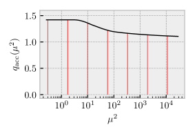
The input data is more ambiguous. It has to be a trade-off between precisely describing the variation and using as few data points as possible. Our input is a real vector of size $N_{\text{in}}$ obtained by sampling the acceptance function $q_{\text{acc}}^{k}(\mu^{2})$ defined in Eq. (5b) at a set of discrete points $\mu^{2}_{\ell}$, where $\ell=1,\ldots,N_{\text{in}}$. We use a logarithmic distribution of $\mu^{2}$ points for the sampling (i.e. with more points for lower scales), because the $\alpha_{\text{S}}$ ratios we will be using change more quickly for lower scales. Note that $q_{\text{acc}}^{k}$ also appears in the reweighting function for rejected events $q_{\text{rej}}^{k}$, cf. Eq. (5c), and therefore at least partly specifies how to vary rejected emissions.

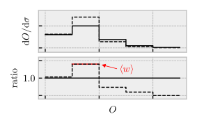
For illustration purposes, we show visualisations of these input/output choices in Fig. 1. The panel on the left shows the function $q_{\text{acc}}$, the red lines correspond to the values of $\mu^{2}$ at which we sample the function for the input vector. The shift in the observable in each bin is reported in the panel on the right, where the solid line shows the value of the observable for the nominal value of the parameters $\theta$, and the dotted line shows the shift that is observed for a variation of such parameters. The NN output needs to reproduce the shift in the ratio of the nominal value and the variation value.

(a) Neural net input data example

(b) Corresponding neural net output data

Figure 1: Visualisations of the neural network input/output data for a given observable bin (here the second bin in the histogram for an observable $O$, depicted in the right-hand panel). Given a number of values of $q_{\text{acc}}$ for a variation (left-hand panel) as input, the NN is trained such that it outputs the corresponding value $\langle w\rangle$ for the given bin.

3.3 Neural-network architecture and training

For our neural-network implementation and training we we use the PyTorch python library [54].

The input data is fed into a layer that consists of $N_{\text{in}}=60$ neurons that are linear modules, i.e. they compute their output using a linear function $y=mx+c$ from the input $x$, with the weight $m$ and the bias $c$ being trainable variables. As we have discussed in the previous section, the input $x$ is given by one of $N_{\text{in}}$ function values of the $q_{\text{acc}}^{k}$ function.

The input layer is fully connected to the next layer, which consists of 15 neurons that are rectifier linear units (ReLU). Given a value $x$ from the input layer, they pass on the value $y=\max(0,x)$ to the output layer. It is this hidden layer that introduces a non-linearity to the network, which is surely required for the problem at hand, given Eqs. (5).

The ReLU layer is then fully connected to the output layer which is just a single neuron. It is a linear module like the ones in the input layer. Its output $y$ gives the neural-network prediction for $\langle w_{k}\rangle_{b}$, i.e. $y=\langle w_{k}\rangle_{b}^{\text{NN}}$.

The training is done by minimizing the squared Euclidean distance between $\langle w_{k}\rangle_{b}^{\text{NN}}$ and the training data $\langle w_{k}\rangle_{b}$ for a range of different variations $k\in\mathcal{T}$, where $\mathcal{T}$ specifies the training data set. The loss function is defined as

$$\mathcal{L}=\sum_{k\in\mathcal{T}}\left[\langle w^{(k)}\rangle_{b}^{\text{NN}}-\langle w^{(k)}\rangle_{b}\right]^{2}\,.$$ (6)

The optimisation step is performed using the Adam algorithm [55] as implemented in PyTorch, with a learning rate of $10^{-4}$. The learning passes are performed until either a preset optimisation target (Euclidean distance $\leq 10^{-5}$) or a maximum number of passes ($10^{6}$) is reached. On a $2.8\text{\,}\mathrm{G}\mathrm{H}\mathrm{z}$ Core i7 processor this caps the CPU time for a training at approximately $30\text{\,}\mathrm{s}$, although depending on the training data and on the random initialization, it can also take only a few seconds. If necessary, the training time could be further reduced by using the GPU acceleration supported by PyTorch.

Every 5000 optimisation steps it is checked if the loss function has reduced by at least $0.1\text{\,}\mathrm{\char 37\relax}$. If this is not the case for five subsequent checks, the training is cancelled, assuming that a stable minimum has been found. If this minimum is however associated with a loss function value that is greater than $1\text{\,}\mathrm{\char 37\relax}$, the whole training pass is discarded and repeated with a newly randomised set of NN weights. Enforcing this threshold ensures that we do not accept trainings that have become stuck in a non-global minimum.

4 Validation

4.1 Validation procedure and training data

In this section we compare neural-network predictions $\langle w_{k}\rangle_{b}^{\text{NN}}$ with the true reweighting factor $\langle w_{k}\rangle_{b}$ for a range of different variations $k\in\mathcal{T}$ and observable bins $b$ (which are defined below). In doing that we will always exclude the data point that we want to predict from the trainings.

First, we generate $10^{6}$ parton-shower histories with the simplified model described in Sec. 3.1 and bin them one-by-one into a bin $b$ for each observable. For each observable bin $b$ and variation $k$, we calculate $\langle w_{k}\rangle_{b}$. These values will be the output data sample for the training/comparison of our neural networks.

As the input data sample, we calculate $N_{\text{in}}=60$ function values for $q_{\text{acc}}^{k}(\mu^{2})$ for each variation $k\in\mathcal{T}$, distributed logarithmically between the lowest scale $\min(\mu^{2})=t_{\text{IR}}/4$ reachable by the shower and $\mu_{t_{0}}+2\sigma_{t_{0}}$, i.e. including large $\mu^{2}$ values up two standard deviations $\sigma_{t_{0}}$ from the mean of the starting scale distribution $\mu_{t_{0}}$.

The general training procedure described in Sec. 3.3 is amended for the validation as follows. For predicting $\langle w_{k^{\prime}}\rangle_{b^{\prime}}$ for a given variation $k^{\prime}$ and histogram bin $b^{\prime}$, we use all the input and output data for $b^{\prime}$ and all $k\in\mathcal{T}$ except for $k=k^{\prime}$. Note that this means that we repeat the training for each $k\in\mathcal{T}$ (because we do not want to include the data for $k^{\prime}$ in the validation). In an application on the other hand, only one neural network for each observable bin $b$ would need to be trained to interpolate between the $k$.

Lastly, we repeat this $N_{\text{trainings}}=10$ times, each with randomly initialised neural net weights. Our neural net prediction for $(k^{\prime},b^{\prime})$ is then given by the mean of the outputs of these 10 neural nets given the values for $q_{\text{acc}}^{k^{\prime}}$ as input. As an uncertainty, we give the standard deviation for these 10 values.

Now let us define the training data set $\mathcal{T}$. The variations used in the training should be diverse enough to allow the neural net to predict other variations accurately. We include two classes of variations of $\alpha_{\text{S}}$:

$$\alpha_{\text{S}}(\mu^{2}) \rightarrow\alpha_{\text{S}}(s\,\mu^{2})\,,\qquad s =0.25\dots 4.00\,,$$ (7)

$$\alpha_{\text{S}}(\mu^{2}) \rightarrow\alpha_{\text{S}}(\mu^{2}\,|\,\alpha_{\text{S}}(m_{Z}^{2})=a)\,,\qquad a =0.108\dots 0.124\,,$$ (8)

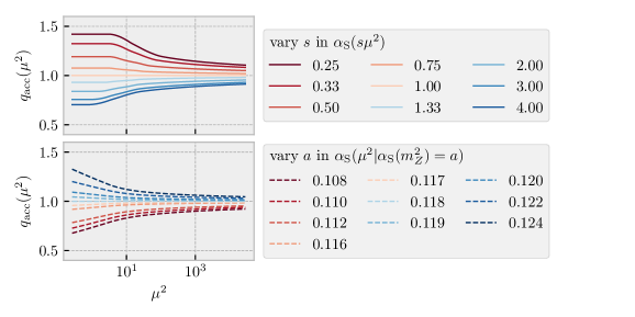
where $\alpha_{\text{S}}(\mu^{2}\,|\,\alpha_{\text{S}}(m_{Z}^{2})=a)$ is defined to be the strong coupling value at $\mu^{2}$ given that the value at the $Z$-boson mass, $\alpha_{\text{S}}(m_{Z}^{2})$, is set to $a$. For convenience we retrieve all $\alpha_{\text{S}}$ values we use from nnpdf 3.1 sets [1] interfaced using lhapdf [56]. This also dictates our choice of $a=\alpha_{\text{S}}(m_{Z})$ variations, since we use the values available in that nnpdf release. The individual values of $s$ and $a$ used in the validation and the corresponding $q_{\text{acc}}$ functions are shown in Fig. 2.

Figure 2: Display of the $\alpha_{\text{S}}$ variations used for validating the neural network approach. The upper row shows the scale variations, whereas the lower row shows variations of the input value $\alpha_{\text{S}}(m_{Z}^{2})$. The $q_{\text{acc}}$ function values as shown on the left are the input for the neural nets, as explained in Sec. 3.2.

4.2 Results

We discuss the results for the validation strategy laid down in this section so far for histogram bins of two observables: the scale $t^{\text{lead}}$ of the first emission in a parton-shower history, and the number of accepted emissions $N_{\text{em}}$ in a history. Note that these observables are not physical (as we use no jet algorithm), but merely serve here to test our approach.

Leading emission scale

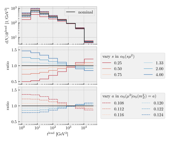
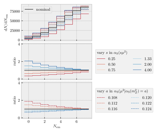
The first observable is the scale of the hardest emissions $t^{\text{lead}}$, binned into a histogram of 8 logarithmically distributed bins between 1 and $3\cdot 10^{4}$ GeV². The $t^{\text{lead}}$ distribution for the nominal $\alpha_{\text{S}}$ values and a subset of variations is shown in Fig. 3. The ratios between the NN result for the reweighting factor $\langle w_{k}\rangle_{b}^{\text{NN}}$ and the true value $\langle w_{k}\rangle_{b}$ are shown in Fig. 4, for all variations $k$ and observable bins $b$.

For the interpretation of this figure, note that we actually display ratios of ratios, i.e. the deviation between reweighting factors, that are itself just ratios of the nominal and the varied cross section. To calculate how far we are off relative to the absolute value of the cross section, one would need to multiply the true reweighting factor with the ratio in Fig. 4.

It is clear from the plots that the NN results are within $1\text{\,}\mathrm{\char 37\relax}$ of the true reweighting factor, and the uncertainty of the prediction is $\pm$3\text{\,}\mathrm{\char 37\relax}$$ or less. Exceptions only appear for the $s=0.25$ variation at small values of $t^{\text{lead}}$. Note that $s=0.25$ is an extremal variation, and hence in our validation procedure (where the to-be-predicted point is not included in the training data set) the NN needs to extrapolate when predicting this reweighting factor. The training data set should therefore go beyond the variations that are to be expected in an application, such that all NN predictions are guaranteed to be interpolations.

Figure 3: The effect of parton-shower $\alpha_{\text{S}}$ variations on the distribution of the leading emission scale $t^{\text{lead}}$. The lower two panels show the ratios broken down into scale variations and $\alpha_{\text{S}}(m_{Z}^{2})$ variations, respectively. Some intermediate variations that are used for the validation are left out here for clarity. The black line (“nominal”) gives the distribution for the nominal $\alpha_{\text{S}}$ choice, i.e. for $s=1$ and $a=0.118$.

Figure 4: Ratios between neural-net-predicted and true reweighting factors for each bin of the $t^{\text{lead}}$ histogram, see Fig. 3. Each row corresponds to one bin, with the smallest-$t^{\text{lead}}$ bin at the top. The two columns correspond to scale and $\alpha_{\text{S}}(m_{Z}^{2})$ variations.

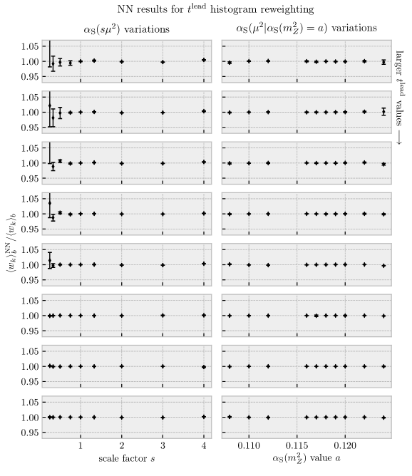
We have also tested how the uncertainties of the prediction behave when we initialise the NN weights with the same random numbers for each repetition of the training procedure. In that case, the spread becomes negligible compared to the results in Fig. 4. This means that the spread is not due to the numerical precision (floating point precision), but due to the random initialisation. Hence, in order to get even more precise predictions, the NN architecture and/or training procedure would have to be modified.

Number of emissions

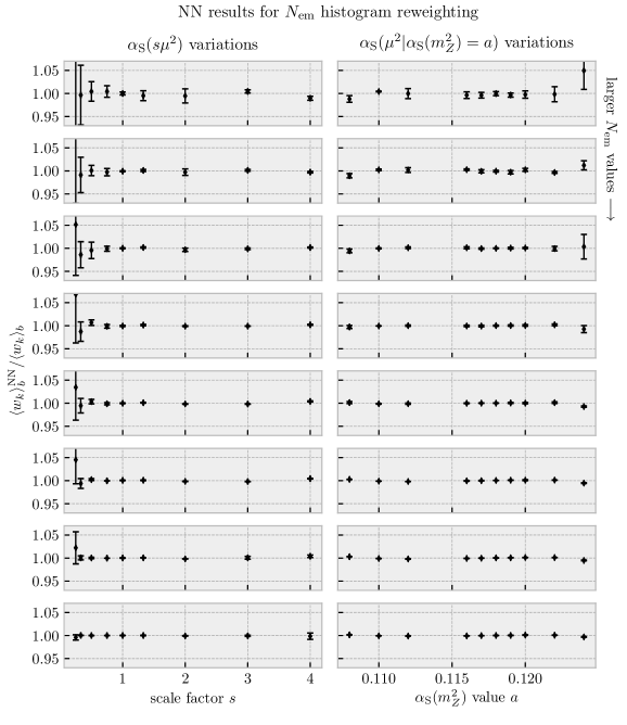
We also test our approach with the number of emissions, in 8 bins between 0 and 7 emissions. As for the $t^{\text{lead}}$, we show the $N_{\text{em}}$ histogram with all variations in Fig. 5, and the ratios for the reweighting factors given by the neural network and the training data in Fig. 6.

As for the $t^{\text{lead}}$ case we find that the neural network predictions are within $1\text{\,}\mathrm{\char 37\relax}$ of the true reweighting factor, with an uncertainty that only for some cases exceeds $3\text{\,}\mathrm{\char 37\relax}$. The exceptions occur in the region for variations that enhance emission probabilities (small $s$ and/or large $a$), in particular for bins with smaller $N_{\text{em}}$ values.

Figure 5: The effect of parton-shower $\alpha_{\text{S}}$ variations on the distribution of the number of emissions $N_{\text{em}}$. The lower two panels show the ratios broken down into scale variations and $\alpha_{\text{S}}(m_{Z}^{2})$ variations, respectively. See Fig. 3 for additional notes.

Figure 6: Ratios between neural-net-predicted and true reweighting factors for each bin of the $N_{\text{em}}$ histogram, see Fig. 5. Each row corresponds to one bin, with the smallest-$N_{\text{em}}$ bin at the top. The two columns correspond to scale and $\alpha_{\text{S}}(m_{Z}^{2})$ variations.

Further tests

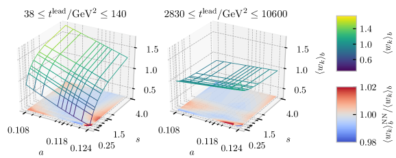
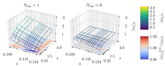
In Fig. 7(a) (7(b)) we present the absolute reweighting factors for a low- and a high-$t^{\text{lead}}$ ($N_{\text{em}}$) bin. Here we also include simultaneous variations (i.e. both $s\neq 1.0$ and $a\neq 0.118$), the training data set is defined by all pairs $(a,s)\in A\otimes S$ with the $\alpha_{\text{S}}(m_{Z}^{2})$ values $A=\{0.108,0.110,0.112,0.116,0.117,0.118,0.119,0.120,0.122,0.124\}$ and the scale factors $S=\{0.25,0.5,1.0,1.5,2.0,4.0\}$. The ratio of the NN result over the true reweighting factor is shown as a projection below the absolute reweighting factors. To calculate this, we use the same validation method as before, i.e. the predicted reweighting factor is left out in the training of the NN that is used for this point. We find that the deviations are within $2\text{\,}\mathrm{\char 37\relax}$ for simultaneous variations, except for the variation $a=0.124$, $s=0.25$, for which emission probabilities are maximally enhanced and $q_{\text{acc}}$ is most non-linear. This findings are also true for the bins that are not shown in the figure.

(a) leading emission scale $t^{\text{lead}}$

(b) number of emissions $N_{\text{em}}$

Figure 7: The reweighting factors for a low- and a high-$t^{\text{lead}}$ ($N_{\text{em}}$) bin are shown in the upper (lower) row. The projections on the $a$-$s$ plane show the ratio between neural-net-predicted and true reweighting factors, $\langle w_{k}\rangle_{b}^{\text{NN}}/\langle w_{k}\rangle_{b}$. The predicted factor was omitted in the training of the corresponding neural net. The clipped corners in the ratio projection for the $t^{\text{lead}}$ bins and the $N_{\text{em}}=1$ bin are due to the ratio being beyond the scale of $\pm$2\text{\,}\mathrm{\char 37\relax}$$ for $a=0.124$ and $s=0.25$.

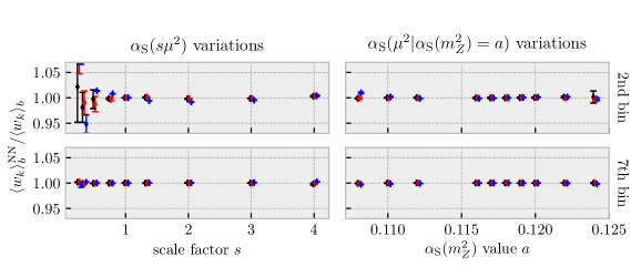
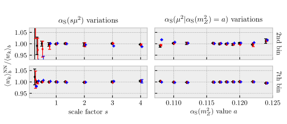
Finally, Fig. 8 shows the behaviour of the neural-network prediction when reducing the number of neurons. For this study, we return to our original training data set $\mathcal{T}$ that does not include simultaneous variations. We compare our previous choice of $N_{\text{in}}=60$ with using $N_{\text{in}}=40$ and $N_{\text{in}}=5$. The hidden layer always has $N_{\text{in}}/4$ neurons (which is rounded down to 1 for the $N_{\text{in}}=5$ case). Again, we only show two representative bins for both observables for the sake of brevity. Although $N_{\text{in}}=40$ only shows a minor degradation with respect to $N_{\text{in}}=60$ it features a substantially increased uncertainty for the low-$N_{\text{em}}$ bin and low values of the scale factor $s$. For $N_{\text{in}}=5$ we find significant deviations from unity, although even in this case only the low-$N_{\text{em}}$ bin features a deviation that is larger than $5\text{\,}\mathrm{\char 37\relax}$ (other than the extremal variations). These findings suggest that $N_{\text{in}}=60$ can probably be reduced while preserving enough precision and accuracy. However, we intend to use the validated architecture in an example more similar to potential applications in the following section. For that, we use a full parton-shower implementation, for which we foresee a stronger variation between the $q_{\text{acc}}(\mu^{2})$ values. Hence we keep $N_{\text{in}}=60$ as our baseline architecture.

(a) leading emission scale $t^{\text{lead}}$

(b) number of emissions $N_{\text{em}}$

Figure 8: Ratios between neural-net-predicted and true reweighting factors for a low- and a high-$t^{\text{lead}}$ ($N_{\text{em}}$) bin are shown in the upper (lower) two rows, using $N_{\text{in}}=60$ (black), 40 (red) and 5 (blue) input neurons. The hidden layer of ReLU is in each case set to have $N_{\text{in}}/4$ neurons (rounding down to the next integer).

5 A real-world example: varying Sherpa shower predictions for Thrust

We now study if the toy shower results from the previous sections can be transferred to a setup with a complete parton shower implementation and a real observable, namely the event shape observable Thrust for the process $e^{+}e^{-}\to\text{2 or more jets}$, simulated at a centre-of-mass energy of $91.2\text{\,}\mathrm{GeV}$.

We generate Monte-Carlo events for this process using the Sherpa event generator [10] and its Catani-Seymour Shower implementation (css) [57]. Non-perturbative effects (such as fragmentation and multiple interactions) and electroweak corrections are disabled. The $e^{+}e^{-}\to q\bar{q}$ matrix element is evaluated at leading-order in the couplings. The perturbative order of the running strong coupling is set to include up to two loops. The shower starting scale is set to the $Z$ mass, i.e. $\mu_{\text{Q}}=m_{Z}^{2}=($91.28\text{\,}\mathrm{GeV}$)^{2}$. The events are analysed using the Rivet analysis framework [58].

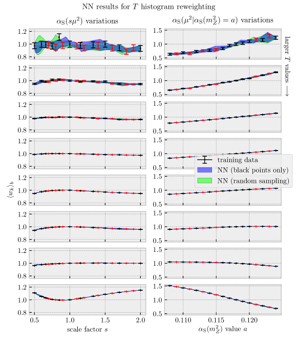
The set of variations used for the training is listed in Tab. 1. Instead of leaving out single training values as we did for the validation, we use the full training data set $\mathcal{T}$ and compare the predictions later with several variations that are not part of $\mathcal{T}$. The $N_{\text{in}}=60$ function values for $q_{\text{acc}}$ used as the input data are written out from within the css coupling implementation. The output data is given by generating the Thrust distribution for each variation and then calculating the ratio to the central value ($s=1.0$, $a=0.118$) for each bin. Some of the bins for lower Thrust values have a sizeable Monte-Carlo error. To take this into account, we train 20 neural network replicas per bin, and for each training we generate a new $\langle w_{k}\rangle_{b}$ replica over $k$. For each replica we vary the $\langle w_{k}\rangle_{b}$ values according to their central value and uncertainty, assuming a Gaussian distribution.

Table 1: List of variations used for training in the example application.

scale $s$	0.50	0.60	0.66	0.75	0.85
	1.15	1.33	1.50	1.70	2.00
$a=\alpha_{\text{S}}(m_{Z}^{2})$	0.108	0.110	0.112	0.114	0.116
	0.117	0.119	0.120	0.122	0.124

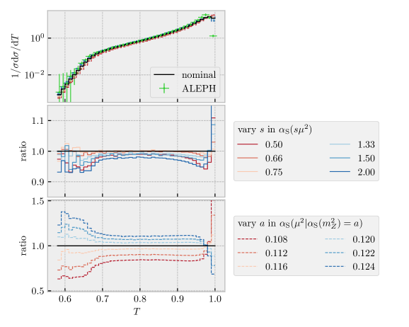
In Fig. 9, we show the LO+parton-shower prediction for Thrust and a selection of variations for both the scale factor $s$ and for $a=\alpha_{\text{S}}(m_{Z}^{2})$, and compare it with data by the aleph collaboration [59]. All reweighting factors for a representative selection of bins are shown in Fig. 10, along with the prediction for the entire variation ranges by the NN. This prediction reproduces the reweighting factors that were used to train the networks (black) and also the factors that are shown as control points (red). The uncertainties of the prediction follow the Monte-Carlo errors of the training reweighting factors. We also train a second set of NN, where we omit for each training pass a random selection of 7 variations in the training (but keeping the most extremal variations). The resulting band (green) also reproduces the data.

Note that each NN corresponds to one row in Fig. 10 (i.e. to one observable bin), and therefore predicts the different functional forms for both the $a$ and the $s$ variations. The facts that these functions are non-linear and that their forms depend on the variation type and observable bin suggest that an ordinary fit with a fixed parametrisation is not suitable for the task.

Figure 9: The effect of the sherpa Catani-Seymour shower variations on the distribution of the Thrust event shape observable. The nominal prediction ($a=0.118$, $s=1.0$) is shown in black, whereas the variations are colour-coded as listed in the legend on the right. The lower panels show the scale and $\alpha_{\text{S}}(m_{Z})$ variations, respectively. Some intermediate variations that are used in the NN training and comparison are left out to prevent that the plots become too busy. In the upper panel, we also show data points from the aleph collaboration [59].

Figure 10: A comparison between NN-predicted and true reweighting factors for a sample of bins of the Thrust $T$ histogram, see Fig. 9. Each row corresponds to one bin, with $T$ being in the intervals (0.58, 0.59), (0.63, 0.64), (0.88, 0.89), (0.96, 0.97), (0.97, 0.98), (0.98, 0.99), (0.99, 1.00) (from top to bottom). The data points correspond to the true reweighting factors and their Monte-Carlo errors. The black ones are used to train a first set of neural networks (blue band). A random sample omitting 7 points for each variation type is used to train a second set of neural networks (green band). The most extreme variations are always kept in the training set. The uncertainties corresponds to the Monte-Carlo error of the training data as described in the text.

6 Conclusions

Parton-shower calculations are currently not included in PDF fits, because of the CPU time needed to re-evaluate the parton shower event-by-event for new input parameters, and in particular as the PDFs are changing in the fitting process.

In this paper we suggested to use neural networks to encode the dependences of the cross section in a given observable bin on the parton-shower input parameters. We showed that the ansatz is working when applied to variations of the strong coupling (and its input scale) used in the shower splittings, both for a simplified shower model and for the full shower implementation in sherpa. The observables we tested are the leading emission scale, the number of emissions and the Thrust event shape.

This successful proof of principle makes us confident that it is worth exploring the method further, to study more observables and variation types but in particular to generalise it to take into account the PDF dependence of initial-state shower splittings. This will surely require a more advanced neural-net architecture or at least considerably more neurons and training data points, because the dependence of the splitting kernels on the PDFs is more complicated, and because varying PDF sets can not be done in just one dimension. It is nonetheless worthwhile trying to implement a fast reweighting procedure for these processes, in order to extend the range of data that can be used in PDF fits.

Acknowledgements. We thank Juan Rojo for interesting comments on the manuscript. EB & LDD are supported by an STFC Consolidated Grant, ST/P0000630/1. LDD is also supported by a Royal Society Wolfson Research Merit Award, WM140078.

References

- [1] NNPDF Collaboration, R. D. Ball et al., “Parton distributions from high-precision collider data,” Eur. Phys. J. C77 no. 10, (2017) 663, arXiv:1706.00428 [hep-ph].
- [2] S. Dulat, T.-J. Hou, J. Gao, M. Guzzi, J. Huston, P. Nadolsky, J. Pumplin, C. Schmidt, D. Stump, and C. P. Yuan, “New parton distribution functions from a global analysis of quantum chromodynamics,” Phys. Rev. D93 no. 3, (2016) 033006, arXiv:1506.07443 [hep-ph].
- [3] L. A. Harland-Lang, A. D. Martin, P. Motylinski, and R. S. Thorne, “Parton distributions in the LHC era: MMHT 2014 PDFs,” Eur. Phys. J. C75 no. 5, (2015) 204, arXiv:1412.3989 [hep-ph].
- [4] S. Alekhin, J. Blumlein, and S. Moch, “The ABM parton distributions tuned to LHC data,” Phys. Rev. D89 no. 5, (2014) 054028, arXiv:1310.3059 [hep-ph].
- [5] J. Gao, L. Harland-Lang, and J. Rojo, “The Structure of the Proton in the LHC Precision Era,” Phys. Rept. 742 (2018) 1–121, arXiv:1709.04922 [hep-ph].
- [6] NNPDF Collaboration, R. D. Ball et al., “Parton distributions for the LHC Run II,” JHEP 04 (2015) 040, arXiv:1410.8849 [hep-ph].
- [7] Z. Nagy, “Next-to-leading order calculation of three-jet observables in hadron-hadron collision,” Phys. Rev. D68 (2003) 094002, arXiv:hep-ph/0307268 [hep-ph].
- [8] J. Alwall, R. Frederix, S. Frixione, V. Hirschi, F. Maltoni, O. Mattelaer, H. S. Shao, T. Stelzer, P. Torrielli, and M. Zaro, “The automated computation of tree-level and next-to-leading order differential cross sections, and their matching to parton shower simulations,” JHEP 07 (2014) 079, arXiv:1405.0301 [hep-ph].
- [9] J. M. Campbell, R. K. Ellis, and W. T. Giele, “A Multi-Threaded Version of MCFM,” Eur. Phys. J. C75 no. 6, (2015) 246, arXiv:1503.06182 [physics.comp-ph].
- [10] T. Gleisberg, S. Höche, F. Krauss, M. Schönherr, S. Schumann, F. Siegert, and J. Winter, “Event generation with SHERPA 1.1,” JHEP 02 (2009) 007, arXiv:0811.4622 [hep-ph].
- [11] T. Carli, D. Clements, A. Cooper-Sarkar, C. Gwenlan, G. P. Salam, F. Siegert, P. Starovoitov, and M. Sutton, “A posteriori inclusion of parton density functions in NLO QCD final-state calculations at hadron colliders: The APPLGRID Project,” Eur. Phys. J. C66 (2010) 503–524, arXiv:0911.2985 [hep-ph].
- [12] T. Kluge, K. Rabbertz, and M. Wobisch, “FastNLO: Fast pQCD calculations for PDF fits,” in Deep inelastic scattering. Proceedings, 14th International Workshop, DIS 2006, Tsukuba, Japan, April 20-24, 2006, pp. 483–486. 2006. arXiv:hep-ph/0609285 [hep-ph]. http://lss.fnal.gov/cgi-bin/find_paper.pl?conf-06-352.
- [13] fastNLO Collaboration, D. Britzger, K. Rabbertz, F. Stober, and M. Wobisch, “New features in version 2 of the fastNLO project,” in Proceedings, 20th International Workshop on Deep-Inelastic Scattering and Related Subjects (DIS 2012): Bonn, Germany, March 26-30, 2012, pp. 217–221. 2012. arXiv:1208.3641 [hep-ph]. http://inspirehep.net/record/1128033/files/arXiv:1208.3641.pdf.
- [14] L. Del Debbio, N. P. Hartland, and S. Schumann, “MCgrid: projecting cross section calculations on grids,” Comput. Phys. Commun. 185 (2014) 2115–2126, arXiv:1312.4460 [hep-ph].
- [15] E. Bothmann, N. Hartland, and S. Schumann, “Introducing MCgrid 2.0: Projecting cross section calculations on grids,” Comput. Phys. Commun. 196 (2015) 617–618.
- [16] V. Bertone, R. Frederix, S. Frixione, J. Rojo, and M. Sutton, “aMCfast: automation of fast NLO computations for PDF fits,” JHEP 08 (2014) 166, arXiv:1406.7693 [hep-ph].
- [17] L. de Oliveira, M. Kagan, L. Mackey, B. Nachman, and A. Schwartzman, “Jet-images – deep learning edition,” JHEP 07 (2016) 069, arXiv:1511.05190 [hep-ph].
- [18] J. Lin, M. Freytsis, I. Moult, and B. Nachman, “Boosting with Machine Learning,” arXiv:1807.10768 [hep-ph].
- [19] S. Macaluso and D. Shih, “Pulling Out All the Tops with Computer Vision and Deep Learning,” arXiv:1803.00107 [hep-ph].
- [20] A. Butter, G. Kasieczka, T. Plehn, and M. Russell, “Deep-learned Top Tagging with a Lorentz Layer,” arXiv:1707.08966 [hep-ph].
- [21] H. Luo, M.-x. Luo, K. Wang, T. Xu, and G. Zhu, “Quark jet versus gluon jet: deep neural networks with high-level features,” arXiv:1712.03634 [hep-ph].
- [22] T. Cheng, “Recursive Neural Networks in Quark/Gluon Tagging,” Comput. Softw. Big Sci. 2 no. 1, (2018) 3, arXiv:1711.02633 [hep-ph].
- [23] G. Louppe, K. Cho, C. Becot, and K. Cranmer, “QCD-Aware Recursive Neural Networks for Jet Physics,” arXiv:1702.00748 [hep-ph].
- [24] P. T. Komiske, E. M. Metodiev, and M. D. Schwartz, “Deep learning in color: towards automated quark/gluon jet discrimination,” JHEP 01 (2017) 110, arXiv:1612.01551 [hep-ph].
- [25] C. Shimmin, P. Sadowski, P. Baldi, E. Weik, D. Whiteson, E. Goul, and A. Søgaard, “Decorrelated Jet Substructure Tagging using Adversarial Neural Networks,” Phys. Rev. D96 no. 7, (2017) 074034, arXiv:1703.03507 [hep-ex].
- [26] T. Q. Nguyen, D. Weitekamp, D. Anderson, R. Castello, O. Cerri, M. Pierini, M. Spiropulu, and J.-R. Vlimant, “Topology classification with deep learning to improve real-time event selection at the LHC,” arXiv:1807.00083 [hep-ex].
- [27] E. M. Metodiev, B. Nachman, and J. Thaler, “Classification without labels: Learning from mixed samples in high energy physics,” JHEP 10 (2017) 174, arXiv:1708.02949 [hep-ph].
- [28] M. Abdughani, J. Ren, L. Wu, and J. M. Yang, “Probing stop with graph neural network at the LHC,” arXiv:1807.09088 [hep-ph].
- [29] J. Bendavid, “Efficient Monte Carlo Integration Using Boosted Decision Trees and Generative Deep Neural Networks,” arXiv:1707.00028 [hep-ph].
- [30] P. T. Komiske, E. M. Metodiev, B. Nachman, and M. D. Schwartz, “Pileup Mitigation with Machine Learning (PUMML),” JHEP 12 (2017) 051, arXiv:1707.08600 [hep-ph].
- [31] M. Paganini, L. de Oliveira, and B. Nachman, “CaloGAN : Simulating 3D high energy particle showers in multilayer electromagnetic calorimeters with generative adversarial networks,” Phys. Rev. D97 no. 1, (2018) 014021, arXiv:1712.10321 [hep-ex].
- [32] J. Ren, L. Wu, J. M. Yang, and J. Zhao, “Machine Learning Scan and Application in SUSY,” arXiv:1708.06615 [hep-ph].
- [33] J. W. Monk, “Deep Learning as a Parton Shower,” arXiv:1807.03685 [hep-ph].
- [34] J. Barnard, E. N. Dawe, M. J. Dolan, and N. Rajcic, “Parton Shower Uncertainties in Jet Substructure Analyses with Deep Neural Networks,” Phys. Rev. D95 no. 1, (2017) 014018, arXiv:1609.00607 [hep-ph].
- [35] S. Carrazza, R. Frederix, K. Hamilton, and G. Zanderighi, “MINLO t-channel single-top plus jet,” JHEP 09 (2018) 108, arXiv:1805.09855 [hep-ph].
- [36] V. N. Gribov and L. N. Lipatov, “Deep inelastic e p scattering in perturbation theory,” Sov. J. Nucl. Phys. 15 (1972) 438–450. [Yad. Fiz.15,781(1972)].
- [37] G. Altarelli and G. Parisi, “Asymptotic Freedom in Parton Language,” Nucl. Phys. B126 (1977) 298–318.
- [38] Y. L. Dokshitzer, “Calculation of the Structure Functions for Deep Inelastic Scattering and e+ e- Annihilation by Perturbation Theory in Quantum Chromodynamics.,” Sov. Phys. JETP 46 (1977) 641–653. [Zh. Eksp. Teor. Fiz.73,1216(1977)].
- [39] V. V. Sudakov, “Vertex parts at very high-energies in quantum electrodynamics,” Sov. Phys. JETP 3 (1956) 65–71. [Zh. Eksp. Teor. Fiz.30,87(1956)].
- [40] S. Höche, F. Krauss, M. Schönherr, and F. Siegert, “A critical appraisal of NLO+PS matching methods,” JHEP 09 (2012) 049, arXiv:1111.1220 [hep-ph].
- [41] L. Lönnblad, “Fooling Around with the Sudakov Veto Algorithm,” Eur. Phys. J. C73 no. 3, (2013) 2350, arXiv:1211.7204 [hep-ph].
- [42] M. H. Seymour, “Matrix element corrections to parton shower algorithms,” Comput. Phys. Commun. 90 (1995) 95–101, arXiv:hep-ph/9410414 [hep-ph].
- [43] T. Sjöstrand, S. Mrenna, and P. Z. Skands, “PYTHIA 6.4 Physics and Manual,” JHEP 05 (2006) 026, arXiv:hep-ph/0603175 [hep-ph].
- [44] S. Plätzer and M. Sjodahl, “The Sudakov Veto Algorithm Reloaded,” Eur. Phys. J. Plus 127 (2012) 26, arXiv:1108.6180 [hep-ph].
- [45] S. Höche, S. Schumann, and F. Siegert, “Hard photon production and matrix-element parton-shower merging,” Phys. Rev. D81 (2010) 034026, arXiv:0912.3501 [hep-ph].
- [46] S. Mrenna and P. Skands, “Automated Parton-Shower Variations in Pythia 8,” Phys. Rev. D94 no. 7, (2016) 074005, arXiv:1605.08352 [hep-ph].
- [47] J. Bellm, S. Plätzer, P. Richardson, A. Siódmok, and S. Webster, “Reweighting Parton Showers,” Phys. Rev. D94 no. 3, (2016) 034028, arXiv:1605.08256 [hep-ph].
- [48] E. Bothmann, M. Schönherr, and S. Schumann, “Reweighting QCD matrix-element and parton-shower calculations,” Eur. Phys. J. C76 no. 11, (2016) 590, arXiv:1606.08753 [hep-ph].
- [49] R. Frederix, S. Frixione, V. Hirschi, F. Maltoni, R. Pittau, and P. Torrielli, “Four-lepton production at hadron colliders: aMC@NLO predictions with theoretical uncertainties,” JHEP 02 (2012) 099, arXiv:1110.4738 [hep-ph].
- [50] Z. Bern, L. J. Dixon, F. Febres Cordero, S. Höche, H. Ita, D. A. Kosower, and D. Maître, “Ntuples for NLO Events at Hadron Colliders,” Comput. Phys. Commun. 185 (2014) 1443–1460, arXiv:1310.7439 [hep-ph].
- [51] D. Maître, G. Heinrich, and M. Johnson, “N(N)LO event files: applications and prospects,” PoS LL2016 (2016) 016, arXiv:1607.06259 [hep-ph].
- [52] A. Buckley et al., “General-purpose event generators for LHC physics,” Phys. Rept. 504 (2011) 145–233, arXiv:1101.2599 [hep-ph].
- [53] S. Catani, B. R. Webber, and G. Marchesini, “QCD coherent branching and semiinclusive processes at large x,” Nucl. Phys. B349 (1991) 635–654.
- [54] A. Paszke, S. Gross, S. Chintala, G. Chanan, E. Yang, Z. DeVito, Z. Lin, A. Desmaison, L. Antiga, and A. Lerer, “Automatic differentiation in PyTorch,” in NIPS-W. 2017.
- [55] D. P. Kingma and J. Ba, “Adam: A method for stochastic optimization,” 1412.6980. https://arxiv.org/abs/1412.6980.
- [56] A. Buckley, J. Ferrando, S. Lloyd, K. Nordström, B. Page, M. Rüfenacht, M. Schönherr, and G. Watt, “LHAPDF6: parton density access in the LHC precision era,” Eur. Phys. J. C75 (2015) 132, arXiv:1412.7420 [hep-ph].
- [57] S. Schumann and F. Krauss, “A Parton shower algorithm based on Catani-Seymour dipole factorisation,” JHEP 03 (2008) 038, arXiv:0709.1027 [hep-ph].
- [58] A. Buckley, J. Butterworth, L. Lonnblad, D. Grellscheid, H. Hoeth, J. Monk, H. Schulz, and F. Siegert, “Rivet user manual,” Comput. Phys. Commun. 184 (2013) 2803–2819, arXiv:1003.0694 [hep-ph].
- [59] ALEPH Collaboration, A. Heister et al., “Studies of QCD at e+e- centre-of-mass energies between 91 and 209 GeV,” Eur. Phys. J. C35 (2004) 457–486.