Solution of the “sign problem” for the half filled Hubbard-Holstein model

Abstract

We show that, by an appropriate choice of auxiliary fields and exact integration of the phonon degrees of freedom, it is possible to define a ”sign-free” path integral for the so called Hubbard-Holstein model at half-filling. We use a statistical method, based on an accelerated and efficient Langevin dynamics, for evaluating all relevant correlation functions of the model. Preliminary calculations at $U/t=4$ and $U/t=1$, for $\omega_{0}/t=1$, indicate a quite extended region around $U\simeq{g^{2}\over\omega_{0}}$ without either antiferromagnetic or charge-density-wave orders, separating two quantum critical points at zero temperature. The elimination of the sign problem in a model without explicit particle-hole symmetry may open new perspectives for strongly correlated models, even away from the purely attractive or particle-hole symmetric cases.

Introduction: One of the most successful methods to obtain exact properties of strongly correlated models on a lattice is certainly the statistical (Monte Carlo) method based on the evaluation of a corresponding path integral defined in imaginary time. In particular most successful applications are based on auxiliary fields $\sigma_{l}^{j}$ introduced for each site $j$ of the model and imaginary time slice $l$ of the path integral by means of the so called “Hubbard-Stratonovich” transformation (HST) Blankenbecler et al. (1981); Hirsch (1983); Becca and Sorella (2017); Assaad (2005). Since the Hirsch seminal work in ’85 Hirsch (1985), several models have been studied, and their phase diagrams have been solved numerically for large enough number $N$ of sites, in very particular cases when the so called sign problem does not affect the simulation of the corresponding partition function $Z=\int\left[d\sigma_{l}^{j}\right]W(\left\{\sigma_{l}^{j}\right\})$, that is evaluated by standard statistical methods, as long as $W(\left\{\sigma_{l}^{j}\right\})\geq 0$. The first example was the Hubbard model in the square lattice, displaying a trivial phase diagram for the insulating antiferromagnetic phase, that turned out to be stable as soon as $U>0$. More recently the method was extended to the honeycomb lattice displaying a less trivial transition at a critical value $U_{c}$ between a semimetallic and an antiferromagnetic insulating or superconducting phase Sorella and Tosatti (1992); Sorella et al. (2012); Otsuka et al. (2016, 2018). Other models are worth to be mentioned such as, the negative-$U$ model Scalettar et al. (1989); Karakuzu et al. (2018), the spinless fermions with repulsive nearest-neighbors interaction at half filling Huffman and Chandrasekharan (2014); Li et al. (2015), the Anderson impurity model at half filling Hirsch and Fye (1986); Feldbacher et al. (2004), the Kondo-lattice model at half filling Assaad (1999); Capponi and Assaad (2001), the Holstein-model Hirsch and Fradkin (1983) and several others.

Most of the models so far solved without sign problem are characterized by i) an explicit spin-independent attractive interaction and/or ii) a particular particle-hole symmetry of the electronic degrees of freedom, implying that the corresponding weight $W(\{\sigma_{l}^{j}\})$ in the path-integral formulation can be written as the square of a quantity, and therefore positive. All these models have been recently classified in Ref. Wang et al. (2015); Li et al. (2016). For instance in the Hubbard model with $U>0$, the particle-hole transformation

$$c^{\dagger}_{i\downarrow}\to c_{i\downarrow}$$ (1)

( $c^{\dagger}_{i\downarrow}\to-c_{i\downarrow}$) for sites $i$ in the A (B) sublattice of a bipartite lattice, maps the positive-$U$ model to the negative-$U$ one with equal number of spin-up and spin-down electrons, where $c^{\dagger}_{j,\sigma}(c_{j,\sigma})$ creates (destroys) a fermion with spin $\sigma=\uparrow,\downarrow$ at a given site $j$. In such case the weight factorizes into two independent and identical contributions for different spins, thus $W(\{\sigma_{l}^{j}\})>0$.

The Hubbard-Holstein Hamiltonian is one of the simplest model describing the competition between an attractive interaction mediated by an optical phonon and the strong electron repulsion, defined by the Hubbard $U$, acting when two electrons of opposite spins occupy the same site. The Hubbard-Holstein model represents the key model to understand how the retarded interaction mediated by phonons can circumvent the strong electron-electron repulsion and give raise to superconductivity. It may be relevant not only to understand standard electron-phonon superconductivity, but also the high-temperature one, because the isotope effect has been clearly detected Hofer et al. (2000) in cuprates, and the so called kinks observed in photoemission experiments Lanzara et al. (2001) clearly indicate the role of phonons, even in these strongly correlated materials.

The phase diagram of the model has been studied using several techniques such as, Gutzwiller approximation Barone et al. (2008), variational Monte Carlo (VMC) Ohgoe and Imada (2017); Karakuzu et al. (2017), dynamical mean-field theory (DMFT) Werner and Millis (2007); Sangiovanni et al. (2006); Bauer and Hewson (2010), finite-temperature determinant quantum Monte Carlo (DQMC) Nowadnick et al. (2012); Johnston et al. (2013); Weber and Hohenadler (2018), also in 1D Hohenadler et al. (2012), but no unbiased zero temperature calculation is known in 2D.

In the present work we are able to establish ground-state benchmark results in the thermodynamic limit for this model, and some aspects of its zero-temperature phase diagram, by using a determinantal method, which, as we are going to show, is not vexed by the so called “sign problem”.

Model and Method: The Hubbard-Holstein model is defined by the following Hamiltonian:

$${\cal H} = {\cal H}_{\cal K}+{\cal H}_{\cal V},$$

$${\cal H}_{\cal K} = K+\frac{\omega_{0}}{2}\sum_{j}\hat{P}_{j}^{2},$$

$${\cal H}_{\cal V} = \frac{U}{2}\sum_{j}(n_{j}-1)^{2}+g\sum_{j}\hat{X}_{j}(n_{j}-1)+\frac{\omega_{0}}{2}\sum_{j}\hat{X}_{j}^{2}$$ (2)

$$= \frac{U}{2}\sum_{j}(n_{j}-1+{g\over U}\hat{X}_{j})^{2}+\frac{\omega_{0}-g^{2}/U}{2}\sum_{j}\hat{X}_{j}^{2},$$

where $K=-t\sum_{\langle i,j\rangle,\sigma}c^{\dagger}_{i,\sigma}c_{j,\sigma}+{\rm H.c.}$, $n_{j\sigma}=c^{\dagger}_{j,\sigma}c_{j,\sigma}$ indicates the electron number with spin $\sigma$ at the site $j$, and $n_{j}=\sum_{\sigma}n_{j\sigma}$. $t$ is the hopping integral, $U$ is the repulsive electron-electron interaction, whereas, $\omega_{0}$ is the phonon frequency, $g$ is the electron-phonon coupling term and, $\hat{X}_{j}$ and $\hat{P}_{j}$ are phonon position and momentum degrees of freedom, respectively.

At finite inverse temperature $\beta$ the partition function of an electronic system described by the Hamiltonian $\mathcal{H}$ is given by:

$$\mathcal{Z}={\rm Tr}[e^{-\beta\cal H}]={\rm Tr}[(e^{-\Delta\tau\cal H})^{T}],$$ (3)

where $\Delta\tau=\beta/T$ and the symbol ${\rm Tr}[O]$ associates a number to any operator $O$ and is defined by:

$${\rm Tr}[O]=\left\{\begin{array}[]{cc}{\rm Trace}[O]&{\rm for~{}the~{}standard~{}case}\\ \langle\Psi|O|\Psi\rangle&\text{ for ~{}the~{} projection~{}case}\end{array}\right.$$ (6)

where $\Psi$ is a chosen trial function, that may be conveniently introduced for evaluating the trace (up to an irrelevant constant) in the zero-temperature limit, as long as $\Psi$ has a non zero overlap with the ground state of ${\cal H}$. The latter case is known as zero-temperature projection, that is adopted in all the forthcoming calculations. However, for the sake of generality, we derive the method in the general case, as it is defined also within the more conventional finite-temperature scheme.

The imaginary-time propagator $e^{-\beta{\cal H}}$ can be written after Trotter decomposition as:

$$e^{-\Delta\tau\cal H}=e^{-\Delta\tau{\cal H}_{\cal V}}e^{-\Delta\tau{\cal H}_{\cal K}}+O(\Delta\tau^{2}),$$ (7)

In order to derive the path integral, the phonon degrees of freedom, introduced for each site $j$ and time slice $l$, are dealt as in a conventional Feynmann path integral where the phonon positions $X^{j}_{l}$ are changed at different time slices, just due to the phonon kinetic energy ${\omega_{0}\over 2}\sum\limits_{j}\hat{P}_{j}^{2}$, with associated matrix elements:

$$\langle X^{j}_{l+1}|\exp{\left(-{\Delta\tau\omega_{0}\over 2}\hat{P}_{j}^{2}\right)}|X^{j}_{l}\rangle\propto\exp{\left[-{1\over 2\omega_{0}\Delta\tau}(X^{j}_{l+1}-X^{j}_{l})^{2}\right]}$$ (8)

After that the operators $\hat{X}_{j}$ turn onto classical real variables $X_{j}^{l}$ to be integrated from $-\infty$ to $\infty$ in the corresponding path integral. For the remaining interaction term in ${\cal H}_{\cal V}$ we can use a properly chosen HST coupled to the operator $n_{j}-1+{g\over U}X_{l}^{j}$, namely:

$$e^{-\frac{U\Delta\tau}{2}(n_{j}-1+{g\over U}X_{l}^{j})^{2}}=\int_{-\infty}^{\infty}\frac{d\sigma_{l}^{j}}{\sqrt{2\pi}}e^{-\frac{1}{2}(\sigma_{l}^{j})^{2}+i\sqrt{U\Delta\tau}\sigma_{l}^{j}(n_{j}-1+{g\over U}X^{j}_{l})}$$ (9)

where $i$ is the imaginary constant, $\sigma_{j}^{l}$ are indicating the auxiliary fields in the $l^{\rm th}$ time slice. We thus get that the partition function can be expressed as a $2N\times T$ dimensional integral over the classical real variables $\sigma_{l}^{j}$ and $X_{l}^{j}$:

$$\mathcal{Z} = \bigintss\left[dX\right]\bigintss\left[d\sigma\right]\exp\left[-{1\over 2}\sum\limits_{l,m,j}\left(A_{l,m}X^{j}_{l}X^{j}_{m}+\delta_{l,m}(\sigma^{j}_{l})^{2}\right)\right]$$

$$\times {\rm Tr}\prod\limits_{l=1}^{T}\left\{\exp\left[\sum\limits_{j}\left(i\sqrt{U\Delta\tau}\sigma^{j}_{l}\right)(n_{j}-1+{g\over U}X^{j}_{l})\right]\exp(-\Delta\tau K)\right\}$$

where the product of non-commuting operators is meant from left to right with increasing $l$, $\left[dX\right]=\prod\limits_{j,l}dX_{l}^{j}$, $\left[d\sigma\right]=\prod\limits_{j,l}d\sigma_{l}^{j}$, and:

$$A_{l,m}={1\over\omega_{0}\Delta\tau}\left[2\delta_{l,m}-\delta_{l,m+1}-\delta_{m,l+1}\right]+\Delta\tau(\omega_{0}-g^{2}/U)\delta_{l,m}.$$ (11)

Here the boundary conditions for the phonon fields are $X^{j}_{l+T}=X^{j}_{l}$ for the standard finite temperature case (periodic in imaginary time) and $X^{j}_{0}=X^{j}_{T+1}=0$ for the projection case (open boundaries in imaginary time, within appropriate trial function $\Psi$ not (a)). In the path integral the dependence of the action on the fields $X_{l}^{j}$ is just quadratic and determined by the matrix $A$. After simple inspection, the eigenvalues of $A$ are given by

$$E_{n}={1\over\omega_{0}\Delta\tau}[2-2\cos(\omega_{n}\Delta\tau)]+\Delta\tau(\omega_{0}-g^{2}/U)$$ (12)

where $\omega_{n}\Delta\tau={2\pi n\over T}$ ($\omega_{n}\Delta\tau={n\pi\over T+1}$) for the finite temperature (projection) case and $n=1,\cdots T$. Therefore this matrix $A$ is positive definite ($E_{n}>0\forall n$) if $U>g^{2}/\omega_{0}$ and all the integrals in $\{X_{l}^{j}\}$ can be carried out before the $\{\sigma_{l}^{j}\}$ ones, as they are certainly converging:

$$\mathcal{Z} \propto \bigintss\left[d\sigma\right]\exp\left[-{1\over 2}\sum\limits_{l,m,j}\left(P_{l,m}\sigma^{j}_{l}\sigma^{j}_{m}\right)\right]$$

$$\times {\rm Tr}\prod\limits_{l}\left\{\exp\left[i\sqrt{U\Delta\tau}\sum\limits_{j}\sigma^{j}_{l}(n_{j}-1)\right]\exp(-\Delta\tau K)\right\}$$

where:

$$P_{l,m}=\delta_{l,m}+{\Delta\tau g^{2}\over U}\left[A^{-1}\right]_{l,m}.$$ (14)

is real and providing a positive weight in Eq. (LABEL:wght). On the other hand the remaining part contributing to the path integral weight $W(\{\sigma_{l}^{j}\})$, and resulting from the ${\rm Tr}$ operation is certainly positive, because the spin-up and spin-down contributions factorize and, after the particle-hole transformation in Eq. (1), turn out to be complex-conjugate factors [with appropriate $\Psi$ in the projection case]. Thus we have finally determined a path integral for the Hubbard-Holstein model with a positive real weight $W(\{\sigma_{l}^{j}\})>0$ for $U>g^{2}/\omega_{0}$.

A standard approach to evaluate correlation functions defined by the partition function $\mathcal{Z}$ is the Monte Carlo (MC) method. Unfortunately, the standard technique with local updates is very inefficient in this case, due to the difficulty to sample the stiff harmonic part. A better method was recently introduced Johnston et al. (2013), including global updates of the phonon fields. Global updates are numerically very demanding as they require the computation of several determinants from scratch. Here, in order to define an efficient sampling, we will use the first-order accelerated Langevin dynamics Parisi (1984), reviewed and generalized recently in Ref. Mazzola and Sorella (2017). The auxiliary fields at the $n^{\rm th}$ Markov chain iteration are updated via the discretized Langevin equation:

$$\vec{\sigma}_{n+1}=\vec{\sigma}_{n}+\Delta_{\rm MD}S^{-1}\vec{f}_{n}+\sqrt{2\Delta_{\rm MD}}S^{-1/2}\vec{z}_{n}$$ (15)

where $\vec{\sigma}=\{\bar{\sigma}_{j}^{l}\}$ are a shorthand notations for the fields represented as a $N\times T$ dimensional vector, $\Delta_{\rm MD}$ is the molecular-dynamics (MD) time step, $S_{l,m}^{i,j}$ is the acceleration matrix, that is chosen diagonal in the spatial indices $S_{l,m}^{i,j}=P_{l,m}\delta_{i,j}$ and corresponding to the harmonic classical part of the partition function, $\vec{z}_{n}$ are normally distributed random vectors, and $\vec{f}_{n}=\{f_{l}^{j}\}_{n}$ are generalized forces with components:

$$\{f_{l}^{j}\}_{n}=\partial_{\sigma_{l}^{j}}\ln(W(\{\sigma_{l}^{j}\}_{n})$$ (16)

It has been shown Beyl et al. (2018) that, within the complex auxiliary-field technique, the MD is free of ergodicity issues and we are able therefore to reproduce the results for the standard Hubbard model with $g=0$ (see Fig. 1), which represents the most difficult case in our approach as the acceleration matrix $S$ turns out to be the trivial identity matrix. Better choices should be possible but this study is beyond the main purpose of this work.

Results: In order to access the information about the order parameters we examine the charge and spin correlations of the model for different values of Hubbard interaction and electron-phonon coupling on $L\times L$ square lattices, at $\omega_{0}/t=1$.

We adopt the recently proposed dynamic scaling Weinberg and Sandvik (2017). We break the spin symmetry with the wavefunction $\Psi$, so that the antiferromagnetic order remains in the $z$ direction for the chosen projection times $\beta t=L$. The thermodynamic limit $\beta t=L=\infty$ remains unbiased, whereas the finite-size results do not recover the singlet finite-$L$ ground state, reachable only for much larger projection times. This technique, has the considerable advantage to allow very stable simulations without the so called “spikes” (samples of correlation functions much far from their average values) implying infinite variance problems Shi and Zhang (2016). Within this set up $m_{\rm AF}$ can be computed as:

$$m_{\rm AF}=\frac{1}{N}\sum_{i}{e^{i\textbf{Q}\cdot\textbf{r}_{i}}}\langle S_{i}\rangle$$ (17)

where $S_{i}=\frac{1}{2}(n_{i\uparrow}-n_{i\downarrow})$ is the value of the spin at site $i$ and the charge structure factor is given by:

$$S_{\rm CDW}(\textbf{Q})=\frac{1}{N}\sum_{i,j}{e^{i\textbf{Q}\cdot(\textbf{r}_{i}-\textbf{r}_{j})}}\langle n_{i}n_{j}\rangle$$ (18)

where $\langle\cdots\rangle={{\rm Tr}[\exp(-\beta H/2)\cdots\exp(-\beta H/2)]\over\mathcal{Z}}$, and the pitching vector ${\bf Q}=(\pi,\pi)$. We consider the evolution of these quantities as a function of the coupling $\lambda={g^{2}\over\omega_{0}}$. For $U\gg\lambda$ we have a Mott insulator with a finite antiferromagnetic (AF) order parameter $m_{\rm AF}>0$. As it is shown in Fig. 1(b) the dependence of this quantity on the MD time step $\Delta_{\rm MD}$ is rather smooth and can be safely extrapolated to the unbiased $\Delta_{\rm MD}\to 0$ limit. Similar behavior is obtained for all the other quantities considered in this work. The MD is particularly efficient just in the interesting region $\lambda\simeq U$ where phase transitions or at least competitions between antiferromagnetic, charge density wave or metallic and superconducting phases are expected Bauer and Hewson (2010). In this case, the chosen acceleration matrix is particularly efficient because it allows short correlation times $\simeq 1$ [see Fig.1(b) and inset] and very weak time step dependency, allowing large-scale simulations in this region.

As far as the systematic error implied by a finite Trotter time $\Delta\tau$, this becomes negligible provided measurements are evaluated at the middle of the kinetic-energy propagator $\exp(-\Delta\tau K)$ not (b), because in this way the error turns out quadratic in $\Delta\tau$. We have adopted $\Delta\tau t=0.1$ in all forthcoming calculations with an estimated error of less than $1\%$ in all quantities studied.

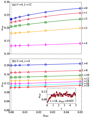
Figure 1: Antiferromagnetic order parameters $m_{\rm AF}$ at $U/t=4$ as a function of the MD time step $\Delta_{\rm MD}$ (a) on a 12 $\times$ 12 cluster at $\beta t=12$ and different values of the electron-phonon coupling strength $\lambda$. The $\lambda=\Delta_{\rm MD}=0$ result (filled circle) in (a) is obtained with the standard Monte Carlo algorithm for the Hubbard model, that is clearly consistent with the MD data, extrapolated to $\Delta_{\rm MD}\to 0$. (b) same as (a) for $\lambda=4$ with various system sizes $N=L\times L$, with $\beta t=L$. The inset shows the equilibration of $m_{\rm AF}$ to its average value (blue line) for the largest cluster as a function of the MD time $\tau$.

We have performed a finite-size scaling of $m_{\rm AF}$ and $S_{\rm CDW}({\bf Q})$ for $U/t=4$ and $U/t=1$ using clusters of size ranging from $6\times 6$ to $18\times 18$ for several couplings $\lambda\leq U$ and obtained the phase diagram reported in Fig. 2. As it is seen, the antiferromagnetic order drops continuously to much smaller values when we increase $\lambda$ and suggests a continuous transition to a non magnetic phase at $\lambda=\lambda_{c}^{\rm AF}\simeq U$. Within this assumption, and considering that the pure Holstein-model for $U=0$ (i.e. $\lambda\gg U$) displays charge-density-wave (CDW) order, $S_{\rm CDW}({\bf Q})$ should diverge for $\lambda\to\lambda_{c}^{\rm CDW}$ from below. Quite interestingly, the results reported in Fig. 2, suggest that $\lambda_{c}^{\rm CDW}$ is significantly larger than $\lambda_{c}^{\rm AF}$, because at small $U/t$ there is no evidence of the $S_{\rm CDW}({\bf Q})$ divergence, whereas for $U/t=4$, despite the fit of the data are consistent with a very small critical exponent $\theta$, $\lambda_{c}^{\rm CDW}$ is about 8% larger than $\lambda_{c}^{\rm AF}$. Indeed if we fix $\theta$ to a larger value in the fit, we obtain an even larger value of $\lambda_{c}^{\rm CDW}$.

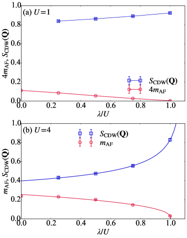
Figure 2: Ground state properties of the Hubbard-Holstein model obtained by extrapolating the antiferromagnetic order parameters to the thermodynamic limit for (a) $U$=1 and (b) $U$=4. The solid lines in (b) are the fit to $m_{\rm AF}$ and $S_{\rm CDW}(\bf{Q})$ of the form $\gamma\left(\frac{\lambda_{\rm c}-\lambda}{U}\right)^{\theta}$ with $\gamma$, $\theta$, and $\lambda_{\rm c}$ being the fitting parameters determined by the least-squares method. The parameters are found to be $\gamma=0.256(8)$, $\theta=0.39(5)$, and $\lambda_{\rm c}=\lambda_{\rm c}^{\rm AF}=4.02(2)$ for $m_{\rm AF}$ and $\gamma=0.407(2)$, $\theta=-0.286(12)$, and $\lambda_{\rm c}=\lambda_{\rm c}^{\rm CDW}=4.33(4)$ for $S_{\rm CDW}(\bf{Q})$.

Conclusions: In this work we have presented an original way to get rid of the sign problem in the Hubbard-Holstein model by using an appropriate auxiliary-field transformation combined with an exact integration of the phonon degrees of freedom. The Hubbard-Holstein model has been considered so far with algorithms affected by the sign problem, because, though at half filling, does not satisfy the particle-hole transformation in the electronic degrees of freedom:

$$c^{\dagger}_{j,\sigma}=(-1)^{j}c_{j,-\sigma}$$ (19)

where $(-1)^{j}=1$ ($-1$) if $j$ belongs to the A (B) sublattice. This transformation leaves unchanged the model without electron-phonon coupling but changes its sign when present. The key idea of this work is to employ an exact integration of the phonon degrees of freedom, that allow to recover this property and get rid of the sign problem, at least in a relevant parameter region $U>\lambda$. As we have shown the region $\lambda\simeq U$ is important because it is close to the phase transition of the model, and was previously inaccessible by numerical methods due to very severe sign problems Johnston et al. (2013). On the other hand in realistic materials the Coulomb energy is much larger than the electron-phonon coupling, as well as the phonon frequency $\omega_{0}$ and therefore the region $\lambda<U$, that can be studied with the present technique, is certainly the most important region for modelling realistic materials with the Hubbard-Holstein Hamiltonian.

Though the Hubbard-Holstein model is highly idealized, it is interesting to establish some benchmark results for the magnetic order parameter and the density structure factor (see Table 1). We see that our estimated $m_{\rm AF}$ compares well with the established benchmarks Qin et al. (2016) for $\lambda=0$, and remains approximately the same for $\lambda\ll U$, but with no evidence of CDW order, because $S_{\rm CDW}(\bf{Q})$ is clearly finite. Thus, as soon as $\lambda>0$, the electron-phonon coupling breaks the pseudo $SU(2)$ symmetry of the pure Hubbard model, and kills the CDW, leaving the AF order alone, in agreement with a rigorous theorem, recently proved Miyao . This feature reminds the phase diagram of the negative $U$ Hubbard model where the CDW order disappears immediately by a tiny amount of doping Scalettar et al. (1989).

Table 1: Values of $m_{\rm AF}$ and $S_{\rm CDW}(\textbf{Q})$ in the thermodynamic limits, for different values of $\lambda$, $U/t$ at $\omega_{0}=t$.

	$U/t=1$			$U/t=4$
$\lambda/U$	$m_{\rm AF}$	$S_{\rm CDW}(\bf{Q})$		$m_{\rm AF}$	$S_{\rm CDW}(\bf{Q})$
0	0.0280(2)	–		0.238(3)	–
0.25	0.0215(3)	0.838(4)		0.232(2)	0.433(7)
0.50	0.0138(3)	0.862(4)		0.202(4)	0.475(4)
0.75	0.0068(4)	0.890(5)		0.146(2)	0.557(9)
1	0.0009(1)	0.924(5)		0.031(2)	0.83(1)

Finally, since the transition to a non magnetic phase is very close to $\lambda\simeq U$, we have been able to determine some aspects of its phase diagram, namely that the transition is most likely continuous, at least up to $U/t=4$, as no evidence of a first order transition has been found for the $U$ values so far studied. Also, rather unexpectedly, an intermediate phase $\lambda_{c}^{\rm AF}\leq\lambda\leq\lambda_{c}^{\rm CDW}$ with no AF and CDW orders, appears rather robust and wide, in contrast with previous DMFT and VMC results.

This technique can be possibly extended to many other models, so far affected by the sign problem, and may open the way to tackle other important models where the particle-hole symmetry is not satisfied, first among all the Hubbard model at finite doping. Though we do not expect that the sign problem in this model can be definitively removed, this work certainly suggests that the sign of the weight $W(\{\sigma_{l}^{j}\})$ can be very likely improved, being a property of the appropriate auxiliary field chosen, and the degrees of freedom selected in the path integral, where enormous freedom has not been so far explored.