Straightforward integration for free surface Green function and body wave motions

Abstract

An alternative manner is provided for solving the classical linearised problem of the radiation and diffraction of regular water waves caused by oscillation of a floating body in deep water. It is shown that the singular wave integrals of the three-dimensional free surface Green function $G$ and its gradient $\nabla G$ can be regarded as regular wave integrals and are integrated directly. The method is validated by comparing with benchmark data for a floating or submerged body undergoing oscillatory wave motions. The comparison shows that the evaluation is sufficiently accurate for practical purposes. As the significance of the method, the numerical approximation stability for the gradient $\nabla G$ is shown to be the same with that for $G$.

1 Introduction

The determination of wave induced forces resulting from body wave motion is a fundamental problem in hydrodynamics. For the linear situation, the velocity potential of the fluid motion problem is a harmonic function and can be represented as a solution of body boundary integral equation involving the pulsating free surface Green function. The equation can be solved numerically by combining panel method and suitable approximation of the pulsating free surface Green function or free surface sources distributed on the body surface [1, 2, 3, 4, 5]. Varieties of Rankine simple source methods are also available to solve the body wave motion problems [6, 7, 8, 9, 10, 11] by using the dynamic and kinematic free surface boundary conditions rather than employing free surface Green functions. For a radial symmetric body undergoing oscillatory wave motion, its linear analytic solution can be approximated by a single free surface source rather than the boundary integral of free surface sources continuously distributed on the body surface. For a heaving or surging hemisphere, the velocity potential solution is decomposed into a free surface source located at the centre of the sphere and a wave-free potential, which is expanded in a series of Legendre polynomials and sinusoidal functions [12, 13, 14]. The unknown source strength and expansion coefficients are determined by the boundary condition of the velocity potential on the hemisphere. This method also applies to the wave resistance problem [15] of a travelling spheroid in waves and is available to the understanding of a submerged sphere in waves [16, 17, 18].

In the present study, we are interested in the approach of free surface Green function, which is evaluated in a straightforward manner. Consider a fluid of infinite water depth upper bounded by the average free water surface $z=0$ and consider a pulsating source $\bm{p}=(\xi,\eta,\zeta)$ with the unit strength undergoing periodic oscillatory motion with a constant frequency $\omega$ in the fluid. The velocity potential of the source measured at a field point $\bm{q}=(x,y,z)$ is expressed as

$$\Phi(\bm{q})=\frac{1}{4\pi}\mathrm{Re}(G(\bm{q},\bm{p})\mathrm{e}^{-\mathrm{i}\omega t}).$$

Here $G$ is known as the fundamental solution of the Laplace equation under a free surface boundary condition and a radiation condition or the pulsating free surface Green function [19, pages 476-477]

$$G\!\!\! =\!\!\! -\frac{1}{|\bm{q}-\bm{p}|}-\frac{1}{|\bm{q}-\bar{\bm{p}}|}-K(\bm{q},\bm{p})$$ (1)

for the singular wave integral

$$K=\frac{\nu}{\pi}\int^{\pi}_{-\pi}\int_{L}\frac{\mathrm{e}^{k(z+\zeta)+\mathrm{i}k(x-\xi)\cos\theta+\mathrm{i}k(y-\eta)\sin\theta}}{k-\nu}\mathrm{d}\theta\mathrm{d}k.$$ (2)

Here $\nu=\frac{\omega^{2}}{g}$ with $g$ the gravitational acceleration and $L$ illustrated by Figure 1 is an integration path passing beneath the singular wave number $k=\nu$.

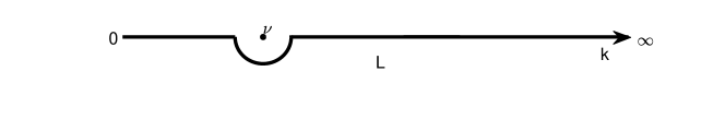
Figure 1: Profile of the integration path $L$ in (2) passing beneath the singular wave number $k=\nu$ in the complex plane.

On the other hand, if we consider a three-dimensional body undergoing periodic oscillatory motion with a constant frequency $\omega$ in the fluid, the velocity potential of the linearised oscillatory fluid motion problem can be represented as

$$\Phi=\mathrm{Re}(\phi\mathrm{e}^{-\mathrm{i}\omega t}),$$ (3)

where $\phi$ is a stationary complex potential satisfying the boundary integral equation

$$\phi(\bm{q})+\frac{1}{4\pi}\int_{S}\phi(\bm{p})\bm{n}\cdot\nabla G(\bm{q},\bm{p})\mathrm{d}S_{\bm{p}} = \frac{1}{4\pi}\int_{S}G(\bm{q},\bm{p})\bm{n}\cdot\nabla\phi(\bm{p})\mathrm{d}S_{\bm{p}}$$

$$= \frac{1}{4\pi}\int_{S}G(\bm{q},\bm{p})(-\mathrm{i}\omega n_{\alpha})\mathrm{d}S_{\bm{p}},$$

after the use of the impermeable body boundary condition

$$\bm{n}\cdot\nabla\phi=-\mathrm{i}\omega n_{\alpha}\,\,\mbox{ on }S.$$ (5)

Here $\nabla=(\partial_{\xi},\partial_{\eta},\partial_{\zeta})$ is derivative operator with respect to $\bm{p}$, $S$ is the average wetted surface of the body and $\bm{n}=\bm{n}(\bm{p})=(n_{1},n_{2},n_{3})$ represents the normal vector field of $S$ pointing into the fluid. The body undergoes heave motion for $\alpha=3$, sway motion for $\alpha=2$ and surge motion for $\alpha=1$.

Equations (1) and (5) show that the wave-body motion problem lies on the evaluation of the Green function $G$ and its gradient $\nabla G$ or the wave integral $K$ and its gradient $\nabla K$.

The present study is a continuation of the author’s previous examination on the pulsating free surface Green function [20] by integrating directly a regular wave integral. The method [20] is based on the approximation

$$K=\lim_{\mu\to 0+}K^{\mu}$$ (6)

with respect to the regular wave integral

$$K^{\mu}=\frac{\nu+\mathrm{i}\mu}{\pi}\int^{\infty}_{0}\int^{\pi}_{-\pi}\frac{\mathrm{e}^{k(z+\zeta)+\mathrm{i}k(x-\xi)\cos\theta+\mathrm{i}k(y-\eta)\sin\theta}}{k-\nu-\mathrm{i}\mu}\mathrm{d}\theta\mathrm{d}k.$$ (7)

As the normal derivative rather than the gradient is used in the boundary integral (1), we evaluate the normal derivative $\bm{n}\cdot\nabla G$ or $\bm{n}\cdot\nabla K$ instead of the gradient $\nabla G$ or $\nabla K$. By the mathematical definition of the Riemann integrals (7) and $\bm{n}\cdot\nabla K^{\mu}$, they can be approximated respectively as integrals of piecewise constant functions within flat panels. However, one may consider higher order approximations to the integrals. Integrating the regular wave integral (7) and the corresponding integral for $\bm{n}\cdot\nabla K^{\mu}$ straightforwardly, the evaluation is obtained as follows [20]

$$K = \sum_{i=1}^{\infty}\sum_{j=1}^{\infty}c_{i,j}\mathrm{e}^{k_{i}(z+\zeta)+\mathrm{i}k_{i}(x-\xi)\cos\theta_{j}+\mathrm{i}k_{i}(y-\eta)\sin\theta_{j}},$$ (8)

$$\bm{n}\cdot\nabla K = \sum_{i=1}^{\infty}\sum_{j=1}^{\infty}c_{i,j}^{\prime}k_{i}\mathrm{e}^{k_{i}(z+\zeta)+\mathrm{i}k_{i}(x-\xi)\cos\theta_{j}+\mathrm{i}k_{i}(y-\eta)\sin\theta_{j}}.$$ (9)

with respect to a small $\mu>0$, a set of mesh grid points $\{(k_{i},\theta_{j})|\,\,i=1,2,...,\infty;j=1,2,...,\infty\}$ of $[0,\infty)\times[-\pi,\,\pi]$ and the expansion coefficients

$$c_{i,j} = \frac{\nu+\mathrm{i}\mu}{\pi}(\theta_{j+1}-\theta_{j})\ln\frac{k_{i+1}-\nu-\mathrm{i}\mu}{k_{i}-\nu-\mathrm{i}\mu},$$ (10)

$$c_{i,j}^{\prime} = c_{i,j}[n_{3}-\mathrm{i}n_{1}\cos\theta_{j}-\mathrm{i}n_{2}\sin\theta_{j}].$$ (11)

This expansion gives rise to a simple evaluation of the Green function and, what is more, shows the structure of a free surface wave (see the free surface wave elevation produced by the source in [20, page 174]. That is, the singular wave integral is the superposition of all incident wave potentials

$$\mathrm{e}^{k_{i}(z+\zeta)+\mathrm{i}k_{i}(x-\xi)\cos\theta_{j}+\mathrm{i}k_{i}(y-\eta)\sin\theta_{j}}$$ (12)

in all incident angles $-\pi\leq\theta_{j}<\pi$ and wave numbers $0<k_{i}<\infty$.

However, it should be noted that the expansion (9) for the normal derivative of $\bm{n}\cdot\nabla K$ increases with the factor $k_{i}$. Thus the convergence stability of the $\bm{n}\cdot\nabla K$ expansion is very different to that of the $K$ expansion with respect to the free water surface $z+\zeta=0$.

It is the purpose of the present paper to introduce new expansion approximations of $K$ and $\bm{n}\cdot\nabla K$ so that the factor $k_{i}$ is removed and thus $\bm{n}\cdot\nabla K$ and $K$ have the same convergent property.

The singular wave integral (6) has been approximated by a variety of elementary function expansions (see, for example, [21, 22, 23, 24, 25]).

The use of the regular wave integral (7) dates back to the work of Havelock [26, 27] in 1920s on the regular wave integral

$$\frac{\nu}{\pi}\mathrm{Re}\int^{\pi}_{-\pi}\int^{\infty}_{0}\frac{\mathrm{e}^{k[z+\zeta+\mathrm{i}\cos(x-\xi)\cos\theta+\mathrm{i}(y-\eta)\sin\theta]}}{k\cos^{2}\theta-\nu-\mathrm{i}\mu\cos\theta}dkd\theta$$ (13)

for the translating free surface Green function with respect to an artificial viscosity number $\mu$. The regular wave integral

$$\frac{2\nu(1+\mathrm{i}\mu)^{2}}{\pi}\int^{\pi}_{0}\int^{\infty}_{0}\frac{\mathrm{e}^{k(z+\zeta)-\mathrm{i}k\sqrt{(x-\xi)^{2}+(y-\eta)^{2}}\cos\theta}}{k-\nu(1+\mathrm{i}\mu)^{2}}\mathrm{d}k\mathrm{d}\theta.$$ (14)

was also introduced in [22] to aid the evaluation of the pulsating free surface Green function in terms of exponential integrals via the decomposition of the singular wave integral into a near field flow component defined by the singular wave number $k=\nu$ or the dispersion relation $k-\nu=0$ and a far field flow component defined by the integral away from $k=\nu$. Further developments of this technique were obtained in [28, 29, 30] for analytic derivations of a non-oscillatory near field flow component $G^{N}$ (or $\phi^{N}$) and a far field wave component $G^{W}$ (or $\phi^{N}$) for the wave integral $G^{F}$ of a translating and pulsating free surface Green function (or a free surface effect component $\phi^{F}$ of a potential flow for a ship advancing in waves). The far field wave components are single integrals resulted from the integral along the domain defined by the poles of singular integral integrands. One may also refer to [31] on the translating Green function for the use of (13) for determining the uniqueness of the corresponding singular integral. Recent development of [22] for polynomial function approximation to the two flow components of the singular wave integral (6) was given in [25] and applied to a body wave motion problem [5].

The straightforward integration technique is initiated from [32], on the integration of the regular wave integral of the two-dimensional vortex free surface Green function, which is developed from the understanding of the instability of viscous flow in magnetohydrodynamics [33, 34] dominated by the Harmann layer friction controlled by the Hartmann number $\mu$. The limit (6) is used to assume $K=K^{\mu}$ for $0<\mu\ll 1$ throughout our examination. With the presence of the parameter $\mu>0$, the real part of the integrand of (7) is smooth and symmetric around the wave number $k=\nu$ and the corresponding imaginary part is smooth but close to a dirac delta function. Thus $K$ is integrable directly. In contrast to traditional evaluation schemes in earlier examinations, wave integral singularities are always a barrier in Green function evaluations as singular wave integrals are supposed to be not integrable directly.

The pulsating free surface Green function applies to radiation and diffraction wave problem defined by the boundary integral equation (1) without involving integration over the water line, the intersection contour of linear wetted body surface with average free water surface. However, if the body advancing at a uniform speed, the water line integral $\int_{\Gamma}(G\partial_{x}\phi-\phi\partial_{x}G)dl$ arises due to the integration by parts over free surface [35, 36]. Recently, a consistent boundary integrating formulation for ship advancing in calm water was given in [37, 38] showing that the troublesome water line integral of the function $G\partial_{x}\phi$ can be cancelled with the boundary integration over the defference between the linearised wetted body surface and the averaging wetted body surface.

2 Evaluation of the Green function

With the use of the Bessel function [39] of the first kind

$$J_{0}(kR) = \frac{1}{2\pi}\int^{\pi}_{-\pi}e^{\mathrm{i}k(x-\xi)\cos\theta+\mathrm{i}k(y-\eta)\sin\theta}d\theta=\frac{1}{2\pi}\int^{\pi}_{-\pi}e^{\mathrm{i}kR\sin\theta}d\theta$$

for $R=\sqrt{(x-\xi)^{2}+(y-\eta)^{2}}$, the singular wave integral $K$ of the Green function can be rewritten as [19, pages 476-477]

$$K = 2\nu\int_{L}\frac{\mathrm{e}^{k(z+\zeta)}}{k-\nu}J_{0}(kR)\mathrm{d}k.$$ (15)

Accordingly, the regular wave integral can be rewritten as

$$K^{\mu} = 2(\nu+\mathrm{i}\mu)\int^{\infty}_{0}\frac{\mathrm{e}^{k(z+\zeta)}}{k-\nu-\mathrm{i}\mu}J_{0}(kR)\mathrm{d}k.$$ (16)

In order to provide a convergent evaluation of the gradient $\nabla K$ on the free surface $z+\zeta=0$, we use the derivative of the Bessel function of the first kind [39]

$$J_{1}(x)=-\frac{dJ_{0}(x)}{dx}$$ (17)

and the elementary identity

$$\frac{k}{k-\nu-\mathrm{i}\mu}=\frac{\nu+\mathrm{i}\mu}{k-\nu-\mathrm{i}\mu}+1$$ (18)

to obtain

$$\frac{\partial K^{\mu}}{\partial R} =-2(\nu+\mathrm{i}\mu)\int^{\infty}_{0}\frac{e^{k(z+\zeta)}k}{k-\nu-\mathrm{i}\mu}J_{1}(kR)dk$$

$$=-2(\nu+\mathrm{i}\mu)^{2}\!\!\!\int^{\infty}_{0}\!\!\!\frac{e^{k(z\!+\!\zeta)}}{k\!-\!\nu\!-\!\mathrm{i}\mu}J_{1}(kR)dk\!-\!2(\nu\!+\!\mathrm{i}\mu)\int^{\infty}_{0}\!\!\!e^{k(z\!+\!\zeta)}J_{1}(kR)dk.$$ (19)

With the use of the derivative (17) and integration by parts, the second integral on the right-hand side of the previous equation can be modified as, for $z+\zeta<0$,

$$\int^{\infty}_{0}e^{k(z+\zeta)}J_{1}(kR)dk =-\frac{1}{R}\int^{\infty}_{0}e^{k(z+\zeta)}dJ_{0}(kR)$$

$$=-\frac{1}{R}\left[e^{k(z+\zeta)}J_{0}(kR)\right]^{kR=\infty}_{kR=0}+\frac{1}{R}\int^{\infty}_{0}\!\!\!J_{0}(kR)\frac{\partial\mathrm{e}^{k(z+\zeta)}}{\partial k}dk$$

$$=\frac{1}{R}+\frac{z+\zeta}{R}\int^{\infty}_{0}e^{k(z+\zeta)}J_{0}(kR)dk$$

$$=\frac{1}{R}+\frac{1}{R}\frac{z+\zeta}{\sqrt{R^{2}+(z+\zeta)^{2}}},\,\,\mbox{ since }z+\zeta<0,$$

$$=\frac{R}{\sqrt{R^{2}+(z+\zeta)^{2}}(\sqrt{R^{2}+(z+\zeta)^{2}}+|z+\zeta|)},$$ (20)

where we have used the identity

$$\frac{1}{\sqrt{R^{2}+(z+\zeta)^{2}}}=\int^{\infty}_{0}e^{k(z+\zeta)}J_{0}(kR)dk$$ (21)

due to two-dimensional Fourier transform on the $Oxy$ plane. Therefore, the combination of (19) and (20) gives

$$\frac{\partial K^{\mu}}{\partial R} = -2(\nu+\mathrm{i}\mu)^{2}\int^{\infty}_{0}\frac{e^{k(z+\zeta)}}{k-\nu-\mathrm{i}\mu}J_{1}(kR)dk$$ (22)

$$-\frac{2(\nu+\mathrm{i}\mu)R}{\sqrt{R^{2}+(z+\zeta)^{2}}(\sqrt{R^{2}+(z+\zeta)^{2}}+|z+\zeta|)}.$$

By (16) and (18), we have

$$\frac{\partial K^{\mu}}{\partial z} = 2(\nu+\mathrm{i}\mu)\int^{\infty}_{0}\frac{e^{k(z+\zeta)}k}{k-\nu-\mathrm{i}\mu}J_{0}(kR)dk$$ (23)

$$= 2(\nu+\mathrm{i}\mu)^{2}\int^{\infty}_{0}\frac{e^{k(z+\zeta)}}{k-\nu-\mathrm{i}\mu}J_{0}(kR)dk+2(\nu+\mathrm{i}\mu)\int^{\infty}_{0}e^{k(z+\zeta)}J_{0}(kR)dk$$

$$= (\nu+\mathrm{i}\mu)K^{\mu}+\frac{2(\nu+\mathrm{i}\mu)}{\sqrt{R^{2}+(z+\zeta)^{2}}}.$$

Let us note that the identity $\partial K/\partial z=\nu K+2\nu/\sqrt{R^{2}+(z+\xi)^{2}}$ is implied from [22, Eq. (9.3)].

On the other hand, for the regular wave integral $K^{\mu}$ , we use the Bessel function asymptotic behaviors

$$J_{0}(s)=O(\frac{1}{\sqrt{s}})\,\,\mbox{ and }\,\,J_{1}(s)=O(\frac{1}{\sqrt{s}})$$ (24)

with respect to large $s>0$ to obtain the convergence of the infinite domain integral

$$\int^{\infty}_{0}\frac{\mathrm{e}^{k(z+\zeta)}J_{n}(kR)}{k-\nu-\mathrm{i}\mu}\mathrm{d}k=\lim_{N\to\infty}\int^{N}_{0}\frac{\mathrm{e}^{k(z+\zeta)}J_{n}(kR)}{k-\nu-\mathrm{i}\mu}\mathrm{d}k,\,\,\,n=0,1.$$ (25)

Therefore, we may define $k_{\mathrm{max}}$ as a large number $N$. For a dense coordinate grid $\{k_{j}\}_{j=1}^{N_{k}}$ of the interval $[0,\,k_{\mathrm{max}}]$, we have

$$K^{\mu} = 2(\nu+\mathrm{i}\mu)\int^{k_{\mathrm{max}}}_{0}\frac{\mathrm{e}^{k(z+\zeta)}J_{0}(kR)}{k-\nu-\mathrm{i}\mu}\mathrm{d}k$$

$$= 2(\nu+\mathrm{i}\mu)\sum_{j=1}^{N_{k}}\int^{k_{j+1}}_{k_{j}}\frac{\mathrm{e}^{k(z+\zeta)}J_{0}(kR)}{k-\nu-\mathrm{i}\mu}\mathrm{d}k.$$

This yields, by the continuous function property of the integrand numerator,

$$K^{\mu} = 2(\nu+\mathrm{i}\mu)\sum_{j=1}^{N_{k}}\mathrm{e}^{k_{j}(z+\zeta)}J_{0}(k_{j}R)\int^{k_{j+1}}_{k_{j}}\frac{\mathrm{d}k}{k-\nu-\mathrm{i}\mu}$$ (26)

$$= 2(\nu+\mathrm{i}\mu)\sum_{j=1}^{N_{k}}\mathrm{e}^{k_{j}(z+\zeta)}J_{0}(k_{j}R)\ln\frac{k_{j+1}-\nu-\mathrm{i}\mu}{k_{j}-\nu-\mathrm{i}\mu}.$$

This also evaluates $\frac{\partial K^{\mu}}{\partial z}$ due to (23).

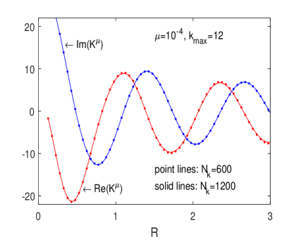
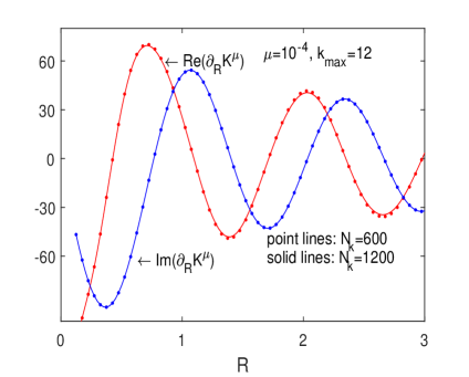
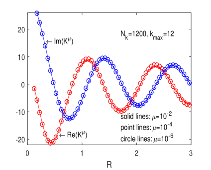
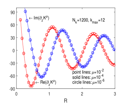
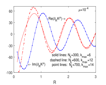
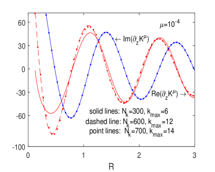
Figure 2: Convergence of the regular wave integral $K^{\mu}$ in (8) and its derivatives in (27) and (23) with respect to different parameters at $z=0$ and $\nu=5$.

Similarly, we have the partial derivative

$$\frac{\partial K^{\mu}}{\partial R} = -2(\nu+\mathrm{i}\mu)^{2}\sum_{j=1}^{N_{k}}\mathrm{e}^{k_{j}(z+\zeta)}J_{1}(k_{j}R)\ln\frac{k_{j+1}-\nu-\mathrm{i}\mu}{k_{j}-\nu-\mathrm{i}\mu}$$ (27)

$$-\frac{2R(\nu+\mathrm{i}\mu)}{\sqrt{R^{2}+(z+\zeta)^{2}}(\sqrt{R^{2}+(z+\zeta)^{2}}+|z+\zeta|)}.$$

Upon the observation

$$\lim_{\mu\to 0+}K^{\mu}=K,$$

we may assume $K=K^{\mu}$ for small $\mu>0$ and thus have the following approximations

$$K = \sum_{j=1}^{N_{k}}c_{j}\mathrm{e}^{k_{j}(z+\zeta)}J_{0}(k_{j}R),$$ (28)

$$\frac{\partial K}{\partial R} = -(\nu\!+\!\mathrm{i}\mu)\sum_{j=1}^{N_{k}}c_{j}\mathrm{e}^{k_{j}(z+\zeta)}J_{1}(k_{j}R)$$ (29)

$$-\frac{2R(\nu\!+\!\mathrm{i}\mu)}{\sqrt{R^{2}\!+\!(z\!+\!\zeta)^{2}}(\sqrt{R^{2}\!+\!(z\!+\!\zeta)^{2}}\!+\!|z\!+\!\zeta|)},$$

$$\frac{\partial K}{\partial z} = (\nu+\mathrm{i}\mu)K+\frac{2(\nu+\mathrm{i}\mu)}{\sqrt{R^{2}+(z+\zeta)^{2}}}$$ (30)

for

$$c_{j}=2(\nu+\mathrm{i}\mu)\ln\frac{k_{j+1}-\nu-\mathrm{i}\mu}{k_{j}-\nu-\mathrm{i}\mu}.$$ (31)

Moreover, we have the normal derivative approximation

$$\bm{n}\cdot\nabla K = \frac{\partial K}{\partial R}\left(\frac{(\xi-x)n_{1}+(\eta-y)n_{2}}{R}\right)+n_{3}\frac{\partial K}{\partial z}$$ (32)

or

$$\frac{\bm{n}\cdot\nabla K}{\nu+\mathrm{i}\mu} =-\left(\frac{(\xi-x)n_{1}+(\eta-y)n_{2}}{R}\right)\sum_{j=1}^{N_{k}}c_{j}\mathrm{e}^{k_{j}(z+\zeta)}J_{1}(k_{j}R)+n_{3}K$$

$$-\frac{2[(\xi-x)n_{1}+(\eta-y)n_{2}]}{\sqrt{R^{2}+(z+\zeta)^{2}}(\sqrt{R^{2}+(z+\zeta)^{2}}+|z+\zeta|)}+\frac{2n_{3}}{\sqrt{R^{2}+(z+\zeta)^{2}}}.$$ (33)

The validity of the approximation expansions (28)-(30) are essentially controlled by the quantities $\mu$, $N_{k}$ and $k_{\mathrm{max}}$. For displaying purpose, we take $z=0$ and $\nu=5$ to show the convergence of $K^{\mu}$ and its derivatives with respect to the approximations (23), (26), (27) or (28)-(30) in Figure 2. It is shown in Figure 2 that $K^{\mu}$ and $\partial_{z}K^{\mu}$ (and the same with $\partial_{R}K^{\mu}$ actually) remain fixed for $0<\mu\leq 10^{-4}$. That is, we may assume $K=K^{\mu}$ for $0<\mu\leq 10^{-4}$. Thus we usually take $\mu=10^{-4}$ in our computations. Moreover, it is illustrated in Figure 2 that we may take $N_{k}=600$ and $k_{\mathrm{max}}=12$ in the approximation expansions (28)-(30).

By the linear dynamic free surface boundary condition, the free surface wave elevation $\chi$ produced by the single source $\bm{p}=(\xi,\eta,\zeta)$ with the strength $4\pi$ can be derived as

$$\chi = -\frac{1}{g}\partial_{t}\mathrm{Re}(G\mathrm{e}^{-i\omega t})=\frac{\omega}{g}\mathrm{Re}(\mathrm{i}G\mathrm{e}^{-i\omega t})$$ (34)

$$= -\frac{\omega}{g}\mathrm{Re}\left([\frac{2}{\sqrt{R^{2}+\zeta^{2}}}+\sum_{j=1}^{N_{k}}c_{i}\mathrm{e}^{k_{j}\zeta}J_{0}(k_{j}R)]\mathrm{e}^{-\mathrm{i}\omega t}\right).$$

That is, the surface wave produced by the singular source is the superposition of all radiation waves

$$\mathrm{e}^{k_{j}\zeta}J_{0}(k_{j}R)$$

for wave numbers $0<k_{j}<\infty$. Therefore, velocity potential of a wave-body motion is also the superposition of the incident wave potentials in a similar manner, as the corresponding wetted body surface consists of all the free surface sources distributed on the body surface.

In contrast to the approximation of the wave integral by the expansion of the plan wave potentials (12) in all directions, the present approximation is the expansion of the radiation wave potentials $J_{0}(k_{j}R)$ centred at the source point.

For convenience, the mesh grid can be simply defined by the wave numbers

$$k_{j}=\frac{(j-1)k_{\mathrm{m}ax}}{N_{k}-1},$$

although it is more economic to a use a mesh with sparse grid points away from $k=\mu$. To understand the nature of straightforward integration of $K^{\mu}$ and its stability with respect to $\mu$ and mesh grid points $\{k_{j}\}$, we consider the convergence of the expansion (28), which is actually controlled by the behaviour of the items from the panel integral around the wave number $k=\nu$. Note that $\mathrm{e}^{k(z+\zeta)}J_{0}(kR)$ is a smooth function of $k$ around $k=\nu$ and the grid panel $[k_{j_{0}},k_{j_{0}+1}]$ containing the wave number $k=\nu$ is sufficiently small. Thus it remains to check the analytical behaviour of the panel integrals

$$\int^{k_{j_{0}+1}}_{k_{j_{0}-1}}\frac{dk}{k-\nu-\mathrm{i}\mu}\ \mbox{ if }\ k_{j_{0}}=\nu,$$

$$\int^{k_{j_{0}+1}}_{k_{j_{0}}}\frac{dk}{k-\nu-\mathrm{i}\mu}\ \mbox{ if }\ k_{j_{0}}<\nu<k_{j_{0}+1}.$$

Without loss of generality, we may assume $\nu$ the central point of a grid panel $[k_{i_{0}},k_{i_{0}+1}]$, or $[\nu-\epsilon,\nu+\epsilon]$ for $\epsilon=\frac{k_{i_{0}+1}-k_{i_{0}}}{2}$. If we use the original integral route around the singular point $k=\nu$ as given in Figure 1 of $K$, we have for singular integral of the lower half circle around $k=\nu$

$$\int_{|k-\nu|=\epsilon,\,\mathrm{Re}(k)\leq 0}\frac{dk}{k-\nu} = \int^{2\pi}_{\pi}\frac{\epsilon\mathrm{e}^{\mathrm{i}\theta}\mathrm{i}d\theta}{\epsilon\mathrm{e}^{\mathrm{i}\theta}}=\mathrm{i}\pi.$$

On the other hand, we have the regular integral

$$\int^{\nu+\epsilon}_{\nu-\epsilon}\frac{dk}{k-\nu-\mathrm{i}\mu} = \ln\frac{\epsilon-\mathrm{i}\mu}{-\epsilon-\mathrm{i}\mu}=\mathrm{i}\pi+\ln(1+\frac{-2\mathrm{i}\mu}{\epsilon+\mathrm{i}\mu}).$$

That is,

$$\int^{\nu+\epsilon}_{\nu-\epsilon}Re\frac{dk}{k-\nu-\mathrm{i}\mu}=\ln\frac{|\epsilon-\mathrm{i}\mu|}{|\epsilon+\mathrm{i}\mu|}\to 0,\,\mbox{ as }\mu\to 0$$

and

$$\int^{\nu+\epsilon}_{\nu-\epsilon}\mathrm{Im}\frac{dk}{k-\nu-\mathrm{i}\mu}=\arctan\frac{\epsilon}{\mu}-\arctan\frac{-\epsilon}{\mu}\to\pi\,\mbox{ as }\mu\to 0.$$

This is also illustrated in Figure 3, which shows that the real part of the function $\frac{1}{k-\nu-\mathrm{i}\mu}$ is almost symmetric about the point $k=\mu$ and hence the sum of the positive area in the first quadrant and the negative area in the third quadrant tends to zero, while the imaginary part of the function $\frac{1}{k-\nu-\mathrm{i}\mu}$ tends to the dirac delta function as $\mu\to 0$.

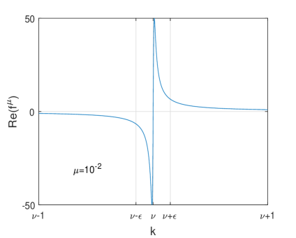
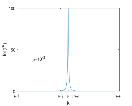
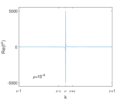
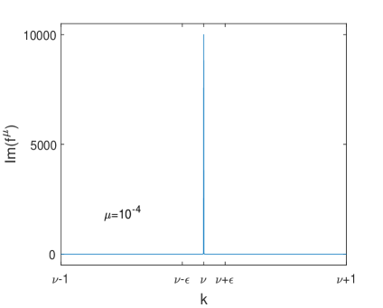
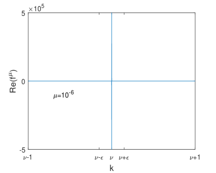
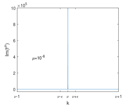
Figure 3: The analytical behaviour of the smooth integrand $f^{\mu}=\frac{1}{k-\nu-\mathrm{i}\mu}$ for $\nu=3$ with respect to $0<\mu\ll\epsilon\ll 1$.

3 Evaluation of the body wave motion problem

Now we consider the body oscillating in the fluid domain $D$. For a field point $\bm{q}=(x,y,z)\in D$, the velocity potential $\phi=\phi(\bm{q})$ has been expressed as a solution of the boundary integral equation (1). When the field point tends to the body boundary $S$, Eq. (1) reduces to the boundary integral equation

$$\phi(\bm{q})+\frac{1}{4\pi}\lim_{\bm{q}^{\prime}\in D,\bm{q}^{\prime}\to\bm{q}}\int_{S}\phi(\bm{p})\bm{n}\cdot\nabla G(\bm{q}^{\prime},\bm{p})\mathrm{d}S_{\bm{p}}=\frac{1}{4\pi}\int_{S}G(\bm{q},\bm{p})\bm{n}\cdot\nabla\phi(\bm{p})\mathrm{d}S_{\bm{p}}$$ (35)

for $\bm{q}\in S$.

Following the discretisation scheme of [20], the boundary integral equation (35) is now evaluated by the approximation expansions (28) and (33). The Hess-Smith Rankine formulation [20, 40, 41, 42] is employed to calculate the panel integral of the Rankine source potential and its normal derivative. To do so, the two-dimensional body surface $S$ is approximated by a set of mesh grid points $\bm{p}_{i,j}$ with $i=1,...,N+1$ and $j=1,...,M+1$ for suitable integers $N$ and $M$. A single $\mathit{panel}_{i,j}$ associated with a centre panel point $\bm{q}_{i,j}$ and a panel normal vector $\bm{n}_{i,j}$ pointing into the fluid domain is determined by the four vertices $\bm{p}_{i,j},\,\bm{p}_{i,j+1},\,\bm{p}_{i+1,j+1}$ and $\bm{p}_{i+1,j}.$

The boundary integral equation (35) is approximated in the form of the algebraic equation system, for $I=1,...,N$ and $J=1,...,M,$

$$\sum_{i=1}^{N}\sum_{j=1}^{M}\left(\delta_{I,J,i,j}+\mathcal{A}_{I,J,i,j}\right)\phi(\bm{q}_{i,j})=\sum_{i=1}^{N}\sum_{j=1}^{M}\bm{n}_{i,j}\cdot\nabla\phi(\bm{q}_{i,j})\mathcal{B}_{I,J,i,j}\,$$ (36)

for the Kronecker delta function $\delta$ with $\delta_{I,J,i,j}=1$ whenever $I=i$ and $J=j$. The influence coefficients of (36) are evaluated as

$$\mathcal{A}_{I,J,i,j}= -\lim_{\bm{q}\in D,\bm{q}\to\bm{q}_{{}_{I,J}}}\frac{1}{4\pi}\int_{\mathit{panel}_{i,j}}\,\bm{n}_{i,j}\cdot\nabla\frac{1}{|\bm{q}-\bm{p}|}\mathrm{d}S_{\bm{p}}$$

$$-\frac{1}{4\pi}\!\!\int_{\mathit{panel}_{i,j}}\!\!\!\!\!\!\!\bm{n}_{i,j}\!\cdot\!\nabla\frac{1}{|\bm{q}_{{}_{I,J}}-\bar{\bm{p}}|}dS_{\bm{p}}-\frac{|\mathit{panel}_{i,j}|}{4\pi}\bm{n}_{i,j}\!\cdot\!\nabla K(\bm{q}_{{}_{{}_{I,J}}},\bm{q}_{i,j}),$$ (37)

$$\mathcal{B}_{I,J,i,j} =-\int_{\mathit{panel}_{i,j}}\frac{\frac{1}{|\bm{q}_{{}_{I,J}}\!-\!\bm{p}|}+\frac{1}{|\bm{q}_{{}_{I,J}}\!-\!\bar{\bm{p}}|}}{4\pi}\mathrm{d}S_{\bm{p}}\!-\!\frac{|\mathit{panel}_{i,j}|}{4\pi}K(\bm{q}_{{}_{I,J}},\bm{q}_{i,j}).$$ (38)

Here $|\mathit{panel}_{i,j}|$ denotes the area of $\mathit{panel}_{i,j}$.

The evaluation of the panel integrals of (37) and (38) involving the Rankine source potential $\frac{1}{|\bm{q}_{{}_{I,J}}-\bm{p}|}$ and its image $\frac{1}{|\bm{q}_{{}_{I,J}}-\bar{\bm{p}}|}$ is obtained by the Hess-Smith quadrilateral integral method and has been detailed in [20].

Thus the algebraic equation (36) together with the boundary oscillation condition (5) can be solved from the Gaussian elimination scheme for the determination of the unknown $\phi(\bm{q}_{i,j})$.

4 Numerical results

For the validation of the numerical approximation scheme, selected numerical results with respect to the body wave motion problem (3)-(5) are displayed. Comparisons with the benchmark data given by Wang [16] and Hulme [14] will be presented with respect a submerged sphere and a floating hemisphere respectively. Let $r$ be the radius of the sphere or the hemisphere. The submergence of the sphere is defined by the parameter $h$, which measures the vertical distance between the calm water surface $z=0$ and the centre of the sphere. The mesh grid points are given by the spherical coordinates

$$\bm{p}_{i,j}=(r\sin\tau_{i}\cos\kappa_{j},\,r\sin\tau_{i}\sin\kappa_{j},\,-h+r\cos\tau_{i}),$$

for $i=1,...,N+1$ and $j=1,...,M+1$. Here $-\pi\leq\kappa_{j}<\pi$, $0\leq\tau_{i}\leq\pi$ for the submerged sphere and $\pi/2\leq\tau_{i}\leq\pi$ for the floating hemisphere.

As illustrated in Figure 2, the parameter $\mu=10^{-4}$ is selected. The numerical computation is stable with respect to the choice of the parameters $k_{\mathrm{m}ax}$, $N_{k}$, $N$ and $M$. For the comparison purpose with respect to added mass and damping coefficients, they are selected as $k_{\mathrm{m}ax}\leq 14$, $N_{k}\leq 1100$, $N\leq 20$ and $M\leq 40$. Here we only provide upper bounds of the parameter. Actually, the bounds can be lowered and are dependent on individual motions. For example, for the heave motion of the sphere submerged at the water depth $h/r=1.5$, satisfactory numerical results can be produced by taking $k_{\mathrm{m}ax}=6$, $N_{k}=500$, $N=12$ and $M=14$. However, for the floating hemisphere, smaller mesh panels and larger truncation integral interval $[0,k_{\mathrm{m}ax}]$ for the regular wave integral are required as the stability of the wave integral is reduced around the free surface $z=0$.

For the numerical velocity potential solution $\phi=\phi_{\alpha}$ ($\alpha=1,2,3$) of the boundary value problem (5) and (36), the linear hydrodynamic pressure is expressed as

$$p_{\alpha}=-\rho\frac{\partial\Phi_{\alpha}}{\partial t}=\omega\rho\mathrm{Re}\left(\mathrm{i}\phi_{\alpha}\mathrm{e}^{-\mathrm{i}\omega t}\right)$$

for $\rho$ the fluid density. This defines the hydrodynamic wave force exerted on the average wetted body surface $S$:

$$F_{\alpha,\alpha}=\int_{S}p_{\alpha}n_{\alpha}dS$$

and the non-dimensional added mass and damping coefficients $A_{\alpha,\alpha}$ and $B_{\alpha,\alpha}$:

$$A_{\alpha,\alpha}+\mathrm{i}B_{\alpha,\alpha}=\frac{1}{\omega V}\int_{S}\mathrm{i}\phi_{\alpha}n_{\alpha}\mathrm{d}S=\frac{1}{\omega V}\sum_{i=1}^{N}\sum_{j=1}^{M}\mathrm{i}\phi_{\alpha}(\bm{q}_{i,j})n_{\alpha}(\bm{q}_{i,j})|\mathit{panel}_{i,j}|.$$ (39)

Here $V$ is the volume of the moving body with the wetted body surface $S$. Especially, $V=\frac{4}{3}\pi r^{3}$ for the submerged sphere and $V=\frac{2}{3}\pi r^{3}$ for the floating hemisphere.

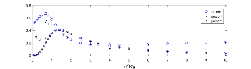
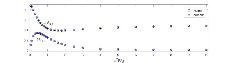
Figure 4: Added mass and damping coefficients produced by the present method and the semi-analytic solution data of Hulme [14] for the floating hemisphere in heaving or surging motions.

For the wave motion of the floating hemisphere, present method results of $A_{\alpha,\alpha}$ and $B_{\alpha,\alpha}$ for surging motion ($\alpha=1$) and heaving motion ($\alpha=3$) are displayed in Figure 4, which shows the existence of irregular frequency for $\omega^{2}r/g$ around $4$ in a high frequency, the same phenomenon shown in [20]. As is well known [1, 2, 44, 45] that the combination of panel method and free surface Green function gives rise to irregular frequencies in a high frequency range when a floating body undergoes oscillatory motions. Various methods exist (see, for example, [2, 3, 44, 46]) to remove non-physical irregular frequencies. When $\omega^{2}r/g$ is away from the irregular frequency point, Figure 4 presents excellent agreement between numerical solution and the semi-analytic solution of the celebrated work of Hulme [14] for a heaving hemisphere.

For a fully submerged body of a radius $r$ at a submergence depth $h$, the irregular frequency phenomenon does not occur due to stability improvement of the free surface Green function, since the individual incident wave potentials $\mathrm{e}^{k_{j}(z+\zeta)}J_{0}(k_{j}R)$ and $\mathrm{e}^{k_{j}(z+\zeta)}J_{1}(k_{j}R)$ in (28)-(30) are controlled by the exponentially decay function $\mathrm{e}^{k_{j}(z+\zeta)}$. Numerical solutions of heaving and surging motions with respect to the submerged sphere are presented in Figure 5 showing that the present method solution agrees well with the semi-analytic solution of Wang [16].

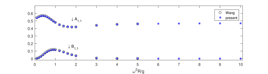
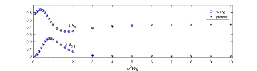
Figure 5: Added mass and damping coefficients produced by the present method and the semi-analytic solution data of Wang [16] for the heaving or surging sphere submerged at the water depth of $h/r=1.5$.

5 Discussion and conclusion

The free surface Green function represents a pulsating free surface source potential, which is the sum of the Rankine simple Green function, its image with regarding to the average free water surface and a singular wave integral. Thence the evaluation of the Green function means that of the singular wave integral.

With the rapid development of computing capacity, numerical computation of a linear hydrodynamic problem is no longer time consuming. However, the Green function evaluation due to the presence of an singular wave integral is still known to be troublesome and sophisticated mathematical treatments are supposed to be employed to attack the singularity [21, 22, 23, 24, 25]. Therefore, the purpose of the present investigation is not for reducing the numerical simulation time in solving a linear hydrodynamics problem, but to simplify the accessibility to coding a body wave motion flow.

The problematic singular pole $k=\nu$ of singular wave integral (2) is removable by using the continuous elementary function $\frac{1}{k-\nu-\mathrm{i}\mu}$ with $0<\mu\ll 1$ in place of the unbounded function $\frac{1}{k-\nu}$ along the integration line $k>0$. Although the continuous function reaches high peaks $\pm\frac{1}{2\mu}$ for its real part and $\frac{1}{\mu}$ for its imaginary part in a vicinity of the wave number $k=\nu$, the combination of two real integration areas with respect to positive and negative peaks $\pm\frac{1}{2\mu}$ around $k=\nu$ is zero, while the imaginary integration area with respect to the peak $\frac{1}{\mu}$ remains unchanged for small $\mu$ (see Figure 3). That is, the integration can be calculated in the straightforward and simple way:

$$\int^{\nu+\epsilon}_{\nu-\epsilon}\frac{f(k)dk}{k-\nu-\mathrm{i}\mu}=f(\nu)\int^{\nu+\epsilon}_{\nu-\epsilon}\frac{dk}{k-\nu-\mathrm{i}\mu}=f(\nu)\ln\frac{\epsilon-\mathrm{i}\mu}{-\epsilon-\mathrm{i}\mu}=\mathrm{i}\pi f(\nu)$$ (40)

for a continuous function $f$ and parameters $0<\mu\ll\epsilon\ll 1$. Thus there is no special treatment required with respect to the wave number $k=\nu$.

The author’s previous study [20] shows that the direct integration of the wave integral to obtain the approximations (8)-(9). In the present investigation, the expansions (8)-(9) are simplified to the form (28)-(33). The approximation stability of the gradient $\nabla K$ is significantly improved as the stability of the expansion for $\nabla K$ is the same with that for $K$ in (28)-(33).

As a sample application, this scheme is employed to compute numerically the wave motion problems of a floating sphere and a submerged sphere respectively in harmonic waves in order to compare with the benchmark data of [14, 16]. Figures 4 and 5 indicate the sufficient accuracy to compute linear wave loads in practice.

The efficiency of the present scheme is twofold. Firstly, we use the single integrals $K^{\mu}$, $\partial_{R}K^{\mu}$ and $\partial_{z}K^{\mu}$ rather the double integrals in [20]. Secondary, the partial derivative $\partial_{z}K^{\mu}$ in (23) is in a linear form of $K^{\mu}$ in (16) and, moreover, the partial derivative $\partial_{R}K^{\mu}$ in (22) is also a linear form of $K^{\mu}$ if $J_{1}$ is replaced by $J_{0}$. Thus the numerical computation of the gradient $\nabla K^{\mu}$ essentially becomes that of $K^{\mu}$.

Acknowledgement. This work is supported by NSFC of China (11571240).

References

- [1] W. Frank, Oscillation of cylinders in or below the free surface of deep fluids, Rep. 2375, Naval Ship Res. Dev. Center, Bethesda, MD, 1967.
- [2] C.H. Lee, P.D. Sclavounos, Removing the irregular frequencies from integral equations in wave-body interactions, J. Fluid Mech. 207 (1989) 393-418.
- [3] C.H. Lee, J.N. Newman, X. Zhu, An extended boundary integral equation method for the removal of irregular frequency effects, Int. J. Numer. Meth. Fluids 23 (1996) 637-660.
- [4] C.H. Lee, J.N. Newman, Computation of wave effects using the panel method, In: S.K. Chakrabart (Ed.), Numerical Models in Fluid-Structure Interaction, WIT Press, Southampton, 2004.
- [5] H. Liang, H. Wu, F. Noblesse, Validation of a global approximation to the Green function of diffraction radiation in deep water, Appl. Ocean Res. 74 (2018) 80-86.
- [6] C.W. Dawson, A practical computer method for solving ship wave problems, In Proceedings of 2nd International Conference on Numerical Ship Hydrodynamics, University of California, Berkeley, 30-38, 1977.
- [7] R.W. Yeung, Added mass and damping of a vertical cylinder in finite depth waters, Appl. Ocean Res. 3 (1981) 119-133.
- [8] Y. Cao, W. Schultz, R. Beck, Three-dimensional desingularized boundary integral methods for potential problems, Int. J. Numer. Meth. Fluids 12 (1991) 785-803.
- [9] D.A. Mantzaris, A Rankine Panel Method as a Tool for the Hydrodynamic Design of Complex Marine Vehicles, PhD thesis, MIT, 1998.
- [10] A. Feng, Z.M. Chen, W.G. Price, A Rankine source computation for three dimensional wave-body interactions adopting a nonlinear body boundary condition, Appl. Ocean Res. 47 (2014), 313-321.
- [11] A. Feng, Z.M. Chen, W.G. Price, A continuous desingularized source distribution method describing wave-body interactions of a large amplitude oscillatory body, J. Offshore Mech. Arctic Eng. 137 (2015), 021302
- [12] F. Ursell, On the heaving motion of a circular cylinder on the surface of a fluid, Quart. J. Mech Appl. Math. 2 (1949) 218-231.
- [13] T. Havelock, Waves due to a floating hemi-sphere making periodic heaving oscillations, Proc. R. Soc. Lond. A 231 (1955) 1-7.
- [14] A. Hulme, The wave forces acting on a floating hemisphere undergoing forced periodic oscillations, J. Fluid Mech. 121 (1982) 443-463.
- [15] C. Farell, On the wave resistance of a submerged spheroid, J. Ship Res. 17 (1973) 1-11.
- [16] S. Wang, Motions of a spherical submarine in waves, Ocean Eng. 13 (1986) 249-271.
- [17] G.X. Wu, R. Eatock Taylor, The exciting force on a submerged spheroid in regular waves, J. Fluid Mech. 182 (1987) 411-426.
- [18] I.K. Chatjigeorgiou, The analytic solution for hydrodynamic diffraction by submerged prolate spheroids in infinite water depth, J. Eng. Math. 81 (2013) 47-65.
- [19] J.V. Wehausen, E.V. Laitone, Surface waves, In: S. Flugge, C. Truesdell (Eds.), Fluid Dynamics III in Handbuch der Physik 9, Springer, Berlin, 446-778, 1960.
- [20] Z.M. Chen, Regular wave integral approach to numerical simulation of radiation and diffraction of surface waves, Wave Motion 52 (2015) 171-182.
- [21] J.N. Newman, Algorithms for the free-surface Green functions, J. Eng. Math. 19 (1985) 57-67.
- [22] F. Noblesse, The Green function in the theory of radiation and diffraction of regular water waves by a body, J. Eng. Math. 16 (1982) 137-169.
- [23] J.L. Hess, D.C. Wilcox, Progress in the solution of the problem of a three-dimensional body oscillating in the presence of a free surface - Final technical report, McDonnell Douglas Company Rep. DAC 67647, 1969.
- [24] M.A. Peter, M.H. Meylan, The eigenfunction expansion of the infinite depth free surface Green function in three dimensions, Wave Motion 40 (2004) 1-11.
- [25] H. Wu, C. Zhang, Y. Zhu, W. Li, D. Wan, F. Noblesse, A global approximation to the Green function for diffraction radiation of water waves, European J. Mech. B Fluids 65 (2017) 54-64.
- [26] T.H. Havelock, Wave resistance, Proc. R. Soc. Lond. A 118 (1928) 24-33.
- [27] T.H. Havelock, The theory of wave resistance. Proc. R. Soc. Lond. A 138 (1932) 339-348.
- [28] F. Noblesse, D. Hendrix, On the theory of potential flow about a ship advancing in waves, J. Ship Res. 36 (1992) 17-29.
- [29] F. Noblesse, X.B. Chen, Decomposition of free-surface effects into wave and near-field components, Ship Tech. Res. 42 (1995) 167-185.
- [30] F. Noblesse, C. Yang, Fourier representation of near-field free-surface flows, Ship Tech. Res. 43 (1996) 19-37.
- [31] J.N. Newman, Evaluation of the Wave-Resistance Green function: Part 1–The double integral. J. Ship Res. 31 (1987) 79-90.
- [32] Z.M. Chen, A vortex based panel method for potential flow simulation around a hydrofoil, J. Fluids Struct. 28 (2012) 378-391.
- [33] Z.M. Chen, W.G. Price, Supercritical regimes of liquid-metal fluid motions in electromagnetic fields: wall-bounded flows, Proc. R. Soc. A 458 (2002) 2735-2757.
- [34] Z.M. Chen, W.G. Price, Secondary fluid flows driven electromagnetically in a two-dimensional extended duct, Proc. R. Soc. A 461 (2005) 1659-1683.
- [35] R. Brard, The representation of a given ship form by singularity distributions when the boundary condition on the free surface is linearized, J. Ship Res. 16 (1971) 79-92.
- [36] P. Guevel, P. Vaussy, J.M. Kobus, The distribution of singularities kinematically equivalent to a moving hull in the presence of a free surface, Int. Shipbuild Prog. 21 (1974) 311-324.
- [37] F. Noblesse, F. Huang, C. Yang, The Neumann-Michell theory of ship waves, J. Eng. Math. 79 (2013) 51-71.
- [38] F. Huang, A practical Computational Method for Steady Flow About a Ship, PhD thesis, George Mason University, 2013.
- [39] M. Abramowitz, I. A. Stegun, Handbook of Mathematical Functions with Formulas, Graphs, and Mathematical Tables, Dover, New York, 1965.
- [40] A.J. Hess, A.M.O. Smith, Calculation of non-lifting potential flow about arbitrary three-dimensional bodies, Report No. E.S. 40622, Douglas Aircraft Co., Inc. Aircraft Division, Long Beach, California, 1962.
- [41] A.J. Hess, A.M.O. Smith, Calculation of potential flow about arbitrary bodies, Prog. Aerospace Sci. 8 (1966) 1-138.
- [42] J.N. Newman, Distributions of sources and normal dipoles over a quadrilateral panel, J. Eng. Math. 20 (1986) 113-126.
- [43] T.H. Havelock, The theory of wave resistance, Proc. R. Soc. Lond. A 138 (1932) 339-348.
- [44] F. Ursell, Irregular frequencies and the motion of floating bodies, J. Fluid Mech. 105 (1981) 143-156.
- [45] F. John, On the motion of floating bodies II. Simple harmonic motions, Communs. Pure Appl. Math. 3 (1950) 45-101.
- [46] X. Zhu, C.H. Lee, Removing the irregular frequencies in wave-body interactions, The 9th International Workshop on Water Waves and Floating Bodies, Japan, 245-249, 1994.