On the Diversity of Uncoded OTFS Modulation in Doubly-Dispersive Channels

Abstract

Orthogonal time frequency space (OTFS) is a 2-dimensional (2D) modulation technique designed in the delay-Doppler domain. A key premise behind OTFS is the transformation of a time varying multipath channel into an almost non-fading 2D channel in delay-Doppler domain such that all symbols in a transmission frame experience the same channel gain. It has been suggested in the recent literature that OTFS can extract full diversity in the delay-Doppler domain, where full diversity refers to the number of multipath components separable in either the delay or Doppler dimension, but without a formal analysis. In this paper, we present a formal analysis of the diversity achieved by OTFS modulation along with supporting simulations. Specifically, we prove that the asymptotic diversity order of OTFS (as SNR $\rightarrow\infty$) is one. However, in the finite SNR regime, potential for a higher order diversity is witnessed before the diversity one regime takes over. Also, the diversity one regime is found to start at lower BER values for increased frame sizes. We also propose a phase rotation scheme for OTFS using transcendental numbers and show that OTFS with this proposed scheme extracts full diversity in the delay-Doppler domain.

Keywords – OTFS modulation, delay-Doppler domain, diversity order, phase rotation, MIMO-OTFS.

I Introduction

Future wireless communication systems are envisioned to support diverse requirements that include high mobility application scenarios such as high-speed train, vehicle-to-vehicle, and vehicle-to-infrastructure communications. The dynamic nature of wireless channels in such scenarios makes them doubly-dispersive, with multipath propagation effects causing time dispersion and Doppler shifts causing frequency dispersion [1]. Conventional multicarrier modulation techniques such as orthogonal frequency division multiplexing (OFDM) mitigate the effect of inter-symbol interference (ISI) caused due to time dispersion. However, the performance of OFDM systems depends significantly on the orthogonality among the subcarriers. Doppler shifts can destroy the orthogonality among the subcarriers, resulting in inter-carrier interference (ICI) which degrades performance [2].

Orthogonal time frequency space (OTFS) modulation is a recently proposed modulation scheme [3]-[7] that uses delay-Doppler domain for multiplexing the information symbols instead of time-frequency domain as in conventional modulation schemes. OTFS modulation uses transformations that spread information across the time-frequency plane. This spreading across the time-frequency plane converts a doubly-dispersive channel into an almost non-fading channel in the delay-Doppler domain. The relatively constant channel gain experienced by all the symbols in an OTFS transmission frame can greatly reduce the overhead on the channel estimation in a rapidly time varying channel. Another attractive feature of OTFS from an implementation viewpoint is that OTFS modulation can be architected over any multicarrier modulation (e.g., OFDM) by using additional pre-processing and post-processing blocks [5].

OTFS has been shown to achieve significantly better error performance compared to OFDM for vehicle speeds ranging from 30 km/h to 500 km/h in 4 GHz band [3]. It has also been shown to perform well in mmWave frequency bands [7]. Owing to the simplicity of implementation and robustness to Doppler spreads, several works on OTFS have started emerging in the recent literature [8]-[12]. OTFS systems using OFDM as the inner core have been considered in [8],[9]. In [10],[11], the robustness of OTFS modulation has been demonstrated in high Doppler fading channels, using low complexity signal detection techniques. While [10] proposed a message passing based algorithm for OTFS signal detection, [11] proposed a Markov Chain Monte Carlo based algorithm for detection and a pseudo-random noise (PN) pilot based scheme for channel estimation in the delay-Doppler domain. The above detection algorithms were devised using a system model based on the vectorized input-output relation for OTFS [10]. Signal detection and channel estimation for multiple-input multiple-output OTFS (MIMO-OTFS) have been considered in [12], where it has been shown that MIMO-OTFS offers significantly better performance compared to MIMO-OFDM. It has been highlighted in [3] that the OTFS modulation can be viewed as a generalization of TDMA and OFDM. Likewise, OTFS can also be interpreted as a generalization of other multicarrier modulation schemes such as filtered multitone [13] and generalized frequency division multiplexing (GFDM) [14]. Recently, it has been shown in [15] that OTFS can be implemented using a GFDM framework.

While recent papers on OTFS have demonstrated the performance superiority of OTFS over OFDM, a formal analysis and claim on the diversity order achieved by OTFS is yet to appear. It has been suggested in [4] that OTFS can achieve full diversity in the delay-Doppler domain, where full diversity refers to the number of clustered reflectors in the channel (in other words, the number of multipath components separable in either the delay or Doppler dimension). However, this suggestion has not been established through analysis or simulation. Filling this gap, our contribution in this paper provides a formal analysis of the diversity order achieved by OTFS in doubly-dispersive channels with supporting simulation results. The key findings and contributions in this work can be summarized as follows.

• We first derive the diversity order of OTFS in a single-input single-output (SISO) setting with maximum likelihood (ML) detection. It is shown that that the asymptotic diversity order of OTFS (as SNR $\rightarrow\infty$) is one. Though the asymptotic diversity order is one, potential for a higher order diversity is witnessed in the finite SNR regime before the diversity one regime takes over. Also, it is observed that the diversity one regime starts at lower BER values for increased frame sizes. A lower bound on the BER computed by summing up the pairwise error probabilities corresponding to all pairs of data matrices whose difference matrices have rank one provides an analytical support for this observation.

• Next, in an attempt to extract full diversity in the asymptotic regime, we propose a phase rotation scheme for OTFS using transcendental numbers. It is shown that OTFS with this proposed scheme extracts the full diversity in the delay-Doppler domain.

• Finally, we extend the diversity analysis to MIMO-OTFS and show that the asymptotic diversity order is equal to the number of receive antennas. We also extend the phase rotation scheme to MIMO-OTFS system to extract full diversity in the delay-Doppler domain.

The rest of the paper is organized as follows. The OTFS modulation scheme is presented in Sec. II. The diversity analysis of OTFS in SISO setting and corresponding simulation results are presented in Sec. III. The proposed phase rotation scheme that achieves full diversity is presented in Sec. IV. The MIMO-OTFS system, its asymptotic diversity order, and phase rotation scheme are presented in Sec. V. Conclusions are presented in Sec. VI.

II OTFS modulation

In this section, we describe OTFS modulation designed in the delay-Doppler domain. We first introduce the delay-Doppler representation and the associated transforms and then present the mathematical description of the OTFS modulation.

II-A Delay-Doppler representation and OTFS modulation

Fundamentally, a signal can be represented either as a function of time, or as a function of frequency, or as a quasi-periodic function of delay and Doppler [5]. These three representations are interchangeable by means of the canonical transforms, as depicted in Fig. 1. The nodes of the triangle represent the three ways of representing a signal and the edges represent the canonical transformation used for the conversion between them. The conversion between the time and frequency representations is through the Fourier transform, and the conversion of the delay-Doppler representation to the time and frequency representations is through the Zak transforms $Z_{t}$ and $Z_{f}$, respectively. It is important to note that the composition of any pair of transforms is equal to the remaining one. For example, the Fourier transform is a composition of two Zak transforms ($\mbox{FT}=Z_{t}\circ Z_{f}^{-1}$). The signals in the delay-Doppler domain can be viewed as functions $\phi(\tau,\nu)$ on a two-dimensional delay-Doppler plane whose points are parametrized by $\tau$ and $\nu$. This representation is a quasi-periodic representation and has an associated delay period $\tau_{r}$ and a Doppler period $\nu_{r}$, such that $\tau_{r}\nu_{r}=1$. The delay-Doppler representation can be converted to time and frequency representations by Zak transforms $Z_{t}$ and $Z_{f}$, respectively, given by [5]

$$Z_{t}(\phi)=\int_{0}^{\nu_{r}}e^{j2\pi t\nu}\phi(t,\nu)\mathrm{d}\nu,\ \ Z_{f}(\phi)=\int_{0}^{\tau_{r}}e^{-j2\pi\tau f}\phi(\tau,f)\mathrm{d}\tau.$$ (1)

Figure 1: The fundamental transform triangle.

A fundamental feature of OTFS modulation that distinguishes it from other time-frequency (TF) modulation schemes is the use of delay-Doppler domain for multiplexing the modulation symbols. These symbols in the delay-Doppler domain can be converted into time domain using the Zak transform $Z_{t}$. The transformation that uses a single Zak transform to convert a signal in delay-Doppler domain to a signal in time domain can also be carried out in two steps. That is, the signal in the delay-Doppler domain is first transformed to time-frequency domain, and the resulting time-frequency signal is converted to a time domain signal using a second transformation. As a consequence of this two step transformation, OTFS modulation can be implemented using simple pre- and post-processing steps over any multicarrier modulation scheme such as OFDM. The series of transformations involved in OTFS modulation transforms a time varying multipath channel into a slowly varying channel in the delay-Doppler domain. The complex baseband channel response in the delay-Doppler domain is denoted by $h(\tau,\nu)$, where $\tau$ and $\nu$ are the delay and Doppler variables, respectively. With this representation, the received signal $y(t)$ due to a transmit signal $x(t)$ is given by

$$y(t)=\int_{\nu}\int_{\tau}h(\tau,\nu)x(t-\tau)e^{j2\pi\nu(t-\tau)}\mathrm{d}\tau\mathrm{d}\nu.$$ (2)

The channel coefficients in this representation correspond to the group of reflectors associated with a particular delay depending on reflectors’ relative distance and Doppler value depending on its relative velocity. Since the velocity and the relative distance remain roughly the same for a relatively longer duration, the delay-Doppler channel coefficients are time invariant for a larger observation time as compared to that in time-frequency representation [6]. Also, the delay-Doppler representation of the channel impulse response yields a sparse representation of the channel, thus requiring only fewer channel parameters to be estimated. With this, we now proceed to the description of the OTFS modulation scheme architected using pre- and post-processing operations over a multicarrier modulation.

Figure 2: OTFS modulation scheme.

The block diagram of the OTFS modulation scheme is shown in Fig. 2. The inner box in the block diagram is the familiar multicarrier TF modulation and the outer box with pre- and post-processor is the OTFS modulator that operates in the delay-Doppler domain. At the transmitter, the information symbols (e.g., QAM symbols) denoted by $x[k,l]$ residing in delay-Doppler domain are mapped to the TF signal $X[n,m]$ through the 2D inverse symplectic finite Fourier transform (ISFFT) and windowing. Subsequently, this TF signal is transformed into a time domain signal $x(t)$ through Heisenberg transform for transmission. At the receiver, the received signal $y(t)$ is transformed back to a TF domain signal $Y[n,m]$ through Wigner transform (inverse Heisenberg transform). The TF signal $Y[n,m]$ thus obtained is mapped to the delay-Doppler domain signal $y[k,l]$ using the symplectic finite Fourier transform (SFFT) for demodulation. In the subsequent subsections, we describe the TF modulation and the OTFS modulation in detail.

II-B Time-frequency modulation

• The time-frequency plane is sampled at intervals $T$ and $\Delta f$, respectively, to obtain a 2D lattice or grid $\Lambda$, which can be defined as $\Lambda=\{(nT,m\Delta f),n=0,\cdots,N-1,m=0,\cdots,M-1\}$.

• The signal in TF domain $X[n,m]$, $n=0,\cdots,N-1$, $m=0,\cdots,M-1$ is transmitted in a given packet burst, which has duration $NT$ and occupies a bandwidth of $M\Delta f$.

• Let $g_{tx}(t)$ and $g_{rx}(t)$ denote the transmit and receive pulses, respectively. We assume $g_{tx}(t)$, $g_{rx}(t)$ to be ideal pulses satisfying the bi-orthogonality property with respect to translations by integer multiples of time $T$ and frequency $\Delta f$, i.e.,

  $$\int e^{-j2\pi m\Delta f(t-nT)}g^{*}_{rx}(t-nT)g_{tx}(t)dt=\delta(m)\delta(n).$$ (3)

  The bi-orthogonality property of the pulse shapes ensures that the cross-symbol interference is eliminated in the symbol reception. Although ideal pulses cannot be realized in practice, given the constraint imposed by the uncertainty principle, they can be approximated by the pulses whose support is highly concentrated in time and frequency [10]. Design of pulses concentrated in time and frequency to minimize the cross-symbol interference has been discussed in [16],[17].

• TF modulation: The signal in TF domain $X[n,m]$ is transformed to the time domain signal $x(t)$ through the Heisenberg transform, given by

  $$x(t)=\sum_{n=0}^{N-1}\sum_{m=0}^{M-1}X[n,m]g_{tx}(t-nT)e^{j2\pi m\Delta f(t-nT)}.$$ (4)

• TF demodulation: At the receiver, the sufficient statistic for symbol detection is obtained by matched filtering the received signal with the receive pulse $g_{rx}(t)$. This requires the computation of the cross-ambiguity function $A_{g_{rx},y}(\tau,\nu)$, given by

  $$A_{g_{rx},y}(\tau,\nu)=\int g_{rx}^{*}(t-\tau)y(t)e^{-j2\pi\nu(t-\tau)}\mathrm{d}t.$$ (5)

  Sampling this function on the lattice $\Lambda$ yields the matched filter output, given by

  $$Y[n,m]=A_{g_{rx},y}(\tau,\nu)|_{\tau=nT,\nu=m\Delta f}.$$ (6)

  Equation (6) is called the Wigner transform, which can be looked at as the inverse of the Heisenberg transform. A detailed discussion on Heisenberg and Wigner representations and its applications in communication theory has been presented in [18],[19].

• If $h(\tau,\nu)$ has finite support bounded by $(\tau_{\mbox{\scriptsize{max}}},\nu_{\mbox{\scriptsize{max}}})$ and if $A_{g_{rx}g_{tx}}(\tau,\nu)=0$ for $\tau\in(nT-\tau_{\mbox{\scriptsize{max}}},nT+\tau_{\mbox{\scriptsize{max}}})$, $\nu\in(m\Delta f-\nu_{\mbox{\scriptsize{max}}},m\Delta f+\nu_{\mbox{\scriptsize{max}}})$, $\forall n,m$ except for $n=0,m=0$ where $A_{g_{rx}g_{tx}}(\tau,\nu)=1$, the relation between $Y[n,m]$ and $X[n,m]$ for TF modulation can be derived as [4]

  $$Y[n,m]=H[n,m]X[n,m]+V[n,m],$$ (7)

  where $V[n,m]$ is the noise at the output of the matched filter and $H[n,m]$ is given by

  $$H[n,m]=\int_{\tau}\int_{\nu}h(\tau,\nu)e^{j2\pi\nu nT}e^{-j2\pi(\nu+m\Delta f)\tau}\mathrm{d}\nu\mathrm{d}\tau.$$ (8)

From (7), note that $X[n,m]$ is not affected by cross-symbol interference either in time or in frequency. In the absence of noise, the received symbol $X[n,m]$ is same as the transmitted symbol except for the complex scale factor $H[n,m]$. Note that the complex scale factor $H[n,m]$ is a weighted superposition of Fourier exponential functions. This relation can be formally expressed via a two dimensional transform called the symplectic Fourier transform.

II-C OTFS modulation

• Let $X_{p}[n,m]$ denote the periodized version of $X[n,m]$ with period $(N,M)$. The SFFT of $X_{p}[n,m]$ is defined as

  $$x_{p}[k,l]=\sum_{n=0}^{N-1}\sum_{m=0}^{M-1}X_{p}[n,m]e^{-j2\pi({nk\over N}-{ml\over M})},$$ (9)

  and ISFFT of $x_{p}[k,l]=SFFT^{-1}(x_{p}[k,l])$ is defined as

  $$X_{p}[n,m]={1\over MN}\sum_{k=0}^{N-1}\sum_{l=0}^{M-1}x_{p}[k,l]e^{j2\pi({nk\over N}-{ml\over M})}.$$ (10)

• OTFS transform: The information symbols in the delay-Doppler domain $x[k,l]$ are mapped to TF domain symbols $X[n,m]$ as follows:

  $$X[n,m]=W_{tx}[n,m]SFFT^{-1}(x_{p}[k,l]),$$ (11)

  where $W_{tx}[n,m]$ is the transmit windowing square summable function.

• $X[n,m]$ thus obtained is in TF domain and is TF modulated as described in the previous subsection for transmission through the channel.

• OTFS demodulation: The received signal $y(t)$ is transformed into $Y[n,m]$ using Wigner filter as in (6). A receive window $W_{rx}[n,m]$ is applied to $Y[n,m]$ to obtain $Y_{W}[n,m]=W_{rx}[n,m]Y[n,m]$. This is periodized to obtain $Y_{p}[n,m]$ with period $(N,M)$, given by

  $$Y_{p}[n,m]=\sum_{k,l=-\infty}^{\infty}Y_{W}[n-kN,m-lM].$$ (12)

• The symplectic finite Fourier transform is then applied to $Y_{p}[n,m]$ to convert it from TF domain back to delay-Doppler domain to obtain $y_{p}[k,l]$ as

  $$y_{p}[k,l]=SFFT(Y_{p}[n,m]).$$ (13)

  The output sequence of demodulated symbols is obtained as $y[k,l]=y_{p}[k,l]$ for $k=0,1,\cdots,N-1$ and $l=0,1,\cdots,M-1$.
  Note: Periodization here can be understood by taking the analogy of the discrete time Fourier transform (DTFT). The DTFT of a discrete time signal is a continuous and periodic function of frequency. Sampling the spectrum in the frequency domain periodizes the signal in the time domain. Analogously, the discrete symplectic Fourier transform (DSFT) of a sequence is continuous and periodic [20]. Sampling the DSFT of a sequence in the delay-Doppler domain periodizes the signal in the time-frequency domain.

Using the equations (4)-(13), the input-output relation in OTFS can be derived as [3]

$$y[k,l]={1\over MN}\sum_{l^{\prime}=0}^{M-1}\sum_{k^{\prime}=0}^{N-1}x[k^{\prime},l^{\prime}]h_{w}\left({k-k^{\prime}\over NT},{l-l^{\prime}\over M\Delta f}\right)+v[k,l],$$ (14)

where

$$h_{w}\left({k-k^{\prime}\over NT},{l-l^{\prime}\over M\Delta f}\right)=h_{w}(\nu,\tau)|_{\nu={k-k^{\prime}\over NT},\tau={l-l^{\prime}\over M\Delta f}},$$ (15)

where $h_{w}(\nu,\tau)$ is the circular convolution of the channel response with a windowing function $w(\nu,\tau)$, given by

$$h_{w}(\nu,\tau)=\int_{\nu^{\prime}}\int_{\tau^{\prime}}h(\tau^{\prime},\nu^{\prime})w(\nu-\nu^{\prime},\tau-\tau^{\prime})e^{-j2\pi\tau\nu}\mathrm{d}\tau^{\prime}\mathrm{d}\nu^{\prime},$$ (16)

and $w(\nu,\tau)$ is the discrete symplectic Fourier transform (DSFT) of the time-frequency window, defined as

$$w(\nu,\tau)=\sum_{m=0}^{M-1}\sum_{n=0}^{N-1}W_{tx}[n,m]W_{rx}[n,m]e^{-j2\pi(\nu nT-\tau m\Delta f)}.$$ (17)

Note that the circular convolution in (16) does not involve any cyclic prefixing. Circular convolution here arises naturally from the OTFS pre- and post-processing (ISFFT and SFFT) operations (from Theorem 2 of [4]).

II-D Vectorized formulation of the input-output relation

Consider a channel with $P$ paths, resulting from $P$ clusters of reflectors, where each reflector is associated with a delay and a Doppler, which can be represented in delay-Doppler domain as

$$h(\tau,\nu)=\sum_{i=1}^{P}h_{i}\delta(\tau-\tau_{i})\delta(\nu-\nu_{i}),$$ (18)

where $h_{i}$, $\tau_{i}$, $\nu_{i}$ represent the channel gain, delay, and Doppler shift associated with $i$th cluster, respectively. We define $\tau_{i}\triangleq\frac{\alpha_{i}+a_{i}}{M\Delta f}$ and $\nu_{i}\triangleq\frac{\beta_{i}+b_{i}}{NT}$, where $\alpha_{i}$, $\beta_{i}$ are integers and $a_{i},b_{i}$ are real, where $-\frac{1}{2}<a_{i},b_{i}\leq\frac{1}{2}$. We refer to $a_{i}$ and $b_{i}$ as the fractional parts of delay $\tau_{i}$ and Doppler $\nu_{i}$, respectively. The fractional parts $a_{i}$ and $b_{i}$ can be neglected if $M$ and $N$ are large, and hence the delay resolution $1/M\Delta f$ and the Doppler resolution $1/NT$ are sufficiently small to approximate the path delays and Doppler shifts to the nearest integer sampling points [21]. We initially assume the fractional parts $a_{i}$s and $b_{i}$s to be zero and carry out the diversity analysis of OTFS in Sec. III. We extend the diversity analysis for non-zero fractional delays and Dopplers (i.e., $a_{i},b_{i}\neq 0$) in Appendix A. Assuming $\tau_{i}=\frac{\alpha_{i}}{M\Delta f}$ and $\nu_{i}=\frac{\beta_{i}}{NT}$ and assuming the transmit and receive window function $W_{tx}[n,m]$ and $W_{rx}[n,m]$ to be rectangular, the input-output relation for the channel in (18) can be derived as [10]

$$y[k,l]=\sum_{i=1}^{P}h_{i}^{\prime}x[(k-\beta_{i})_{N},(l-\alpha_{i})_{M}]+v[k,l].$$ (19)

The $h_{i}^{\prime}$s are given by

$$h_{i}^{\prime}=h_{i}e^{-j2\pi\nu_{i}\tau_{i}},$$ (20)

where $h_{i}$s are assumed to be i.i.d and distributed as $\mathcal{CN}(0,1/P)$ (assuming uniform scattering profile). The input-output relation in (19) can be vectorized as [10]

$$\mathbf{y}=\mathbf{Hx}+\mathbf{v},$$ (21)

where $\mathbf{x},\mathbf{y},\mathbf{v}\in\mathbb{C}^{MN\times 1}$, $\mathbf{H}\in\mathbb{C}^{MN\times MN}$, the $(k+Nl)$th element of $\mathbf{x}$, $x_{k+Nl}=x[k,l]$, $k=0,\cdots,N-1,\ l=0,\cdots,M-1$, and $x[k,l]\in\mathbb{A}$, where $\mathbb{A}$ is the modulation alphabet (e.g., QAM / PSK). Likewise, $y_{k+Nl}=y[k,l]$ and $v_{k+Nl}=v[k,l]$, $k=0,\cdots,N-1,\ l=0,\cdots,M-1$.

III Diversity Analysis of OTFS

Consider the vectorized formulation of input-output relation in the SISO OTFS scheme given by (21). Note that there are only $P$ non-zero elements in each row and column of the equivalent channel matrix ($\mathbf{H}$) due to modulo operations. Hence the vectorized input-output relation in (21) can be rewritten in an alternate form as

$$\mathbf{y}^{T}=\mathbf{h^{\prime}}\mathbf{X}+\mathbf{v}^{T},$$ (22)

where $\mathbf{y}^{T}$ is $1\times MN$ received vector, $\mathbf{h^{\prime}}$ is a $1\times P$ vector whose $i$th entry is given by $h^{\prime}_{i}=h_{i}e^{-j2\pi\nu_{i}\tau_{i}}$, $\mathbf{v}^{T}$ is the $1\times MN$ noise vector, and $\mathbf{X}$ is a $P\times MN$ matrix whose $i$th column ($i=k+Nl$, $i=0,1,\cdots,MN-1$), denoted by $\mathbf{X}[i]$, is given by

$$\mathbf{X}[i] =\begin{bmatrix}x_{(k-\beta_{1})_{N}+N(l-\alpha_{1})_{M}}\\ x_{(k-\beta_{2})_{N}+N(l-\alpha_{2})_{M}}\\ \vdots\\ x_{(k-\beta_{P})_{N}+N(l-\alpha_{P})_{M}}\end{bmatrix}.$$ (23)

The representation of $\mathbf{X}$ in the form given in (22) allows us to view $\mathbf{X}$ as a $P\times MN$ symbol matrix. For convenience, we normalize the elements of $\mathbf{X}$ so that the average energy per symbol time is one. The signal-to-noise ratio (SNR), denoted by $\gamma$, is therefore given by $\gamma=1/N_{0}$. Assuming perfect channel state information and ML detection at the receiver, the probability of transmitting the symbol matrix $\mathbf{X}_{i}$ and deciding in favor of $\mathbf{X}_{j}$ at the receiver is the pairwise error probability (PEP) between $\mathbf{X}_{i}$ and $\mathbf{X}_{j}$, given by [22]

$$P(\mathbf{X}_{i}\rightarrow\mathbf{X}_{j}|\mathbf{h^{\prime}},\mathbf{X}_{i})=Q\left(\sqrt{\frac{\|\mathbf{h^{\prime}}(\mathbf{X}_{i}-\mathbf{X}_{j})\|^{2}}{2N_{0}}}\right).$$ (24)

The PEP averaged over the channel statistics can be written as

$$\small P(\mathbf{X}_{i}\rightarrow\mathbf{X}_{j})=\mathbb{E}\left[Q\left(\sqrt{\frac{\gamma\ \|\mathbf{h^{\prime}}(\mathbf{X}_{i}-\mathbf{X}_{j})\|^{2}}{2}}\right)\right].$$ (25)

This can be simplified by writing $\|\mathbf{h^{\prime}}(\mathbf{X}_{i}-\mathbf{X}_{j})\|^{2}$ as

$$\|\mathbf{h^{\prime}}(\mathbf{X}_{i}-\mathbf{X}_{j})\|^{2}=\mathbf{h^{\prime}}(\mathbf{X}_{i}-\mathbf{X}_{j})(\mathbf{X}_{i}-\mathbf{X}_{j})^{H}\mathbf{h^{\prime}}^{H}.$$ (26)

The matrix $(\mathbf{X}_{i}-\mathbf{X}_{j})(\mathbf{X}_{i}-\mathbf{X}_{j})^{H}$ is Hermitian matrix that is diagonalizable by unitary transformation. Hence it can be written as

$$(\mathbf{X}_{i}-\mathbf{X}_{j})(\mathbf{X}_{i}-\mathbf{X}_{j})^{H}=\mathbf{U\Lambda U}^{H},$$ (27)

where $\mathbf{U}$ is unitary and $\mathbf{\Lambda}=\mbox{diag}\{\lambda_{1}^{2},\cdots\lambda_{P}^{2}\}$, $\lambda_{i}$ being $i$th singular value of the difference matrix $\mathbf{\Delta}_{ij}$, given by $\mathbf{\Delta}_{ij}=(\mathbf{X}_{i}-\mathbf{X}_{j})$. Substituting (27) in (26), and defining $\tilde{\bf h}^{H}=\mathbf{U}^{H}\mathbf{h^{\prime}}^{H}$, (26) can be simplified as

$$\|\mathbf{h^{\prime}}(\mathbf{X}_{i}-\mathbf{X}_{j})\|^{2}=\tilde{\bf h}\mathbf{\Lambda}\tilde{\bf h}^{H}=\sum\limits_{l=1}^{r}\lambda_{l}^{2}|\tilde{h}_{l}|^{2},$$ (28)

where $r$ denotes the rank of the difference matrix $\mathbf{\Delta}_{ij}$. Substituting (28) in (25), the average PEP between symbol matrices $\mathbf{X}_{i}$ and $\mathbf{X}_{j}$ can be written as

$$P(\mathbf{X}_{i}\rightarrow\mathbf{X}_{j})=\mathbb{E}\left[Q\left(\sqrt{\frac{\gamma\ \sum_{l=1}^{r}\lambda_{l}^{2}|\tilde{h}_{l}|^{2}}{2}}\right)\right].$$ (29)

Note that, since $\tilde{\mathbf{h}}$ is obtained by multiplying a unitary matrix to $\mathbf{h}^{\prime}$, it has the same distribution as that of $\mathbf{h^{\prime}}$. Therefore, $\tilde{h}_{l}$s are distributed as $\mathcal{CN}(0,1/P)$. Using this, the average PEP in (29) can be simplified to get the following upper bound on PEP [22]

$$P(\mathbf{X}_{i}\rightarrow\mathbf{X}_{j})\leq\prod\limits_{l=1}^{r}\frac{1}{1+\ \dfrac{\gamma\lambda_{l}^{2}}{4P}}.$$ (30)

At high SNRs, (30) can be further simplified as

$$P(\mathbf{X}_{i}\rightarrow\mathbf{X}_{j})\leq\frac{1}{\gamma^{r}\prod\limits_{l=1}^{r}\dfrac{\lambda_{l}^{2}}{4P}}.$$ (31)

From (31), it can be seen that the exponent of the SNR term $\gamma$ is $r$, which is equal to the rank of the difference matrix $\mathbf{\Delta}_{ij}$. For all $i,j$, $i\neq j$, the PEP with the minimum value of $r$ dominates the overall BER. Therefore, the achieved diversity order, denoted by $\rho_{\tiny\mbox{siso-otfs}}$, is given by

$$\rho_{\tiny\mbox{siso-otfs}}=\min_{i,j\ i\neq j}\ \mbox{rank}(\mathbf{\Delta}_{ij}).$$ (32)

Now, consider a case when $x_{i}[k,l]=a$ and $x_{j}[k,l]=a^{\prime}$, $\forall k=0,\cdots,N-1$ and $l=0,\cdots,M-1$. This corresponds to the case when $\mathbf{X}_{i}=a.\mathbf{1}_{P\times MN}$ and $\mathbf{X}_{j}=a^{\prime}.\mathbf{1}_{P\times MN}$. Then, $\mathbf{\Delta}_{ij}=(\mathbf{X}_{i}-\mathbf{X}_{j})=(a-a^{\prime}).\mathbf{1}_{P\times MN}$, whose rank is one, which is the minimum rank of $\mathbf{\Delta}_{ij}$, $\forall i,j$, $i\neq j$. Hence, the asymptotic diversity order of OTFS with ML detection is one. $\quad\quad\quad\quad\quad\quad\quad\ \ \quad\quad\quad\quad\quad\quad\quad\ \ \quad\quad\quad\quad\quad\quad\quad\ \ \square$

From the above diversity analysis, it is evident that OTFS does not extract full diversity in the asymptotic regime and the asymptotic diversity order is equal to one. However, using a lower bound on the average BER and simulation results, we show next that, under certain conditions, OTFS can achieve close to full diversity in the finite SNR regime.

III-A Lower bound on the average BER

In this subsection, we derive a lower bound on the BER of OTFS. This lower bound, along with simulation results in the next subsection, provides insight into finite SNR diversity of OTFS. For the ease of exposition, we assume BPSK symbols. We obtain a lower bound on BER by summing the PEPs corresponding to all the pairs $\mathbf{X}_{i}$ and $\mathbf{X}_{j}$, such that the difference matrix $\mathbf{\Delta}_{ij}=(\mathbf{X}_{i}-\mathbf{X}_{j})$ has rank equal to one. With this, a lower bound on BER is given by

$$\mbox{BER}\geq\frac{1}{2^{MN}}\sum\limits_{k=1}^{\kappa}P(\mathbf{X}_{i}\rightarrow\mathbf{X}_{j}),$$ (33)

where $\kappa$ denotes the number of difference matrices ($\mathbf{\Delta}_{ij}$s) having rank one. When $\mathbf{\Delta}_{ij}$ has rank one, it has only one non-zero singular value ($\lambda_{1}$), which can be computed to be $\sqrt{4PMN}$. With this, the PEP in (29), for the pair $(\mathbf{X}_{i},\mathbf{X}_{j}$) with $\mathbf{\mathbf{\Delta}}_{ij}$ having rank one simplifies to

$$P(\mathbf{X}_{i}\rightarrow\mathbf{X}_{j})=\mathbb{E}\left[Q\left(\sqrt{2\gamma PMN|\tilde{h}_{1}|^{2}}\right)\right].$$ (34)

Since $\tilde{h}_{1}\sim\mathcal{CN}(0,1/P)$, evaluating the expectation in (34) gives [22]

$$P(\mathbf{X}_{i}\rightarrow\mathbf{X}_{j})=\frac{1}{2}\left(1-\sqrt{\frac{MN}{MN+\gamma^{-1}}}\right).$$ (35)

Using (35) in (33), we get the lower bound as

$$\mbox{BER}\geq\frac{\kappa}{2^{MN}}\ \frac{1}{2}\left(1-\sqrt{\frac{MN}{MN+\gamma^{-1}}}\right).$$ (36)

At high SNRs, this can be further simplified as

$$\mbox{BER}\geq\frac{\kappa}{2^{MN}}\frac{1}{4\gamma MN}.$$ (37)

Observe that (37) serves as diversity one lower bound on the average BER and its value depends on the ratio $\dfrac{\kappa}{2^{MN}}$. As the values $M$ and $N$ increase, the $2^{MN}$ term dominates the ratio $\dfrac{\kappa}{2^{MN}}$, and therefore increasing $M$ and $N$ can reduce the value of the lower bound in (37). We will observe this behavior in the simulation results presented in the next subsection. Further, we will also see that the BER meets the lower bound at high SNR values. This means that the BER can decrease with a higher slope for higher values of $M$ and $N$ before it changes the slope and meets the diversity one lower bound of (37).

Parameter	Value
Carrier frequency (GHz)	4
Subcarrier spacing (kHz)	3.75
Number of paths ($P$)	4
Delay-Doppler profile ($\tau_{i},\nu_{i}$)	$(0,0),(0,\frac{1}{NT})$,
	$(\frac{1}{M\Delta f},0),(\frac{1}{M\Delta f},\frac{1}{NT})$
Modulation scheme	BPSK

TABLE I: Simulation parameters

$\mathbf{X}_{i}$	$\mathbf{X}_{j}$	$\mathbf{\Delta}_{ij}=(\mathbf{X}_{i}-\mathbf{X}_{j})$
$\begin{bmatrix}-1&-1&-1&-1\\ -1&-1&-1&-1\\ -1&-1&-1&-1\\ -1&-1&-1&-1\end{bmatrix}$	$\begin{bmatrix}1&1&1&1\\ 1&1&1&1\\ 1&1&1&1\\ 1&1&1&1\end{bmatrix}$	$\begin{bmatrix}-2&-2&-2&-2\\ -2&-2&-2&-2\\ -2&-2&-2&-2\\ -2&-2&-2&-2\end{bmatrix}$
$\begin{bmatrix}1&1&-1&-1\\ 1&1&-1&-1\\ -1&-1&1&1\\ -1&-1&1&1\end{bmatrix}$	$\begin{bmatrix}-1&-1&1&1\\ -1&-1&1&1\\ 1&1&-1&-1\\ 1&1&-1&-1\end{bmatrix}$	$\begin{bmatrix}2&2&-2&-2\\ 2&2&-2&-2\\ -2&-2&2&2\\ -2&-2&2&2\end{bmatrix}$
$\begin{bmatrix}-1&1&1&-1\\ 1&-1&-1&1\\ 1&-1&-1&1\\ -1&1&1&-1\end{bmatrix}$	$\begin{bmatrix}1&-1&-1&1\\ -1&1&1&-1\\ -1&1&1&-1\\ 1&-1&-1&1\end{bmatrix}$	$\begin{bmatrix}-2&2&2&-2\\ 2&-2&-2&2\\ 2&-2&-2&2\\ -2&2&2&-2\end{bmatrix}$
$\begin{bmatrix}1&-1&1&-1\\ -1&1&-1&1\\ 1&-1&1&-1\\ -1&1&-1&1\end{bmatrix}$	$\begin{bmatrix}-1&1&-1&1\\ 1&-1&1&-1\\ -1&1&-1&1\\ 1&-1&1&-1\end{bmatrix}$	$\begin{bmatrix}2&-2&2&-2\\ -2&2&-2&2\\ 2&-2&2&-2\\ -2&2&-2&2\end{bmatrix}$
$\begin{bmatrix}1&-1&-1&1\\ -1&1&1&-1\\ -1&1&1&-1\\ 1&-1&-1&1\end{bmatrix}$	$\begin{bmatrix}-1&1&1&-1\\ 1&-1&-1&1\\ 1&-1&-1&1\\ -1&1&1&-1\end{bmatrix}$	$\begin{bmatrix}2&-2&-2&2\\ -2&2&2&-2\\ -2&2&2&-2\\ 2&-2&-2&2\end{bmatrix}$
$\begin{bmatrix}-1&1&-1&1\\ 1&-1&1&-1\\ -1&1&-1&1\\ 1&-1&1&-1\end{bmatrix}$	$\begin{bmatrix}1&-1&1&-1\\ -1&1&-1&1\\ 1&-1&1&-1\\ -1&1&-1&1\end{bmatrix}$	$\begin{bmatrix}-2&2&-2&2\\ 2&-2&2&-2\\ -2&2&-2&2\\ 2&-2&2&-2\end{bmatrix}$
$\begin{bmatrix}-1&-1&1&1\\ -1&-1&1&1\\ 1&1&-1&-1\\ 1&1&-1&-1\end{bmatrix}$	$\begin{bmatrix}1&1&-1&-1\\ 1&1&-1&-1\\ -1&-1&1&1\\ -1&-1&1&1\end{bmatrix}$	$\begin{bmatrix}-2&-2&2&2\\ -2&-2&2&2\\ 2&2&-2&-2\\ 2&2&-2&-2\end{bmatrix}$
$\begin{bmatrix}1&1&1&1\\ 1&1&1&1\\ 1&1&1&1\\ 1&1&1&1\end{bmatrix}$	$\begin{bmatrix}-1&-1&-1&-1\\ -1&-1&-1&-1\\ -1&-1&-1&-1\\ -1&-1&-1&-1\end{bmatrix}$	$\begin{bmatrix}2&2&2&2\\ 2&2&2&2\\ 2&2&2&2\\ 2&2&2&2\end{bmatrix}$

TABLE II: The pair of matrices $(\mathbf{X}_{i},\mathbf{X}_{j})$ and the corresponding $\mathbf{\Delta}_{ij}$ with rank equal to one in OTFS with $M=N=2$ with the delay-Doppler profile given in Table I.

III-B Simulation results

In this subsection, we present the BER performance of OTFS modulation with ML detection. Consider the vectorized input-output equation in (21). At the receiver, the detection is carried out jointly over $MN$ channel uses, using the ML detection rule given by

$$\hat{\mathbf{x}}=\mathop{\text{argmin}}_{\mathbf{x}\in\mathbb{A}^{MN}}\|\mathbf{y}-\mathbf{H}\mathbf{x}\|^{2}.$$ (38)

Note on the choice of $M$ and $N$ in OTFS systems: The delay-Doppler plane where the modulation symbols reside is discretized to an information grid which can be denoted by $\Gamma$, given by

$$\Gamma=\{(\tfrac{k}{NT},\tfrac{l}{M\Delta f}),k=0,1,\cdots,N-1,l=0,1,\cdots,M-1\}.$$ (39)

Here, $1/NT$ and $1/M\Delta f$ represent the quantization steps of the Doppler shift and the delay, respectively. For a communication system with a total bandwidth of $B=M\Delta f$, and a latency constraint of $T_{l}=NT=N/\Delta f$, the maximum supportable Doppler is $(N-1)/NT$ and the maximum supportable delay is $(M-1)/M\Delta f$. The parameters $M$ and $N$ are chosen such that the system can support the maximum delay $\tau_{\mbox{\scriptsize{max}}}$ and maximum Doppler $\nu_{\mbox{\scriptsize{max}}}$, among all the channel paths, i.e., $\Delta f<1/\tau_{\mbox{\scriptsize{max}}}$ and $\Delta f>\nu_{\mbox{\scriptsize{max}}}$. The following example provides an illustration of the choice of $M$ and $N$.
Example 1: Suppose the maximum delay spread and Doppler spread of the channel are $\tau_{\mbox{\scriptsize{max}}}=1\ \mu$s and $\nu_{\mbox{\scriptsize{max}}}=1$ kHz, respectively. Also, let the system bandwidth and latency constraint be $B=10$ MHz and $T_{l}=1$ ms, respectively. Then, $\Delta f$ must be such that $\nu_{\mbox{\scriptsize{max}}}<\Delta f<1/\tau_{\mbox{\scriptsize{max}}}$, i.e., 1 kHz $<\Delta f<$ 1 MHz. In this range, let us take $\Delta f$ to be 20 kHz. Then, $B=M\Delta f$ gives $M=\frac{B}{\Delta f}=\frac{10\times 10^{6}}{20\times 10^{3}}=50$. Likewise, $T_{l}=\frac{N}{\Delta f}$ gives $N=T_{l}\Delta f=1\times 10^{-3}\times 20\times 10^{3}=20$. So the choice of $M$ and $N$ in this system is $(M,N)=(50,20)$.

Figure 3 shows the simulated BER performance of OTFS with $M=2$, $N=2$, and BPSK. The channel model is according to (18), and the number of taps is considered to be four (i.e., $P=4$). A carrier frequency of 4 GHz and a subcarrier spacing of 3.75 kHz are considered. Other parameters considered for the simulation are given in Table I. The path delays ($\tau_{i}$s) are chosen such that $\tau_{i}=\frac{\alpha_{i}}{M\Delta f}$ and $\alpha_{i}\in\{0,\cdots,M-1\}$. Similarly, Doppler shifts ($\nu_{i}$s) are chosen such that $\nu_{i}=\frac{\beta_{i}}{NT}$ and $\beta_{i}\in\{0,\cdots N-1\}$. The maximum Doppler shift considered is $1/NT=1.875$ kHz for $N=2$. This corresponds to a maximum speed of 506.25 km/h. In addition to the simulated BER plot, we have also plotted the lower bound of (37) and the union bound based upper bound for the considered system. It can be seen from the figure that the simulated BER, the lower bound, and the upper bound almost coincide at high SNR values, which means that the bounds are tight in the high SNR regime. Further, it can be seen that, the simulated BER shows a higher diversity order in the low to medium SNR regime, before it changes the slope and meets the diversity one lower bound.

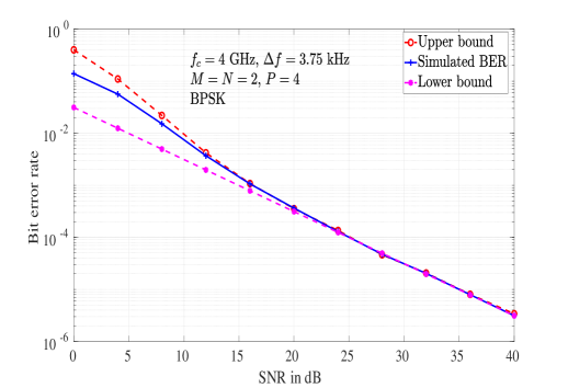
Figure 3: Upper bound, lower bound, and the simulated BER performance of OTFS with $M=N=2$ and $P=4$.

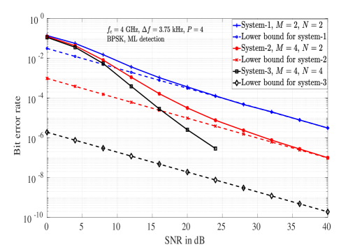
Figure 4: BER performance of OTFS for $i)$ $M=2$, $N=2$, $ii)$ $M=4$, $N=2$, $iii)$ $M=4$, $N=4$.

Figure 4 shows the simulated BER performance of OTFS for different values of $M$ and $N$. We consider the following three systems: $i)$ system-1 with $M=N=2$, $ii)$ system-2 with $M=4$, $N=2$, and $iii)$ system-3 with $M=N=4$. All the three systems use BPSK. The maximum Doppler shift considered is $1/NT$. For system-1 and system-2, which use $N=2$, the maximum Doppler shift is 1.875 kHz, which corresponds to a maximum speed of 506.25 km/h. Likewise, the maximum Doppler shift in the case of system-3 which uses $N=4$ is 938 kHz, corresponding to a maximum speed of 253.125 km/h at 4 GHz carrier frequency. The lower bounds given by (37) for all the three systems are also plotted. We note that the $\frac{\kappa}{2^{MN}}$ values for the considered systems are $\frac{8}{16}$, $\frac{8}{256}$, and $\frac{8}{65536}$, respectively. For illustration purposes, the $\kappa=8$ pairs of matrices $(\mathbf{X}_{i},\mathbf{X}_{j})$ which result in rank one $\mathbf{\Delta}_{ij}$ matrices for the system with $M=N=2$ are given in Table II. Since the $\frac{\kappa}{2^{MN}}$ values are decreasing for increasing $MN$, (37) indicates that the lower bound for system-3 should lie below that of system-2, which, in turn, should lie below that of system-1. This trend is clearly evident from Fig. 4. Further, as noted before, for all the systems, the BER plots show a diversity order greater than one for low to medium SNR values before it meets the diversity one lower bound. An interesting observation, however, is that the system-3 with higher $M$ and $N$ values achieves a higher diversity order compared to those of systems-1 and 2 before meeting the lower bound. This is because the lower bound for system-3 lies much below the lower bounds for systems-1 and 2, and the BER curve of system-3 falls with greater slope to meet its lower bound. This shows that, though the asymptotic diversity order is one, increasing the value of $MN$ (i.e., increasing the frame size) can lead to higher diversity order in the finite SNR regime, resulting in improved performance for increased frame sizes.

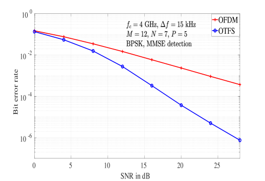
Figure 5: BER performance comparison of OTFS and OFDM systems with MMSE detection for $f_{c}=4$ GHz, $\Delta f=15$ kHz, $M=12$, $N=7$, $P=5$, and BPSK.

III-C Results for practical values of $M$ and $N$ in OTFS

In the previous subsection, we considered small systems with ML detection to illustrate the asymptotic diversity order of OTFS modulation. We now present the performance of OTFS with practical values of $M$ and $N$. In Fig. 5, we present the BER performance of OTFS system with $M=12$ and $N=7$ (smallest resource block used in LTE). A carrier frequency of 4 GHz, a subcarrier spacing of 15 kHz, exponential power delay profile, and Jakes Doppler spectrum [23] are considered. Figure 5 also shows the BER performance of OFDM system for comparison. Both the systems use minimum mean square error (MMSE) detection at the receiver. The maximum Doppler considered is 1.85 kHz, which corresponds to a speed of 500 km/h at 4 GHz carrier frequency. The Doppler shift corresponding the $i$th tap is generated using $\nu_{i}=\nu_{\mbox{\scriptsize{max}}}\cos(\theta_{i})$, where $\nu_{\mbox{\scriptsize{max}}}$ is the maximum Doppler shift and $\theta_{i}$ is uniformly distributed over $[-\pi,\pi]$. From the figure, it can be seen that the performance of OTFS is significantly superior compared to the performance of OFDM. For example, OTFS achieves an SNR gain of about 4 dB and 9 dB compared to OFDM at a BER of $10^{-2}$ and $10^{-3}$, respectively.

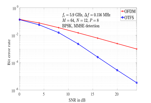
Figure 6: BER performance comparison of OTFS and OFDM systems with MMSE detection for $f_{c}=5.9$ GHz, $\Delta f=0.156$ MHz, $M=64$, $N=12$, $P=8$, and BPSK.

Next, in Fig. 6, we compare the BER performance of OTFS and OFDM considering the system parameters according to the IEEE 802.11p standards, which is a standard for wireless access in vehicular environments (WAVE) [24]. A carrier frequency of 5.9 GHz, a subcarrier frequency of 0.156 MHz, a frame size $(M,N)=(64,12)$, number of paths $P=8$, a maximum speed of 220 km/h, and BPSK are considered. In this WAVE system setting also, we observe that the performance of OTFS is significantly better compared to that of OFDM. For example, OTFS achieves an SNR gain of about 5 dB and 10 dB compared to OFDM at a BER of $10^{-2}$ and $10^{-3}$, respectively. Note that, for the values of $M$, $N$ used in practice (e.g., $M=12$, $N=7$ in LTE and $M=64$, $N=12$ in IEEE 802.11p) and ML detection, the transition of the BER slope to diversity one will take place at very high SNR values. In coded systems, this uncoded BER performance advantage in OTFS can allow the use of high rate codes (e.g., rate 3/4, 7/8) in OTFS systems to achieve a given coded BER performance. A performance comparison between OTFS and OFDM in coded settings is presented in Fig. 3 of [25], where it is shown that OTFS achieves better performance compared to OFDM in coded settings as well.

IV Phase rotation for full diversity in OTFS

In the previous section, we showed that the asymptotic diversity of OTFS is one, and that potential for higher diversity orders is observed in the finite SNR regime for large frame sizes before the diversity one regime takes over. In this section, we propose a ‘phase rotation’ scheme which extracts the full diversity offered by the delay-Doppler channel. From the diversity analysis in Sec. III, it is clear that the asymptotic diversity order of OTFS depends on the minimum rank of the difference matrix $\mathbf{\Delta}_{ij}=(\mathbf{X}_{i}-\mathbf{X}_{j})$, over all pairs of symbol matrices $(\mathbf{X}_{i},\mathbf{X}_{j})$. In order to design a scheme that can extract full diversity, we take a closer look at the symbol matrix $\mathbf{X}$ whose $i$th column is given by (23). The symbol matrix $\mathbf{X}$ is a $P\times MN$ matrix that has only $MN$ unique entries, which are nothing but the $MN$ symbols of the transmit vector $\mathbf{x}$. The rows of the matrix $\mathbf{X}$ are the permutations of the transmit symbol vector $\mathbf{x}$. When $P=MN$, the matrix $\mathbf{X}$ is a block circulant matrix with circulant blocks, as shown in (40). Note that $\mathbf{X}$ has $M$ circulant blocks, each of size $N\times N$, which are cyclically shifted to form a block circulant matrix. In (40), $x_{q}^{(l)}$ denotes the $q$th distinct element of the $l$th block, where $q=0,\cdots,N-1$ and $l=0,\cdots,M-1$. When $P<MN$, the $P$ rows of the matrix $\mathbf{X}$ are a subset of rows from (40), and the selected subset depends on the positions of non-zero entries in the delay-Doppler channel matrix. This structure of $\mathbf{X}$ arises naturally from OTFS pre- and post-processing operations (ISFFT and SFFT) which result in the 2D circular convolution of the transmit vector $\mathbf{x}$ with the channel response in delay-Doppler domain.

$$\mathbf{X}=\left[\begin{array}[]{c|c|c|c}\begin{array}[]{cccc}x_{0}^{(0)}&x_{1}^{(0)}&\cdots&x_{N-1}^{(0)}\\ x_{N-1}^{(0)}&x_{0}^{(0)}&\cdots&x_{N-2}^{(0)}\\ &&\vdots&\\ x_{1}^{(0)}&x_{2}^{(0)}&\cdots&x_{0}^{(0)}\end{array}&\begin{array}[]{cccc}x_{0}^{(1)}&&\cdots&x_{N-1}^{(1)}\\ x_{N-1}^{(1)}&&\cdots&x_{N-2}^{(1)}\\ &&\vdots&\\ x_{1}^{(1)}&&\cdots&x_{0}^{(1)}\end{array}&\cdots&\begin{array}[]{cccc}x_{0}^{(M-1)}&&\cdots&x_{N-1}^{(M-1)}\\ x_{N-1}^{(M-1)}&&\cdots&x_{N-2}^{(M-1)}\\ &&\vdots&\\ x_{1}^{(M-1)}&&\cdots&x_{0}^{(M-1)}\end{array}\\ \hline\cr{\scriptsize\begin{array}[]{cccc}x_{0}^{(M-1)}&x_{1}^{(M-1)}&\cdots&x_{N-1}^{(M-1)}\\ x_{N-1}^{(M-1)}&x_{0}^{(M-1)}&\cdots&x_{N-2}^{(M-1)}\\ &&\vdots&\\ x_{1}^{(M-1)}&x_{2}^{(M-1)}&\cdots&x_{0}^{(M-1)}\end{array}}&\begin{array}[]{cccc}x_{0}^{(0)}&&\cdots&x_{N-1}^{(0)}\\ x_{N-1}^{(0)}&&\cdots&x_{N-2}^{(0)}\\ &&\vdots&\\ x_{1}^{(0)}&&\cdots&x_{0}^{(0)}\end{array}&\cdots&\begin{array}[]{cccc}x_{0}^{(M-2)}&&\cdots&x_{N-1}^{(M-2)}\\ x_{N-1}^{(M-2)}&&\cdots&x_{N-2}^{(M-2)}\\ &&\vdots&\\ x_{1}^{(M-2)}&&\cdots&x_{0}^{(M-2)}\end{array}\\ \hline\cr\vdots&\vdots&\vdots&\vdots\\ \hline\cr\begin{array}[]{cccc}x_{0}^{(1)}&x_{1}^{(1)}&\cdots&x_{N-1}^{(1)}\\ x_{N-1}^{(1)}&x_{0}^{(1)}&\cdots&x_{N-2}^{(1)}\\ &&\vdots&\\ x_{1}^{(1)}&x_{2}^{(1)}&\cdots&x_{0}^{(1)}\end{array}&\begin{array}[]{cccc}x_{0}^{(2)}&&\cdots&x_{N-1}^{(2)}\\ x_{N-1}^{(2)}&&\cdots&x_{N-2}^{(2)}\\ &&\vdots&\\ x_{1}^{(2)}&&\cdots&x_{0}^{(2)}\end{array}&\cdots&\begin{array}[]{cccc}x_{0}^{(0)}&&\cdots&x_{N-1}^{(0)}\\ x_{N-1}^{(0)}&&\cdots&x_{N-2}^{(0)}\\ &&\vdots&\\ x_{1}^{(0)}&&\cdots&x_{0}^{(0)}\end{array}\end{array}\right].$$ (40)

The $MN\times 1$ OTFS transmit vector corresponding to symbol matrix $\mathbf{X}$ in (40) is given by

$$\mathbf{x}=[x_{0}^{(0)},\cdots,x_{N-1}^{(0)},x_{0}^{(1)},\cdots,x_{N-1}^{(1)},\cdots,x_{N-1}^{(M-1)}]^{T}.\vspace{-2mm}$$ (41)

The following theorem shows that multiplying the OTFS transmit vector in (41) by a diagonal phase rotation matrix $\mathbf{\Phi}$ with distinct transcendental numbers results in full diversity.

Theorem 1.

Let

$$\mathbf{\Phi}=\textnormal{diag}\left\{\phi_{0}^{(0)},\cdots,\phi_{N-1}^{(0)},\phi_{0}^{(1)},\cdots,\phi_{N-1}^{(1)},\cdots,\phi_{N-1}^{(M-1)}\right\}$$ (42)

be the phase rotation matrix and

$$\mathbf{x}^{\prime}=\mathbf{\Phi}\mathbf{x}=\begin{bmatrix}\phi_{0}^{(0)}x_{0}^{(0)}\\ \vdots\\ \phi_{N-1}^{(0)}x_{N-1}^{(0)}\\ \phi_{0}^{(1)}x_{0}^{(1)}\\ \vdots\\ \phi_{N-1}^{(1)}x_{N-1}^{(1)}\\ \vdots\\ \phi_{N-1}^{(M-1)}x_{N-1}^{(M-1)}\end{bmatrix}$$ (43)

be the phase rotated OTFS transmit vector. OTFS with the above phase rotation achieves the full diversity of $P$ when $\phi_{q}^{(l)}=e^{ja_{q}^{(l)}}$, $q=0,\cdots,N-1$, $l=0,\cdots,M-1$ are transcendental numbers with $a_{q}^{(l)}$ real, distinct, and algebraic.

Proof.

Let $\mathbf{x}^{\prime}_{i}=\mathbf{\Phi x}_{i}$ and $\mathbf{x}^{\prime}_{j}=\mathbf{\Phi x}_{j}$ be two phase rotated OTFS transmit vectors. Let $\mathbf{X}^{\prime}_{i}$ and $\mathbf{X}^{\prime}_{j}$ denote the corresponding phase rotated symbol matrices.
Case 1: $P=MN$

When $P=MN$, the symbol matrices $\mathbf{X}^{\prime}_{i}$ and $\mathbf{X}^{\prime}_{j}$ are block circulant with circulant blocks, and hence $\mathbf{\Delta}^{\prime}_{ij}=\mathbf{X}^{\prime}_{i}-\mathbf{X}^{\prime}_{j}$ also has the same structure, i.e.,

$$\mathbf{\Delta}^{\prime}_{ij}=\left[\begin{array}[]{c|c|c|c}\mathbf{\Delta^{\prime}}_{ij}^{(0)}&\mathbf{\Delta^{\prime}}_{ij}^{(1)}&\dots&\mathbf{\Delta^{\prime}}_{ij}^{(M-1)}\\ \hline\cr\mathbf{\Delta^{\prime}}_{ij}^{(M-1)}&\mathbf{\Delta^{\prime}}_{ij}^{(0)}&\dots&\mathbf{\Delta^{\prime}}_{ij}^{(M-2)}\\ \hline\cr\vdots&\vdots&\vdots&\vdots\\ \hline\cr\mathbf{\Delta^{\prime}}_{ij}^{(1)}&\mathbf{\Delta^{\prime}}_{ij}^{(2)}&\dots&\mathbf{\Delta^{\prime}}_{ij}^{(0)}\\ \end{array}\right],$$ (44)

where

$$\mathbf{\Delta^{\prime}}_{ij}^{(l)}=\left[\begin{array}[]{cccc}\delta_{0}^{(l)}\phi_{0}^{(l)}&\delta_{1}^{(l)}\phi_{1}^{(l)}&\dots&\delta_{N-1}^{(l)}\phi_{N-1}^{(l)}\\ \delta_{N-1}^{(l)}\phi_{N-1}^{(l)}&\delta_{0}^{(l)}\phi_{0}^{(l)}&\dots&\delta_{N-2}^{(l)}\phi_{N-2}^{(l)}\\ &\vdots&\vdots&\\ \delta_{1}^{(l)}\phi_{1}^{(l)}&\delta_{2}^{(l)}\phi_{2}^{(l)}&\dots&\delta_{0}^{(l)}\phi_{0}^{(l)}\\ \end{array}\right],$$ (45)

where $\delta_{q}^{(l)}=x_{i,q}^{(l)}-x_{j,q}^{(l)}$, with $x_{i,q}^{(l)}$ and $x_{j,q}^{(l)}$ being $q$th distinct elements in the $l$th block of $\mathbf{X}_{i}$ and $\mathbf{X}_{j}$, respectively. Since $\mathbf{\Delta^{\prime}}_{ij}$ is block circulant with circulant blocks, it is diagonalized by $\mathbf{F}_{M}\otimes\mathbf{F}_{N}$, where $\mathbf{F}_{M}$ and $\mathbf{F}_{N}$ denote the $M\times M$ and $N\times N$ DFT matrices and $\otimes$ denotes the Kronecker product. Therefore, $\mathbf{\Delta^{\prime}}_{ij}$ is given by [26]

$$\mathbf{\Delta^{\prime}}_{ij}=(\mathbf{F}_{M}\otimes\mathbf{F}_{N})^{H}\mathbf{D}(\mathbf{F}_{M}\otimes\mathbf{F}_{N}),$$ (46)

where $\mathbf{D}$ is an $MN\times MN$ diagonal matrix whose entries are eigen values of $\mathbf{\Delta^{\prime}}_{ij}$, given by

$$\mathbf{D}=\sum_{l=0}^{M-1}\mathbf{\Omega}_{M}^{l}\otimes\mathbf{\Lambda}^{(l)},$$ (47)

where $\mathbf{\Omega}_{M}=\mbox{diag}\{1,\omega,\omega^{2},\cdots,\omega^{M-1}\}$ with $\omega=e^{j2\pi/M}$, and $\mathbf{\Lambda}^{(l)}$ is a diagonal matrix whose entries are the eigen values of $\mathbf{\Delta^{\prime}}_{ij}^{(l)}$. Let $\lambda_{q}^{(l)}$ denote the $q$th eigen value of $\mathbf{\Delta^{\prime}}_{ij}^{(l)}$ and $\mu_{0},\mu_{1},\cdots,\mu_{MN-1}$ denote the eigen values of $\mathbf{\Delta^{\prime}}_{ij}$. From (47), the $k$th eigen value of $\mathbf{\Delta^{\prime}}_{ij}$, that is, $\mu_{k}$ is given by

$$\mu_{k}=\sum_{l=0}^{M-1}\lambda_{u}^{(l)}\omega^{vl},$$ (48)

where $u=k-\lfloor\frac{k}{N}\rfloor N$, $v=\lfloor\frac{k}{N}\rfloor$, and $\lambda_{u}^{(l)}$ is the $u$th eigen value of $\mathbf{\Delta^{\prime}}_{ij}^{(l)}$, given by

$$\lambda_{u}^{(l)}=\sum_{q=0}^{N-1}\phi_{q}^{(l)}\delta_{q}^{(l)}e^{-j2\pi uq/N}.$$ (49)

Using (49) in (48), we have

$$\mu_{k} = \sum_{l=0}^{M-1}\sum_{q=0}^{N-1}\phi_{q}^{(l)}\delta_{q}^{(l)}e^{-j2\pi uq/N}\omega^{vl}$$ (50)

$$= \sum_{l=0}^{M-1}\bigg{\{}\phi_{0}^{(l)}\delta_{0}^{(l)}+\phi_{1}^{(l)}\delta_{1}^{(l)}e^{-j2\pi u/N}+$$

$$\cdots+\phi_{N-1}^{(l)}\delta_{N-1}^{(l)}e^{-j2\pi u(N-1)/N}\bigg{\}}\omega^{vl},$$

which can be further simplified as

$$\mu_{k} = \phi_{0}^{(0)}\delta_{0}^{(0)}+\phi_{1}^{(0)}\delta_{1}^{(0)}e^{-\frac{j2\pi u}{N}}+$$

$$\cdots+\phi_{N-1}^{(0)}\delta_{N-1}^{(0)}e^{-\frac{j2\pi u(N-1)}{N}}+\ \phi_{0}^{(1)}\delta_{0}^{(1)}\omega^{v}+$$

$$\cdots+\phi_{N-1}^{(1)}\delta_{N-1}^{(1)}e^{-\frac{j2\pi u(N-1)}{N}}\omega^{v}+$$

$$\cdots+\phi_{0}^{(M-1)}\delta_{0}^{(M-1)}\omega^{v(M-1)}+$$ (51)

$$\cdots+\ \phi_{N-1}^{(M-1)}\delta_{N-1}^{(M-1)}e^{-\frac{j2\pi u(N-1)}{N}}\omega^{v(M-1)}.$$

At this stage, we invoke the Lindenmann’s theorem [27], which states that, if $a_{1},a_{2},\cdots,a_{m}$ are distinct algebraic numbers, and if $c_{1},c_{2},\cdots,c_{m}$ are algebraic and not all equal to zero, then

$$c_{1}e^{a_{1}}+c_{2}e^{a_{2}}+\cdots+c_{m}e^{a_{m}}\neq 0.\vspace{-1mm}$$ (52)

It should be noted from (51) that the terms of the form $\delta_{q}^{(l)}e^{-\frac{j2\pi uq}{N}}\omega^{vl}$ are all algebraic [27]. Therefore, comparing (52) and (51), if the terms $\phi_{q}^{(l)}$ are chosen such that $\phi_{q}^{(l)}=e^{ja_{q}^{(l)}}$ are transcendental with $a_{q}^{(l)}$ real, distinct, and algebraic, then $\mu_{k}$ can not be zero. Since $\mu_{k}$s are eigen values of $\mathbf{\Delta^{\prime}}_{ij}$, choosing the diagonal phase rotation matrix with entries $\phi_{q}^{(l)}=e^{ja_{q}^{(l)}}$ being transcendental with $a_{q}^{(l)}$ real, distinct, and algebraic ensures that all the eigen values of $\mathbf{\Delta^{\prime}}_{ij}$ are non-zero, making it full rank (i.e., rank $P$). Since this is true for $\mathbf{\Delta^{\prime}}_{ij}$ for all $(i,j)$, $i\neq j$, the minimum rank of $\mathbf{\Delta^{\prime}}_{ij}$ is equal to $MN$. Hence, from (32), the achieved diversity order of OTFS with the proposed phase rotation is $MN$.
Case 2: $P<MN$

Now, consider the case when $P<MN$. As mentioned previously, when $P<MN$, the rows of the transmit symbol matrix $\mathbf{X}$ is the subset of rows from the corresponding $MN\times MN$ matrix in (40). If $\mathbf{X}^{\prime}_{i}$ and $\mathbf{X}^{\prime}_{j}$ are two phase rotated symbol matrices with $P<MN$, then the rows of $\mathbf{\Delta}^{\prime}_{ij}=\mathbf{X}^{\prime}_{i}-\mathbf{X}^{\prime}_{j}$ form a subset of the rows of the corresponding $MN\times MN$ matrix in (44). Since the matrix in (44) is shown to be full rank in Case 1, $\mathbf{\Delta}^{\prime}_{ij}$ with $P<MN$ should have a rank equal to $P$. Therefore, OTFS with phase rotation using transcendental numbers of the form $\phi_{q}^{(l)}=e^{ja_{q}^{(l)}}$ with $a_{q}^{(l)}$ real, distinct, and algebraic achieves the full diversity of $P$ in the delay-Doppler domain. ∎

IV-A Simulation results

Figure 7 shows the simulated BER performance of OTFS without and with phase rotation for $i)$ system-1 with $M=N=2$, $ii)$ system-2 with $M=4$, $N=2$, and $iii)$ system-3 with $M=N=4$. The carrier frequency and the subcarrier spacing used are 4 GHz and 3.75 kHz, respectively. All the systems use BPSK. Other simulation parameters are as given in Table I. For the simulations, all the three systems use the phase rotation matrix, $\mathbf{\Phi}=\ \textnormal{diag}\{{1,e^{j\frac{1}{MN}}\cdots e^{j\frac{MN-1}{MN}}}\}$. From Fig. 7, we observe that the asymptotic diversity order of all the three systems without phase rotation is one. Further, the OTFS systems with phase rotation exhibit full diversity in the high SNR regime. Although all the systems with phase rotation exhibit a diversity order of $P=4$, we observe a slight difference in the BER performance of the three systems. This is because of the different coding gains achieved by each system. While the proposed phase rotation scheme achieves full delay-Doppler diversity, the coding gain achieved by a system can be improved by optimizing the phases used in the phase rotation matrix [27].

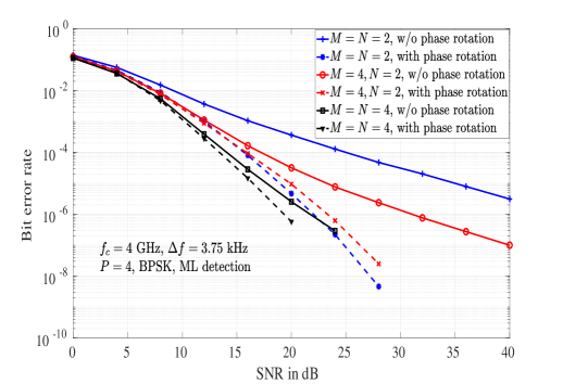
Figure 7: BER performance of OTFS without and with phase rotation for $i)$ $M=N=2$, $ii)$ $M=4$, $N=2$, and $iii)$ $M=N=4$, and BPSK.

In Fig. 8, we present the simulated BER performance of OTFS with and without phase rotation for a system with $M=N=2$ and 8-QAM. The carrier frequency and the subcarrier spacing used are 4 GHz and 3.75 kHz, respectively. Other simulation parameters are as given in Table I. For the simulations, the phase rotation matrix, $\mathbf{\Phi}=\textnormal{diag}\{{1,e^{j\frac{1}{MN}}\cdots e^{j\frac{MN-1}{MN}}}\}$ is used. From Fig. 8, we observe that OTFS without phase rotation achieves a diversity order of one. Whereas, OTFS with phase rotation shows the intended diversity benefit. For example, at a BER of $10^{-5}$, the OTFS system with phase rotation achieves an SNR gain of about 17 dB compared to the system without phase rotation.

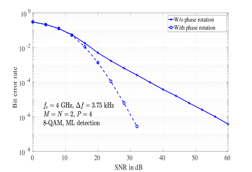
Figure 8: BER performance of OTFS without and with phase rotation, $M=N=2$, and 8-QAM.

V MIMO-OTFS modulation

In this section, we consider OTFS modulation and its diversity order in a MIMO setting.

V-A MIMO-OTFS system model

Consider a MIMO-OTFS system shown in Fig. 9 with $n_{t}$ transmit and $n_{r}$ receive antennas. Each antenna transmits an independent OTFS signal vector. The channel gain between the $k$th transmit antenna and $l$th receive antenna in the delay-Doppler domain corresponding to delay $\tau$ and Doppler $\nu$ is given by

$$h_{lk}(\tau,\nu)=\sum_{i=1}^{P}h_{lk_{i}}\delta(\tau-\tau_{i})\delta(\nu-\nu_{i}),$$ (53)

$k=1,2,\cdots,n_{t}$, $l=1,2,\cdots,n_{r}$, and $P$ is the number of channel taps. Let $\mathbf{H}_{lk}$ denote the $MN\times MN$ equivalent channel matrix between the $k$th transmit antenna and $l$th receive antenna. Let $\mathbf{x}_{k}$ denote the $MN\times 1$ transmit vector from the $k$th transmit antenna and $\mathbf{y}_{l}$ denote the $MN\times 1$ received vector at the $l$th receive antenna. Then, using the linear vector channel model in (21) for SISO-OTFS, the linear system model describing the input and output relation in MIMO-OTFS can be obtained as

$$\mathbf{y}_{1} = \mathbf{H}_{11}\mathbf{x}_{1}+\mathbf{H}_{12}\mathbf{x}_{2}+\cdots+\mathbf{H}_{1{n_{t}}}\mathbf{x}_{n_{t}}+\mathbf{v}_{1},$$

$$\mathbf{y}_{2} = \mathbf{H}_{21}\mathbf{x}_{1}+\mathbf{H}_{22}\mathbf{x}_{2}+\cdots+\mathbf{H}_{2{n_{t}}}\mathbf{x}_{n_{t}}+\mathbf{v}_{2},$$ (54)

$$\vdots$$

$$\mathbf{y}_{n_{r}} = \mathbf{H}_{{n_{r}}1}\mathbf{x}_{1}+\mathbf{H}_{{n_{r}}2}\mathbf{x}_{2}+\cdots+\mathbf{H}_{{n_{r}}{n_{t}}}\mathbf{x}_{n_{t}}+\mathbf{v}_{n_{r}}.\hskip 11.38109pt$$

Defining

$$\ \mathbf{H}_{{\tiny\mbox{MIMO}}} =\begin{bmatrix}\mathbf{H}_{11}&\mathbf{H}_{12}&\dots&\mathbf{H}_{1{n_{t}}}\\ \mathbf{H}_{21}&\mathbf{H}_{22}&\dots&\mathbf{H}_{2{n_{t}}}\\ \vdots&\vdots&\ddots&\vdots\\ \mathbf{H}_{{n_{r}}1}&\mathbf{H}_{{n_{r}}2}&\dots&\mathbf{H}_{{n_{r}}{n_{t}}}\end{bmatrix},$$

$\mathbf{x}_{{\tiny\mbox{MIMO}}}={[{\mathbf{x}_{1}}^{T},{\mathbf{x}_{2}}^{T},\cdots,{\mathbf{x}_{n_{t}}}^{T}]}^{T}$, $\mathbf{y}_{{\tiny\mbox{MIMO}}}={[{\mathbf{y}_{1}}^{T},{\mathbf{y}_{2}}^{T},\cdots,{\mathbf{y}_{n_{r}}}^{T}]}^{T}$, $\mathbf{v}_{{\tiny\mbox{MIMO}}}={[{\mathbf{v}_{1}}^{T},{\mathbf{v}_{2}}^{T},\cdots,{\mathbf{v}_{n_{r}}}^{T}]}^{T}$, (54) can be written as

$$\mathbf{y}_{{\tiny\mbox{MIMO}}}=\mathbf{H}_{{\tiny\mbox{MIMO}}}\mathbf{x}_{{\tiny\mbox{MIMO}}}+\mathbf{v}_{\tiny\mbox{MIMO}},$$ (55)

where $\mathbf{x}_{{\tiny\mbox{MIMO}}}\in\mathbb{C}^{{n_{t}}MN\times 1},\mathbf{y}_{{\tiny\mbox{MIMO}}},\mathbf{v}_{\tiny\mbox{MIMO}}\in\mathbb{C}^{{n_{r}}MN\times 1}$, and $\mathbf{H}_{{\tiny\mbox{MIMO}}}\in\mathbb{C}^{{n_{r}}MN\times{n_{t}}MN}$.

Figure 9: MIMO-OTFS modulation scheme.

V-B Diversity of MIMO-OTFS

In this subsection, we derive the asymptotic diversity order of MIMO-OTFS. For this, first note that, in the effective channel matrix $\mathbf{H}_{\tiny\mbox{MIMO}}$, each $\mathbf{H}_{lk}$ has only $P$ unique entries, and hence $\mathbf{H}_{\tiny\mbox{MIMO}}$ has $Pn_{t}n_{r}$ unique entries. Further, each row of $\mathbf{H}_{{\tiny\mbox{MIMO}}}$ has only $n_{t}P$ non-zero elements and each column has only $n_{r}P$ non-zero elements. Following (22), the MIMO-OTFS system model in (55) can be written as

$$\begin{bmatrix}\mathbf{y}_{1}^{T}\\ \mathbf{y}_{2}^{T}\\ \vdots\\ \mathbf{y}_{n_{r}}^{T}\end{bmatrix}=\begin{bmatrix}\mathbf{h}^{\prime}_{11}&\mathbf{h}^{\prime}_{12}\cdots\mathbf{h}^{\prime}_{1n_{t}}\\ \mathbf{h}^{\prime}_{21}&\mathbf{h}^{\prime}_{22}\cdots\mathbf{h}^{\prime}_{2n_{t}}\\ \vdots\\ \mathbf{h}^{\prime}_{n_{r}1}&\mathbf{h}^{\prime}_{n_{r}2}\cdots\mathbf{h}^{\prime}_{n_{r}n_{t}}\\ \end{bmatrix}\begin{bmatrix}\mathbf{X}_{1}\\ \mathbf{X}_{2}\\ \vdots\\ \mathbf{X}_{n_{t}}\end{bmatrix}+\begin{bmatrix}\mathbf{v}_{1}^{T}\\ \mathbf{v}_{2}^{T}\\ \vdots\\ \mathbf{v}_{n_{r}}^{T}\end{bmatrix},$$ (56)

or equivalently

$${\tilde{\bf y}}={\tilde{\bf H}}{\tilde{\bf X}}+\tilde{\mathbf{V}},$$ (57)

where ${\tilde{\bf y}}$ is an $n_{r}\times MN$ received signal matrix whose $l$th row is the received vector received in the $l$th receive antenna, ${\tilde{\bf X}}$ is an $n_{t}P\times MN$ matrix obtained by stacking $n_{t}$ number of $P\times MN$ sized symbol matrices of the form (23), ${\tilde{\bf H}}\in\mathbb{C}^{n_{r}\times n_{t}P}$ is the channel matrix with $\mathbf{h}^{\prime}_{lk}\in\mathbb{C}^{1\times P}$ consisting of $P$ unique non-zero entries of $\mathbf{H}_{lk}$, and ${\tilde{\bf V}}\in\mathbb{C}^{n_{r}\times MN}$ is the noise matrix.

Let $\tilde{\mathbf{X}}_{i}$ and $\tilde{\mathbf{X}}_{j}$ be two symbol matrices. Assuming perfect channel state information and ML detection at the receiver, the probability of decoding the transmitted symbol matrix $\tilde{\mathbf{X}}_{i}$ in favor of $\tilde{\mathbf{X}}_{j}$ is given by

$$P(\tilde{\mathbf{X}}_{i}\rightarrow\tilde{\mathbf{X}}_{j}|\tilde{\mathbf{H}})=Q\left(\sqrt{\frac{\|\tilde{\mathbf{H}}(\tilde{\mathbf{X}}_{i}-\tilde{\mathbf{X}}_{j})\|^{2}}{2N_{0}}}\right),$$ (58)

and the average PEP is given by

$$P(\tilde{\mathbf{X}}_{i}\rightarrow\tilde{\mathbf{X}}_{j})=\mathbb{E}\left[Q\left(\sqrt{\frac{\|\tilde{\mathbf{H}}(\tilde{\mathbf{X}}_{i}-\tilde{\mathbf{X}}_{j})\|^{2}}{2N_{0}}}\right)\right].$$ (59)

Using Chernoff bound and the fact that each antenna transmits independent OTFS symbols, an upper bound on the PEP in (59) can be obtained as [22]

$$P(\tilde{\mathbf{X}}_{i}\rightarrow\tilde{\mathbf{X}}_{j})\leq\left(\prod\limits_{l=1}^{r}\frac{1}{1+\frac{\gamma\lambda_{k,l}^{2}}{4P}}\right)^{n_{r}},$$ (60)

where $\gamma=\frac{1}{N_{0}}$ is the SNR per receive antenna, $\lambda_{k,l}$ is the $l$th singular value of the difference matrix $\mathbf{\Delta}_{k,ij}=(\mathbf{X}_{k,i}-\mathbf{X}_{k,j})$ with $\mathbf{X}_{k,i}$ and $\mathbf{X}_{k,j}$ denoting OTFS symbol matrices transmitted from $k$th antenna (for some $k\in{1,2,\cdots,n_{t}}$) in $\tilde{\mathbf{X}}_{i}$ and $\tilde{\mathbf{X}}_{j}$, respectively, and $r$ is the rank of $\mathbf{\Delta}_{k,ij}$. At high SNR values, (60) simplifies to

$$P(\tilde{\mathbf{X}}_{i}\rightarrow\tilde{\mathbf{X}}_{j})\leq\frac{1}{\gamma^{n_{r}r}}\left(\prod_{l=1}^{r}\frac{\lambda_{k,l}^{2}}{4P}\right)^{-n_{r}}.$$ (61)

The PEP term with the minimum value of $r$ dominates the overall BER. Therefore, the diversity order achieved by MIMO-OTFS, denoted by $\rho_{\tiny\mbox{mimo-otfs}}$ is given by

$$\rho_{\tiny\mbox{mimo-otfs}}=n_{r}\cdot\min_{i,j\ i\neq j}\ \mbox{rank}(\mathbf{\Delta}_{k,ij}).$$ (62)

Now, similar to the case of SISO-OTFS, if $\mathbf{X}_{k,i}=a.\mathbf{1}_{P\times MN}$ and $\mathbf{X}_{k,j}=a^{\prime}.\mathbf{1}_{P\times MN}$, then the difference matrix $\mathbf{\Delta}_{k,ij}=(a-a^{\prime}).\mathbf{1}_{P\times MN}$ has rank one. Hence, the asymptotic diversity order of MIMO-OTFS is $n_{r}$.                                        $\square$

V-C Phase rotation for full diversity in MIMO-OTFS

In this subsection, we consider phase rotation to extract the full diversity in MIMO-OTFS. The transmit vector in MIMO-OTFS is a concatenation of $n_{t}$ independent OTFS transmit vectors of size $MN\times 1$ as described by (55). The $MN\times 1$ OTFS transmit vector from each antenna is multiplied by the phase rotation matrix $\mathbf{\Phi}$ given in (42). The phase rotated MIMO-OTFS transmit vector is then given by

$$\mathbf{x}^{\prime}_{\tiny\mbox{{MIMO}}}=(\mathbf{I}_{n_{t}}\otimes\mathbf{\Phi})\mathbf{x}_{\tiny\mbox{{MIMO}}}.$$ (63)

Let $\tilde{\mathbf{X}}^{\prime}$ be the phase rotated MIMO-OTFS symbol matrix corresponding to $\mathbf{x}^{\prime}$. From (56), $\tilde{\mathbf{X}}^{\prime}$ is of the form

$$\tilde{\mathbf{X}}^{\prime}=\begin{bmatrix}\mathbf{X}^{\prime}_{1}\\ \mathbf{X}^{\prime}_{2}\\ \vdots\\ \mathbf{X}^{\prime}_{n_{t}}\end{bmatrix},$$ (64)

where $\mathbf{X}^{\prime}_{k}$ is the phase rotated OTFS symbol matrix corresponding to the $k$th transmit antenna. If $\tilde{\mathbf{X}}^{\prime}_{i}$ and $\tilde{\mathbf{X}}^{\prime}_{j}$ are two phase rotated MIMO-OTFS symbol matrices corresponding to the transmit vectors $\mathbf{x}^{\prime}_{i,\tiny{\mbox{MIMO}}}$ and $\mathbf{x}^{\prime}_{j,\tiny{\mbox{MIMO}}}$, then their difference matrix $\tilde{\mathbf{\Delta}}^{\prime}_{ij}$ is of the form

$$\tilde{\mathbf{\Delta}}^{\prime}_{ij}=\begin{bmatrix}\mathbf{\Delta}^{\prime}_{1,ij}\\ \mathbf{\Delta}^{\prime}_{2,ij}\\ \vdots\\ \mathbf{\Delta}^{\prime}_{n_{t},ij}\end{bmatrix},$$ (65)

where $\mathbf{\Delta}^{\prime}_{k,ij}=\mathbf{X}^{\prime}_{k,i}-\mathbf{X}^{\prime}_{k,j}$, with $\mathbf{X}^{\prime}_{k,i}$ and $\mathbf{X}^{\prime}_{k,j}$ being the phase rotated OTFS symbol matrices corresponding to the $k$th antenna in $\tilde{\mathbf{X}}^{\prime}_{i}$ and $\tilde{\mathbf{X}}^{\prime}_{j}$, respectively. From Sec. IV, it is known that $\mathbf{\Delta}^{\prime}_{k,ij}$ has rank equal to $P$ for all $k={1,2,\cdots,n_{t}}$. Using this fact in (62), the diversity order achieved by phase rotated MIMO-OTFS system is equal to $Pn_{r}$.                                                                   $\square$

V-D Simulation results

Figure 10 shows the BER performance of $1\times 1$ SISO-OTFS and $2\times 2$ MIMO-OTFS systems. Both the systems use $M=N=2$ and BPSK. The number of channel taps considered is $P=4$. The carrier frequency and the subcarrier spacing used are 4 GHz and 3.75 kHz, respectively. The considered simulation parameters are summarized in Table I. From the figure, it is observed that the simulated BER for $1\times 1$ SISO-OTFS and $2\times 2$ MIMO-OTFS show diversity orders of one and two, respectively, verifying the analytical diversity order derived in the previous subsection.

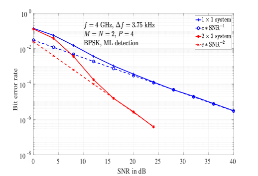
Figure 10: BER performance of $1\times 1$ SISO-OTFS and $2\times 2$ MIMO-OTFS systems.

Next, we consider the effect of increasing the frame size (i.e., $MN$) on the BER performance. Figure 11 shows the BER performance of $1\times 2$ system with $i)$ $M=N=2$ and $ii)$ $M=4$, $N=2$. Both the systems use BPSK. The number of channel taps considered is $P=4$. Other simulation parameters are as given in Table I. From the figure, we observe that the BER performance of the system with $M=4$ and $N=2$ is better than the system with $M=N=2$. This is similar to the SISO-OTFS result shown in Sec. III-B. Specifically, increasing the frame size ($MN$) results in higher diversity order in the finite SNR regime, before the asymptotic diversity order of $\rho_{\tiny\mbox{mimo-otfs}}=2$ takes over. It can be observed that, MIMO-OTFS can achieve diversity orders closer to $Pn_{r}$ in the finite SNR regime, as the size of the OTFS frame $MN$ is increased. Figure 12 shows the BER performance of a $2\times 2$ MIMO-OTFS systems with and without phase rotation with $M=N=2$ and BPSK. From the figure, it can be seen that the MIMO-OTFS system with phase rotation achieves the intended diversity benefit compared to the diversity in MIMO-OTFS without phase rotation.

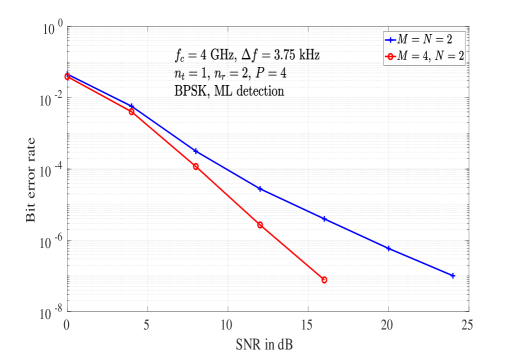
Figure 11: BER performance of $1\times 2$ OTFS system with $i)$ $M=N=2$ and $ii)$ $M=4$, $N=2$.

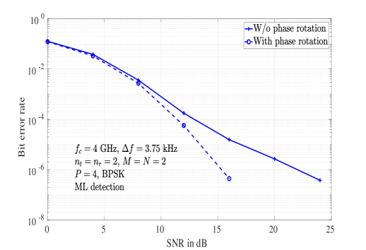
Figure 12: BER performance of $2\times 2$ MIMO-OTFS system without and with phase rotation, $M=N=2$.

VI Conclusions

We investigated the diversity of OTFS modulation and showed that the asymptotic diversity order of OTFS in a SISO setting with ML detection is one. Though the asymptotic diversity order is one, it was found that higher diversity performance can be achieved in the finite SNR regime before the diversity one regime takes over, and that the diversity one regime starts at lower BER values for increased frame sizes. These observations were illustrated through a BER lower bound derived based on diversity one PEPs and simulations. Next, a phase rotation scheme using transcendental numbers was proposed to extract the full diversity offered by the delay-Doppler channel. It was proved that the proposed phase rotation achieves full diversity. Finally, we extended the diversity analysis and results for MIMO-OTFS without and with phase rotation. Timing/frequency offset and synchronization effects and link adaptation in OTFS can be considered for future work. More robust systems targeting ultra-reliable and low-latency communication can be considered with proper configuration for $M$, $N$, coding, and the consideration of the natural presence of residual synchronization effects in combination with the proposed rotation scheme.

Appendix A Diversity Analysis for Non-zero Fractional Delays and Dopplers

Recall the channel representation in the delay-Doppler domain denoted by $h(\tau,\nu)$ in (18). Consider the case of non-zero fractional delays and Dopplers, i.e., consider

$$\tau_{i}=\frac{\alpha_{i}+a_{i}}{M\Delta f},\ \ \mbox{and}\ \ \nu_{i}=\frac{\beta_{i}+b_{i}}{NT},$$ (66)

where $\alpha_{i}=[\tau_{i}M\Delta f]^{\odot}$, $\beta_{i}=[\nu_{i}NT]^{\odot}$, and $[.]^{\odot}$ denotes the nearest integer operator (i.e., rounding operator). Note that $\alpha_{i}$ and $\beta_{i}$ are integers corresponding to the indices of the delay $\tau_{i}$ and Doppler frequency tap $\nu_{i}$, respectively, and $a_{i}$, $b_{i}$ are the fractional delay and Doppler such that $-\frac{1}{2}<a_{i},b_{i},\leq\frac{1}{2}$. With this, we now proceed to derive the input-output relation for OTFS modulation taking into account the fractional part of the delay and Doppler shifts. Substituting (18) and (17) into (16), and assuming rectangular window functions, we get

$$h_{w}(\tau,\nu) = \sum_{i=1}^{P}h_{i}e^{-j2\pi\tau_{i}\nu_{i}}w(\nu-\nu_{i},\tau-\tau_{i})$$ (67)

$$= \sum_{i=1}^{P}h_{i}e^{-j2\pi\tau_{i}\nu_{i}}\mathcal{G}(\nu,\nu_{i})\mathcal{F}(\tau,\tau_{i}),$$

where

$$\mathcal{G}(\nu,\nu_{i}) \triangleq \sum_{n^{\prime}=0}^{N-1}e^{-j2\pi(\nu-\nu_{i})n^{\prime}T},$$

$$\mathcal{F}(\tau,\tau_{i}) \triangleq \sum_{m^{\prime}=0}^{M-1}e^{j2\pi(\tau-\tau_{i})m^{\prime}\Delta f}.$$ (68)

In order to use $h_{w}(\tau,\nu)$ of (67) in the OTFS input-output relation in (14), we need to evaluate $h_{w}(\tau,\nu)$ at $\nu=\frac{k-k^{\prime}}{NT},\tau=\frac{l-l^{\prime}}{M\Delta f}$. Evaluating $\mathcal{G}(\nu,\nu_{i})$ at $\nu=\frac{k-k^{\prime}}{NT}$, we get

$$\mathcal{G}\left(\frac{k-k^{\prime}}{NT},\nu_{i}\right) = \sum_{n^{\prime}=0}^{N-1}e^{-j\frac{2\pi}{N}(k-k^{\prime}-\beta_{i}-b_{i})n^{\prime}}$$ (69)

$$= \frac{e^{-j2\pi(k-k^{\prime}-\beta_{i}-b_{i})}-1}{e^{-j\frac{2\pi}{N}(k-k^{\prime}-\beta_{i}-b_{i})}-1}.$$

Note that due to the fractional Doppler $b_{i}$, for a given $k$, $\mathcal{G}\left(\frac{k-k^{\prime}}{NT},\nu_{i}\right)\neq 0$, for all $k^{\prime}$. It has been shown in [10] that the magnitude of $\mathcal{G}\left(\frac{k-k^{\prime}}{NT},\nu_{i}\right)$ has a peak at $k^{\prime}=k-\beta_{i}$ and decreases as $k^{\prime}$ moves away from $k-\beta_{i}$. Similarly, evaluating $\mathcal{F}(\tau,\tau_{i})$ at $\tau=\frac{l-l^{\prime}}{M\Delta f}$, we get

$$\mathcal{F}\left(\frac{l-l^{\prime}}{M\Delta f},\tau_{i}\right) = \sum_{m^{\prime}=0}^{M-1}e^{j\frac{2\pi}{M}(l-l^{\prime}-\alpha_{i}-a_{i})m^{\prime}}$$ (70)

$$= \frac{e^{j2\pi(l-l^{\prime}-\alpha_{i}-a_{i})}-1}{e^{j\frac{2\pi}{M}(l-l^{\prime}-\alpha_{i}-a_{i})}-1}.$$

Note that due to the fractional delay $a_{i}$, for a given $l$, $\mathcal{F}\left(\frac{l-l^{\prime}}{M\Delta f},\tau_{i}\right)\neq 0$, for all $l^{\prime}$. Using the same argument used for $\mathcal{G}\left(\frac{k-k^{\prime}}{NT},\nu_{i}\right)$, it follows that the magnitude of $\mathcal{F}\left(\frac{l-l^{\prime}}{M\Delta f},\tau_{i}\right)$ has a peak at $l^{\prime}=l-\alpha_{i}$ and decreases as $l^{\prime}$ moves away from $l-\alpha_{i}$. Now, using (69), (70), and (67) in (14), we get

$$y[k,l]= \sum_{i=1}^{P}\sum_{q=0}^{M-1}\sum_{q^{\prime}=0}^{N-1}\left(\frac{e^{j2\pi(-q-a_{i})}-1}{Me^{j\frac{2\pi}{M}(-q-a_{i})}-M}\right)$$

$$\left(\frac{e^{-j2\pi(-q^{\prime}-b_{i})}-1}{Ne^{-j\frac{2\pi}{N}(-q^{\prime}-b_{i})}-N}\right)h_{i}e^{-j2\pi\tau_{i}\nu_{i}}$$

$$x[(k-\beta_{i}+q^{\prime})_{N},(l-\alpha_{i}+q)_{M}].$$ (71)

The input-output equation in (71) can be written in vectorized form as

$$\mathbf{y}=\mathbf{Hx}+\mathbf{v},$$ (72)

where $\mathbf{x}$, $\mathbf{y}$, $\mathbf{v}\in\mathbb{C}^{MN\times 1}$, $\mathbf{H}\in\mathbb{C}^{MN\times MN}$, and the elements of $\mathbf{x}$, $\mathbf{y}$, and $\mathbf{H}$ are determined from (71).

A-A Diversity analysis

The vectorized input-output relation in (72) can be rewritten in an alternate form as

$$\mathbf{y}^{T}=\mathbf{h}^{\prime}\mathbf{X}+\mathbf{v}^{T},$$ (73)

where $\mathbf{y}^{T}$ is $1\times MN$ received vector, $\mathbf{h}^{\prime}$ is a $1\times P$ vector whose $i$th entry is given by $h_{i}e^{-j2\pi\tau_{i}\nu_{i}}$, and $\mathbf{X}$ is a $P\times MN$ matrix whose $i$th column ($i=k+Nl$, $i=0,1,\cdots,MN-1$), denoted by $\mathbf{X}[i]$, is given by (74).

$$\hskip 2.84526pt\mathbf{X}[i]=\begin{bmatrix}\displaystyle\sum_{q=0}^{M-1}\sum_{q^{\prime}=0}^{N-1}\left(\frac{e^{j2\pi(-q-a_{1})}-1}{Me^{j\frac{2\pi}{M}(-q-a_{1})}-M}\right)\left(\frac{e^{-j2\pi(-q^{\prime}-b_{1})}-1}{Ne^{-j\frac{2\pi}{N}(-q^{\prime}-b_{1})}-N}\right)x[(k-\beta_{1}+q^{\prime})_{N},(l-\alpha_{1}+q)_{M}]\\ \displaystyle\sum_{q=0}^{M-1}\sum_{q^{\prime}=0}^{N-1}\left(\frac{e^{j2\pi(-q-a_{2})}-1}{Me^{j\frac{2\pi}{M}(-q-a_{2})}-M}\right)\left(\frac{e^{-j2\pi(-q^{\prime}-b_{2})}-1}{Ne^{-j\frac{2\pi}{N}(-q^{\prime}-b_{2})}-N}\right)x[(k-\beta_{2}+q^{\prime})_{N},(l-\alpha_{2}+q)_{M}]\\ \vdots\\ \displaystyle\sum_{q=0}^{M-1}\sum_{q^{\prime}=0}^{N-1}\left(\frac{e^{j2\pi(-q-a_{P})}-1}{Me^{j\frac{2\pi}{M}(-q-a_{P})}-M}\right)\left(\frac{e^{-j2\pi(-q^{\prime}-b_{P})}-1}{Ne^{-j\frac{2\pi}{N}(-q^{\prime}-b_{P})}-N}\right)x[(k-\beta_{P}+q^{\prime})_{N},(l-\alpha_{P}+q)_{M}]\end{bmatrix}.$$ (74)

The representation of $\mathbf{X}$ in the form given in (73) allows us to view $\mathbf{X}$ as a $P\times MN$ symbol matrix. For convenience, we normalize the elements of $\mathbf{X}$ so that the average energy per symbol time is one. The SNR, denoted by $\gamma$, is therefore given by $\gamma=1/N_{0}$. Assuming perfect channel state information and ML detection at the receiver, the PEP between $\mathbf{X}_{i}$ and $\mathbf{X}_{j}$ is given by

$$P(\mathbf{X}_{i}\rightarrow\mathbf{X}_{j}|\mathbf{h^{\prime}},\mathbf{X}_{i})=Q\left(\sqrt{\frac{\|\mathbf{h^{\prime}}(\mathbf{X}_{i}-\mathbf{X}_{j})\|^{2}}{2N_{0}}}\right).$$ (75)

The PEP averaged over the channel statistics is given by

$$\small P(\mathbf{X}_{i}\rightarrow\mathbf{X}_{j})=\mathbb{E}\left[Q\left(\sqrt{\frac{\gamma\ \|\mathbf{h^{\prime}}(\mathbf{X}_{i}-\mathbf{X}_{j})\|^{2}}{2}}\right)\right].$$ (76)

As in Sec. III, (76) can be obtained as

$$P(\mathbf{X}_{i}\rightarrow\mathbf{X}_{j})=\mathbb{E}\left[Q\left(\sqrt{\frac{\gamma\ \sum_{l=1}^{r}\lambda_{l}^{2}|\tilde{h}_{l}|^{2}}{2}}\right)\right],$$ (77)

where $r$ denotes the rank of the difference matrix $\mathbf{\Delta}_{ij}=(\mathbf{X}_{i}-\mathbf{X}_{j})$, $\tilde{h}_{l}$ is the $l$th element of the vector $\tilde{\bf h}^{H}=\mathbf{U}^{H}\mathbf{h^{\prime}}^{H}$, where the matrix $(\mathbf{X}_{i}-\mathbf{X}_{j})(\mathbf{X}_{i}-\mathbf{X}_{j})^{H}$ is Hermitian matrix that is diagonalizable by unitary transformation and hence can be written as $(\mathbf{X}_{i}-\mathbf{X}_{j})(\mathbf{X}_{i}-\mathbf{X}_{j})^{H}=\mathbf{U\Lambda U}^{H}$, where $\mathbf{U}$ is unitary and $\mathbf{\Lambda}=\mbox{diag}\{\lambda_{1}^{2},\cdots\lambda_{P}^{2}\}$, $\lambda_{i}$ being $i$th singular value of the difference matrix $\mathbf{\Delta}_{ij}$, The average PEP in (77) can be simplified to get the following upper bound on PEP [22]

$$P(\mathbf{X}_{i}\rightarrow\mathbf{X}_{j})\leq\prod\limits_{l=1}^{r}\frac{1}{1+\ \dfrac{\gamma\lambda_{l}^{2}}{4P}},$$ (78)

which, at high SNRs, can be further simplified as

$$P(\mathbf{X}_{i}\rightarrow\mathbf{X}_{j})\leq\frac{1}{\gamma^{r}\prod\limits_{l=1}^{r}\dfrac{\lambda_{l}^{2}}{4P}}.$$ (79)

From (79), it can be seen that the exponent of the SNR term $\gamma$ is $r$, which is equal to the rank of the difference matrix $\mathbf{\Delta}_{ij}$. For all $i,j$, $i\neq j$, the PEP with the minimum value of $r$ dominates the overall BER. Therefore, the achieved diversity order, denoted by $\rho_{\tiny\mbox{siso-otfs}}$, is given by

$$\rho_{\tiny\mbox{siso-otfs}}=\min_{i,j\ i\neq j}\ \mbox{rank}(\mathbf{\Delta}_{ij}).$$ (80)

Now, consider a case when $x_{i}[k,l]=a$ and $x_{j}[k,l]=a^{\prime}$, $\forall k=0,\cdots,N-1$ and $l=0,\cdots,M-1$. Then, $\mathbf{\Delta}_{ij}=(\mathbf{X}_{i}-\mathbf{X}_{j})$ will be of the form $(a-a^{\prime}).\mathbf{Z}_{P\times MN}$, where each column of $\mathbf{Z}$ is identical and of the form given by

$$(a-a^{\prime})\begin{bmatrix}\displaystyle\sum_{q=0}^{M-1}\sum_{q^{\prime}=0}^{N-1}\left(\tfrac{e^{j2\pi(-q-a_{1})}-1}{Me^{j\frac{2\pi}{M}(-q-a_{1})}-M}\right)\left(\tfrac{e^{-j2\pi(-q^{\prime}-b_{1})}-1}{Ne^{-j\tfrac{2\pi}{N}(-q^{\prime}-b_{1})}-N}\right)\\ \displaystyle\sum_{q=0}^{M-1}\sum_{q^{\prime}=0}^{N-1}\left(\tfrac{e^{j2\pi(-q-a_{2})}-1}{Me^{j\frac{2\pi}{M}(-q-a_{2})}-M}\right)\left(\tfrac{e^{-j2\pi(-q^{\prime}-b_{2})}-1}{Ne^{-j\frac{2\pi}{N}(-q^{\prime}-b_{2})}-N}\right)\\ \vdots\\ \displaystyle\sum_{q=0}^{M-1}\sum_{q^{\prime}=0}^{N-1}\left(\tfrac{e^{j2\pi(-q-a_{P})}-1}{Me^{j\frac{2\pi}{M}(-q-a_{P})}-M}\right)\left(\tfrac{e^{-j2\pi(-q^{\prime}-b_{P})}-1}{Ne^{-j\tfrac{2\pi}{N}(-q^{\prime}-b_{P})}-N}\right)\end{bmatrix}.$$ (81)

Since all columns of $\mathbf{Z}$ are identical (independent of $k$ and $l$) with the form (81), rank of $\mathbf{Z}$ is clearly one, which is the minimum rank of $\mathbf{\Delta}_{ij}$, $\forall i,j$, $i\neq j$. Hence, the asymptotic diversity order of OTFS with ML detection in the case of fractional delay and Dopplers is also one.                        $\square$

Simulation results: Figure 13 shows the BER performance with non-zero fractional delays and Dopplers. The figure shows the performance of two systems, $i)$ system-1 with $M=N=2$ and $ii)$ system-2 with $M=4$ and $N=2$. The carrier frequency and the subcarrier spacing used are 4 GHz and 3.75 kHz, respectively. Both the systems use BPSK and ML detection. A channel with $P=4$ paths with a maximum Doppler of 1.875 kHz (which corresponds to a speed of 506.25 km/h at 4 GHz carrier frequency), exponential power delay profile, and Jakes Doppler spectrum [23] is considered. The input-output relation in (71) which considers the fractional part of the delay and Doppler values is used for the simulations. From Fig. 13, it is evident that the asymptotic diversity order of OTFS modulation is one in the case of non-zero fractional delays and Dopplers. Also, the asymptotic diversity order of one is achieved at lower BER values for increased values of $M$ and $N$. This behavior is the same as that observed in Sec. III, where analysis and simulations were carried out without considering fractional delay and Doppler values.

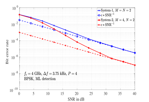
Figure 13: BER performance of OTFS for $i)$ $M=2$, $N=2$ and $ii)$ $M=4$, $N=2$, considering non-zero fractional delay and Doppler values.

References

- [1] W. C. Jakes, Microwave Mobile Communications, New York: IEEE Press, reprinted, 1994.
- [2] T. Wang, J. G. Proakis, E. Masry, and J. R. Zeidler, “Performance degradation of OFDM systems due to Doppler spreading,” IEEE Trans. Wireless Commun., vol. 5, no. 6, pp. 1422-1432, Jun. 2006.
- [3] R. Hadani, S. Rakib, M. Tsatsanis, A. Monk, A. J. Goldsmith, A. F. Molisch, and R. Calderbank, “Orthogonal time frequency space modulation,” in Proc. IEEE WCNC’2017, pp. 1-7, Mar. 2017.
- [4] R. Hadani, S. Rakib, S. Kons, M. Tsatsanis, A. Monk, C. Ibars, J. Delfeld, Y. Hebron, A. J. Goldsmith, A. F. Molisch, and R. Calderbank, “Orthogonal time frequency space modulation,” arXiv:1808.00519v1 [cs.IT] 1 Aug 2018.
- [5] R. Hadani and A. Monk, “OTFS: A new generation of modulation addressing the challenges of 5G,” arXiv:1802.02623 [cs.IT] 7 Feb 2018.
- [6] A. Monk, R. Hadani, M. Tsatsanis, and S. Rakib, “OTFS - orthogonal time frequency space: a novel modulation technique meeting 5G high mobility and massive MIMO challenges,” arXiv:1608.02993 [cs.IT] 9 Aug 2016.
- [7] R. Hadani, S. Rakib, A. F. Molisch, C. Ibars, A. Monk, M. Tsatsanis, J. Delfeld, A. Goldsmith, and R. Calderbank, “Orthogonal time frequency space (OTFS) modulation for millimeter-wave communications systems,” in Proc. IEEE MTT-S Intl. Microwave Symp., pp. 681-683, Jun. 2017.
- [8] L. Li, H. Wei, Y. Huang, Y. Yao, W. Ling, G. Chen, P. Li, and Y. Cai, “A simple two-stage equalizer with simplified orthogonal time frequency space modulation over rapidly time-varying channels,” arXiv:1709.02505v1 [cs.IT] 8 Sep 2017.
- [9] A. Farhang, A. R. Reyhani, L. E. Doyle, and B. Farhang-Boroujeny, “Low complexity modem structure for OFDM-based orthogonal time frequency space modulation,” IEEE Wireless Commun. Lett., vol. 7, no. 3, pp. 344-347, Jun. 2018.
- [10] P. Raviteja, K. T. Phan, Y. Hong, and E. Viterbo, “Interference cancellation and iterative detection for orthogonal time frequency space modulation,” IEEE Trans. Wireless Commun., vol. 17, no. 10, pp. 6501-6515, Aug. 2018.
- [11] K. R. Murali and A. Chockalingam, “On OTFS modulation for high-Doppler fading channels,” in Proc. ITA’2018, Feb. 2018.
- [12] M. K. Ramachandran and A. Chockalingam, “MIMO-OTFS in high-Doppler fading channels: signal detection and channel estimation,” in Proc. IEEE GLOBECOM’2018, Dec. 2018. Online: arXiv:1805.02209v1 [cs.IT] 6 May 2018.
- [13] R. Nissel, S. Schwarz, and M. Rupp, “Filter bank multicarrier modulation schemes for future mobile communications,” IEEE J. Sel. Areas Commun., vol. 35, no. 8, pp. 1768-1782, Aug. 2017.
- [14] N. Michailow, M. Matthe, I. S. Gaspar, A. N. Caldevilla, L. L. Mendes, A. Festag, and G. Fettweis, “Generalized frequency division multiplexing for 5th generation cellular networks,” IEEE Trans. Commun., vol. 62, no. 9, pp. 3045-3061, Sep. 2014.
- [15] A. Nimr, M. Chafii, M. Matthe, and G. Fettweis, “Extended GFDM framework: OTFS and GFDM comparison,” online: arXiv:1808.01161v1 [eess.SP] 3 Aug 2018.
- [16] T. Strohmer and S. Beaver, “Optimal OFDM design for time-frequency dispersive channels,” IEEE Trans. Commun., vol. 51, no. 7, pp. 1111-1122, Jul. 2003.
- [17] H. Bolcskei, P. Duhamel, and R. Hleiss, “Design of pulse shaping OFDM/OQAM systems for high data-rate transmission over wireless channels,” in Proc. IEEE ICC’1999, Jun. 1999.
- [18] S. D. Howard, A. R. Calderbank, and W. Moran, “The finite Heisenberg-Weyl groups in radar and communications,” EURASIP Journal on Applied Signal Processing, Jan. 2006.
- [19] P. Jung, “Weyl-Heisenberg representations in communication theory,” Ph.D. dissertation, Technische Universitat, Berlin, 2007.
- [20] M. Dorfler and B. Torresani, “Representation of operators in the time-frequency domain and generalized Gabor multipliers,” online: arXiv:0809.2698v1 [math.AP] 16 Sep 2008.
- [21] A. Fish, S. Gurevich, R. Hadani, A. M. Sayeed, and O. Schwartz, “Delay-Doppler channel estimation in almost linear complexity,” IEEE Trans. Inform. Theory, vol. 59, no. 11, pp. 7632-7644, Nov. 2013.
- [22] D. Tse and P. Viswanath, Fundamentals of Wireless Communication, Cambridge University Press, 2005.
- [23] F. Hlawatsch and G. Mats, Wireless Communications over Rapidly Time-Varying Channels, Academic Press, 2011.
- [24] A. M. S. Abdelgader and W. Lenan, “The physical layer of the IEEE 802.11p WAVE communication standard: the specifications and challenges,” Proceedings of the World Congress on Engineering and Computer Science, Oct. 2014.
- [25] T. Zemen, M. Hofer, D. Löschenbrand, and C. Pacher, “Iterative detection for orthogonal precoding in doubly selective channels,” in Proc. IEEE PIMRC’2018, Sep. 2018.
- [26] P. J. Davis, Circulant Matrices, American Mathematical Society, 2012.
- [27] M. O. Damen, A. Tewfik, and J. C. Belfiore, “A construction of a space–time code based on number theory,” IEEE Trans. Inform. Theory, vol. 48, no. 3, pp. 753-760, Mar. 2002.