Abstract

Sequential Monte Carlo (SMC) samplers form an attractive alternative to MCMC for Bayesian computation. However, their performance depends strongly on the Markov kernels used to rejuvenate particles. We discuss how to calibrate automatically (using the current particles) Hamiltonian Monte Carlo kernels within SMC. To do so, we build upon the adaptive SMC approach of Fearnhead and Taylor, (2013), and we also suggest alternative methods. We illustrate the advantages of using HMC kernels within an SMC sampler via an extensive numerical study.

1 Introduction

Sequential Monte Carlo (SMC) samplers (Neal,, 2001; Chopin,, 2002; Del Moral et al.,, 2006) approximate a target distribution $\pi$ by sampling particles from an initial distribution $\pi_{0}$, and moving them through a sequence of distributions $\pi_{t}$ which ends at $\pi_{T}=\pi$. In Bayesian computation this approach has several advantages over Markov chain Monte Carlo (MCMC). In particular, it enables the estimation of normalizing constants and can thus be used for model choice (Zhou et al.,, 2016). Moreover, particles can be propagated mostly in parallel, with direct advantages on parallel computing devices (Murray et al.,, 2016). Finally, SMC samplers are more robust to multimodality, see Schweizer, 2012b and Jasra et al., (2015).

SMC samplers iterate over a sequence of resampling, propagation and reweighting steps. The propagation of the particles commonly relies on MCMC kernels, that depend oftentimes on some tuning parameters. Choosing these parameters in a sensible manner is challenging and has been of interest both from a theoretical and practical point of view; see Fearnhead and Taylor, (2013); Schäfer and Chopin, (2013); Beskos et al., (2016).

One type of MCMC kernels that has raised attention recently is HMC (Hamiltonian Monte Carlo). HMC has originally been developed in Physics (Duane et al.,, 1987), and introduced to the Statistics community by Neal, (1993). It has become a standard MCMC tool for sampling distributions with continuously differentiable density functions on $\mathbb{R}^{d}$ (Neal,, 2011). The main appeal of HMC is its better mixing (compared to, say, Metropolis samplers) in high-dimensional problems (Beskos et al.,, 2013; Mangoubi and Smith,, 2017).

This paper compares methods for the automatic tuning of HMC kernels within SMC. A few previous papers and thesis considered using HMC kernels within SMC (Gunawan et al.,, 2018; Burda and Daviet,, 2018; Daviet,, 2018; Kostov,, 2016), but without focusing on tuning the kernels. In our experience, properly tuning MCMC kernels within SMC has a big impact on performance, and particularly so for HMC kernels. As a matter of fact, calibration of HMC kernels is recognised as a challenging problem in the MCMC literature (e.g. Mohamed et al.,, 2013; Beskos et al.,, 2013; Betancourt et al.,, 2014; Betancourt,, 2016; Hoffman and Gelman,, 2014). The big advantage of tuning such kernels within SMC is that we have at our disposal a cloud of particles that inform us on the shape and scale of the current target distribution.

We base our approach on the work of Fearnhead and Taylor, (2013), which concerned the tuning of generic MCMC kernels within SMC samplers, and on existing approaches to tuning HMC.

We apply the proposed SMC sampler with HMC kernels to five examples; three toy examples, a binary Bayesian regression of dimension up to $95$ and a log Gaussian Cox model of dimension up to $16,384$. Our numerical study illustrates the potential of SMC samplers for inference and model choice in high dimensions, and the improved performance brought by HMC kernels within SMC (relative to random walk and Langevin kernels). We also investigate the importance of adapting the tempering ladder, and the number of move steps for diversifying the particles.

The paper is organized as follows. Section 2 reviews SMC samplers and HMC kernels. Section 3 discusses adaptive tuning procedures for SMC. Section 4 provides numerical experiments. Section 5 discusses our results.

2 Background

The methods proposed in this article could apply to generic target distributions, but we will focus on posterior distributions and thus we will use the associated terminology. We consider the problem of calculating expectations of an integrable test function $\varphi:\mathbb{R}^{d}\mapsto\mathbb{R}$ with respect to a posterior distribution defined as $\pi(x)=p(x)l(y|x)/Z.$ The random variable $x$ with density $\pi(\cdot)$ is defined on the space $(\mathbb{R}^{d},\mathcal{B}(\mathbb{R}^{d}))$, where $\mathcal{B}(\mathbb{R}^{d})$ denotes the Borel set on $\mathbb{R}^{d}$. Here $p(x)$ denotes the prior distribution, $l(y|x)$ is the likelihood of the observed data $y$ given the parameter $x\in\mathbb{R}^{d}$, and $Z=\int_{\mathbb{R}^{d}}l(y|x)p(x)dx$ denotes the normalizing constant, also called marginal likelihood or evidence. We next describe two algorithms widely used to approximate posterior distributions: Sequential Monte Carlo (SMC) and Hamiltonian Monte Carlo (HMC). These are building blocks for the adaptive SMC procedures discussed in this paper.

2.1 Sequential Monte Carlo samplers

2.1.1 Introducing a sequence of targets: tempering from the prior to the posterior

Sequential Monte Carlo (SMC) approaches the problem of sampling from $\pi$ by introducing a sequence of intermediate distributions $\pi_{0},\cdots,\pi_{t},\cdots,\pi_{T}$ defined on the common measurable target space $(\mathbb{R}^{d},\mathcal{B}(\mathbb{R}^{d}))$ for all $t$, and such that $\pi_{0}$ is easy to sample from, and $\pi_{T}=\pi$.

We focus on tempering to construct intermediate distributions, that is $\pi_{t}(x)\propto p(x)l(y|x)^{\lambda_{t}}$, where the sequence of exponents $\lambda_{t}$ is such that $0=\lambda_{0}<\cdots<\lambda_{t}<\cdots<\lambda_{T}=1$. These exponents do not need to be pre-specified: they may be automatically selected during the run of a SMC sampler, as described later. Other choices of sequences of distributions are possible (see e.g. Chopin,, 2002; Del Moral et al.,, 2006; Chopin et al.,, 2013). Note also that we assume throughout the article that the prior distribution $p(x)$ is a proper probability distribution, from which samples can be drawn.

2.1.2 SMC samplers with MCMC moves on tempered posteriors

We denote by $\gamma_{t}(x)=p(x)l(y|x)^{\lambda_{t}}$ the unnormalized density associated with $\pi_{t}(x)$, and by $Z_{t}$ the normalizing constant: $Z_{t}=\int_{\mathbb{R}^{d}}\gamma_{t}(x)dx$. One way of constructing SMC samplers is as follows. Suppose that at time $t-1$ an equally weighted particle approximation $\left\{\tilde{x}_{t-1}^{i}\right\}_{i\in 1:N}$ of $\pi_{t-1}$ is available, with possible duplicates among the particles. This cloud of particles is then moved with a Markov kernel $\mathcal{K}_{t}$, that leaves the distribution $\pi_{t-1}$ invariant: for each $i$,

$$x_{t}^{i}\sim\mathcal{K}_{t}(\tilde{x}_{t-1}^{i},dx).$$

Consequently a set of new samples $\left\{x_{t}^{i}\right\}_{i\in 1:N}$ is obtained. These particles are then weighted: particle $x_{t}^{i}$ is assigned an importance weight $w_{t}^{i}=\gamma_{t}(x_{t}^{i})/\gamma_{t-1}(x_{t}^{i})$, so that the next distribution $\pi_{t}$ is approximated by the set $\left\{x_{t}^{i},w_{t}^{i}\right\}_{i\in 1:N}$. After resampling particles according to their weights, one obtains again an equally weighted set $\left\{\tilde{x}_{t}^{i}\right\}_{i\in 1:N}$ and the procedure is repeated for the next target distribution $\pi_{t+1}$. The resulting algorithm is given in Algorithm 1.

Upon completion, the algorithm returns weighted samples $\{x_{t}^{i},w_{t}^{i}\}_{i\in 1:N}$, which may be used to estimate expectations with respect to the target distributions as follows:

$$\frac{\sum_{i=1}^{N}w_{t}^{i}\varphi(x_{t}^{i})}{\sum_{i=1}^{N}w_{t}^{i}}\rightarrow\mathbb{E}_{\pi_{t}}\left[\varphi(x)\right]$$

as $N\rightarrow+\infty$. The algorithm also returns estimates of the ratios $Z_{t}/Z_{t-1}$ (and thus of $Z_{T}/Z_{0}$); see line 13. (In the context of tempering, one may use the path sampling identity to derive an alternate estimate of $Z_{t}/Z_{t-1}$, as explained in Zhou et al., (2016). However, in our experiments, the two estimates were very close numerically, so we focus on the former estimate from now on.)

The kernels $\mathcal{K}_{t}$ may be constructed, for example, as Metropolis–Hastings kernels (see e.g. Chopin,, 2002; Jasra et al.,, 2011; Sim et al.,, 2012; Fearnhead and Taylor,, 2013; Zhou et al.,, 2016). More details on the general construction of kernels and on optimality can be found in Del Moral et al., (2006, 2007). In general Markov kernels may depend on a set of tuning parameters $h$, and are hereafter denoted by $\mathcal{K}_{t}^{h}$ to make this dependence explicit, as in Algorithm 1.

Input: Number of particles $N$, Initial distribution $\pi_{0}$, target distribution $\pi_{T}$ and intermediate distributions $\pi_{t-1}(x)\propto p(x)l(y|x)^{\lambda_{t-1}}$, rule for constructing Markov kernels $\mathcal{K}_{t}^{h}$ that are $\pi_{t-1}$ invariant.

1

Result: Set of weighted samples $\left\{x_{t}^{i},w_{t}^{i}\right\}_{i\in 1:N}$ for $t\in 1:T$ and normalizing constant estimates $\widehat{Z_{t}/Z_{t-1}}$ for $t\in 1:T$.

Initialization: t = 1, $\lambda_{0}=0$;

Iteration:

2 while $\lambda_{t-1}<1$  do

3       if $t=1$ then

4             foreach $i\in 1:N$ do

5                   Sample $x_{1}^{i}\sim\pi_{0}$;

6                  

7            

8      else

9             Tune Markov kernel parameters $h$ using available particles; see Algorithm 5 or 6;

10             foreach $i\in 1:N$ do

11                   Move particle $x_{t}^{i}\sim\mathcal{K}_{t}^{h}(\tilde{x}_{t-1}^{i},dx)$ ;

12                  

13            Move step can be iterated for better mixing, see Algorithm 3 ;

14            

15      Choose the next exponent $\lambda_{t}\in(\lambda_{t-1},1]$ based on available particles; see Algorithm 2;

16       foreach $i\in 1:N$ do

17             Weight particle $w_{t}^{i}=\frac{\gamma_{t}(x_{t}^{i})}{\gamma_{t-1}(x_{t}^{i})}$ ;

18            

19      Calculate $\widehat{\frac{Z_{t}}{Z_{t-1}}}=N^{-1}\sum_{i=1}^{N}w_{t}^{i}$ ;

20       Resample particles $\left\{x_{t}^{i},w_{t}^{i}\right\}_{i\in 1:N}$ to obtain $\left\{\tilde{x}_{t}^{i}\right\}_{i\in 1:N}$;

21       Set $t=t+1$;

22      

Algorithm 1 SMC sampler with MCMC moves on tempered posteriors

2.1.3 Tuning of the SMC sampler

Different design choices have to be made for the SMC sampler of Algorithm 1 to be operational.

(a)

The choice of the next exponent $\lambda_{t}$, at line 1 of Algorithm 1, may be based on available particles; for instance on their effective sample size, as explained below.

(b)

The number of move steps, at line 1 of Algorithm 1, may be based on the observed performance of the Markov kernels; see below.

(c)

The tuning of the Markov kernel parameters $h$, at line 1 of Algorithm 1, may be based on the particles, which is the main difference compared to the usual MCMC setting. The main contribution of this paper is to investigate this tuning in the case of HMC kernels, and is described in Section 3.

(a) Choice of the next exponent

A common approach (Jasra et al.,, 2011; Schäfer and Chopin,, 2013) to choose adaptively intermediate distributions within SMC is to rely on the ESS (effective sample size, Kong et al.,, 1994). The ESS is a measure of performance for importance sampling estimates (Agapiou et al.,, 2017). This criterion is calculated as follows:

$$\operatorname{ESS}(\lambda_{t})=\frac{\left(\sum_{i=1}^{N}w_{t}^{i}\right)^{2}}{\sum_{i=1}^{N}\left(w_{t}^{i}\right)^{2}},$$ (1)

where $w_{t}^{i}=\gamma_{t}(x_{t}^{i})/\gamma_{t-1}(x_{t}^{i})=l(y|x_{t}^{i})^{\lambda_{t}-\lambda_{t-1}}$ in the setting considered here. The ESS is linked to the $\chi^{2}$-divergence between the distributions $\pi_{t-1}$ and $\pi_{t}$ or equivalently to the variance of the weights. More precisely the ESS is a Monte Carlo approximation of $N/(1+\chi^{2}(\pi_{t},\pi_{t-1}))$ where $\chi^{2}(\pi_{t},\pi_{t-1})$ is the $\chi^{2}$ divergence from $\pi_{t-1}$ to $\pi_{t}$.

We may choose $\lambda_{t}$ by solving (in $\lambda$) the equation $\operatorname{ESS}(\lambda)=\alpha N$, for some user-chosen value $\alpha\in(0,1)$. The corresponding algorithm is described in Algorithm 2. The validity of adaptive SMC samplers based on an ESS criterion is studied in e.g. Beskos et al., (2016), see also Huggins and Roy, (2018); Whiteley et al., (2016). Another approach for choosing the sequence of temperature steps is exposed in Friel and Pettitt, (2008).

Input: Target value $\alpha$, likelihood $l(y|x_{t}^{i})$ for the $N$ particles $x_{t}^{i}$, current temperature $\lambda_{t-1}$.

Result: Next temperature $\lambda_{t}$.

1 Define $\beta^{i}(\lambda):=l(y|x_{t}^{i})^{\lambda-\lambda_{t-1}}$ and

$$\operatorname{ESS}(\lambda)=\frac{\left(\sum_{i=1}^{N}\beta^{i}(\lambda)\right)^{2}}{\sum_{i=1}^{N}\left(\beta^{i}(\lambda)\right)^{2}};$$

2if $\operatorname{ESS}(1)\geq\alpha N$ then

3      $\lambda_{t}=1$

4else

5       Solve $\operatorname{ESS}(\lambda)=\alpha N$ in $\lambda\in[\lambda_{t-1},1]$, using bisection, assign result to $\lambda_{t}$.

Algorithm 2 Choice of the next exponent based on the effective sample size.

(b) Number of move steps

The mixing of MCMC kernels plays a crucial role in the performance and stability of SMC samplers (see e.g. Del Moral et al.,, 2006; Schweizer, 2012a, ; Ridgway,, 2016).

For any MCMC kernel targeting a distribution $\pi$, mixing is improved by repeated application of the kernel, for a cost linear in the number of repetitions. We propose to monitor the product of componentwise first-order autocorrelations of the particles to decide how many repetitions to use. Autocorrelations are calculated w.r.t. $\left\{\tilde{x}_{t}^{i}\right\}_{i\in 1:N}$, the cloud of particles after reweighting and resampling at time $t$. After $k$ move steps through the kernel $\mathcal{K}_{t}^{h}$ the cloud of particles is $\{x_{t,k}^{i}\}_{i\in 1:N}$. We then calculate the empirical correlation of the component-wise statistic $x^{i}_{t,k}(j)+x^{i}_{t,k}(j)^{2}$, where $x^{i}_{t,k}(j)$ denotes component $j$ of the vector $x^{i}_{t,k}$, using the successive states of the chain $x^{i}_{t,k}(j)$ and $x^{i}_{t,k-1}(j)$. This empirical correlation is denoted by $\hat{\rho}_{k}(j)$. This statistic is chosen to reflect the first two moments of the particles, but is otherwise arbitrary. We suggest to continue applying the Markov kernel until a large fraction (e.g. $90\%$) of the product of the first order autocorrelations drops below a threshold $\alpha^{\prime}=0.1$, for example. The resulting algorithm is described in Algorithm 3.

Input: Particles $\left\{\tilde{x}_{t}^{i}\right\}_{i\in 1:N}$, proposal kernel $\mathcal{K}_{t}^{h}$.

Result: Particles after $k$ move steps $\{x_{t,k}^{i}\}_{i\in 1:N}$.

Initialization: $\{x_{t,0}^{i}\}_{i\in 1:N}\leftarrow\left\{\tilde{x}_{t}^{i}\right\}_{i\in 1:N}$, $k\leftarrow 0$.

1 while  $\#\{j:\prod_{l=1}^{k}\hat{\rho}_{l}(j)>\alpha^{\prime}\}/d\geq 10\%$ do

2       Set $k\leftarrow k+1$;

3       Move particle $x^{i}_{t,k}\sim\mathcal{K}_{t}^{h}(x^{i}_{t,k-1},dx)$ for all $i$;

4       Calculate the correlation $\hat{\rho}_{k}(j)$ for all $j$;

Algorithm 3 Adaptive move step based on autocorrelations.

Instead of using component-wise autocorrelations, one could also draw on recent work on the performance evaluation of MCMC algorithms in multidimensional spaces (Vats et al.,, 2015) or approaches based on the Stein discrepancy (Gorham and Mackey,, 2015).

2.2 Hamiltonian Monte Carlo

Hamiltonian Monte Carlo (HMC) consists in proposing moves by solving the equations of motion of a particle evolving in a potential. We first describe HMC, by following the exposition in Neal, (2011), before turning to existing approaches to the tuning of its algorithmic parameters.

2.2.1 MCMC based on Hamiltonian dynamics

Let $\mathcal{L}(x)=\log\gamma(x)$ be the unnormalized log density of the random variable of interest $x$. We introduce an auxiliary random variable $p\in\mathbb{R}^{d}$ with distribution $\mathcal{N}(0,\mathbf{M})$, and hence unnormalized log density $\log f(p)=-1/2\,\,p^{T}\mathbf{M}^{-1}p$. The joint unnormalized density of $(p,x)$ is given as $\mu(p,x)=f(p)\gamma(x)$ and the negative joint log-density is denoted by

$$H(p,x)=-\log\mu(p,x)=-\mathcal{L}(x)+\frac{1}{2}p^{T}\mathbf{M}^{-1}p.$$

The physical analogy of this quantity is the Hamiltonian, where the first term denotes the potential energy at position $x$, and the second term denotes the kinetic energy of the momentum $p$ with the mass matrix $\mathbf{M}$. The movement in time of a particle with position $x$ and momentum $p$ can be described via its Hamilton equations,

$$\begin{cases}\frac{dx}{d\tau}=\frac{\partial H}{\partial p}=\mathbf{M}^{-1}p,\\ \frac{dp}{d\tau}=-\frac{\partial H}{\partial x}=\nabla_{x}\mathcal{L}(x),\end{cases}$$

where $dx/d\tau,dp/d\tau$ denote the derivatives of the position and the momentum with respect to the continuous time $\tau$. The solution of this differential equation induces a flow $\Phi_{\tau}$ that describes the evolution of a system with initial momentum and position $(p_{0},x_{0})$ such that $\Phi_{\tau}(p_{0},x_{0})=(p_{\tau},x_{\tau})$. The solution is (a) energy preserving, e.g. $H\left(p_{\tau},x_{\tau}\right)=H\left(p_{0},x_{0}\right)$; (b) volume preserving and consequently the determinant of the Jacobian of $\Phi_{\tau}$ equals one; (c) the flow is reversible w.r.t. time. In terms of probability distributions this means that if $(p_{0},x_{0})\sim\mu(p,x)$ then also $(p_{\tau},x_{\tau})\sim\mu(p,x)$.

In most cases an exact solution of the flow is not available and one has to use numerical integration methods instead. One widely used integrator is the Störmer-Verlet or leapfrog integrator (Hairer et al.,, 2003). The leapfrog integrator is volume preserving and reversible but not energy preserving. It iterates the following updates:

$$p_{\tau+\epsilon/2} = p_{\tau}+\epsilon/2\nabla_{x}\mathcal{L}(x_{\tau}),$$

$$x_{\tau+\epsilon} = x_{\tau}+\epsilon\mathbf{M}^{-1}p_{\tau+\epsilon/2},$$

$$p_{\tau+\epsilon} = p_{\tau+\epsilon/2}+\epsilon/2\nabla_{x}\mathcal{L}(x_{\tau+\epsilon}),$$

where $\epsilon$ denotes the step size of the leapfrog integrator. Thus, in order to let the system evolve from $\tau$ to $\tau+\kappa$ with $\kappa=L\times\epsilon$ we need to make $L$ steps as described above. This induces a numerical flow $\widehat{\Phi}_{\epsilon,L}$ such that $\widehat{\Phi}_{\epsilon,L}(p_{\tau},x_{\tau})=(\hat{p}_{\tau+\kappa},\hat{x}_{\tau+\kappa})$. In general we have $\Delta E_{\kappa}\neq 0$ where $\Delta E_{\kappa}=H(\hat{p}_{\tau+\kappa},\hat{x}_{\tau+\kappa})-H(p_{\tau},x_{\tau})$ is the variation of the Hamiltonian. The dynamics can be used to construct a Markov chain targeting $\mu$ on the joint space, with a Metropolis–Hastings step that corrects for the variation in the energy after sampling a random momentum and constructing a numerical flow. Algorithm 4 describes the Markov kernel of HMC.

Input: Gradient function $\nabla_{x}\mathcal{L}(\cdot)$, initial state $x_{s}$, energy function $\Delta E$

Result: Next state of the chain $(p_{s+1},x_{s+1})$

1 Sample $p_{s}\sim\mathcal{N}(0_{d},\mathbf{M})$

2 Apply the leapfrog integration: $(\hat{p}_{s+1},\hat{x}_{s+1})\leftarrow\widehat{\Phi}_{\epsilon,L}(p_{s},x_{s})$

3 Sample $u\sim\mathcal{U}[0,1]$

4 if $\log(u)\leq\Delta E_{s}$ then

5       Set $x_{s+1}\leftarrow\hat{x}_{s+1}$

6else

7       Set $x_{s+1}\leftarrow x_{s}$

Algorithm 4 Hamiltonian Monte Carlo algorithm

2.2.2 Existing approaches to tuning HMC

The error analysis of geometric integration gives insights that allow to find step sizes $\epsilon$ that yield stable trajectories. For the leapfrog integrator the error of the energy is

$$\left|H(\hat{p}_{\tau+\kappa},\hat{x}_{\tau+\kappa})-H(p_{\tau},x_{\tau})\right|\leq C_{1}\epsilon^{2},$$ (2)

and the error of the position and momentum is

$$\left\|\widehat{\Phi}_{\epsilon,L}(\hat{p}_{\tau},\hat{x}_{\tau})-\Phi(p_{\tau},x_{\tau})\right\|_{2}\leq C_{2}\epsilon^{2},$$ (3)

see Leimkuhler and Matthews, (2016); Bou-Rabee and Sanz-Serna, (2018) for more details. It can be shown that the constant $C_{1}>0$ in (2) stays stable over exponential long time intervals $\epsilon L\leq\exp(h_{0}/2\epsilon)$ for some constant $h_{0}$ (Hairer et al.,, 2006, Theorem 8.1), whereas the constant $C_{2}>0$ in the (3) typically grows with $L$. Hence, care must be taken when choosing $(\epsilon,L)$. Using the error control in (2), Neal, (2011) following Creutz, (1988) provides an informal reasoning motivating the scaling of $\varepsilon$ as $d^{-1/4}$, at least for targets that factorize into products of $d$ independent components. To maintain a fixed integration time $\varepsilon L$ one should then scale $L$ as $d^{1/4}$.

From a practical point of view the tuning of the HMC kernel requires the consideration of the following aspects. If $\epsilon$ is too large, the numerical integration of the HMC flow becomes unstable and results in large variations in the energy and thus a low acceptance rate, see (2). On the other hand if $\epsilon$ is too small, for a fixed number of steps $L$ the trajectories tend to be short and high autocorrelations will be observed, see Neal, (2011). To counterbalance this effect a large $L$ would be needed and thus computation time would increase. If $L$ gets too large, the trajectories might also double back on themselves (Hoffman and Gelman,, 2014).

From a theoretical perspective Beskos et al., (2013) and later Betancourt et al., (2014) show that the integrator step size $\epsilon$ should be chosen such that acceptance rates between $0.651$ and $0.9$ are obtained, when the dimension of the target space goes to infinity. This idea has been exploited in Hoffman and Gelman, (2014) where stochastic approximation is used in order to obtain reasonable values of $\epsilon$.

A different approach is to choose the parameters of the kernel such that the expected squared jumping distance (ESJD) of the kernel is maximized, see Pasarica and Gelman, (2010). The ESJD in one dimension is defined as

$$\operatorname{ESJD}=\mathbb{E}\left[\left\|x_{s}-x_{s-1}\right\|_{2}^{2}\right]=2(1-\rho_{1})\operatorname{Var}_{\pi}[x],$$

assuming stationarity. In this sense maximizing the ESJD of a Markov chain is equivalent to minimizing the first order autocorrelation $\rho_{1}$. In $d$ dimensions maximizing the ESJD in Euclidean norm amounts to minimizing the correlation of the $d$ dimensional process in Euclidean norm. In the case of HMC this has been discussed by Mohamed et al., (2013) and Hoffman and Gelman, (2014). Mohamed et al., (2013) tune the HMC sampler with Bayesian optimization and vanishing adaptation in the spirit of adaptive MCMC algorithms, see Andrieu and Thoms, (2008). The ESJD is then maximized as a function of $(\epsilon,L)$. Hoffman and Gelman, (2014) discuss the ESJD as a criterion for the choice of $L$. As a general idea the simulation of the trajectories should be stopped when the ESJD starts to decrease. However, this idea has the inconvenience of impacting the reversibility of the chain. This problem is solved by adjusting the acceptance step in the algorithm. The resulting algorithm is called NUTS (Hoffman and Gelman,, 2014) and is used in the probabilistic programming language STAN, see Carpenter et al., (2017).

Neal, (2011) suggests to use preliminary runs in order to find reasonable values of $(\epsilon,L)$ and to randomize the values around the chosen values. The randomization avoids pathological behavior that might occur when $(\epsilon,L)$ are selected badly. Other approaches on identifying the optimal trajectory length are discussed in Betancourt, (2016).

Another important tuning parameter is the mass matrix $\mathbf{M}$, that is used for sampling the momentum. When the target distribution is close to a Gaussian, rescaling the target by the Cholesky decomposition of the inverse covariance matrix eliminates the correlation of the target and can improve the performance of the sampler. Equivalently, the inverse covariance matrix can be set to the mass matrix of the momentum. This yields the same transformation, see Neal, (2011). Recently, Girolami and Calderhead, (2011) suggested to use a position dependent mass matrix that takes the local curvature of the target into account. However, the numerical integrator for the Hamiltonian equation needs to be modified in consequence.

3 Tuning Of Hamiltonian Monte Carlo Within Sequential Monte Carlo

We now discuss the tuning of the Markov kernel in line 1 of Algorithm 1. The tuning of Markov kernels within SMC samplers can be linked to the tuning of MCMC kernels in general. One advantage of tuning the kernels in the framework of SMC is that information on the intermediate distributions is available in form of the particle approximations. Moreover, different kernel parameters can be assigned to different particles and hence a large number of parameters can be tested in parallel. This idea has been exploited by Fearnhead and Taylor, (2013). We build upon their methodology and adjust their approach to the tuning of HMC kernels.

We first describe the tuning of the mass matrix. Second, we present our adaptation of the approach of Fearnhead and Taylor, (2013) to the tuning of HMC kernels, abbreviated by FT. Then we present an alternative approach based on a pre-tuning phase at each intermediate step, abbreviated by PR for preliminary run. Finally, we discuss the advantages and drawbacks of the two approaches.

3.1 Tuning of the mass matrix of the kernels

The HMC kernels depend on the mass matrix $\mathbf{M}$, used for sampling the momentum. Calibrating this matrix based on the particles of the previous iteration allows to exploit the information generated by the particles. In the case of an independent MH proposal this has been used by Chopin, (2002) and more recently by South et al., (2019). For the HMC kernel we use the following matrix at iteration $t$

$$\mathbf{M}_{t}=\operatorname{diag}(\widehat{\operatorname{Var}}_{\pi_{t}}[x_{t}])^{-1},$$ (4)

where $\widehat{\operatorname{Var}}_{\pi_{t}}[x_{t}]$ is the particle estimate of the covariance matrix of target $\pi_{t}$. The restriction to a diagonal matrix makes this approach applicable in high dimensions; alternatively a non-diagonal covariance or precision matrix could be estimated in high dimension by assuming sparsity (see e.g. Liu et al.,, 2016). Thus, the global structure of the target distribution $\pi_{t-1}$ is taken into account and moves in directions of higher variance are proposed.

3.2 Adapting the tuning procedure of Fearnhead and Taylor (2013)

Suppose we are at line 1 during iteration $t$ of Algorithm 1. We are now interested in choosing the parameters $h$ of the propagation kernel $\mathcal{K}_{t}^{h}$.

Fearnhead and Taylor, (2013) consider the following ESJD (expected squared jumping distance) criterion:

$$g_{t}(h)=\int\pi_{t-1}(x_{t-1})\mathcal{K}_{t}^{h}(x_{t-1},x_{t})\left\|x_{t-1}-x_{t}\right\|_{M}^{2}dx_{t-1}dx_{t}$$ (5)

where $\left\|x-y\right\|_{M}^{2}=(x-y)^{t}M^{-1}(x-y)$ stands for the Mahalanobis distance with respect to matrix $M$; in our case we set $M=\mathbf{M}_{t-1}$, see (4). (Fearnhead and Taylor, (2013) set $M$ to the covariance matrix of the particles at time $t-1$, but, again, this requires inverting a full matrix, which may be too expensive in high-dimensional problems.)

By maximizing $g_{t}(h)$ we minimize the first-order autocorrelation of the chain. This leads to a reduced asymptotic variance of the chain and hopefully to a reduced asymptotic variance for estimates obtained from the SMC sampler.

The tuning procedure referred to as FT has the following steps:

1. Assign different values of $h^{i}_{t}$ according to their performance to the resampled particles $\tilde{x}_{t-1}^{i}$.

2. Propagate $x_{t}^{i}\sim\mathcal{K}_{t}^{h^{i}_{t}}(\tilde{x}_{t-1}^{i},dx)$.

3. Evaluate the performance of $h^{i}_{t}$ based on $x_{t}^{i},\tilde{x}_{t-1}^{i}$.

In Step 1, we use the following performance metric, which is a Rao-Blackwellized estimator of (5):

$$\tilde{\Lambda}(\tilde{x}_{t-1}^{i},\hat{x}^{i}_{t})=\frac{\left\|\tilde{x}_{t-1}^{i}-\hat{x}^{i}_{t}\right\|_{M}^{2}}{L}\times\min(1,\exp[\Delta E^{i}_{t}]).$$ (6)

Here $\hat{x}^{i}_{t}$ is the proposed position based on the Hamiltonian flow $\widehat{\Phi}_{\epsilon,L}(\tilde{x}_{t-1}^{i},p_{t}^{i})$ before the MH step. The acceptance rate $\min(1,\exp[\Delta E^{i}_{t}])$ of the MH step is based on the variation of the energy $\Delta E^{i}_{t}$, and serves as weight.

This metric is the same as in Fearnhead and Taylor, (2013), except that it is divided by $L$, in order to account for the fact that the CPU cost of an HMC kernel increases linearly with $L$.

The pairs $h_{t}^{i}=(\epsilon^{i}_{t},L^{i}_{t})$ are weighted according to the performance metric $\tilde{\Lambda}(\tilde{x}_{t-1}^{i},\hat{x}_{t}^{i})$. The next set of parameters $h^{i}_{t+1}$ are sampled from

$$\chi_{t+1}(h)\propto\sum_{i=1}^{N}\tilde{\Lambda}(\tilde{x}_{t-1}^{i},\hat{x}^{i}_{t})R(h;h^{i}_{t}),$$

where $R$ is a perturbation kernel. We suggest to set $R$ to

$$R(h;h_{t-1}^{i})=\mathcal{TN}(\epsilon;\epsilon^{i}_{t-1},0.015^{2})\otimes\left\{\frac{1}{3}\mathds{1}_{\left\{L_{t-1}^{i}-1\right\}}(L)+\frac{1}{3}\mathds{1}_{\left\{L_{t-1}^{i}\right\}}(L)+\frac{1}{3}\mathds{1}_{\left\{L_{t-1}^{i}+1\right\}}(L)\right\},$$

where $\mathcal{TN}$ denotes a normal distribution truncated to $\mathbb{R}^{+}$. The part in curly brackets corresponds to a discrete mixture for the variable $L$. Thus $\epsilon$ is perturbed by a small (truncated) Gaussian noise, and $L$ has an equal chance of increasing, decreasing or staying the same. The variance of the Gaussian noise is set to the value used by Fearnhead and Taylor, (2013) (in our simulations we found that the tuning was robust to different choices of this value). The resulting algorithm is given in Algorithm 5.

Input: Previous parameters $h^{i}_{t-1}$, estimator of associated utility $\tilde{\Lambda}(\tilde{x}_{t-2}^{i},\hat{x}^{i}_{t-1})$, $i\in 1:N$, perturbation kernel $R$

Result: Sample of $h^{i}_{t}=(\epsilon^{i}_{t},L^{i}_{t})$, $i\in 1:N$

1 foreach $i\in 1:N$ do

2       Sample $h_{t}^{i}\sim\chi_{t}(h)\propto\sum_{i=1}^{N}\tilde{\Lambda}(\tilde{x}_{t-2}^{i},\hat{x}^{i}_{t-1})R(h;h^{i}_{t-1})$;

Algorithm 5 (FT) Tuning of the HMC algorithm based on Fearnhead and Taylor, (2013)

3.3 Pretuning of the kernel at every time step

The previous tuning algorithm relies on the assumption that parameters suited for the kernel used at time $t-1$ will also achieve good performance at time $t$.

We suggest as an alternative to the previous approach the following two-stage procedure:

1. We apply an HMC step (with respect to $\pi_{t-1}$) to the $N$ current particles; for each particle the value of $(\epsilon,L)$ is chosen randomly from a certain uniform distribution (described in next section). We then construct a new random distribution for $(\epsilon,L)$ based on the performance of these $N$ steps (Section 3.3.2). The HMC trajectories are then discarded.

2. We apply again an HMC step to the $N$ current particles, except this time $(L,\epsilon)$ is generated from the distribution constructed in the previous step.

We now explain this approach in more detail.

3.3.1 Range of values for $\epsilon$

In the first stage of our pre-tuning parameter, $\epsilon$ is generated from $\mathcal{U}[0,\epsilon_{t-1}^{\star}]$, and $L$ from $\mathcal{U}[0,L_{\max}]$. We discuss in this section how to choose $\epsilon_{t-1}^{\star}$. The value of the very first $\epsilon_{0}^{\star}$ is given in Section 4.

Our approach is motivated by the upper bound in (2). If for different step sizes $\hat{\epsilon}^{i}_{t}$ and different momenta and positions $(p_{t}^{i},\tilde{x}_{t-1}^{i})$ for $i\in\{1:N\}$ we observe $\left|\Delta E_{t}^{i}\right|=\left|H(\hat{p}_{t}^{i},\hat{x}_{t}^{i})-H(p_{t}^{i},\tilde{x}_{t-1}^{i})\right|$, this information may be used to fit a model of the form

$$\left|\Delta E_{t}^{i}\right|=f(\hat{\epsilon}^{i}_{t})+\xi_{t}^{i},$$

where $\xi_{t}^{i}$ is assumed to be such that $\forall i,\mathbb{E}\left[\xi_{t}^{i}\right]=0,\operatorname{Var}\left[\xi_{t}^{i}\right]=\sigma^{2}<\infty$ and $f:\mathbb{R}^{+}\rightarrow\mathbb{R}^{+}$. We may then choose $\epsilon^{\star}$ so that $f(\epsilon^{\star})=|\log 0.9|$. This ensures that the acceptance rate of the HMC kernel stays close to $90\%$, following the suggestions of Betancourt et al., (2014).

In particular we suggest to use the model

$$f(\hat{\epsilon}^{i}_{t})=\alpha_{0}+\alpha_{1}(\hat{\epsilon}^{i}_{t})^{2},$$

and we minimize the sum of the absolute value errors $\sum_{i=1}^{N}\left|\xi_{t}^{i}\right|$ w.r.t. $(\alpha_{0},\alpha_{1})$, which amounts to a median regression. Compared to least squares regression, this approach is more robust to high fluctuations in the energy which typically occur when $\epsilon$ approaches its stability limit. We illustrate this point in Figure 1(b).

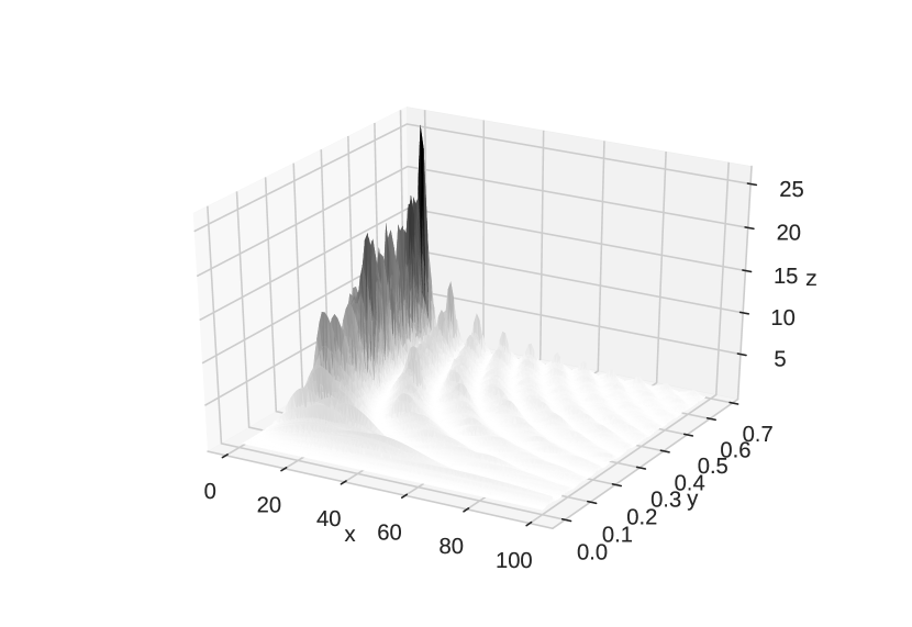
(a)

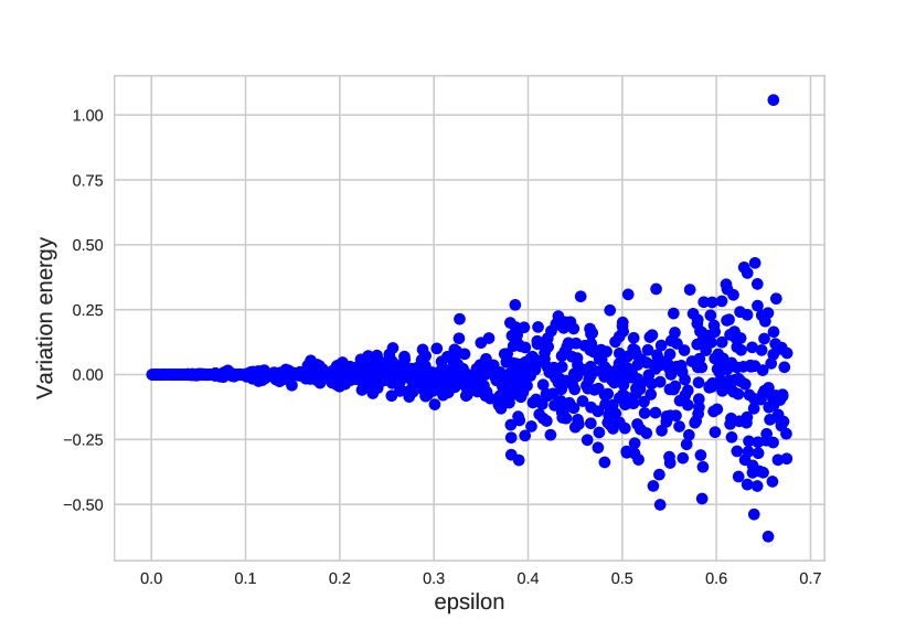
(b)

Figure 1: Tempering of a normal distribution to a shifted and correlated normal distribution in dimension 10 (see the example in Section 4.1 for more details). Left: The normalized and weighted squared jumping distance (z-axis) as a function of $\epsilon$ (y-axis) and $L$ (x-axis) for the temperature $0.008$. Right: Variation of the difference in energy $\Delta E$ as a function of $\epsilon$ for the same temperature. The values of $L$ are randomized. Based on an SMC sampler with an HMC kernel based on $N=1,024$ particles.

3.3.2 Construction of a random distribution for $(\epsilon,L)$

Algorithm 6 describes how we generate values for $(\epsilon,L)$ during the second stage of our pre-tuning procedure. In words, these values are sampled from the weighted empirical distribution that correspond to the $N$ values $(\hat{\epsilon}_{t}^{i},\hat{L}_{t}^{i})$ generated (uniformly) during the first stage, with weights given by performance metric (6). We visualize this metric as a function of $\epsilon,L$ in Figure 1(a).

Input: Resampled particles $\tilde{x}_{t-1}^{i}$, $i\in 1:N$, HMC flow $\widehat{\Phi}_{\cdot,\cdot}$ (targeting $\pi_{t-1}$), $\epsilon^{\star}_{t-1}$

Result: Sample of $(\epsilon^{i}_{t},L_{t}^{i})$, $i\in 1:N$, upper bound $\epsilon^{\star}_{t}$

1 foreach $i\in 1:N$ do

2       Sample $\hat{\epsilon}^{i}_{t}\sim\mathcal{U}[0,\epsilon^{\star}_{t-1}]$ and $\hat{L}^{i}_{t}\sim\mathcal{U}\{1:L_{max}\}$;

3       Sample $p_{t}^{i}\sim\mathcal{N}(0_{d},\mathbf{M}_{t-1})$;

4       Apply the leapfrog integration: $(\hat{p}^{i}_{t},\hat{x}^{i}_{t})\leftarrow\widehat{\Phi}_{\hat{\epsilon}^{i}_{t},\hat{L}^{i}_{t}}(p_{t}^{i},\tilde{x}_{t-1}^{i})$;

5       Calculate $\Delta E^{i}_{t}$ and $\tilde{\Lambda}(\tilde{x}_{t-1}^{i},\hat{x}^{i}_{t})$

6Calculate $\epsilon^{\star}_{t}$ based on the quantile regression of $\Delta E^{i}_{t}$ on $\hat{\epsilon}^{i}_{t}$ $\forall i\in 1:N$;

Sample $(\epsilon_{t}^{i},L_{t}^{i})\sim\mathcal{C}at\left(w^{i}_{t},\{\hat{\epsilon}^{i}_{t},\hat{L}^{i}_{t}\}\right)$, where $w^{i}_{t}\propto\tilde{\Lambda}(\tilde{x}_{t-1}^{i},\hat{x}^{i}_{t})$ $\forall i\in 1:N$;

Algorithm 6 (PR) Pre-tuning of the HMC kernel

3.3.3 Range of values for $L$

During the first stage of our pre-tuning procedure, $L$ is generated uniformly within range $[0,L_{\max}]$. The quantity $L_{\max}$ is initialized to some user-chosen value (we took $L_{\max}=100$ in our simulations). Whenever a large proportion of the $L_{t}^{i}$ generated by Algorithm 6 is close to $L_{\max}$, we increase $L_{\max}$ by a small amount (5 in our simulations). Similarly, whenever a large proportion of these values are far away from $L_{\max}$, we decrease $L_{\max}$ by the same small amount.

3.4 Discussion of the tuning procedures

Comparison of the two algorithms

The difference between the two procedures consists in the pre-tuning phase at each intermediate step of the sampler. On one hand, pre-tuning makes the SMC sampler more costly per intermediate step. On the other hand this approach makes the sampler more robust to a sudden change in the sequence of distributions. We illustrate this point in our numerical experiments.

Both of the suggested tuning procedures have computational costs linear in the number of particles $N$, in line with the other operations performed in the SMC sampler.

Other potential approaches to tuning HMC within SMC

One could try to maximize the squared jumping distance as a function of the position of every particle, based on the associated values of $(\epsilon,L)$. However, learning optimal parameters for every position might be challenging, possibly harder than the original Monte Carlo problem of interest. In line with Girolami and Calderhead, (2011) one could use a position dependent mass matrix that would take the geometry of the target space into account, for instance related to higher-order derivatives of the target probability density function.

Returning to the choice of $(\epsilon,L)$ one could use an approach based on Bayesian optimization (Snoek et al.,, 2012), based on the performance of the $(\epsilon_{t-1}^{i},L_{t-1}^{i})$ at the previous iteration. This idea would amount to a parallel version of Mohamed et al., (2013). However, it is not clear how this approach would behave if the underlying distributions evolve over time. Not using a pre-tuning step reduces the computational load at the expense of making the sampler potentially less robust. Moreover, the approach of Fearnhead and Taylor, (2013) already explores the hyperparameter space adaptively without requiring additional model specifications. If framed as a Bandit problem, fixing over time a grid of possible values $(\epsilon,L)$ could be problematic if the grid misses relevant parts of the hyperparameter space. This holds true in particular when using continuous Bayesian optimization, where one typically has to define some box constraints on the underlying space.

Extensions

The tuning procedure based on pre-tuning might also be used for tuning random walk (RW) Metropolis or MALA (Metropolis adjusted Langevin) kernels. In the first case we may use median regression to find an upper bound for the scale such that the acceptance rate is close to $23.4\%$ (Roberts et al.,, 1997). In the second case one may target an acceptance rate of $57.4\%$ (Roberts and Rosenthal,, 1998). (MALA kernels may be viewed as HMC kernels with $L=1$.) It recently came to our knowledge that the work of Salomone et al., (2018) also uses a pre-tuning approach for MCMC kernels within SMC samplers. A notable difference with our approach is that Salomone et al., (2018) concentrates on finding a single tuning parameter, rather than a distribution.

4 Experiments

Our experiments highlight the importance of adapting SMC samplers, in particular the parameters of their Markov kernels. Specifically, we try to answer the following questions. How important is it to adapt (a) the number of temperature steps and (b) the number of move steps? (c) Does our tuning procedure of HMC kernels provide reasonable values of $(\epsilon,L)$ compared to other tuning procedures of HMC? (d) To what extent does HMC within an SMC sampler scale with the dimension and may be applied to real data applications? (e) How robust are SMC samplers to multimodality?

For this purpose we compare adaptive (A) and non-adaptive (N) versions of HMC-based SMC samplers, where the adaptation may be carried out using either the FT approach (our variant of the approach of Fearnhead and Taylor,, 2013) or the PR (pre-tuning) approach. We also include in our comparison SMC samplers based on random walk (RW) and MALA kernels, and the FT adaptation procedure. We call our algorithms accordingly: i.e. HMCAFT stands for an SMC sampler using HMC kernels, which are adapted using the FT procedure.

In all the considered SMC samplers, the mass matrix $\mathbf{M}_{t}$ of the MCMC kernels is set to the diagonal of the covariance matrix obtained at the previous iteration. Unless otherwise stated, the number of particles is $N=1,024$ and the resampling is triggered when the ESS drops below $N/2$. The computational load of a given sampler is defined as the number of gradient evaluations, plus the number of likelihood evaluations. Note, that this is a conservative choice as computations of the likelihood and the gradient often involve the same computations. Most of our comparisons are in terms of adjusted variance, or adjusted MSE (mean squared error), by which we mean: variance (or MSE) times computational load.

All HMC-based samplers are initialized with uniform random draws of $\epsilon$ on $[0,0.1]$ and $L$ on $\{1,100\}$. The MALA and RW-based samplers are initialized with random draws of the scale parameter on $[0,1]$. The initial mass matrix is set to the identity for all different samplers. All samplers choose adaptively the number of move steps based on Algorithm 3. Code for reproducing the results shown below is available under https://github.com/alexanderbuchholz/hsmc.

4.1 Tempering from an isotropic Gaussian to a shifted correlated Gaussian

As a first toy example we consider a tempering sequence that starts at an isotropic Gaussian $\pi_{0}=\mathcal{N}(0_{d},I_{d})$, and finishes at a shifted and correlated Gaussian $\pi_{T}=\mathcal{N}(\mu,\Xi)$, where $\mu=2\times\mathbf{1}_{d}$, for different values of $d$. For the covariance we set the off-diagonal correlation to $0.7$ and the marginal variances to elements of the equally spaced sequence $\tilde{\Xi}=[0.1,\cdots,10]$. We get the covariance $\Xi=\operatorname{diag}\tilde{\Xi}^{1/2}\operatorname{corr}(X)\operatorname{diag}\tilde{\Xi}^{1/2}$. This toy example is rather challenging due to the different length scales of the variance, the correlation and the shifted mean of the target. In this example the true mean, variance and normalizing constants are available. Therefore we report the mean squared error (MSE) of the estimators. We use normalized importance weights and thus $Z_{T}/Z_{0}=1$.

We first compare the following SMC samplers: MALA, HMCAFT and HMCAPR (according to the denomination laid out in the previous section). We add to the comparison HMCNFT, an SMC sampler using adaptive (FT based) HMC steps, but where the sequence of temperatures is fixed a priori to a long equi-spaced sequence (the size of which is set according to the number of temperatures chosen adaptively during one run of HMCAFT).

Figure 2(a) plots the ESS as a function of the temperature, for dimension $d=500$, for algorithms HMCAFT and HMCNFT. Figures 2b and 3 compare the SMC samplers in terms of computational load (Figure 2b) and adjusted MSE (i.e. MSE times the computational load) for the normalizing constant and the expectation of the first component (with respect to the target). The results for other components (not shown here) are similar to the results for the first component.

A first observation is that it seems useful to adapt the sequence of temperatures: HMCNFT is outperformed by all the other algorithms for both estimates. A second observation is that there is no clear ranking between the three other samplers. HMC-based samplers (and particularly HMCAFT) do perform better than the MALA-based sampler for the normalizing constant, but the picture is less clear for the posterior expectation of the first component. It is remarkable that, even in dimensions as high as 500, MALA kernels may be competitive.

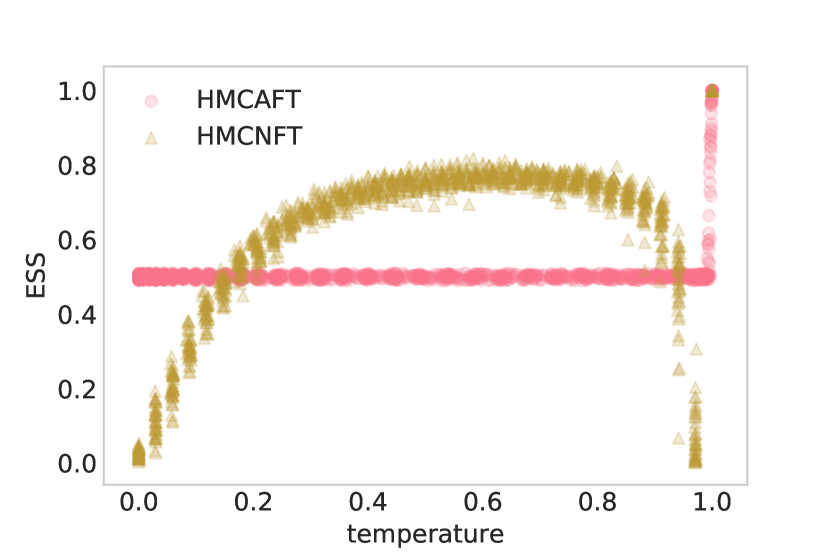
(a)

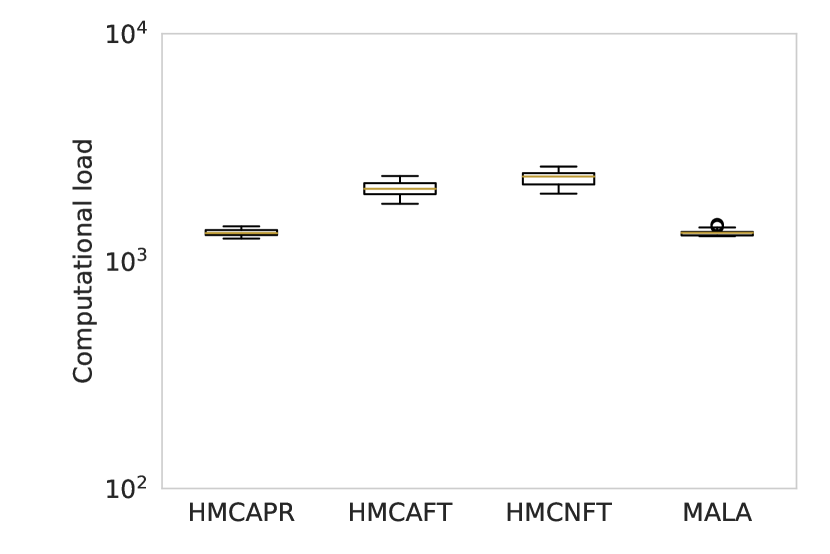
(b)

Figure 2: ESS and temperature steps in dimension $d=500$ (Figure 2(a)) and the computational load of the sampler in terms of the number of total gradient evaluations (Figure 2(b)).

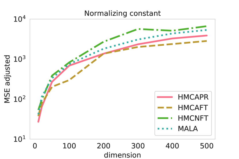
(a)

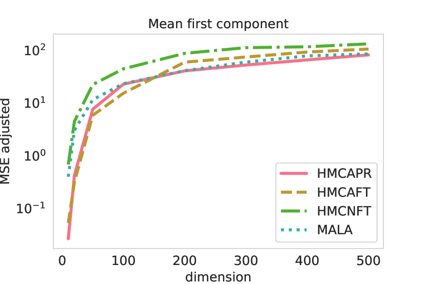
(b)

Figure 3: Mean squared error of the normalization constant (Figure 3(a)) and the mean squared error of the first component of the mean (Figure 3(b)) multiplied by the computational cost over dimensions. Based on $40$ repetitions of the samplers with $N=1,024$ particles.

In a second step, we compare the impact of adapting the number of move steps of the samplers. We restrict the comparison to a MALA-based sampler that uses FT tuning and an HMC-based sampler that uses PR tuning. For the non-adaptive samplers (N) the number of move steps is fixed to a constant number, equal to the average number of move steps over the complete run of an adaptive sampler. The temperatures are chosen adaptively.

We compare the performance of the samplers in estimating the trace of the variance $\Xi$. The results are shown in Figure 4(a) and the associated computational cost is shown in Figure 4(b). The adaptive samplers seem to offer a similar trade-off in terms of MSE versus computational load.

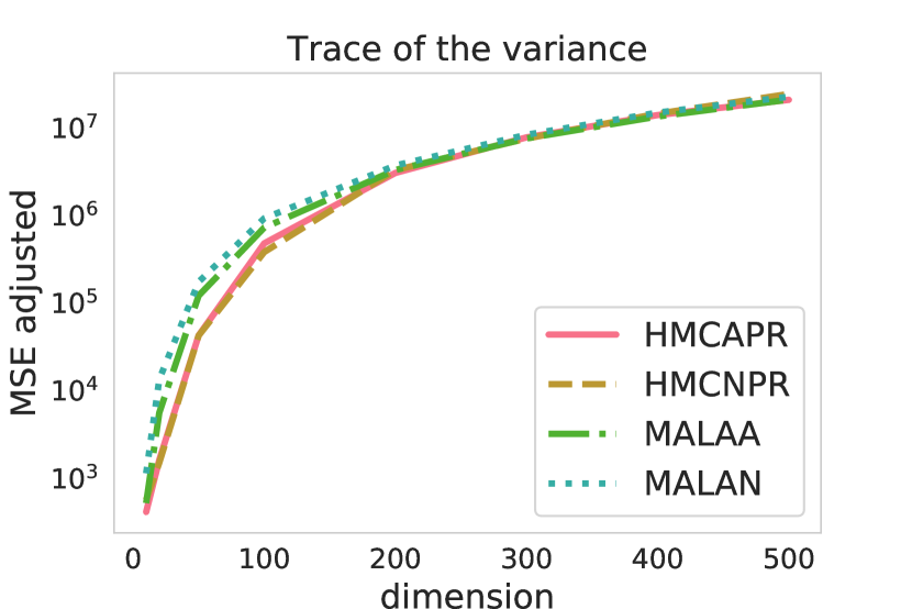
(a)

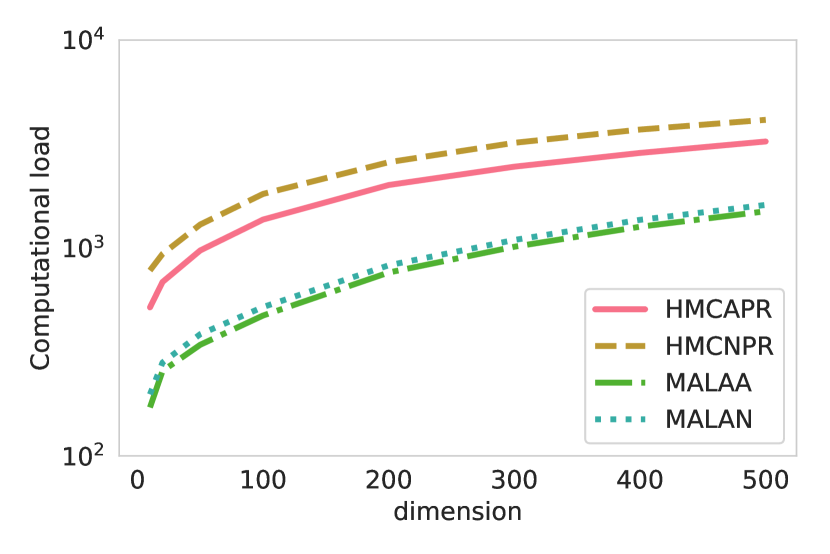
(b)

Figure 4: Mean squared error of the trace of the estimated variance (Figure 4(a)) multiplied by the computational cost (Figure 4(b)) over dimensions. Based on $40$ repetitions of the samplers with $N=1,024$ particles.

In order to assess the performance of the two tuning procedures (FT and PR), we compare the tuning parameters obtained at the final stage of our SMC samplers (HMCAFT and HMCAPR) with those obtained from the following MCMC procedures: NUTS (Hoffman and Gelman,, 2014) and the adaptive MCMC algorithm of Mohamed et al., (2013). NUTS iteratively tunes the mass matrix $\mathbf{M}$, the number of leapfrog steps $L$ and the step size $\epsilon$ in order to achieve a high ESJD (expected squared jumping distance). The adaptive HMC sampler of Mohamed et al., (2013) uses Bayesian optimization in order to find values of $(\epsilon,L)$ that yield a high ESJD.

For this purpose we run our HMC-based SMC samplers and record the achieved ESJD of the HMC kernel at the final distribution $\pi_{T}$. NUTS and the adaptive HMC sampler are run directly on the final target distribution. For NUTS we use the implementation available in STAN; for the adaptive HMC sampler we reimplemented the procedure of Mohamed et al., (2013). After the convergence of the tuning procedures we run the chain for $2,000$ iterations and discard a burnin of $1,000$ samples. The ESJD is calculated on the remaining $1,000$ iterations of the chain. The results of this comparison are shown in Table 1. We see that both the HMC-based SMC samplers, NUTS and the adaptive HMC tuning achieve an ESJD of the same order of magnitude. Thus, our tuning procedure gives values of $(\epsilon,L)$ that yield an ESJD comparable to other existing procedures.

Dimension	SMC HMCAPR	SMC HMCAFT	SMC MALA	NUTS	adaptive HMC
10	50.64	61.03	9.89	59.88	134.70
50	174.64	255.98	30.56	204.34	190.67
200	639.35	989.97	85.22	1,281.06	927.30
500	1,556.27	1,311.60	154.05	2,210.44	1,731.04

Table 1: Average squared jumping distance of different algorithms for the Gaussian target in the first example (based on 40 runs). The results are based on 1,024 samples for the SMC samplers. For the MCMC samplers (NUTS, adaptive HMC) we used a length of 2,000 states where the first 1,000 states are discarded as burn-in.

4.2 Tempering from a Gaussian to a mixture of two correlated Gaussians

The aim of our second example is to assess the robustness of SMC samplers with respect to multimodality. We temper from the prior $\pi_{0}=\mathcal{N}(\mu_{0},5I_{d})$ towards a mixture of shifted and correlated Gaussians $\pi_{T}=0.3\mathcal{N}(\mu,\Xi_{1})+0.7\mathcal{N}(-\mu,\Xi_{2})$, where $\mu=4\times\mathbf{1}_{d}$ and we set the off diagonal correlation to $0.7$ for $\Xi_{1}$ and to $0.1$ for $\Xi_{2}$. The variances are set to elements of the equally spaced sequence $\tilde{\Xi_{j}}=[1,\cdots,2]$ for $j=1,2$. The covariances $\Xi_{j}$ are based on the same formula as in the first example. In order to make the example more challenging we set $\mu_{0}=\mathbf{1}_{d}$. Thus, the starting point of the sampler is slightly biased towards one of the two modes. We evaluate the performance of the samplers by evaluating the signs of the particles and use therefore the statistic $T_{i}:=1/d\sum_{j=1}^{d}\mathds{1}_{\{\operatorname{sign}X_{j,i}=+1\}}$, based on a single particle. We expect a proportion of $30\%$ of the signs to be positive, i.e. $1/N\sum_{i=1}^{N}T_{i}\approx 0.3$, if the modes are correctly recovered. Our measure of error is based on the squared deviation from this value. We consider the following SMC samplers: MALA, RW, HMCAFT, and HMCAPR. All the samplers choose adaptively the number of move steps and the temperatures.

As shown by Figure 5(b) the two HMC-based samplers yield a lower error of the recovered modes adjusted for computation in moderate dimensions. In terms of the recovery of the modes all samplers behave comparably, see Figure 5(a). Nevertheless, as the dimension of the problem exceeds $20$ all samplers tend to concentrate on one single mode. This problem may be solved by initializing the sampler with a wider distribution. However, this approach relies on the knowledge of the location of the modes.

Consequently, SMC samplers are robust to multimodality only in small dimensions and care must be taken when using SMC samplers in this setting. That said, HMC-based samplers seem slightly more robust to multimodality; see e.g. results for $d=10$ in Figure 5(a). See also the recent work of Mangoubi et al., (2018) for the performance of HMC versus RWMH on multimodal targets.

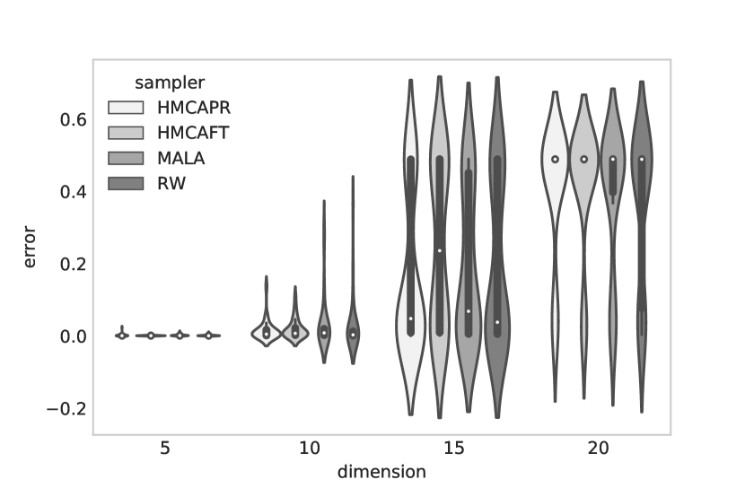
(a)

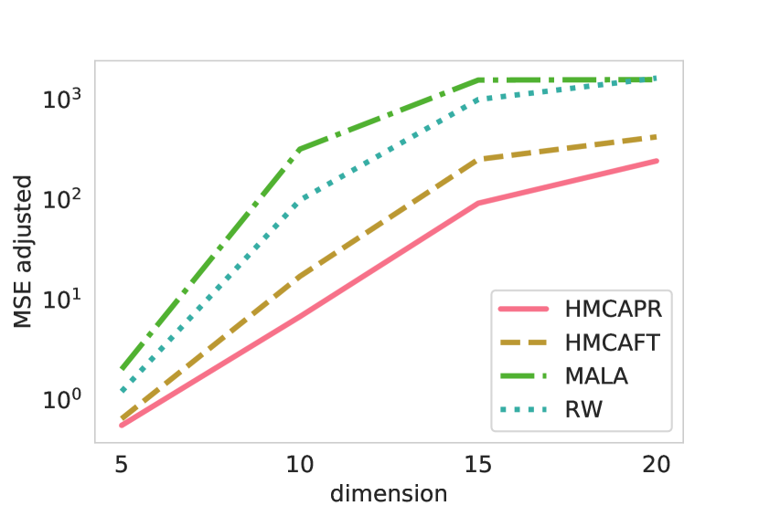
(b)

Figure 5: Left: Violinplot of the error, based on the squared difference of $1/N\sum_{i=1}^{N}T_{i}-0.3$. Right: Mean squared error of the proportion of recovered modes adjusted for the computation. Based on 40 runs of the samplers.

4.3 Tempering from an isotropic Student distribution to a shifted correlated Student distribution

As a different challenging toy example we study the tempering from an isotropic Student distribution $\pi_{0}=\mathcal{T}_{3}(0_{d},I_{d})$ with $3$ degrees of freedom towards a shifted and correlated Student distribution with $\nu=10$ degrees of freedom, i.e. $\pi_{T}=\mathcal{T}_{\nu}(\mu,\Xi)$. The mean and scale matrix are set as in the unimodal Gaussian example in 4.1.

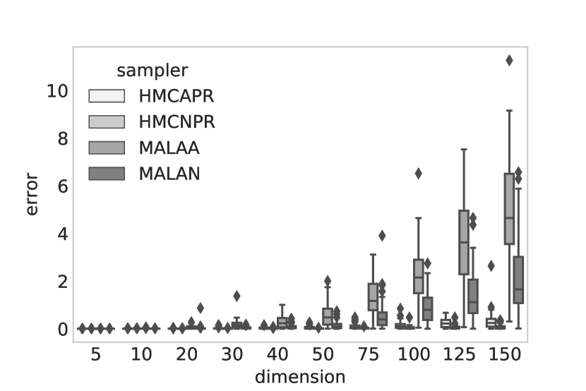
(a)

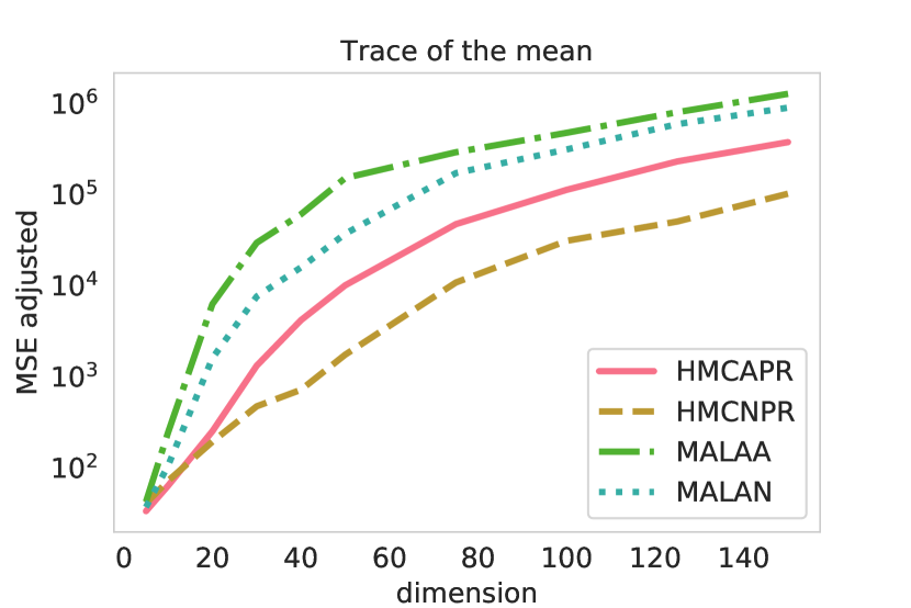
(b)

Figure 6: Figure 6(a) shows the squared error of the estimator of the normalizing constant. Figure 6(b) shows the squared error of the trace of the mean over different dimensions adjusted for computation. The results are based on $100$ runs of the samplers with $N=1,024$ particles.

This example is more challenging as the target distribution $\pi_{T}$ has heavy tails. We vary the dimension between $d=5$ and $d=150$. The temperature steps are chosen such that an ESS of $90\%$ is attained. The adaptive samplers (A) adjust the number of move steps according to Algorithm 3. For the non-adaptive samplers (N) the number of move steps is fixed to a constant number, equal to the average number of move steps over the complete run of an adaptive sampler. The temperatures are chosen adaptively. The MALA-based sampler uses FT tuning, the HMC-based sampler uses our pre-tuning (PR) approach.

The HMC-based samplers perform better when it comes to estimating the mean (see Figure 6(b)) and the normalizing constant (see Figure 6(a)). Both samplers based on a MALA kernel tend to work poorly in terms of the estimation of the normalizing constant when the dimension increases, see Figure 6(a).

In this particular example, we observe that the adaptation of the number of move steps has some negative impact on the performance of the samplers. We suspect that this is due to the heavy tails of the Student distribution: first, this phenomenon did not occur in our first numerical example, where the target had light tails (Gaussian); second, Livingstone et al., (2016) show that an HMC kernel cannot be geometrically ergodic when the target is heavy-tailed. Thus, setting the number of move steps to a fixed, large value may be beneficial for heavy-tailed targets. Our approach provides a guideline for finding this number.

4.4 Binary regression posterior

We now consider a Bayesian binary regression model. We observe $J$ vectors $z_{j}\in\mathbb{R}^{d}$ and $J$ outcomes $y_{j}\in\{0,1\}$. We assume $y_{j}\sim\mathcal{B}er(r(z_{j}^{T}\beta))$ where $r:\mathbb{R}\mapsto[0,1]$ is a link function. The parameter of interest is $\beta\in\mathbb{R}^{d}$, endowed with a Gaussian prior, i.e. $\beta\sim\mathcal{N}(0_{d},I_{d})$.

When using the logit link function $r:x\rightarrow\exp(-x)/(1+\exp(-x))$ we obtain a Bayesian logistic regression where the unnormalized log posterior is given as

$$\gamma(\beta)=\sum_{j=1}^{J}\left[(y_{j}-1)z_{j}^{T}\beta-\log(1+\exp(-z_{j}^{T}\beta)\right]-1/2\left\|\beta\right\|_{2}^{2}.$$

When using as link function the cumulative distribution function of a standard normal distribution, denoted $\Phi$, one obtains the Bayesian Probit regression. In this case the unnormalized log posterior is given as

$$\gamma(\beta)=\sum_{j=1}^{J}\left[y_{j}\log\Phi(z_{j}^{T}\beta)+(1-y_{j})\log(1-\Phi(z_{j}^{T}\beta))\right]-1/2\left\|\beta\right\|_{2}^{2}.$$

We set $\pi_{0}$ to a Gaussian approximation of the posterior obtained by Expectation Propagation (Minka,, 2001) as in Chopin and Ridgway, (2017).

We consider two datasets (both available in the UCI repository): sonar ($d=61$ covariates, $J=208$ observations) and musk ($d=95$, $J=476$, after removing a few covariates that are highly correlated with the rest). In both cases, an intercept is added, and the predictors are normalised (to have mean 0 and variance 1).

We compare the following SMC samplers: RW, MALA, HMCAFT, HMCAPR; see Figure 7 for the estimation of the marginal likelihoods (which may be used to perform model choice) and Figure 8 for the estimation of the posterior expectation of the first component. The results for other components (not shown here) are similar to the results for the first component. For all samplers we adapt the number of move steps and the temperature steps.

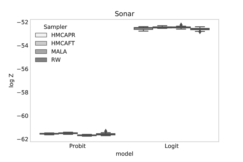
(a)

(b)

Figure 7: Normalization constants obtained for the probit and logit regression based on $40$ runs of the samplers. Figure 7(a) corresponds to the normalization constants obtained for the sonar dataset. The posterior has 61 dimensions. Figure 7(b) corresponds to the musk dataset. The posterior has 95 dimensions.

The four samplers perform similarly on on the sonar dataset, while they perform quite differently on the musk dataset. In the latter case, the MALA-based and RW-based samplers did not complete after 48 hours of running, so we had to remove them from the comparison. (In contrast, the two HMC-based samplers took less than 45 minutes to complete). In addition, FT adaptation leads to a high variance for the normalising constant.

Table 2 reports the logarithm of the adjusted variances for the four considered samplers, the two considered datasets, the two considered models (logit and probit) and a varying number of particles for the sonar dataset. By and large, HMCAPR seems the most robust approach; it often gives either the smallest, or a value close to the smallest, of the adjusted variances.

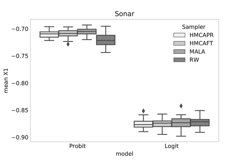
(a)

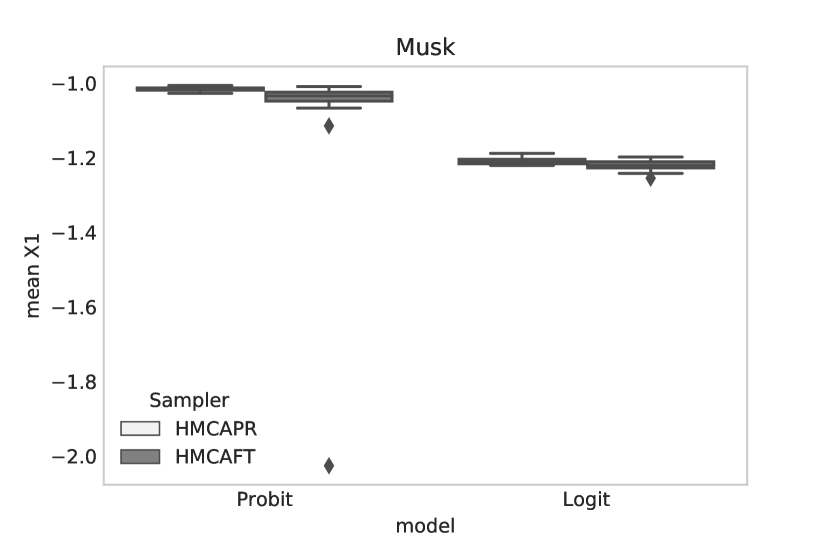
(b)

Figure 8: Estimated mean of the first component of the posterior obtained for the probit and logit regression. Figure 8(a) corresponds to the sonar dataset. Figure 8(b) corresponds to the musk dataset.

		Normalizing constant
		Logit				Probit
Dataset	Dim	HMCAPR	HMCAFT	MALA	RW	HMCAPR	HMCAFT	MALA	RW
Sonar, $N=2^{10}$	61	4.183	3.489	5.776	6.459	3.315	2.98	5.915	6.081
Sonar, $N=2^{13}$	61	2.685	2.233	4.384	5.362	2.788	3.686	4.883	5.285
Musk	95	6.09	11.519	-	-	6.596	8.62	-	-
		Mean first component
		Logit				Probit
Dataset	Dim	HMCAPR	HMCAFT	MALA	RW	HMCAPR	HMCAFT	MALA	RW
Sonar, $N=2^{10}$	61	-3.409	-3.644	-0.978	-0.875	-3.86	-3.842	-1.706	-0.604
Sonar, $N=2^{13}$	61	-5.482	-5.792	-3.668	-3.255	-5.688	-3.346	-3.413	-2.961
Musk	95	-1.643	-1.147	-	-	-0.633	0.014	-	-

Table 2: Inefficiency of the estimation of the normalizing constant and the mean of the first component based on $40$ runs of the different samplers. Smaller is better. The inefficiency is measured as the log of the adjusted variances of the samplers (variance multiplied by the mean number of gradient and likelihood evaluations). For the RWMH sampler we adjust by the number of likelihood evaluations only. The best performing sampler for a particular model and number of particles is highlighted in bold.

4.5 Log Gaussian Cox model

In order to illustrate the advantage of HMC-based SMC samplers in high dimensions we consider the log Gaussian Cox point process model in Girolami and Calderhead, (2011), applied to the Finnish pine saplings dataset. This dataset consists of the geographic position of 126 trees. The aim is to recover the latent process $X\in\mathbb{R}^{d\times d}$ from the realization of a Poisson process $Y=(y_{j,k})_{j,k}$ with intensity $m\Lambda(j,k)=m\exp(x_{j,k})$, where $m=1/d^{2}$ and $X=(x_{j,k})_{j,k}$ is a Gaussian process with mean $\mathbb{E}\left[X\right]=\mu\times\mathbf{1}_{d\times d}$ and covariance function $\Sigma_{(j,k)(j^{\prime},k^{\prime})}=\sigma^{2}\exp(-\delta(j,j^{\prime},k,k^{\prime})/(d\beta))$, where $\delta(j,j^{\prime},k,k^{\prime})=\sqrt{(j-j^{\prime})^{2}+(k-k^{\prime})^{2}}$.

The posterior density of the model is given as

$$p(x|y,\mu,\sigma^{2},\beta)\propto\left\{\prod_{j,k}^{d}\exp(y_{j,k}x_{j,k}-m\exp(x_{j,k}))\right\}\times\exp\left\{-1/2(x-\mu)^{T}\Sigma^{-1}(x-\mu)\right\},$$

where the second factor is the Gaussian prior density.

Following the results of Christensen et al., (2005) we fix $\beta=1/33$, $\sigma^{2}=1.91$ and $\mu=\log(126)-\sigma^{2}/2$. We vary the dimension of the problem from $d=100$ to $d=16,384$ by considering different discretizations. We consider three SMC samplers: MALA, HMCAFT and HMCAPR. The starting distribution is the prior.

Figure 9(b) shows that the HMC-based samplers estimate well the normalizing constant, even for a large dimension $d$. Moreover, we estimate the cumulative mean throughout different dimensions with relatively low variance, see Figure 9(a). We omitted the simulation for the MALA-based samplers, as the simulation took excessively long in dimension $4,096$ due to slow mixing of the kernel. The estimated posterior mean of the latent field for dimension $900$ is plotted in Figure 9(c).

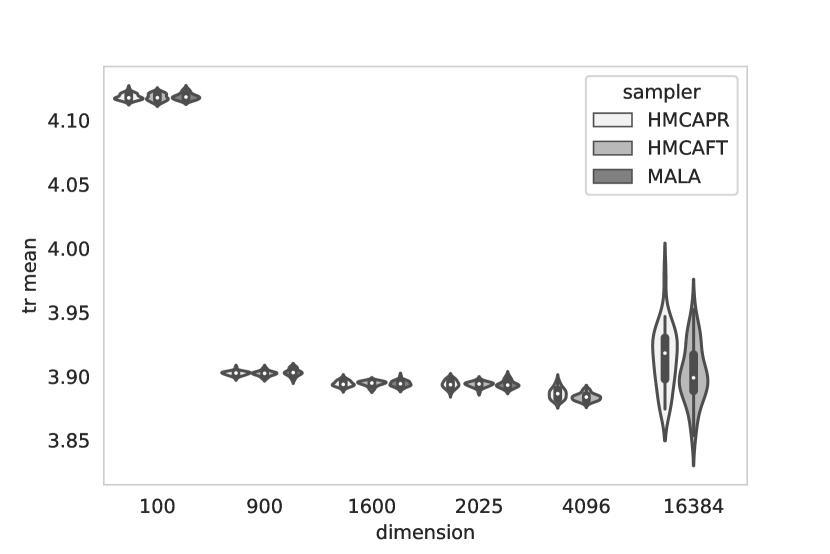
(a)

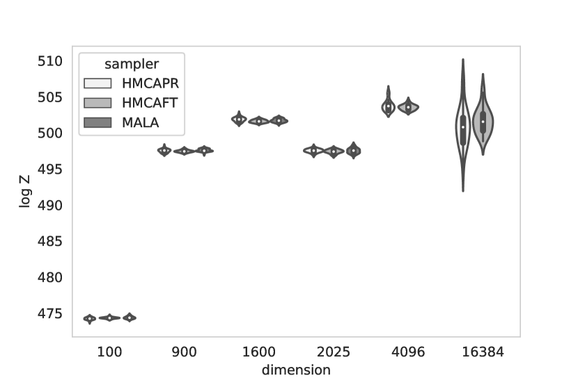
(b)

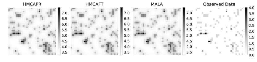
(c)

Figure 9: Tempering from a normal prior to the posterior of log Gaussian Cox process over various dimensions. Figure 9(a) illustrates the estimations of the normalizing constants. Figure 9(b) illustrates the estimated cumulative posterior mean. Figure 9(c) illustrates the recovered componentwise posterior mean of the process in dimension $900$.

Table 3 reports adjusted variances (variances times computational load) for the considered SMC samplers. We see that the MALA-based sampler is not competitive when the dimension increases. Regarding the adaptation scheme, FT outperforms PR, especially in high dimension.

	Normalizing constant			Mean first component
Dim	HMCAPR	HMCAFT	MALA	HMCAPR	HMCAFT	MALA
100	2.292	2.03	2.933	-6.4	-5.613	-5.559
400	3.296	2.255	3.812	-5.895	-5.913	-4.765
900	3.89	2.776	4.373	-6.192	-6.141	-4.276
1,600	4.735	3.226	5.224	-5.217	-6.046	-4.162
2,500	4.5	4.072	6.246	-4.405	-5.636	-3.476
4,096	7.055	5.071	-	-3.2	-4.701	-
16,384	10.002	8.864	-	0.538	0.142	-

Table 3: Inefficiency of the estimation of the normalizing constant and the mean of the first component based on $40$ runs of the different samplers. The inefficiency is measured as the log of adjusted variances of the samplers (variance multiplied by the mean number of gradient and likelihood evaluations). Smaller is better.

5 Discussion

Our experiments indicate that the relative performance of HMC kernels within SMC depends on the dimension of the problem. For low to medium dimensions, RW and MALA are much faster, and tend to perform reasonably well. On the other hand, for high dimensions, HMC kernels outperform, sometimes significantly, RW and MALA kernels.

The key to good performance of SMC samplers (based on HMC or other kernels) is to adaptively tune the Markov kernels used in the propagation step. We have considered two approaches in this paper. On posterior distributions with reasonable correlation our adaption of the approach by Fearnhead and Taylor, (2013) works best. Our approach based on pre-tuning of the HMC kernels is more robust to changes in the subsequent target distributions, as illustrated by our binary regression example. This holds in particular when using SMC samplers for model choice. Moreover, we showed that, when sensibly tuned, SMC samplers with HMC kernels can scale to high dimensional problems. From a practical point of view and if the structure of the posterior is unknown the second approach may be the more prudent choice.

All in all, our methodology provides a principled approach for an automatic adaption of SMC samplers, applicable over a range of various models in different dimensions.

References

- Agapiou et al., (2017) Agapiou, S., Papaspiliopoulos, O., Sanz-Alonso, D., Stuart, A., et al. (2017). Importance sampling: Intrinsic dimension and computational cost. Statistical Science, 32(3):405–431.
- Andrieu and Thoms, (2008) Andrieu, C. and Thoms, J. (2008). A tutorial on adaptive MCMC. Statistics and computing, 18(4):343–373.
- Beskos et al., (2016) Beskos, A., Jasra, A., Kantas, N., and Thiery, A. (2016). On the convergence of adaptive sequential Monte Carlo methods. The Annals of Applied Probability, 26(2):1111–1146.
- Beskos et al., (2013) Beskos, A., Pillai, N., Roberts, G., Sanz-Serna, J.-M., and Stuart, A. (2013). Optimal tuning of the hybrid Monte Carlo algorithm. Bernoulli, 19(5A):1501–1534.
- Betancourt, (2016) Betancourt, M. (2016). Identifying the optimal integration time in Hamiltonian Monte Carlo. arXiv preprint arXiv:1601.00225.
- Betancourt et al., (2014) Betancourt, M., Byrne, S., and Girolami, M. (2014). Optimizing the integrator step size for Hamiltonian Monte Carlo. arXiv preprint arXiv:1411.6669.
- Bou-Rabee and Sanz-Serna, (2018) Bou-Rabee, N. and Sanz-Serna, J. M. (2018). Geometric integrators and the Hamiltonian Monte Carlo method. Acta Numerica, 27:113–206.
- Burda and Daviet, (2018) Burda, M. and Daviet, R. (2018). Hamiltonian Sequential Monte Carlo with Application to Consumer Choice Behavior. Working Papers tecipa-618, University of Toronto, Department of Economics.
- Carpenter et al., (2017) Carpenter, B., Gelman, A., Hoffman, M., Lee, D., Goodrich, B., Betancourt, M., Brubaker, M., Guo, J., Li, P., and Riddell, A. (2017). Stan: A Probabilistic Programming Language. Journal of Statistical Software, Articles, 76(1):1–32.
- Chopin, (2002) Chopin, N. (2002). A sequential particle filter method for static models. Biometrika, 89(3):539–552.
- Chopin and Ridgway, (2017) Chopin, N. and Ridgway, J. (2017). Leave Pima Indians alone: binary regression as a benchmark for Bayesian computation. Statistical Science, 32(1):64–87.
- Chopin et al., (2013) Chopin, N., Rousseau, J., and Liseo, B. (2013). Computational aspects of Bayesian spectral density estimation. Journal of Computational and Graphical Statistics, 22(3):533–557.
- Christensen et al., (2005) Christensen, O. F., Roberts, G. O., and Rosenthal, J. S. (2005). Scaling limits for the transient phase of local Metropolis–Hastings algorithms. Journal of the Royal Statistical Society: Series B (Statistical Methodology), 67(2):253–268.
- Creutz, (1988) Creutz, M. (1988). Global Monte Carlo algorithms for many-fermion systems. Physical Review D, 38(4):1228.
- Daviet, (2018) Daviet, R. (2018). Inference with Hamiltonian Sequential Monte Carlo Simulators. arXiv preprint arXiv:1812.07978.
- Del Moral et al., (2006) Del Moral, P., Doucet, A., and Jasra, A. (2006). Sequential Monte Carlo samplers. Journal of the Royal Statistical Society: Series B (Statistical Methodology), 68(3):411–436.
- Del Moral et al., (2007) Del Moral, P., Doucet, A., and Jasra, A. (2007). Sequential Monte Carlo for Bayesian Computation. Bayesian Statistics, (8):1–34.
- Duane et al., (1987) Duane, S., Kennedy, A. D., Pendleton, B. J., and Roweth, D. (1987). Hybrid Monte Carlo. Physics letters B, 195(2):216–222.