Near-threshold bound states of the dipole-dipole interaction

Abstract

We study the two-body bound states of a model Hamiltonian that describes the interaction between two field-oriented dipole moments. This model has been used extensively in many-body physics of ultracold polar molecules and magnetic atoms, but its few-body physics has been explored less fully. With a hard-wall short-range boundary condition, the dipole-dipole bound states are universal and exhibit a complicated pattern of avoided crossings between states of different character. For more realistic Lennard-Jones short-range interactions, we consider parameters representative of magnetic atoms and polar molecules. For magnetic atoms, the bound states are dominated by the Lennard-Jones potential, and the perturbative dipole-dipole interaction is suppressed by the special structure of van der Waals bound states. For polar molecules, we find a dense manifold of dipole-dipole bound states with many avoided crossings as a function of induced dipole or applied field, similar to those for hard-wall boundary conditions. This universal pattern of states may be observable spectroscopically for pairs of ultracold polar molecules.

I Introduction

The dipole-dipole interaction has been studied extensively in the many-body physics of ultracold polar molecules and magnetic atoms Micheli et al. (2006); Baranov (2008); Lahaye et al. (2009); Baranov et al. (2012). It is a long-range, anisotropic interaction that leads to a range of unique and exotic phenomena: new quantum phases of matter Astrakharchik et al. (2007); Büchler et al. (2007); Cooper and Shlyapnikov (2009); Capogrosso-Sansone et al. (2010); Macia et al. (2012), quantum magnetism Barnett et al. (2006); Gorshkov et al. (2011); Yan et al. (2013); Zou et al. (2017), and the anisotropic collapse of dipolar Bose-Einstein condensates Lahaye et al. (2008). Dipolar interactions also have applications in quantum computing DeMille (2002); Lukin et al. (2001); Yelin et al. (2006), and in quantum simulation Santos et al. (2004); Büchler et al. (2005); Jaksch and Zoller (2005).

Numerous species with significant dipole moments have now been created at ultracold temperatures. These include both high-spin magnetic atoms Griesmaier et al. (2005); Beaufils et al. (2008); Lu et al. (2011); Pasquiou et al. (2012); Aikawa et al. (2012), and polar molecules Ni et al. (2008); Takekoshi et al. (2014); Molony et al. (2014); Park et al. (2015); Guo et al. (2016); Truppe et al. (2017); Rvachov et al. (2017); McCarron et al. (2018). Before exploring the diverse many-body physics experimentally, we need to understand the 2-body physics, both ultracold scattering above threshold and weakly bound states below threshold.

The simplest model of the dipole-dipole interaction is that between two dipoles constrained to be parallel to one another. This model has been used extensively in many-body physics, but its two-body properties have been studied less fully. Bohn, Cavagnero and Ticknor (BCT) Ticknor (2008); Bohn et al. (2009) have used this model for the scattering of two dipoles with orientations fixed in space. They investigated the low-energy and high-energy regimes, using the Born and eikonal approximations, respectively. The Born approximation leads to an energy-independent cross section that scales with the fourth power of the induced dipole moment. This accounts for all partial waves except for pure $s$-wave scattering, which requires an additional term involving the scattering length. Since the scattering length diverges at resonances that occur when bound states cross threshold, it is important to characterize the bound states supported by the dipole-dipole interaction. These states may also be accessible spectroscopically.

In this paper, we investigate the bound states of a simple dipolar Hamiltonian. Section II describes the Hamiltonian and the approach used to compute bound states in the remainder of the paper. Section III describes the adiabatic potential curves produced by this Hamiltonian, and estimates the number of bound states supported by these curves semiclassically. Section IV discusses the bound states supported by the dipole-dipole Hamiltonian with hard-wall short-range boundary conditions. Section V employs a more realistic Lennard-Jones short-range interaction and discusses the bound states for two sets of parameters, representative of magnetic atoms and polar molecules, respectively.

II Hamiltonian

The Schrödinger equation considered by BCT Bohn et al. (2009) is

$$\left[-\frac{\hbar^{2}}{2M}\nabla^{2}+\hat{V}_{\mathrm{dip}}(\bm{R})+V_{\mathrm{SR}}(R)\right]\psi=E\psi.$$ (1)

Here, $M$ is the reduced mass, $V_{\mathrm{SR}}(R)$ is a short-range interaction, and

$$\hat{V}_{\mathrm{dip}}(\bm{R})=-\frac{2d_{1}d_{2}}{4\pi\epsilon_{0}}\frac{P_{2}(\cos\theta)}{R^{3}}$$ (2)

is the anisotropic dipole-dipole interaction. This Hamiltonian describes the interaction of two electric dipole moments, of magnitude $d_{1}$ and $d_{2}$, with fixed orientations in space. This commonly arises when both dipoles are oriented along the same space-fixed field. The distance between the dipole moments is $R$ and the angle between the interdipole axis and the external field axis is $\theta$. The interaction between two magnetic dipoles $\mu$ also follows Eq. 2 if expressed in terms of effective electric dipoles $d=\mu/c$, where $c$ is the speed of light.

Conceptually, the long-range dipole-dipole and short-range interactions act on different length scales. The short-range interaction may be viewed as defining a boundary condition for the pure dipole-dipole problem, obtained by dropping $V_{\mathrm{SR}}(R)$. The dipole-dipole part of the Schrödinger equation can then be brought into dimensionless form Ticknor (2008); Bohn et al. (2009)

$$\left[-\frac{1}{2}\frac{d^{2}}{dr^{2}}+\frac{\hat{L}^{2}}{2r^{2}}-\frac{2P_{2}(\cos\theta)}{r^{3}}\right]\psi=\varepsilon\psi,$$ (3)

where $r=R/R_{\mathrm{dip}}$, $\varepsilon=E/E_{\mathrm{dip}}$, and the dipole length and dipole energy are defined Bohn et al. (2009) as

$$R_{\mathrm{dip}} =\frac{Md_{1}d_{2}}{\hbar^{2}4\pi\epsilon_{0}},$$

$$E_{\mathrm{dip}} =\frac{\hbar^{2}}{MR_{\mathrm{dip}}^{2}}=\frac{\hbar^{6}(4\pi\epsilon_{0})^{2}}{M^{3}d_{1}^{2}d_{2}^{2}}.$$ (4)

It should be stressed that the dipole energy defined by Eq. 4 is not a measure of the dipole-dipole interaction energy, as the name may suggest. In fact, the dipole energy decreases as the dipole moment increases, whereas the strength of the dipole-dipole interaction increases. Because of this, the set of dipole-dipole bound states becomes more dense as the dipole moment increases.

The dimensionless Schrödinger equation, Eq. (3), leads to dynamics that is universal in the sense that it may be scaled for the parameters of any particular system Bohn et al. (2009) and depends only on a short-range boundary condition. In ultracold scattering, many systems follow a stronger form of universality, where scaled properties depend only on the $s$-wave scattering length Braaten and Hammer (2006), with no further dependence on different boundary conditions that generate the same scattering length. However, the dipole-dipole interaction is anisotropic and couples different partial waves. The dynamics thus depends on multiple partial waves, which may not exhibit the same periodicity with s-wave scattering length. Dipole-dipole systems thus do not follow the stronger form of universality.

Here, we model the short-range interaction or boundary condition in two different ways. First, we consider a hard-wall boundary condition and explore the near-threshold bound states as a function of the hard-wall position. This constitutes the simplest model of dipole-dipole interactions. Secondly, we include a Lennard-Jones short-range potential, which can model van der Waals attraction and short-range repulsion more physically. In particular, this introduces correlations between the short-range phases for different partial waves more physically than placing a hard wall at identical separations for all partial waves.

II.1 Computational Methods

We perform coupled-channels calculations to obtain bound states, using the bound computer code Hutson (2011). The nuclear wave function is expanded in partial waves, represented by the spherical harmonics $Y_{LM_{L}}(\theta,\phi)$. These are coupled by the dipole-dipole interaction, with matrix elements Brink and Satchler (1994)

$$\left\langle LM_{L}\left|\frac{-2P_{2}(\cos\theta)}{r^{3}}\right|L^{\prime}M^{\prime}_{L}\right\rangle=-2r^{-3}(-1)^{M_{L}^{\prime}}$$ (5)

$$\times\sqrt{(2L+1)(2L^{\prime}+1)}\begin{pmatrix}L&2&L^{\prime}\\ -M_{L}&0&M_{L}^{\prime}\end{pmatrix}\begin{pmatrix}L&2&L^{\prime}\\ 0&0&0\end{pmatrix},$$

which is non-zero only if $M_{L}=M_{L}^{\prime}$ and $|L-L^{\prime}|=2$ or 0 (but not if $L=L^{\prime}=0$). We mainly consider the case $M_{L}=0$ for even $L$, for which the $s$-wave $L=0$ channel occurs.

The solution of the coupled equations is propagated in two steps. The diabatic modified log-derivative propagator of Manolopoulos Manolopoulos (1986) is used outwards on an equidistant grid of spacing $\Delta R=10^{-5}R_{\mathrm{dip}}$ from $R_{\mathrm{min}}$ to $R_{\mathrm{mid}}=0.2R_{\mathrm{dip}}$. The Airy propagator of Alexander and Manolopoulos Alexander and Manolopoulos (1987) is used to propagate inwards from $R_{\mathrm{max}}=3R_{\mathrm{dip}}$ to $R_{\mathrm{mid}}$ using a radial grid with variable step size. The boundary conditions are such that the wave function vanishes at $R_{\mathrm{min}}$ and follows a Wentzel-Kramers-Brillouin (WKB) form at $R_{\mathrm{max}}$. At the matching point, $R_{\mathrm{match}}$, bound states are found by locating a zero in an eigenvalue of the matching matrix, i.e., the difference of incoming and outgoing log-derivative matrices, as a function of energy Hutson (1994). The matching point does not coincide with $R_{\mathrm{mid}}$, but is chosen at shorter separation to ensure that the matching is performed in the classically allowed region. In the case of hard-wall boundary conditions, the matching point is chosen as $R_{\mathrm{match}}=R_{\mathrm{min}}+10^{-3}R_{\mathrm{dip}}$, and otherwise we use $R_{\mathrm{match}}=8\leavevmode\nobreak\ a_{0}$, which is close to the minimum of the Lennard-Jones potential.

III Adiabatic potential curves

First, we consider the adiabatic potential curves (adiabats) of the reduced Hamiltonian in Eq. 3. The adiabats $\varepsilon_{n}^{\rm ad}(r)$ are defined as the eigenvalues of

$$\frac{\hat{L}^{2}}{2r^{2}}-\frac{2P_{2}(\cos\theta)}{r^{3}}$$ (6)

for fixed $r=R/R_{\mathrm{dip}}$. For $r\gg 1$, the centrifugal term dominates the dipole-dipole interaction, and the adiabatic states correspond to spherical harmonics $Y_{LM_{L}}(\theta,\phi)$. The lowest adiabat corresponds asymptotically to $L=0$ and has a vanishing first-order dipole-dipole interaction. Dipole-dipole coupling to the $L=2$ channel yields the second-order energy

$$\varepsilon^{(2)}_{L=0}(r) =-\frac{r^{2}}{3}\left|\left\langle 00\left|\frac{2P_{2}(\cos\theta)}{r^{3}}\right|20\right\rangle\right|^{2}$$

$$=-\frac{4}{15}r^{-4}.$$ (7)

The lowest adiabat thus varies asymptotically as $-C_{4}R^{-4}$. We can define a corresponding length scale as

$$R_{4}=\sqrt{\frac{2MC_{4}}{\hbar^{2}}}=\sqrt{\frac{8}{15}}R_{\mathrm{dip}}\approx 0.73R_{\mathrm{dip}}.$$ (8)

This differs slightly from the value 1.09 $R_{\mathrm{dip}}$ given in Ref. Bohn et al., 2009. In the opposite limit, where the dipole-dipole interaction dominates, the lowest adiabat is simply $-2r^{-3}$ and the corresponding eigenstate is localized completely at $\theta=0$ and $\pi$, where the dipoles lie head-to-tail along the field direction.

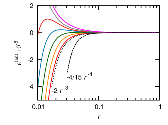
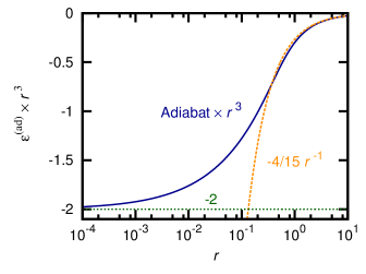
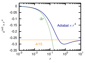
Figure 1: Top: Low-lying adiabats of the BCT Hamiltonian, Eq. (3), for even $L$ and $M_{L}=0$. Middle and bottom: Lowest adiabat multiplied by $r^{3}$ and $r^{4}$ respectively. Short-range and long-range approximations to the lowest adiabat, $-2r^{-3}$ and $-4/15r^{-4}$, respectively, are also included.

The calculated adiabats are shown in Fig. 1. The lower two panels of this figure show the lowest adiabat multiplied by $r^{3}$ and $r^{4}$, and show how it approaches the short-range and long-range limits $-2r^{-3}$ and $-4/15r^{-4}$. There is clearly an extended region for intermediate $r$ where neither approximation is accurate. The long-range $r^{-4}$ form is accurate only for $r>10$. Therefore, this form is appropriate for describing states only if they are bound by a small fraction of the dipole energy; in many cases there are no such states. This contrasts with other long-range interactions, such as the $R^{-6}$ interaction between neutral atoms, which often remain appropriate at depths of hundreds to thousands of times their corresponding energy scale. When $r$ is of order unity, the dipole-dipole coupling and centrifugal terms are roughly comparable. This leads to nonadiabatic coupling as the eigenstates change with $r$ from freely orbiting to states localized in $\theta$ by the dipole-dipole potential. Describing the states in a partial-wave expansion requires inclusion of functions with increasing values of $L$ as $r$ decreases. The change in character takes place over an extended range of $r$, as the relative strength of the two terms depends only linearly on $r$.

Higher-$L$ adiabats are repulsive at long range, and have centrifugal barriers that move inwards and increase in height with increasing $L$. Outside the barrier, the potentials are dominated by the centrifugal term. Inside the barrier, the dipole-dipole interaction dominates; eventually the eigenstates again localize in $\theta$, leading to adiabatic potentials proportional to $r^{-3}$.

III.1 WKB estimate of the number of bound states

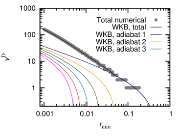
Figure 2: The total number of states obtained from coupled-channels calculations compared to the semi-classical WKB result.

In this section, we estimate the number of bound states supported by each adiabat semiclassically. To this end, we compute the phase integral at zero energy

$$\Phi_{n}(r_{\mathrm{min}})=\int_{r_{\mathrm{min}}}^{\infty}\Re\left(\sqrt{2\varepsilon_{n}^{\rm ad}(r)}\right)dr,$$ (9)

for each adiabat. Taking the real part of the integrand ensures that only the classically allowed region contributes. The WKB quantization condition is used to define a non-integer quantum number at dissociation, i.e., at zero energy,

$$v^{\rm D}_{n}(r_{\mathrm{min}})=\frac{\Phi_{n}(r_{\mathrm{min}})}{\pi}-\frac{1}{2}$$ (10)

which serves to estimate the total number of bound states.

Estimated numbers of bound states for different adiabats, and the total number of bound states, are shown in Fig. 2. The multichannel node count Johnson (1978) at zero energy from coupled-channels calculations is also shown for comparison. As $r_{\mathrm{min}}$ is decreased, the number of bound states supported by the lowest adiabat increases rapidly. Furthermore, excited adiabats start to contribute bound states as $r_{\mathrm{min}}$ is decreased to include the negative-energy regions of these adiabats, inside their long-range centrifugal barriers. The first states appear with $r_{\mathrm{min}}$ of order 0.1, and it can be seen from Fig. 1 that in this region the lowest adiabat has deviated substantially from its $r^{-4}$ long-range form. Therefore, for our purposes, it is clearly insufficient to approximate the energy of the lowest adiabat by its long-range form. For $r_{\mathrm{min}}\ll 0.1$, the adiabatic states localize in $\theta$ as the $r^{-3}$ dipole-dipole interaction dominates, and the number of states supported by each adiabat approaches the corresponding power-law dependence $v^{\rm D}_{n}\propto r_{\mathrm{min}}^{-1/2}$. The total number of bound states rises as a higher inverse power than the number in the individual adiabats as the number of contributing adiabats also rises rapidly as $r_{\mathrm{min}}$ decreases.

IV Hard-wall boundary condition

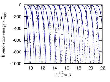
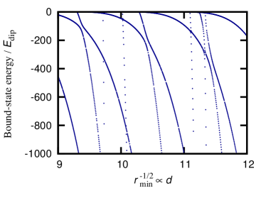
Figure 3: Bound states as a function of $r_{\mathrm{min}}^{-1/2}$, which is proportional to the dipole moment for fixed short-range boundary condition.

We calculate dipole-dipole bound states as a function of the position of the hard-wall short-range boundary condition, $R_{\mathrm{min}}$. These calculations use coupled-channel calculations as described in section II.1, and do not make an adiabatic separation. The bound-state energies are universal functions of $r_{\mathrm{min}}=R_{\mathrm{min}}/R_{\mathrm{dip}}$. They are shown in Fig. 3 as a function of $r_{\mathrm{min}}^{-1/2}$, which is proportional to the dipole moment for fixed $R_{\mathrm{min}}$. This figure can therefore be viewed as showing bound states as a function of the dipole moment. It corresponds to the way that polar molecules could be controlled by varying an applied electric field: The short-range boundary condition is fixed by the short-range potential, while the induced dipole moment varies with field. There is a regular series of states tending relatively slowly towards threshold, which will create broad resonances in the s-wave dipolar scattering Ticknor and Bohn (2005). These are crossed by steeper states which will create additional narrower resonances.

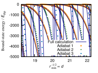
Figure 4: Bound states as a function of $r_{\mathrm{min}}^{-1/2}$, both from adiabatic and full coupled-channels calculations.

Bound states calculated in the adiabatic approximation are compared to the full calculation in Fig. 4. The adiabatic calculations agree well with the coupled channels calculations except near avoided crossings, demonstrating that the dynamics is mostly adiabatic. The steeper states are supported by excited adiabats, which have increasingly high barriers at large interdipole distances that confine the wavefunction to relatively short range and increase the vibrational spacing at threshold. This explains the difference in dependence on and periodicity with $r_{\mathrm{min}}$ for the different types of states observed. This difference in periodicity can be clearly seen in the energy of the avoided crossing between the states in the lowest two adiabats, which shifts slightly between different repetitions of the pattern. Because of this, the states are not completely determined by the s-wave scattering length. This may be viewed as a breakdown of the stronger form of universality described in section II. The dipole moment can be tuned to anywhere in the periodic structure of resonances by modest changes in the induced dipole moment, provided that the system has a large dipole length $R_{\mathrm{dip}}\gg R_{\mathrm{min}}$. If for example $R_{\mathrm{dip}}/R_{\mathrm{min}}=100$, which is achievable for polar molecules Bohn et al. (2009), tuning through a period of the scattering length for the lowest adiabat requires varying the dipole moment by $10\leavevmode\nobreak\ \%$.

We next consider the case of identical fermions. In this case exchange symmetry requires that $L$ is odd, and states with both $M_{L}=0$ and $|M_{L}|=1$ can cause resonances at the p-wave ($L=1$) threshold. $M_{L}$ is a conserved quantity, so states with different values of $M_{L}$ can cross. Figure 5 shows the resulting bound states as a function of $r_{\mathrm{min}}^{-1/2}\propto d$. States shown in orange correspond to $M_{L}=0$, whereas those shown in green correspond to $|M_{L}|=1$. The $M_{L}=0$ states are very close to those obtained in the bosonic case, shown in Fig. 3, even though they come from an apparently very different calculation. The bound states for bosons and fermions with $M_{L}=0$ are compared in Fig. 6. The two sets of results are almost identical for states bound by more than $E_{\mathrm{dip}}$. Fermion states for $|M_{L}|=1$ approach threshold more steeply with $R_{\mathrm{min}}$ than the corresponding states for $M_{L}=0$; this is because they have a larger barrier, due to a repulsive first-order dipole-dipole interaction.

We compare the adiabats for bosons and fermions in Fig. 7. The lowest adiabat for fermions has $M_{L}=0$ and shows the same short-range behavior as for bosons, with limit $-2r^{-3}$. Even though fermion states with $M_{L}=0$ have nodes at $\theta=\pi/2$, they localize at $\theta=0$ and $\pi$, in the same way as boson states, when the dipole-dipole interaction dominates. The lowest adiabats for bosons and fermions nevertheless differ asymptotically, where the dipole-dipole interaction is weak enough that the region around $\theta=\pi/2$ is sampled; these differences become important for $r>0.3$. This is why differences between the bound states emerge when they are bound by less than $E_{\mathrm{dip}}$.

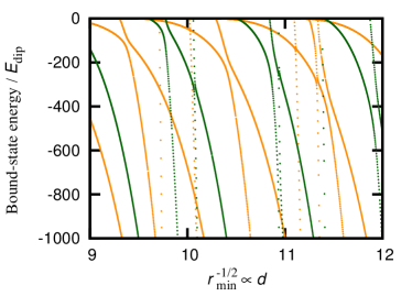
Figure 5: Bound states as a function of $r_{\mathrm{min}}^{-1/2}$, for odd $L$. Results shown in orange and green correspond to $M_{L}=0$ and $|M_{L}|=1$, respectively.

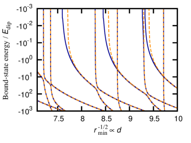
Figure 6: Bound states as a function of $r_{\mathrm{min}}^{-1/2}$, for even and odd $L$ and $M_{L}=0$ shown in blue and orange, respectively.

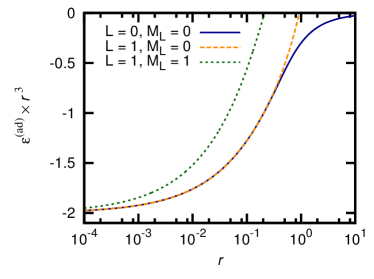
Figure 7: Adiabatic potential curves multiplied by $r^{3}$ for bosons ($L=0$) and fermions ($L=1$) for both $M_{L}=0$ and $1$.

V Lennard-Jones potential

In this section we employ a soft-wall boundary condition. We use a Lennard-Jones “short-range” potential in Eq. 1,

$$V_{\mathrm{SR}}(R)=C_{12}R^{-12}-C_{6}R^{-6}.$$ (11)

The $R^{-6}$ term is typically attractive and can model the dispersion or van der Waals interaction, whereas the $R^{-12}$ term describes short-range repulsion. In contrast with the dipole-dipole interaction, this short-range potential is completely isotropic. To adjust the short-range behavior, we vary the Lennard-Jones potential well depth,

$$D_{\rm e}=\frac{C_{6}^{2}}{4C_{12}},$$ (12)

while holding $C_{6}$ fixed. A length scale for the van der Waals interaction can be defined as

$$R_{6} =\left(\frac{2MC_{6}}{\hbar^{2}}\right)^{1/4},$$ (13)

with energy scale

$$E_{6}=\frac{\hbar^{2}}{2MR_{6}^{2}}.$$ (14)

For pairs of magnetic atoms, $R_{6}$ is comparable to the dipole length, whereas for pairs of polar molecules the dipole length is considerably larger.

Inclusion of the Lennard-Jones potential breaks the universality of the dipole-dipole interaction, as the bound states depend on the relative strength of the dispersion and dipole-dipole interactions. Below, we consider parameters that are typical for two cases: pairs of magnetic atoms, and pairs of polar molecules.

V.1 Magnetic atoms: $R_{\mathrm{dip}}\approx R_{6}$

Here we employ the parameters $C_{6}=2003\,E_{\rm h}a_{0}^{6}$ Maier et al. (2015), a magnetic dipole moment $\mu=9.93\mu_{\rm B}$, and reduced mass $M=81.96\,m_{\rm u}$, which correspond to bosonic ${}^{162}\mathrm{Dy}$. The Lennard-Jones well depth is varied around $D_{\rm e}\approx 800$ cm^-1 Petrov et al. (2012), such that it supports around 60 vibrational states for $L=0$. The length scales of the van der Waals, $R_{6}=154\leavevmode\nobreak\ a_{0}$, and dipole-dipole interaction, $R_{\mathrm{dip}}=196\leavevmode\nobreak\ a_{0}$, are roughly comparable. The Lennard-Jones potential nevertheless supports many more bound states than the dipole-dipole potential, because it is substantially deeper at short range.

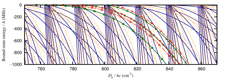
Figure 8: Bound states as a function of the Lennard-Jones well depth. States shown as solid blue lines have been obtained with parameters that are representative of magnetic atoms. Results shown as orange dashed lines are obtained with the dipole moment set to zero. Three states from each calculation are highlighted to guide the eye: in green (red) with the dipole on (off); squares are states on the lowest adiabat (asymptotically $L=0$), circles are states on the first excited adiabat ($L=2$), and triangles are states on the second excited adiabat ($L=4$).

Figure 8 displays bound states for even $L$ and $M_{L}=0$ as a function of the Lennard-Jones well depth, $D_{e}$. States shown in blue are from the full calculation, as described above, whereas those shown in orange were are for the pure Lennard-Jones potential without dipole-dipole interactions. The structure of the bound states of the full system closely resembles that of the pure Lennard-Jones potential, and the effect of the dipole-dipole interaction is essentially perturbative.

Figure 9 shows an expanded plot of the pure Lennard-Jones states with $L$ assignments, together with the $s$-wave scattering length. The structure of the near-threshold bound states of the pure Lennard-Jones potential is such that it groups together near-threshold states with $L=0,4,8,\ldots$, and the same holds for states with $L=2,6,10,\ldots$ Gao (2000, 2004). The bound states show periodicity as a function of the well depth, where bound states with $L=0,4,8,\ldots$ cross the dissociation threshold for well depths where the $s$-wave scattering length $a$ is infinite Gao (2000, 2004). Bound states with $L=2,6,10,\ldots$ cross threshold where $a$ is equal to the mean scattering length Gao (2000, 2004), $a=\bar{a}\approx 0.478R_{6}$ Gribakin and Flambaum (1993). Away from threshold, the bound states for different $L$ separate, varying more steeply with well depth for higher $L$.

This level structure leads to a grouping of states with $\Delta L\geq 4$, whereas the dipole-dipole coupling is non-zero only between states with $\Delta L=0,\pm 2$. This leads to a suppression of the effects of dipole-dipole coupling; crossings of Lennard-Jones states directly coupled by the dipole-dipole interaction do not occur near threshold . The main effect of dipole-dipole interaction is a shift of the bound-state energies, which is close to the first-order energy

$$E_{vLM_{L}}^{(1)}= -2d_{1}d_{2}\begin{pmatrix}L&2&L\\ 0&0&0\end{pmatrix}\begin{pmatrix}L&2&L\\ M_{L}&0&-M_{L}\end{pmatrix}$$

$$\times(-1)^{M_{L}}(2L+1)\langle vLM_{L}|R^{-3}|vLM_{L}\rangle.$$ (15)

The $L=0$ and $L=2$ states are notable exceptions. The $L=0$ states have no first-order shifts, whereas each $L=2$ state is shifted down in first order to near-degeneracy with the corresponding $L=0$ state. Higher-order couplings shift the $L=0$ states down considerably, and shift the $L=2$ states back up, coincidentally for this particular dipole moment to near the unperturbed Lennard-Jones level.

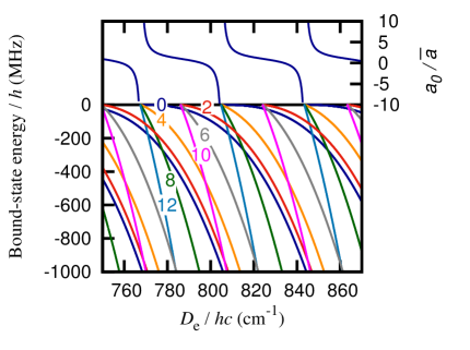
Figure 9: Bound states, including $L$ assignment, as a function of the Lennard-Jones well depth in the absence of dipole-dipole interactions. Also included is the $s$-wave scattering length, which sets the observed period.

V.2 Molecule-molecule: $R_{\mathrm{dip}}\gg R_{6}$

In this section, we perform calculations where the space-fixed dipole moment is scaled up by a factor of 10, which results in the equivalent of a space-fixed electric dipole moment of 0.92 Debye. This increases the dipole length $R_{\mathrm{dip}}$ by a factor 100, to 19600 $a_{0}\approx 1$ $\mu$m, and decreases the dipole energy $E_{\mathrm{dip}}$ by a factor of 10000, to 57 kHz $\times\ h$. In this case, the van der Waals potential provides a “short-range” boundary condition for the dipole-dipole coupling, which acts on a much larger length scale. The case $R_{\mathrm{dip}}\approx 100R_{6}$ is roughly typical for ultracold polar molecules, where the dispersion coefficient is dominated by the rotational contribution, $C_{6}=\mu^{4}/[(4\pi\epsilon_{0})^{2}\ 6B_{\mathrm{rot}}]$. Table 1 gives the molecule-fixed dipole moments $d^{\mathrm{lim}}$ and rotational $C_{6}$ coefficients for selected alkali-metal dimers. Also given are dispersion and dipole-dipole length scales, with the latter ($R_{\mathrm{dip}}^{\mathrm{lim}}$) calculated with the molecule-fixed dipole moment, and the electric field $F_{\mathrm{0.7}}$ at which the space-fixed dipole moment is approximately 0.7 times its molecule-fixed value and $R_{\mathrm{dip}}\approx R_{\mathrm{dip}}^{\mathrm{lim}}/2.$

Table 1: Molecular dipole moments and rotational $C_{6}$ coefficients for selected alkali dimers. Also included are the dipole and dispersion length scales, and their ratio. The dipole length is calculated for the limiting value of the space-fixed dipole moment. The applied electric field $F_{\mathrm{0.7}}$ needed to induce a dipole moment of $0.7$ times the limiting dipole moment – and to achieve approximately half the limiting dipolar length scale – is also included.

Molecule	$d^{\mathrm{lim}}$ (Debye)	$R_{\mathrm{dip}}^{\mathrm{lim}}$ / $a_{0}$	$E_{\mathrm{dip}}^{\mathrm{lim}}$ (Hz)	$C_{6}/E_{\rm h}a_{0}^{6}$	$R_{6}/a_{0}$	$E_{6}$ (kHz)	$R_{\mathrm{dip}}^{\mathrm{lim}}/R_{6}$	$F_{\mathrm{0.7}}$ (kV/cm)
KRb	0.57	$5.7\times 10^{3}$	1725	$2.4\times 10^{3}$	$154$	1200.6	37	22.2
RbCs	1.2	$4.7\times 10^{4}$	15.1	$1.2\times 10^{5}$	$469$	74.6	99	4.5
NaK	2.7	$6.6\times 10^{4}$	26.5	$5.1\times 10^{5}$	$491$	237.2	134	11.7
KCs	2.0	$9.5\times 10^{4}$	4.6	$4.5\times 10^{5}$	$613$	55.9	155	5.1
NaRb	3.3	$1.7\times 10^{5}$	2.3	$1.5\times 10^{6}$	$739$	60.0	229	7.1
CaF	3.1	$7.8\times 10^{5}$	19.9	$2.3\times 10^{5}$	$395$	391.3	198	37.7

Figure 10 shows the bound states as a function of the Lennard-Jones well depth. The density of states is approximately proportional to $E^{-2/3}$. The upper panel may be compared with the case of magnetic atoms in Fig. 8, where the density is lower and increases as about $E^{-1/2}$ because the attractive part of the Lennard-Jones potential dominates. The lower panel of Fig. 10 shows an expanded view of the molecule-molecule bound states, with the energy range reduced by a factor of $10^{4}$. In this range, there is a complicated level pattern with many avoided crossings, similar to that seen with a hard-wall boundary condition in Fig. 3. This contrasts with the case of magnetic atoms, shown in Fig. 8, where there are no significantly avoided crossings close to threshold. Although the periodicity with $D_{\mathrm{e}}$ is driven by the variation of the Lennard-Jones potential even in the molecular case, it is clear that the dipole-dipole interaction is no longer simply perturbative; instead, the Lennard-Jones effectively sets a short-range boundary condition for the dipole-dipole interaction, but the latter is now dominant and determines the structure of the states.

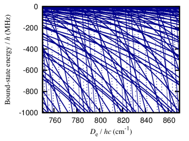
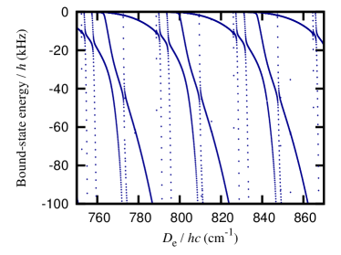
Figure 10: Dipole bound states with Lennard-Jones short-range interactions in the case $R_{\mathrm{dip}}\gg R_{6}$. Top: On the same scale as Fig. 8. Bottom: The vertical energy scale has been reduced by a factor $10^{4}$.

Figure 11 shows the states as a function of the space-fixed dipole moment with the Lennard-Jones well depth fixed. The structure observed is similar to that from the simpler calculations shown in Fig. 3, which used a hard-wall short-range boundary condition at a distance equal to the van der Waals length scale. However, the states in Fig. 11 have an approximate period of about 0.02 Debye, which is considerably shorter than in Fig. 3. This period corresponds to a hard wall around 7 $a_{0}$, which is comparable to the inner turning point of the Lennard-Jones potential. The lowest adiabat of the dipole-dipole interaction at $R_{6}=154\,a_{0}$ is about $-500E_{6}$, and at this kinetic energy the transmission coefficient through the attractive part of the Van der Waals potential is close to 1 Gao (2008).

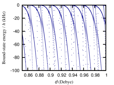
Figure 11: Dipole bound states with Lennard-Jones short-range interactions in the case $R_{\mathrm{dip}}\gg R_{6}$, as a function of dipole moment for a fixed well depth.

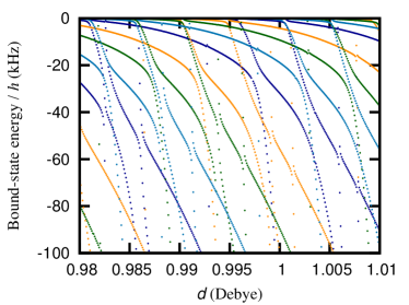
Figure 12: Dipole bound states with Lennard-Jones short-range interactions in the case $R_{\mathrm{dip}}\gg R_{6}$, as a function of dipole moment for fixed well depths. Different colors correspond to different well depths between roughly 800 and 830 cm^-1, which scans one cycle of scattering length.

Figure 12 shows the states over a smaller range of dipole moment for 4 different Lennard-Jones well depths over one period of the Lennard-Jones scattering length. Although each of these show different details in the states from higher adiabats, the overall dependence on the induced dipole moment is similar for each of the different well depths and also similar to that observed for hard-wall boundary conditions in Sec. IV. Since the pattern of states is independent of the short-range boundary conditions, it should be present for real systems and should be observable spectroscopically by measurements on trapped ultracold polar molecules.

VI Conclusions

We have explored the bound states of a simple model of the dipole-dipole interaction. The model assumes that both dipoles are oriented along a space-fixed field direction. It has been used extensively in the description of many-body physics with ultracold polar molecules and magnetic atoms, but its two-body physics has been explored less fully. We have studied the bound states of this model with both hard-wall boundary conditions and more realistic Lennard-Jones short-range interactions.

In the simplest case, with hard-wall boundary conditions, we find a complicated pattern of bound states that avoided-cross as a function of the boundary condition or the space-fixed dipole moment. The pattern of states may be understood using an adiabatic representation, which diagonalizes the dipole-dipole interaction at each separation of the dipoles. States supported by the lowest adiabatic potential curve approach threshold slowly as a function of dipole moment, while those supported by excited adiabats approach more steeply. The adiabatic approximation gives a good qualitative description of the energy levels, except near avoided crossings between levels supported by different adiabats.

The adiabats of a pure dipole-dipole potential are universal when expressed in terms of the dipole length and dipole energy defined in Eq. 4. For a pair of bosons, the lowest adiabat behaves as $-C_{4}R^{-4}$ at very long range. However, it deviates substantially from this form at distances around the dipole length. Because of this, the $R^{-4}$ form accurately describes states only if they are bound by much less than the dipole energy. The dipole energy decreases very fast as the dipole itself increases, and for pairs of polar molecules is typically less than 1 kHz $\times h$. This is so shallow that there are usually no states in the region characterized by the asymptotic $R^{-4}$ form.

For fermions, with odd $L$, states with $M_{L}=0$ are almost identical to the boson states when bound by more than the dipole energy. This may also be understood through the adiabatic representation, as the states can localize with dipoles head-to-tail in both cases. There are also fermion states with $|M_{L}|>0$, which are confined by a higher centrifugal barrier.

We have also considered two cases with a Lennard-Jones short-range potential in place of the hard-wall boundary condition. When the dipolar length scale is comparable to the van der Waals length scale, as is the case for magnetic atoms with weak dipolar interactions, the bound states are dominated by the Lennard-Jones potential, and the dipole-dipole interaction acts perturbatively. The dipole-dipole coupling is suppressed by the structure of van der Waals bound states, which groups together states with $\Delta L\geq 4$ that are not coupled directly by dipole-dipole interactions.

When the dipolar length scale is much larger than the van der Waals length scale, as is achievable for polar molecules with large dipole moments, there is a denser set of dipole-dipole bound states close to threshold. These states can be tuned across threshold by varying the dipole moment with an applied electric field and exhibit complex patterns of avoided crossings below threshold. Spectroscopic measurements of these bound states, and observation of resonances where they cross threshold, have great potential to help understand dipolar interactions and illuminate their role in few-body and many-body quantum systems.

References

- Micheli et al. (2006) A. Micheli, G. K. Brennen, and P. Zoller, Nature Phys. 2, 341 (2006).
- Baranov (2008) M. Baranov, Phys. Rep. 464, 71 (2008).
- Lahaye et al. (2009) T. Lahaye, C. Menotti, L. Santos, M. Lewenstein, and T. Pfau, Rep. Prog. Phys. 72, 126401 (2009).
- Baranov et al. (2012) M. A. Baranov, M. Dalmonte, G. Pupillo, and P. Zoller, Chem. Rev. 112, 5012 (2012).
- Astrakharchik et al. (2007) G. E. Astrakharchik, J. Boronat, I. L. Kurbakov, and Y. E. Lozovik, Phys. Rev. Lett. 98, 060405 (2007).
- Büchler et al. (2007) H. P. Büchler, E. Demler, M. Lukin, A. Micheli, N. Prokof’ev, G. Pupillo, and P. Zoller, Phys. Rev. Lett. 98, 060404 (2007).
- Cooper and Shlyapnikov (2009) N. R. Cooper and G. V. Shlyapnikov, Phys. Rev. Lett. 103, 155302 (2009).
- Capogrosso-Sansone et al. (2010) B. Capogrosso-Sansone, C. Trefzger, M. Lewenstein, P. Zoller, and G. Pupillo, Phys. Rev. Lett. 104, 125301 (2010).
- Macia et al. (2012) A. Macia, D. Hufnagl, F. Mazzanti, J. Boronat, and R. E. Zillich, Phys. Rev. Lett. 109, 235307 (2012).
- Barnett et al. (2006) R. Barnett, D. Petrov, M. Lukin, and E. Demler, Phys. Rev. Lett. 96, 190401 (2006).
- Gorshkov et al. (2011) A. V. Gorshkov, S. R. Manmana, G. Chen, E. Demler, M. D. Lukin, and A. M. Rey, Phys. Rev. A 84, 033619 (2011).
- Yan et al. (2013) B. Yan, S. A. Moses, B. Gadway, J. P. Covey, K. R. A. Hazzard, A. M. Rey, D. S. Jin, and J. Ye, Nature 501, 521 (2013).
- Zou et al. (2017) H. Zou, E. Zhao, and W. V. Liu, Phys. Rev. Lett. 119, 050401 (2017).
- Lahaye et al. (2008) T. Lahaye, J. Metz, B. Fröhlich, T. Koch, M. Meister, A. Griesmaier, T. Pfau, H. Saito, Y. Kawaguchi, and M. Ueda, Phys. Rev. Lett. 101, 080401 (2008).
- DeMille (2002) D. DeMille, Phys. Rev. Lett. 88, 067901 (2002).
- Lukin et al. (2001) M. D. Lukin, M. Fleischhauer, R. Cote, L. M. Duan, D. Jaksch, J. I. Cirac, and P. Zoller, Phys. Rev. Lett. 87, 037901 (2001).
- Yelin et al. (2006) S. F. Yelin, K. Kirby, and R. Côté, Phys. Rev. A 74, 050301 (2006).
- Santos et al. (2004) L. Santos, M. A. Baranov, J. I. Cirac, H.-U. Everts, H. Fehrmann, and M. Lewenstein, Phys. Rev. Lett. 93, 030601 (2004).
- Büchler et al. (2005) H. P. Büchler, M. Hermele, S. D. Huber, M. P. A. Fisher, and P. Zoller, Phys. Rev. Lett. 95, 040402 (2005).
- Jaksch and Zoller (2005) D. Jaksch and P. Zoller, Ann. Phys. 315, 52 (2005).
- Griesmaier et al. (2005) A. Griesmaier, J. Werner, S. Hensler, J. Stuhler, and T. Pfau, Phys. Rev. Lett. 94, 160401 (2005).
- Beaufils et al. (2008) Q. Beaufils, R. Chicireanu, T. Zanon, B. Laburthe-Tolra, E. Maréchal, L. Vernac, J.-C. Keller, and O. Gorceix, Phys. Rev. A 77, 061601 (2008).
- Lu et al. (2011) M. Lu, N. Q. Burdick, S. H. Youn, and B. L. Lev, Phys. Rev. Lett. 107, 190401 (2011).
- Pasquiou et al. (2012) B. Pasquiou, E. Maréchal, L. Vernac, O. Gorceix, and B. Laburthe-Tolra, Phys. Rev. Lett. 108, 045307 (2012).
- Aikawa et al. (2012) K. Aikawa, A. Frisch, M. Mark, S. Baier, A. Rietzler, R. Grimm, and F. Ferlaino, Phys. Rev. Lett. 108, 210401 (2012).
- Ni et al. (2008) K.-K. Ni, S. Ospelkaus, M. H. G. de Miranda, A. Pe’er, B. Neyenhuis, J. J. Zirbel, S. Kotochigova, P. S. Julienne, D. S. Jin, and J. Ye, Science 322, 231 (2008).
- Takekoshi et al. (2014) T. Takekoshi, L. Reichsöllner, A. Schindewolf, J. M. Hutson, C. R. Le Sueur, O. Dulieu, F. Ferlaino, R. Grimm, and H.-C. Nägerl, Phys. Rev. Lett. 113, 205301 (2014).
- Molony et al. (2014) P. K. Molony, P. D. Gregory, Z. Ji, B. Lu, M. P. Köppinger, C. R. Le Sueur, C. L. Blackley, J. M. Hutson, and S. L. Cornish, Phys. Rev. Lett. 113, 255301 (2014).
- Park et al. (2015) J. W. Park, S. A. Will, and M. W. Zwierlein, Phys. Rev. Lett. 114, 205302 (2015).
- Guo et al. (2016) M. Guo, B. Zhu, B. Lu, X. Ye, F. Wang, R. Vexiau, N. Bouloufa-Maafa, G. Quéméner, O. Dulieu, and D. Wang, Phys. Rev. Lett. 116, 205303 (2016).
- Truppe et al. (2017) S. Truppe, H. J. Williams, M. Hambach, L. Caldwell, N. J. Fitch, E. A. Hinds, B. E. Sauer, and M. R. Tarbutt, Nat. Phys. 13, 1173 (2017).
- Rvachov et al. (2017) T. M. Rvachov, H. Son, A. T. Sommer, S. Ebadi, J. J. Park, M. W. Zwierlein, W. Ketterle, and A. O. Jamison, Phys. Rev. Lett. 119, 143001 (2017).
- McCarron et al. (2018) D. J. McCarron, M. H. Steinecker, Y. Zhu, and D. DeMille, Phys. Rev. Lett. 121, 013202 (2018).
- Ticknor (2008) C. Ticknor, Phys. Rev. Lett. 100, 133202 (2008).
- Bohn et al. (2009) J. L. Bohn, M. Cavagnero, and C. Ticknor, New J. Phys. 11, 055039 (2009).
- Braaten and Hammer (2006) E. Braaten and H.-W. Hammer, Phys. Rep. 428, 259 (2006).
- Hutson (2011) J. M. Hutson, (2011), BOUND computer code.
- Brink and Satchler (1994) D. M. Brink and G. R. Satchler, Angular Momentum, 3rd ed. (Clarendon Press, Oxford, 1994).
- Manolopoulos (1986) D. E. Manolopoulos, J. Chem. Phys. 85, 6425 (1986).
- Alexander and Manolopoulos (1987) M. H. Alexander and D. E. Manolopoulos, J. Chem. Phys. 86, 2044 (1987).
- Hutson (1994) J. M. Hutson, Comput. Phys. Commun. 84, 1 (1994).
- Johnson (1978) B. R. Johnson, J. Chem. Phys. 69, 4678 (1978).
- Ticknor and Bohn (2005) C. Ticknor and J. L. Bohn, Phys. Rev. A 72, 032717 (2005).
- Maier et al. (2015) T. Maier, H. Kadau, M. Schmitt, M. Wenzel, I. Ferrier-Barbut, T. Pfau, A. Frisch, S. Baier, K. Aikawa, L. Chomaz, M. J. Mark, F. Ferlaino, C. Makrides, E. Tiesinga, A. Petrov, and S. Kotochigova, Phys. Rev. X 5, 041029 (2015).
- Petrov et al. (2012) A. Petrov, E. Tiesinga, and S. Kotochigova, Phys. Rev. Lett. 109, 103002 (2012).
- Gao (2000) B. Gao, Phys. Rev. A 62, 050702 (2000).
- Gao (2004) B. Gao, Eur. Phys. J. D 31, 283 (2004).
- Gribakin and Flambaum (1993) G. F. Gribakin and V. V. Flambaum, Phys. Rev. A 48, 546 (1993).
- Note (1) In the presence of an anisotropic dispersion interaction, channels with different values of may have different effective coefficients; this would lift the threshold degeneracy between states with and might result in crossings between states with that are coupled by the dipole-dipole interaction.
- Gao (2008) B. Gao, Phys. Rev. A 78, 012702 (2008).