Deep multi-task learning for a geographically-regularized semantic segmentation of aerial images

Abstract

This is the pre-acceptance version, to read the final version published in the ISPRS Journal of Photogrammetry and Remote Sensing, please go to: 10.1016/j.isprsjprs.2018.06.007.

When approaching the semantic segmentation of overhead imagery in the decimeter spatial resolution range, successful strategies usually combine powerful methods to learn the visual appearance of the semantic classes (e.g. convolutional neural networks) with strategies for spatial regularization (e.g. graphical models such as conditional random fields).

In this paper, we propose a method to learn evidence in the form of semantic class likelihoods, semantic boundaries across classes and shallow-to-deep visual features, each one modeled by a multi-task convolutional neural network architecture. We combine this bottom-up information with top-down spatial regularization encoded by a conditional random field model optimizing the label space across a hierarchy of segments with constraints related to structural, spatial and data-dependent pairwise relationships between regions.

Our results show that such strategy provide better regularization than a series of strong baselines reflecting state-of-the-art technologies. The proposed strategy offers a flexible and principled framework to include several sources of visual and structural information, while allowing for different degrees of spatial regularization accounting for priors about the expected output structures.

1 Introduction

This paper deals with parsing decimeter resolution abovehead images into semantic classes, relating to land cover and/or land use types. We will refer to this process as semantic segmentation. For a successful segmentation, one requires visual models able to disambiguate local appearance by understanding the spatial organization of semantic classes [14]. To this end, machine learning models need to exploit different levels of spatial continuity in the image space [6, 40]. Accurate land cover and land use mapping is an active research field, growing in parallel to developments in sensors and acquisition systems and to data processing algorithms. Applications ranging from environmental monitoring [2, 12] to urban studies [47, 21] benefit from advances in processing and interpretation of abovehead data.

Semantic segmentation of sub-decimeter aerial imagery is often tackled by Markov and conditional random fields (MRF, CRF) [4, 26] combining local visual cues (the unary potentials) and interaction between nearby spatial units (the pairwise potentials) [22, 18, 47, 40, 43]. By maximizing the posterior joint probability of a CRF over the labeling (i.e. minimizing a Gibbs energy), one retrieves the most probable labeling of a given scene, i.e. the most probable configuration of local label assignments over the whole image space. These frameworks allow to model jointly bottom-up evidence, encoded in the unary potentials, together with some domain specific prior information encoded in the spatial interaction pairwise terms.

The idea behind the proposed model is that, when dealing with urban imagery (and in general decimeter resolution imagery), both the content of the image and the classes are highly structured in the spatial domain, calling for data- and domain-specific regularization. To follow such intuition, we model two key aspects of spatial dependencies: input and output space interactions. The former are usually encoded by operators accounting for the spatial autocorrelation of pixels in their spatial domain. The latter are encoded by different kinds of pairwise potential, favoring specific configurations issued from a predefined prior distribution.

• To extract information about local input relations, we combine state-of-the-art convolutional neural networks (CNN, [28, 41, 25]) providing data-driven cues for multiple tasks: We employ a CNN to not only provide approximate class-likelihoods, but also to predict semantic boundaries between the different classes. The latter coincide usually with natural edges in the image, but also corresponding to changes in labeling. Then, we build a segmentation tree using the semantic boundaries predicted by the CNN. Such tree represents hierarchy of regions spanning from the lowest level defined by groups of pixels (or superpixels) to the highest level, the whole scene. The region partitioning depends jointly on shallow-to-deep visual features and the semantic boundaries learned by the multi-task CNN.

• To account for the output relations between regions, we combine the information within each region in a hierarchy using a top-down graphical model model including different key aspects of the spatial organization of labels, given the observed inputs. This second modeling step is based on a CRF that aims at reducing the complexity (i.e. regularizing) of the pixel-wise maps, by semantically and spatially parsing consistent regions of the image, likely to belong to given classes, at different scales. Specifically, the CRF model takes into account evidence from the CNN (class-likelihoods, learned visual features and presence of class-specific boundaries) and spatial interactions (label smoothness, label co-occurrence, region distances, elevation gradient) within the hierarchy. In other words, it learns the extent and the labeling of each segment simultaneously, by minimizing a specifically designed energy.

A visual summary of the proposed pipeline is presented in Figure 1.

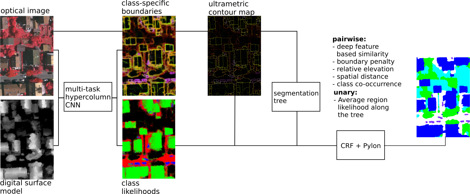
Figure 1: Flowchart of the proposed pipeline: from multi-modal inputs and multi-task learning to multi-modal and geographically regularized semantic segmentation.

We evaluate all the components of the system and show that spatial regularization is indeed useful in simplifying class structures spatially, while achieving accurate results. Since spatial structures are learned and encoded directly in the output map, we believe our pipeline is a step towards systems yet based on machine learning, but not requiring extensive manual post-processing (e.g. local class filtering, spatial corrections, map generalization, fusion and vectorization [8, 19]), at the same time employing domain knowledge and data specific regularization, tailoring it to specific application domain and softening black-box effects. Specifically, the contributions of this paper are:

• A detailed explanation on our multi-task CNN, building on top of a pretrained network (VGG);

• A strategy to transform semantic boundaries probabilities to superpixels and hierarchical regions;

• A CRF encoding the desired space-scale relationships between segments;

• The combination of different energy terms accounting for multiple input-output relationships, combining bottom-up (outputs and features of the CNN) and top-down (multi-modal clues about spatial arrangement) into local and pairwise relationships.

In the next Section, we summarize some relevant related works. In Section 3, we present the proposed system: the multi-task CNN architecture (Sec. 3.1), the hierarchical representation of image regions (Sec. 3.2) and the CRF model (Sec. 3.3). We present data and experimental setup in Section 4 and the results obtained in Section 5. We finally provide a discussion about our system in Section 6, leading to conclusions presented in Section 7.

2 Related works

2.1 Mid-level representations

To generate powerful visual models, traditional methods compute local appearance models mapping locals descriptors to labels, over a dense grid covering the image space. Then, the relationships between output variables are usually modeled by MRF and CRF. Standard approaches to local image descriptors involve the use of local color statistics, texture, bag-of-visual-words, local binary patterns, histogram of gradients and so on [22, 18, 47, 43, 40].

However, the use of fixed shape operators causes an inevitable loss of geometrical accuracy, in particular on objects borders. The most common solution to this problem is to employ a locally adaptive spatial support, to either summarize precomputed dense descriptors or to retrieve new ones. This strategy is usually implemented by the use of superpixels, which are defined to be small spatial units, uniform in appearance, while matching the natural edges in the image [10]. Moreover, superpixels significantly reduce the number of atomic units to be processed and consequently the computational time.

2.2 Deep representations

Convolutional neural networks (CNN), learn a parametric mapping from inputs to outputs, sidestepping the definition of i) an explicit processing resolution, ii) the type of appearance descriptors best representing the data, iii) a classifier to map descriptors to output labels [28, 41, 25]. The fact that a CNN learns an end-to-end mapping from data to outputs directly within the network makes deep neural networks more than valid alternatives to classical models, since complex feature engineering is avoided. However, most of these methods still rely on a fixed spatial support, either in the form of a patch to be classified (for patch classification) or in the form of the convolution kernel (for fully convolutional architectures) [31]. This can cause boundary blur and loss of definition on small image details. But despite blurring effects related to the size of the field of view, fully convolutional architectures are of particular interest for semantic segmentation. These techniques provide impressive accuracy and, once the architecture and hyperparameters are set, can be trained with ease as long as enough training data is available to learn the parameters.

For aerial and satellite image semantic segmentation, fully convolutional architectures are becoming state-of-the-art. A notable work in this direction is by Sherrah [39], where the author modifies a pretrained network to not downsample and performs dense semantic segmentation directly. In our previous work [44], we explored the use of deconvolutions to learn upsamplings providing outputs of the same resolution as inputs. Results outperformed standard patch-based strategies, both in terms of accuracy metrics and computational time, suggesting that fully convolutional architectures are best suited for semantic segmentation. In [34] we extended standard CNN to incorporate rotation invariance at the convolutional kernel level, resulting in small and compact models, but providing accuracy comparable to state-of-the-art architectures. Maggiori et al. [32] showed that a slightly modified hypercolumn architecture (originally proposed in [16]) is well suited for semantic segmentation of aerial images. Hypercolumns architectures exploit the entirety of the multiscale structures learned within the network, by upsampling intermediate activations and stacking them into a hypercolumn layer. On top of the latter, another sub-network learns to map to desired outputs, by exploiting the stack of multiscale structures, that can be seen as input features to this sub-network, and learning how to combine them. This is desirable for a model working in a highly structured input-output space with unique and explicit spatial relations. Due to these properties, we also adopt a modification of the hypercolumn architecture, which we detail in Section 3.1.

2.3 Learning boundary detectors

In this work we propose a multi-task CNN architecture to jointly learn a semantic segmentation task and a semantic boundary detection task. This latter task relates to supervised learning of semantic boundaries, as introduced in [15]. Authors proposed to combine bottom up edge detectors with object detectors in the image to enhance boundaries semantically The framework presented in the latter work has been reformulated in terms of deep learning [38, 45, 23, 33].

Usually, the prediction of boundaries supports semantic segmentation tasks, as the edges are naturally embedding shape information and contours of semantic classes. Such ideas have been exploited in computer vision since years (see e.g. the works stemming from [1]) and now also framed as deep learning systems [24, 33] or [35] for an example in aerial image segmentation.

In this work we build on the idea to retrieve semantic boundaries for one specific semantic class at a time. In this respect, we implement a sort of situational boundary detector [42], but rather than training a boundary detector on groups of images with similar appearance we train it on binary subproblems. More specifically, we train our detector to learn boundaries of one class at a time, versus non-edges for that class. For instance, we would learn a building versus non-building boundary detector, resulting in only building contours to be learned.

2.4 Models of output structures

Most CRF formulations model the conditional smoothness of the labels in the output space [5], facilitating two neighboring locations to share the same label if the mutual local appearance is similar. It is also common to incorporate information about the prior distribution of the label by weighting this potential with information about the statistical co-occurrence or relative location of labels at neighboring locations [14].

In Volpi and Ferrari [43] the energy employed to perform semantic segmentation is composed by a contrast-sensitive spatial quantization of label interactions allowing to learn specific dependencies at different scales with a structured Support Vector Machine. Hoberg et al. [18] present an approach not only modeling spatial dependencies at different scales, but also including class-specific temporal transition probabilities. Hedhli et al. [17] propose a hierarchical CRF to model image time series of different spatial resolution, where the hierarchy copes with the different scales represented in the image. Zheng et al. [46] propose a semantic segmentation system exploiting a hierarchy of labels in order to flexibly deal with possibly different labelings of the image. The auxiliary labels for each region in the images are modeled by a CRF. Golipour et al. [13] exploit a hierarchy of regions built by region-merging into a MRF model. They also extrapolate a score over edges of regions by checking relationships in the hierarchy. Finally, Li et al. [30] rely on a higher-order CRF to jointly infer at pixel and region level whether pixels and regions belong to rooftops or not. The line followed by these works show that accounting for hierarchical relationships jointly with the spatial distribution of labels allows for more expressive models.

In this paper we model spatial dependencies by following this last line of works. We employ a segmentation tree to encode multilevel likelihoods, in which regions merged according to learned and input cues should approximate object extent, and thus favoring a geometrically and semantically accurate segmentation.

3 Deep parsing of aerial images

Our model is composed of three main ingredients: a multi-task CNN providing class-likelihoods and probabilities of boundaries (Section 3.1), a segmentation tree (Section 3.2) and a CRF model encoding information about spatial dependency of the labeling (Sect. 3.3).

3.1 Multi-task CNN

Figure 2(a) presents the general network architecture. It closely follows the hypercolumn architectures presented in [16] (illustrated in Figure 2(b)), then used in [32] (Figure 2(c)), yet with small differences from both.

The main trunk of the network consists in a standard classification network, specifically the VGG-16 network pretrained on the ImageNet Image Large Scale Visual Recognition Challenge (ILSVRC) [41], which maps fixed size inputs to class scores. However, differently from other works employing pretrained networks, we remove the last fully connected layers and the last convolutional block and add two additional task-specific sub-networks to learn semantic segmentation and semantic boundary detection jointly. We do so, after rearranging the whole structure to follow the hypercolumns strategy [16].

Deep neural networks learn mappings with increasing abstraction power: from inputs to deep layers the learned features span from general and basic image descriptors (e.g. gradient detectors) to semantic concepts. The hypercolumn strategy aims at making use of such hierarchical abstraction in a more general framework, supporting fully convolutional architectures, and therefore no longer dependent on the extent of spatial activations.

To this end, such architectures resample activations from each block and we learn a mapping to the hypercolumn layer. On top of this hypercolumn, one or more convolutional layers learn a mapping into class scores. The rationale behind is that, by combining different levels of information, the first fully connected layer is not exclusively dependent from the activations learned sequentially up to that point, but can reuse previous activations if the problem requires so. This idea has been further extended in the DenseNet architectures [20].

Differently from standard hypercolumn models, we jointly learn two tasks on top of the hypercolumn stack: a semantic segmentation and a semantic boundary task. To this end, the network learns jointly two independent branches composed by two layers and a class score layer each (one per task). The semantic segmentation and the semantic boundary tasks are learned by minimizing a standard weighted cross-entropy loss, but with different scores aggregation strategies. This choice follows logically from the fact that a given pixel can belong to several semantic boundaries at the same time, typically two or three, while usually can only belong to a single semantic class.

The global loss function is given by a linear combination of the independent losses for each task $t$ as:

$$\mathcal{L}(y,\hat{y})=\sum_{i\in\{S,B\}}\beta_{t}\mathcal{L}^{i}(y,\hat{y}),$$ (1)

where $\beta$ balances the contribution of each loss. We observed that changing this hyperparameter modifies the speed of convergence of a task at the expense of the other. Loss scaling does not seem to be a problem as each multi-task branch is independently learned. Therefore, we set the contribution of both losses to be equal.

Both functions are defined by cross-entropy losses: the semantic segmentation loss $\mathcal{L}^{S}$ as:

$$\mathcal{L}^{S}(y,\hat{y})=-\frac{1}{N}\sum_{c}\omega_{c}\llbracket y_{i}=c\rrbracket\ \log\big{(}p(y_{i}=c|x_{i})\big{)},$$ (2)

where $N$ is the number of pixels in every input patch, $y_{i}$ is the ground truth class assigned to pixel $i$ and $\hat{y}_{i}$ the prediction. The posterior $p(y_{i}=c|x_{i})$ is obtained by normalizing the activations through a sigmoid. The cross-entropy loss puts all the mass on a single class $c$, meaning that an increase in the posterior probability for one class corresponds to a decrease in another one.

Regarding learning the semantic boundaries, we define the loss $\mathcal{L}^{B}$ as the average cross-entropy loss computed for each semantic boundary subproblem, as:

$$\mathcal{L}^{B}(y_{i},\hat{y}_{i}) =\sum_{b}\mathcal{L}^{b}(y^{b}_{i},\hat{y}^{b}_{i})$$

$$=-\frac{1}{N}\sum_{b}\omega_{b}\llbracket y^{b}_{i}=b\rrbracket\ \log\big{(}p(y^{b}_{i}=b|x_{i})\big{)},$$ (3)

where $y^{b}_{i}$ and $\hat{y}^{b}_{i}$ are the binary ground truth and prediction for the $b$th binary semantic boundary problem for pixel $i$. The posteriors $p(y^{b}_{i}=c|x_{i})$ are again obtained by normalizing the activations through a sigmoid.

Therefore, the final loss allows a given pixel to be predicted as boundary across several classes. Recall that, since we approach modeling semantic boundaries as separate sub-problems, every $b$th task involves modeling only the semantic boundaries of class $b$, pooling non-boundary pixels and boundaries from other classes.

Both losses are weighed for each class by $\omega$: for the segmentation loss, we set a weight proportional to the inverse class frequency [36], while for boundary we weigh errors on boundaries by 0.99, while on non-boundaries 0.01, since the prior probability of boundary pixels is extremely low [45].

During backpropagation, only the partial derivative of the total loss of Eq. (2) with respect to the weight for one task is non-zero. Therefore, only the sub-loss computed at one output backpropagates gradients for a specific task. Gradients at the hypercolumn layer are added and backpropagated through the intermediate layers and added again to those coming from the layers of the main trunk. Learning rates are scaled by a factor $10^{-3}$ on the layers pretrained on the ILSVRC ImageNet.

Differently from [16], we do not sum activations at the hypercolumn layer, since in their model each intermediate layer is a classifier. Although this is a very effective way for single tasks, in our model we needed more flexibility to learn both tasks jointly. To this end, we stacked the input image to activations derived from the rectified linear units nonlinearities (ReLU) of the classification network. This composes the input to both fully connected layers, composed by two layers. On the other hand, our model does not simply stack resampled activations, but also learns an intermediate mapping from the ReLU to the hypercolumns by a convolutional block (see Figure 2). We observe this strategy to be beneficial for three main reasons: first, it allows the hypercolumn layer to be composed by slightly altered activations, closer to the tasks that we want to learn. This is especially important when using pretrained networks, since, although being related, tasks and modality of our problem differ to those of the ImageNet ILSVRC. Secondly, we map arbitrarily sized mid-representations from ReLUs to activations of same dimensionality, typically smaller or equal to the dimensionality of the original ReLU activations. Although this might seem unimportant since we stack activations (contrarily to [16] where the hypercolumn is a sum of activations), it still has at least three main benefits:

• It allows to control the dimensionality of the hypercolumn stack and the total number of learnable parameters

• We distill information closely related to the tasks at hand by keeping the added layers lower-dimensional

• Intermediate features also learn important local correlations in the feature maps, since these intermediate mappings are learned by standard convolutional layers.

When coupled to the effective field of view of the classification network and to the spatial resampling needed to stack activations into the hypercolumns, the fully connected layers have at their disposal information about features carrying different levels of abstraction and accounting for different degrees of spatial dependencies, both short- and long-range. Note that at this level we also include the original optical image and information about the elevation (in the form of a normalized digital surface model), so effectively coupling the power of large scale pretrained network to extract features and additional information which could not be fed to it.

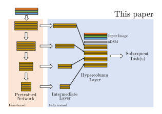
(a)
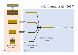
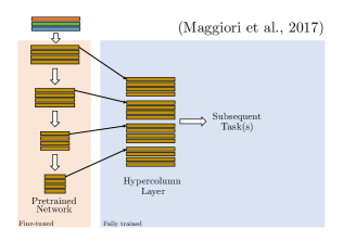
(b)	(c)

Figure 2: A comparison of three hypercolumn architectures. In all images, white empty arrow means learned convolutions while thin arrows correspond to bilinear upsampling. (a) shows our architecture, (b) the one from [32] and (c) the original hypercolumn as presented by [16]. Note that this last one, since sums responses from activation-specific classifiers, cannot be used for multitask learning out of the box.

3.2 From probability of semantic boundaries to segmentation trees

In the presented pipeline, we use the learned semantic boundaries at two different levels in our pipeline: as a pairwise potential in the CRF model (see Eq. (7)) and as features to retrieve the segmentation tree, whose delineation is explained in this section.

In order to obtain a segmentation tree common to all classes, we combine the semantic boundary probabilities into a score $g$. This score denotes the maximum posterior probability for a pixel $\mathbf{x}_{i}$ to belong to a semantic boundary in task $\mathcal{L}^{B}$ (Eq. (3)):

$$g(\mathbf{x}_{i})=\max_{b}\left(p(y^{b}_{i}|\mathbf{x}_{i})\right).$$

This ensures that, independently of the semantic boundary class, strong edges always prevail over weak ones, enabling us to obtain the most probable segmentation tree. We will employ the learned class-specific boundaries in the CRF model.

Before building the segmentation tree, we transform the boundary scores $g(\mathbf{x})$ into an ultrametric contour map (UCM, Arbelaez et al. [1]). An UCM defines a hierarchy of non-overlapping and closed contours based on a boundary probability score. The basic level of the hierarchy is defined by region contoured by low-probability boundaries, which in our case is defined by a watershed oversegmentation, where the landscape is defined by $g(\mathbf{x})$. Moving up in the segmentation tree, only boundaries with stronger UCM contours define closed contours. The attractive property of UCMs is that, for a given edge between two regions, the score is constant and defines a natural dissimilarity metric across regions.

In order to build the segmentation tree, we complement the UCM dissimilarity with other two metrics defined over regions: the Euclidean distance between per-region average hypercolumn activation $\mathbf{x}^{h}$ and the Euclidean distance between region centroids $\mathbf{x}^{c}$ in the spatial domain. The former provides high-level information about region contents, while the second favors small isolated regions to be clustered to a nearby neighbor. For any two regions $i,j$, these distances are defined as $\mathbf{D}_{ij}=\|\mathbf{x}_{i}-\mathbf{x}_{j}\|_{2}$ by employing the appropriate feature vector in $\mathbf{x}$. If we define these three dissimilarities as $\mathbf{D}^{g}$, $\mathbf{D}^{h}$, $\mathbf{D}^{c}$ for the UCM, hypercolumn and spatial distance, respectively, our final segmentation tree is defined by clustering regions based on a convex combination ($\sum_{i}w_{i}=1$): $\mathbf{D}^{*}=w_{1}\mathbf{D}^{g}+w_{2}\mathbf{D}^{h}+w_{3}\mathbf{D}^{c}$. The type of distances reflect those used as pairwise potentials. Their normalization and the weights $w$ are selected based on the average class purity per leaf region on validation images. We observed that the UCM dissimilarity tends to receive the highest weight, followed by the hypercolumn distances and spatial distance. Note that we will also use these dissimilarities in the CRF model described below.

3.3 Semantic segmentation model

Our CRF model is defined over the regions of the segmentation tree, and not over pixels directly. The main assumption behind this choice is that every pixel is covered by a set of regions with different sizes and somewhere, along the tree, the region which best explains the semantic land-cover classes is present. Given this assumption, we naturally chose to employ the Pylon model [29]. The Pylon model is an inference framework that, given a segmentation tree and relationships across leaf regions, finds the most probable tree cut and segmentation. This is done by exploiting pairwise spatial smoothness terms and local evidence about class likelihoods together. Such joint optimization allows flexibility to choose whether large segments are better than superpixels to describe a given region or if smaller ones are to be preferred in order to respect objects boundaries.

We model the joint probability of a labeling given the data as a Gibbs distribution $p(y|\mathbf{x})\approx\exp\left(-E(y;\mathbf{x})\right)$. To obtain the most probable label assignment (maximum-a-posteriori inference), one has to find among all possible label permutations for every possible semantic segmentation map, the one minimizing energy $E(y;\mathbf{x})$.

We define the energy over the pairwise graph $\mathcal{G}=(\mathcal{V},\mathcal{E})$, where every $i\in\mathcal{V}$ denotes a node (i.e. a region) with neighbors $j\in\mathcal{E}_{i}$. Specifically, we define the CRF as:

$$E(y;\mathbf{x})=\sum_{i\in\mathcal{V}}\Big{(}\varphi(y_{i};\mathbf{x}_{i})+\sum_{j\in\mathcal{E}_{i}}\mu(y_{i},y_{j})\phi(y_{i},y_{j};\mathbf{x}_{i},\mathbf{x}_{j})\Big{)}.$$ (4)

In the above model $\varphi(y_{i};\mathbf{x}_{i})$ is the cost of including in the labeling region $i$ with label $y$, given some evidence $\mathbf{x}$, while the term $\phi(y_{i},y_{j};\mathbf{x}_{i},\mathbf{x}_{j})$ is a combination of four different pairwise potentials and it takes into account the interactions between different labelings of two neighboring regions $i,j$. The pairwise function $\mu(y_{i},y_{j})$ provides a term accounting for global compatibility of labels. The rest of this section details all these terms.

Unary - $\varphi(y_{i},\mathbf{x}_{i})$

The unary potential is the negative log-likelihood provided by the CNN using task $\mathcal{L}^{S}$v (Eq. (2)) for each region in the segmentation tree. First, the dense per-pixel prediction of the CNN is averaged over leaf regions, for each class. This provides a rough approximation of the class-likelihood for each region, given their appearance modeled by the CNN. However, since we are dealing with a segmentation tree, the larger the region the more entropic the average probability, due to larger noise and variability. Therefore, to allow to select also parent regions, we weigh each unary by the size (in pixel) of its region, after transformation to standard scores. We define the unary potential as:

$$\ varphi(y_{i};\mathbf{x}_{i})=-\log\left(a_{i}^{\gamma}p(y_{i}|\mathbf{x}_{i})\right),$$ (5)

where $a_{i}$ denotes the area of region $i$ and $\gamma$ is a parameter controlling the spread of the values.

Interaction terms - $\phi(y_{i},y_{j};\mathbf{x}_{i},\mathbf{x}_{j})$

The interaction terms account for a series of prior beliefs about the spatial organization of classes and their interactions. In this work, this term is a sum of the four terms below, weighted by $\boldsymbol{\lambda}$:

1. Label smoothness. This potential encourages neighboring nodes to share the same label if the visual appearance of the regions is similar. It is usually based on a similarity across edges, so that connected nodes having similar colors but different labels penalize the energy more than two regions having different color, and therefore a low similarity.

   In our formulation we do not only use the input color similarity, but also deep features learned specifically for the problem. To this end, we average the activations stacked in the hypercolumn layer for each region. Remind that the hypercolumn layer contains information ranging from the input image to higher level visual concepts. If we denote $\mathbf{x}^{h}$ as the set of average features from the hypercolumn layer, the label smoothness pairwise energy is defined as:

   $$\phi^{h}(y_{i},y_{j};\mathbf{x}^{h}_{i},\mathbf{x}^{h}_{j})=\exp\left(\frac{-\|\mathbf{x}^{h}_{i}-\mathbf{x}^{h}\|^{2}_{2}}{\sigma^{h}}\right).$$ (6)

   The hyperparameter $\sigma^{h}$ is set as the median squared Euclidean distance between features of all the connected regions.

2. Edge Penalty. The edge penalty favors neighbors to share a similar label if no strong semantic edge separates the regions. This potential relies on the notion that two given adjacent regions can be very different in color, but belonging to the same semantic class. The information brought by learned boundaries aims at compensating such situations, by bringing new bottom-up evidence about label smoothness, this time accounting for local geometric features. We define this potential as:

   $$\phi^{g}(y_{i},y_{j};\mathbf{x}^{g}_{i},\mathbf{x}^{g}_{j})=\exp\left(\frac{-\theta(\mathbf{x}^{g}_{i},\mathbf{x}^{g}_{j})}{\sigma^{g}}\right),$$ (7)

   where $\theta(\mathbf{x}^{g}_{i},\mathbf{x}^{g}_{j})$ is the UCM score on the separating edge across two neighboring regions. As for the label smoothness potential, $\sigma^{g}$ is set as the median UCM score across neighbors.

3. Spatial distance. This potential considers spatial distances between region centroids. Leaf regions can be of different size. Usually, small regions whose centroids are close to each other tend to belong to the same class, while large regions with far apart centroids tend to belong to different classes. This potential scales the energy with respect to the spatial distance across regions, forcing smoothing to be stronger for close-by regions and softer for regions with far apart centroids. Its effect is to avoid having small isolated regions, independently on color or edge strength. This potential is defined as:

   $$\phi^{c}(y_{i},y_{j};\mathbf{x}^{c}_{i},\mathbf{x}^{c}_{j})=\exp\left(\frac{-\|\mathbf{x}^{c}_{i}-\mathbf{x}^{c}_{i}\|^{2}_{2}}{\sigma^{c}}\right),$$ (8)

4. Elevation difference. This potential relies on the assumption that regions belonging to the same object will share similar elevation range:

   $$\phi^{e}(y_{i},y_{j};\mathbf{x}^{e}_{i},\mathbf{x}^{e}_{j})=\exp\left(\frac{-|\mathbf{x}^{e}_{i}-\mathbf{x}^{e}_{i}|_{1}}{\sigma^{c}}\right),$$ (9)

   where $\sigma^{e}$ is the median of the absolute difference (denoted as the $|\cdot|$ in the numerator). This potential is actually independent from the actual absolute elevation $\mathbf{x}^{e}$, since only relative local differences are considered. Also, note that the label smoothness potential already contains elevation information, where global region similarity is evaluated by considering the whole hypercolumn stack. Nevertheless, we opted for making such information more explicit by adding a dedicated, independently weighted potential.

Summing up all of the above, the final total pairwise potential $\phi(y_{i},y_{j};\mathbf{x}_{i},\mathbf{x}_{j})$ is given by the weighted sum of each independent potential, as:

$$\phi(y_{i},y_{j};\mathbf{x}_{i},\mathbf{x}_{j})=\lambda_{h}\phi^{h}(y_{i},y_{j};\mathbf{x}^{h}_{i},\mathbf{x}^{h}_{j})+\lambda_{g}\phi^{g}(y_{i},y_{j};\mathbf{x}^{g}_{i},\mathbf{x}^{g}_{j})\\ +\lambda_{c}\phi^{c}(y_{i},y_{j};\mathbf{x}^{c}_{i},\mathbf{x}^{c}_{j})+\lambda_{e}\phi^{e}(y_{i},y_{j};\mathbf{x}^{e}_{i},\mathbf{x}^{e}_{j})$$ (10)

Global label compatibility - $\mu(y_{i},y_{j})$

To complete Eq. (4), and to employ a more informative model that the standard Potts, we weigh the sum of the pairwise potentials of Eq. (10) by a co-occurrence score, biasing labels association depending on the pairwise co-occurrence probability observed in training data. This statistic carries important information about the spatial organization of classes and conveys semantic ordering into the model. For instance, it is very likely to have cars and streets spatially co-occurring, while it is improbable to have many cars being direct neighbors of water regions.

We estimate this statistic by decomposing the ground truth of the training images into superpixels (corresponding to the lowest level of the segmentation tree) and simply counting co-occurrences of labels for adjacent regions. As superpixels, we use the leaves in the segmentation tree described in Section 3.2.

Although estimating such statistic on segmented training images, overfitting is not an issue, as we only retrieve counts to parametrize a metric with a number of parameters equal to $C^{2}-C$, for $C$ classes. We do not employ directly the joint probability $p(y_{i},y_{j})$ but we count conditionally and then average to obtain a symmetric measure $p(y_{i}|y_{j})$. Our final label compatibility is given by the negative log-likelihood of this frequency:

$$\mu(y_{i},y_{j})=-\log\left(\frac{1}{2}\left(p(y_{j}|y_{i})+p(y_{i}|y_{j})\right)\right).$$ (11)

An example matrix for one of the dataset used in the experiments (Zeebrugges) is illustrated in Figure 3. Note that we force a null diagonal to enforce label smoothness.

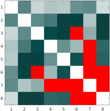
Figure 3: Example of compatibility label matrix between the classes of the Zeebrugges dataset (the class IDs are given in Section 4.2). Red cells denote co-occurrence of classes never observed in training, such as class pairs 7 (“Boats”) and 4 (“low vegetation”), 5 (“buildings”), 6 (“trees”) and 8 (“cars”). On the contrary, lighter colors denote more likely combinations, such as 1 (“impervious surfaces”) and 8 (“cars”).

3.4 Inference in the Pylon model

The Pylon model has been developed to perform semantic segmentation by jointly inferring regions extent and labels issued from a tree representation. The model imposes two main constraints on the segmentation: first, a single non-zero label must be assigned to every pixel, what Lempitsky et al. [29] call the completeness constraint. It implies that only one labeled region from the tree can cover the pixel, while the other regions defined over a specific location take the zero-label, i.e. inactive regions. This second requirement is made explicit by the non-overlap constraint, encoding the fact that overlapping regions cannot take non-zero labels. Both constraints are trivially met for a flat CRF, but become crucial constraints when making inference over a hierarchy of overlapping segments. We refer the interested reader to [29] for details about the reformulation of a CRF into a Pylon model.

One of the most interesting aspects of the pylon model is that inference can be performed by graph-cuts, thus taking advantage of the global optimality for the two classes case and of the efficiency. In our setting, we employ $\alpha$-expansion to perform inference with multiple classes. The Pylon models reformulates inference as a linear program leading to a pseudo-boolean optimization, which can be solved by the quadratic pseudo-boolean optimization (QPBO) [37].

4 Data and experimental setup

4.1 Vaihingen benchmark

The Vaihingen dataset is a dataset provided by the International Society for Photogrammetry and Remote Sensing (ISPRS), working group II/4, in the framework of a “2D semantic labeling contest” benchmark. .

The dataset is composed of 33 orthorectified image tiles acquired by a near infrared (NIR) - green (G) - red (R) aerial camera, over the town of Vaihingen (Germany). Images are accompanied by a digital surface model (DSM) representing absolute height of pixels. Gerke [11] released a normalized DSM, which represents the pixels height relative to the elevation of the nearest ground surface. We use this normalized DSM (nDSM) as an additional input to the hypercolumn layer.

The average size of the tiles is $2^{\prime}494\times 2^{\prime}064$ pixels with a spatial resolution of 9 cm. 16 out of the 33 tiles are fully annotated at pixel level and openly distributed to participants. In our experiments, we use 11 out of the 16 fully annotated image tiles for training (and hyperparameter selection), while the remaining ones (tile ID 11, 15, 28, 30, 34) for validation, as in Sherrah [39], Volpi and Tuia [44], Maggiori et al. [32]. The ground truths maps for the remaining tiles are undisclosed and used to evaluate the accuracy of submissions on an evaluation server run by the organizers.

The semantic segmentation task involves the discrimination of 6 land-cover / land-use classification classes: “impervious surfaces” (IS) (roads, concrete surfaces), “buildings” (BU), “low vegetation” (LV), “trees” (TR), “cars” (CA) and a class of “clutter” (CL) representing uncategorizable land covers. For this problem, classes are highly imbalanced: classes “buildings” and “impervious surfaces” cover 50% of the data, while “car” and “clutter”only for 2% of the total labels. Note that in our experiments, following the evaluation practice, we do not predict the class “clutter”. For the color coding of this dataset, we refer to Table 1.

4.2 Zeebrugges benchmark

This benchmark has been provided as part of the IEEE GRSS Data Fusion Contest in 2015 [7] .

This dataset is composed of seven tiles of size $10^{\prime}000\times 10^{\prime}000$ pixels. Single images have a spatial-resolution of 5 cm, which we downgrade to 10 cm for computational efficiency (in our past research [34] such downgrade did not lead to losses in performances after final upsampling of the predictions for evaluation). The images span RGB channels only. Five of the seven images are released with labels [27] and used for training and hyperparamter selection, while the remaining two are undisclosed for evaluating the generalization accuracy on an evaluation server, according to the challenge guidelines. Intuitively, the absence of a near infrared channel makes this dataset very challenging, even after resampling. The Zeebrugges dataset also comes with a LIDAR point cloud, that we transformed into a DSM by gridding and averaging the point cloud. As the area is relatively flat, there is no apparent need to normalize the DSM to relative heights. We include the DSM, together with the RGB images, at the hypercolumn layer.

This problem involves 8 classes [7]: the same six as in the Vaihingen benchmark, plus a land-cover “water” (WA) and a semantic class “boats” (BO). The class “clutter” (CL) represents a group of visual concepts semantically more uniform than in the Vaihingen benchmark. This class groups now mostly containers and other man made structures found in the harbor area. The classes distribution is also very unbalanced: the “water” class (in Vaihingen it was part of the “clutter” class) composes almost 30% of the annotated data, while while “cars” and “boats” labels account for 1% of the total. The color coding is presented in 3.

4.3 Experimental Setup

CNN architecture

We first train the architecture presented in Section 3.1. To this end, we employ the standard VGG-16 network [41], from which we remove the last (5th) convolutional block and the fully connected layers. Although the last layers could bring additional information, we argue that they are too specialized on the ImageNet ILSVRC classes. The multi-task layers learned on the hypercolumn stack have a similar purpose, which is to learn a high-level, task specific, convolutional layers. To train the network, we scale the learning rate of the pretrained VGG network to be 0.001 of the global learning rate and we increase the weight decay by a factor 10. We set the learning rate to $10^{-2}$ for Vaihingen and $10^{-3}$ for Zeebrugges. For Vaihingen, we half its value every 100 epochs for a total of 300 epochs. The weight decay has been set to 0.01 for 50 epochs to avoid initial spiking and then to 0.0005 for the rest. Inputs are $256\times 256$ patches with a minibatch size of 16. For Zeebrugges, we halve the learning rate after 200 epochs and train for another 200 epochs, with a constant weight decay of 0.0001. For Zeebrugges inputs are $500\times 500$ sub-tiles, and the minibatch set to 4. For both cases, the loss is weighted by a inverse frequency strategy, truncated when the inverse frequency is larger than 10. Note that a small random subset of the training patches is used for model selection, on which architectural choices and hyperparameters are selected. for both dataset, 10% of the training patches are randomly held out at each run and used as a development set.

For the Vaihingen experiments, we learn 20-dimensional $3\times 3$ nonlinear mappings from each VGG layer to the hypercolumn, with the exception of the last layer which is only a $1\times 1$, thus being a fully connected layer. For the Zeebrugges experiments, the architecture is the same but we employ 15-dimensional transitional layers. We fixed the kernel sizes to 3x3 and we selected the dimensionality of the activation based on the error on a small random held-out subset of the training set patches, after 50 epoch. Every activation is upsampled at the original input size by using bilinear interpolation, after learning the layer specific convolutional mapping. We did not experiment with learned upsampling and other complex interpolation strategies. This line of works could be an interesting extension in the future. We add two parallel $3\times 3$ layers, mapping from the hypercolumn stack to a 25-dimensional activation space, followed by a fully connected layer for each branch with the same dimensionality. One branch densely maps to semantic classes, while the other scores densely the semantic boundaries.

Semantic boundary ground truths

Our system is based on a two-tasks hypercolumn network, optimizing one loss on the semantic segmentation task (Eq. (2)) and a second one on the semantic boundaries extraction task (Eq. (3)). If the ground truth for the semantic segmentation task is a classical ground truth as the one provided in the two datasets used in this work (for an example in the Vaihingen dataset, see Figure 5(b)), building a ground truth to learn the semantic boundaries is less straightforward: to do so, we extracted all the binary semantic boundaries from the ground truth (e.g. between buildings and the rest, between cars and the rest) and used them as boundary classes (see Figure 7 for an example of predictions reflecting this scheme). It is built so that only 1 pixel thick line of pixels at the internal part of the object are considered as edges, which means that two ground truth edges never overlap and always lie one next to each other. Globally, for the employed datasets, this means 5 GT for the Vaihingen and 8 GT for the Zeebrugges datasets.

Inputs

As the input to VGG has to be three-dimensional, we input the nDSM only at the hypercolumn layer. We believe this strategy is more natural: first, as the VGG network is specialized in extracting visual concepts from natural images, we let the pretrained network to work only on the optical domain, by allowing some adjustment brought by fine tuning. This avoids an unnatural stack of elevation and visual information directly at the input layer, or even more artificial 3-dimensional inputs such as grayscale stacks. Although many works underline that non-standard input spaces still perform well, e.g. [35, 39], we prefer to use nDSM as a feature and not as a visual input. Secondly, by following the hypercolumn philosophy, VGG can be seen as a feature extractor and only after we learn a “second” convolutional neural network performing segmentation. Summing up, at the hypercolumn layer we concatenate i) elevation information, ii) the original input image and iii) the activations learned from the VGG. Studying the effects of concatenating features learned by specific networks at the hypercolumn stack could be another interesting line of future research. In this work, we rely on ideas presented in [32, 34] where networks perform first feature extraction and, from the hypercolumn, learn semantic segmentation. Following these intuitions, we let the network learn to combine features, from both the network activation and the visual and elevation input domains.

CRF and Pylon

We tune the hyperparameters of the segmentation tree and of the CRF using a random subset of the training patches. Note that this step follows the CNN training and the computation of the superpixels. Specifically, once the CNN is trained, we estimate superpixels based on [9], which links predicted edge strength with color cues. Then, we estimate the UCM by the approach and toolbox of [1]. To generate the segmentation tree, we estimate the hyperparameters of the dissimilarity metric presented in Section 3.2 by measuring on training images how the generated regions match their median label at different levels of the tree. We also adjusted some hyperparameters controlling the region size and edge-versus-color regularization.

Regarding the CRF potentials, we learn co-occurrence scaling ($\cdot\mu(y_{i},y_{j})$ in Eq. (11)) by counting first order interactions among the labels observed at the superpixels (leaf) level in the training set. We simply count frequencies of classes appearing on two neighboring superpixels over all the available training images. We assume that this distribution is the same as the one of test images, which is often true. The other parameters of the CRF are tested by measuring the segmentation accuracy on the random validation subset of patches from the training set.

5 Results

Baselines

We compare the proposed segmentation pipeline to different baselines. The first, named Unary PX, evaluates the segmentation accuracy as given by the pixelwise prediction from the CNN. The second is named Unary SP and reports the accuracy of superpixels labeling. Pixel-based likelihoods are averaged for each superpixel and the maximum-a-posteriori for each region provides the final labels. Note that superpixels represent the lowest level of the segmentation tree and these are produced by aggregating edge predictions for each class and performing a watershed oversegmentation [9]. The third and fourth baselines exploit a CRF on top of the Unary SP aggregation. The first CRF model CRF Color – implements a standard CRF, using a contrast sensitive potential applying Eq. (6) and using pairwise co-occurrences. This implement as simple yet effective baseline. The second CRF uses all the potentials described in the paragraph “interaction terms” in Sec. 3.3, in a flat graph structure. We name it CRF Flat. Finally, the method making use of the segmentation tree is named CRF Tree. The aim of these comparison is to show the improvement brought by every module in the pipeline.

Accuracy metrics

We report the overall accuracy (OA, total number of correctly predicted pixels over total number of labeled pixels), the average accuracy (AA, or recall, fraction of correctly retrieved pixels for each class, averaged) and the F1-score (F1, geometric mean between precision and recall, averaged for each class). These measures show global accuracy independently of class size (OA), global accuracy by considering all classes equally important (AA) and global accuracy by considering over- and under-predictions for each class (F1). We also report the per-class F1 score for the teste baselines and proposed pipeline. Finally, we shortly report and discuss results from other papers working on the same datasets.

Furthermore, we measure the accuracy of the predicted semantic edges by plotting ROC curves and comparing the area under the curve (AUC). To do so, we use the raw edge likelihood as provided by the network, after a step of non-maximum suppression. We use two different edge ground truths for the evaluation: the first one has a 1-pixel edge line, while the second a 3-pixel width one. Although the network has been trained with the former one (also see Figure 7), we evaluate also with the latter, which is more permissive. We do that because the ground truths for both datasets have been manually generated by photointerpretation and are thus far from being accurate on objects borders, a fact also worsened by orthorectification artifacts.

5.1 Vaihingen

Color code
Model	IS	BU	LV	TR	CA	OA	AA	F1
Unary PX	85.36	90.97	72.05	84.19	69.70	83.38	82.75	80.45
Unary SP	86.57	91.68	73.23	84.83	71.00	84.33	82.33	81.46
CRF Color	86.10	91.41	72.43	83.18	71.54	83.55	80.68	80.93
CRF Flat	85.72	91.48	72.21	82.83	71.76	83.31	80.01	80.80
CRF Tree	86.80	91.85	73.80	84.57	73.82	84.50	82.16	82.17

Table 1: Semantic segmentation accuracies on the Vaihingen validation set. F1 scores evaluate per-class accuracy. Bold denotes best results. Models not employing CRF tend to provide more accurate segmentation of small classes (e.g. cars), as indicated by the highest AA. CRF-based methods helps in balancing errors on both small and large classes, achievingbest average F1 scores.

AUC 1px	AUC 3px

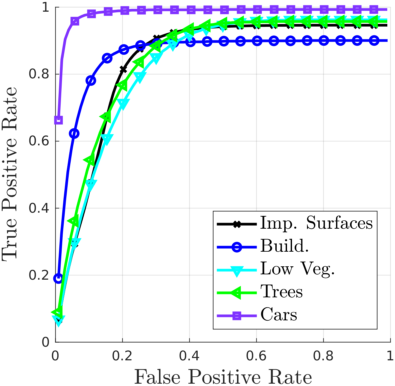
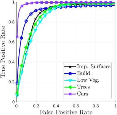
Class	IS	BU	LV	TR	CA	Mean
AUC 1px	83.53	85.53	82.59	84.37	97.64	86.73
AUC 3px	86.58	90.80	85.10	87.17	98.23	89.58

Figure 4: Average per-class ROC curves (across validation images) and average per-class AUC on the Vaihingen validation set. Prediction of the 1-pixel wide edges is a challenging problem. 3-pixel wide edges are much more accurate, in particular for spatially smooth classes. The creation of the UCM allows to cope with blurred predictions.

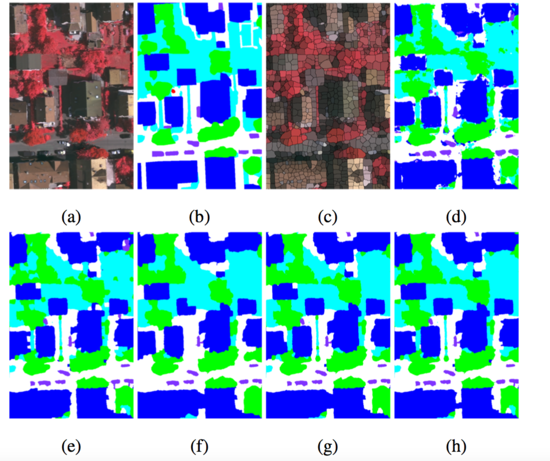
Figure 5: Examples of semantic segmentation on zoom of a validation image. (a) original image, (b) ground truth, (c) Superpixels, (d) Unary PX, (e) Unary SP, (f) CRF Color, (g) CRF Flat, (h) CRF Tree. Oversmoothing on cars (purple) is visible. However, larger and smoother structures are better delineated. (Note: in this preprint we had to decrease the graphics resolution. For full resolution, please refer to the published version, or contact the authors)

Table 1 shows numerical results obtained on the Vaihingen validation set. The proposed pipeline achieves the best overall accuracy and best F1 score compared to competitors. Unary PX and Unary SP show slightly better AA (+0.59 and +0.07, respectively) thanks to an inferior oversmoothing of small classes. The F1 scores indicate that CRF Flat and CRF Tree achieve more balanced average precision and average recall scores. Combining this observation with the fact that CRFs tend to oversmooth small classes (mostly “car”) with the F1 scores, it seems that Unary methods also tend to overpredict them, making CRF Tree achieve more balanced segmentations, i.e. better F1 scores.

Figure 5 details some examples of semantic segmentation results. It only focuses on a detail of a validation map (ID 28, upper left corner). Figure 5(c) shows the common superpixel representation obtained by the edge pooling step, which is then used to group probabilities from Unary PX into Unary SP maps (Figure 5(d) and Figure 5(e), respectively). Spatially pooling predictions in superpixels remove spurious noise and spatially smoothes class labels, as expected, which is reflected by improved or worsened class-specific accuracies, depending on the degree of smoothing beneficial to such class. Even without explicitly modeling context, maps are highly improved visually. As superpixels are generated accordingly to learned semantic boundaries, spatial pooling respects actual class borders more rather than pure color homogeneity of superpixels, as commonly implemented.

Maps generated by CRF models (Figure 5(f)-(h)) tend to switch labels for regions which are ambiguously assigned to a class. We typically observe improved segmentation across objects edges, where the Unary PX model provides spatially inhomogeneous labelings. These improvements are expected when modeling context and spatial smoothness by a CRF. The CRF Tree model (Figure 5(h) finds a good compromise between the oversmoothing offered by the CRF Color (Figure 5(f)) and the preservation of detail given by Unary SP Figure 5(e). CRF Flat seems to perform in between the two, as one would expect.

Prediction of semantic edges is accurate overall, with the tendency of being more accurate for well-defined objects (cars, buildings, trees) rather than for amorphous classes. The increase in the AUC scores from 1 pixel (1px) to 3 pixels (3px) indicates that (assuming the ground truths are precise enough) the prediction is dilated for classes that have mostly ambiguous boundaries, complex shape or wide and smooth transitions between colors and labels.

Reference	OA	AA
[35], boundary, single scale	84.8	-
[35], no boundary, ensemble	85.5	-
[35], full model	89.8	-
[34], rotation equivariant network	87.5	83.9
[44], SegNet	87.8	81.3
[3], SegNet	89.4	-
Tang, W. (Abbrev.: WUH$\_$W3) $\dagger$, ResNet-101, à-trous conv.	89.7	-
Li, H. (Abbrev.: CAS$\_$L1)$\dagger$, PSPNet	85.7	-
Sun, Y. (Abbrev.: HUSTW5)$\ddagger$ Ensemble of Deconv. Net and U-Net	91.6
Ours	84.50	82.16
Marcos et al. [34], baseline	87.4	78.2

Table 2: Comparison to state-of-the-art approaches from the literature on the ISPRS Vaihingen dataset. $\dagger$ and $\ddagger$ are taken from the ISPRS Vaihingen challenge website ranking (http://www2.isprs.org/commissions/comm2/wg4/vaihingen-2d-semantic-labeling-contest.html) as representative of recent computer vision methods, and $\ddagger$ is the current best performing method on the challenge, as per May 8, 2018. [34] baselines denotes a CNN with a number of parameters close to our VGG-derived trunk.

Table 2 shows comparison to state-of-the-art approaches. We list approaches covering different families of architectures, which in turn also provide very diverse accuracies. The best performing strategies rely on ensembling of the prediction of multiple networks, while very deep and complex segmentation approaches do improve the results, but not significantly over fully convolutional networks and standard SegNets. Our approach compares similarly to other standard fully convolutional networks. Differences are mostly visual, where our approach provides an improved spatial regularization at the cost of some oversmoothing. However, the main trunk we use (VGG) can replaced by any modern architecture in a straightforward way, and lead to improved performances without any modification to the method itself.

5.2 Zeebrugges

Color code
Model	IS	WA	CL	LV	BU	TR	BO	CA	OA	AA	F1
Unary PX	80.98	98.62	61.41	80.31	80.60	57.71	57.77	78.12	84.51	74.47	74.44
Unary SP	82.48	98.88	66.06	80.99	82.10	59.24	62.47	77.47	85.54	75.81	76.21
CRF Color	83.08	98.97	67.55	81.47	82.82	56.43	63.78	72.53	85.89	74.52	75.83
CRF Flat	83.94	98.81	67.24	80.88	84.48	48.01	60.51	72.03	86.00	71.24	74.49
CRF Tree	83.15	98.94	68.12	81.21	83.44	58.34	65.65	76.96	86.05	75.09	76.98

Table 3: Semantic segmentation accuracies on the Vaihingen validation set. F1 scores evaluate per-class accuracy. Bold denotes the best results. Models not employing CRF do not oversmooth spatially small classes (e.g. cars) by a large margin, while CRF helps in removing errors in spatially smooth structures. CRF Tree finds a good balance between these solutions.

AUC 1px	AUC 3px

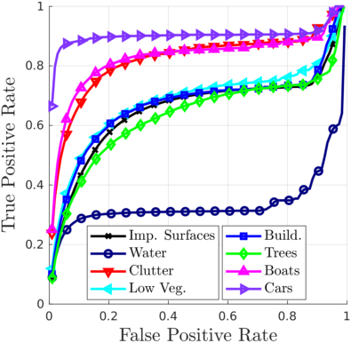
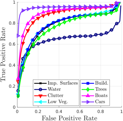
Class	IS	WA	CL	LV	BU	TR	BO	CA	Mean
AUC 1px	65.15	33.60	81.75	67.90	66.66	62.96	82.41	89.63	68.76
AUC 3px	77.67	64.50	87.80	79.05	78.60	75.78	89.75	94.64	80.97

Figure 6: Average per-class ROC curves and average per-class AUC on the Zeebrugges test set. Edge probabilities are less sharp than the Vaihingen ones (see sharp increase for the large false-positive rates), suggesting that the problem might be harder. This is also supported by the larger gap between 1- and 3-px predictions.

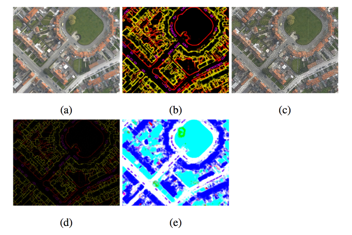
Figure 7: Example of semantic boundary detection on a test image zoom-in. (a) original image, (b) predicted edges, (c) superpixels, (d) UCM, (e) estimated class likelihoods. (Note: in this preprint we had to decrease the graphics resolution. For full resolution, please refer to the published version, or contact the authors)

The results on the Zeebrugges dataset in Table 3 reflect similar observations, with CRF Color performing slightly better on average. CRF Tree and CRF Flat provide the highest OA. In terms of AA, Unary SP still provides best numbers, since it avoids oversmoothing. However, in terms of balance between commission and omission errors (F1 score), CRF Tree outperforms all competitors, +0.77 F1 points.

Figure 7 presents a detail of the results obtained on one of the two test images. In Figure 7(b), we show edge likelihoods for three classes in a RGB composition: “impervious surfaces”, “buildings” and “cars”. On screen, the edges overlap: while the contour color for “impervious surfaces” is red, buildings are almost always contoured also by the aforementioned class, making their contour yellow (red and green). For the same reason, cars appear in purple, a composition of red and blue. Note that a given pixel can have high likelihood for more than one semantic boundary class.

It is interesting to note that the class “buildings” shows high internal variability, since the class is cluttered with edges and boundaries that are similar to actual semantic boundaries. Superpixels shown in Figure 7(c) are obtained by employing predicted edges into a watershed transform. It clearly appears that the semantic edges are more exactly followed than other boundaries, making the Unary PX pooling into Unary SP more accurate. Merging predicted edges likelihoods and superpixels edges into the UCM map (Figure 7(d)) has the effect of thinning the predicted likelihoods and making them form a segmentation tree for each class. Figure 7(e) shows the raw class likelihoods (Unary PX) the network predicts for the same area. The more saturate the color is, the more confident is the prediction.

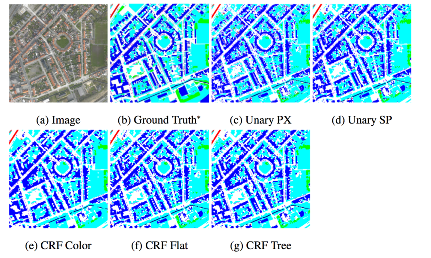
Figure 8: Example of semantic segmentation on a full Zeebrugges test image. (a) original image, (b) ground truth^∗, (c) Unary PX, (d) Unary SP, (e) CRF Color, (f) CRF Flat, (g) CRF Tree. Better viewed in the electronic version. Overall, CRF offer smoother and maps which are easier to read. Unary-derived maps are much more noisy and cluttered. ^∗The ground truth has been screen-printed from [27] and color for the “car” ground truth modified in a photo-editing software, resulting slightly blurred. (Note: in this preprint we had to decrease the graphics resolution. For full resolution, please refer to the published version, or contact the authors)

Figure 8 shows full predictions maps for the Zeebrugges test tile representing the town center. Different smoothing levels can be appreciated in particular in large semantically homogeneous regions and around object borders.

Contrarily to the Vaihingen dataset, 1px edges are not predicted well, overall. This is due to to mostly imprecise delineation of the ground truth. Although the CNN is able to learn where in a given field-of-view an edge should likely appear, at test time this results in rather smooth and fuzzy edges. Also, the variance of flat uniform surfaces (e.g. “Water”) makes the prediction of actual semantic boundaries fuzzy, an effect quantified by the large gap between 1px and 3px AUC. As for the Vaihingen benchmark, classes with relatively straight and sharp boundaries (such as “clutter”, “boats” or “cars”) are the ones delineated best. Figure 9 shows image-scale predictions of semantic edges, for each class independently.

Reference	OA	AA
[7], VGG/SVM	76.6	-
[7], AlexNet	83.3	-
[34], rotation equivariant network	82.6	75.3
RIT1$\ddagger$, [method not reported]	87.9	-
Ours	86.0	75.1

Table 4: Comparison to state-of-the-art results on the Zeebrugges challenge dataset. $\ddagger$ is the current best performing method on the challenge leaderboard, as per May 8, 2018.

Table 4 shows a comparison to available state-of-the-art results on the Zeebrugges dataset. Other approaches rely on relatively standard architectures and schemes, which are outperformed by our regularization scheme. The only notable exception is the current leader of the challenge (RIT1), but no details about the method used are currently reported. However, we note that this dataset has received less attention than the Vaihingen benchmark.

6 Discussion

The basic Unary PX and Unary SP perform really well in terms of AA. The reason is that they do not tend to oversmooth predictions and, even when Unary SP does, it oversmooths only locally in the extent of the superpixels. Since the shape of superpixels directly follows semantic boundaries in the images, average class-likelihoods in regions tend to be positively correlated with the actual label, filtering out spurious noise. Overmoothing concerns mostly spatially small classes, where CRFs tend to favor the class surrounding locally the smaller ones, missing some pixels of such objects. However, modeling spatial interactions allows to remove erroneous localizations, which is reflected by better F1 scores. For instance, accounting for relationships of class “cars” to other classes in the output space, allows to remove erroneous occurrences, such as mislabeling of car-like structures on top of buildings.

CRF are the best options. In the proposed pipeline and most baselines, CRFs are not only smoothing schemes relating on local likelihoods and color distribution but they take into account the spatial arrangement of classes (co-occurrences) together with color, deep features, relative elevation and semantic edges between them. This makes the smoothing scheme better reflect the prior information about the problem, as well as the prior knowledge acquired from training data (or possibly unrelated ancillary sources, when available). In addition, exploiting a hierarchical representation of regions further helps in smoothing only selectively, where accommodated by the energy minimization process.

The simultaneous prediction of semantic edges by the multi-task CNN seems accurate, but obviously highly correlated to the quality (and availability) of a dense ground truth used for learning. During training, the CNN seems robust to some errors in edge localization: the translation invariance property of the VGG base trunk allows the hypercolumn to contain all the relevant information to compensate for systematic shifts and biases in the ground truth. The differences between the 1px and 3px semantic edge evaluations account for these effects. In any case, edge thinning and postprocessing into superpixel edges allows for an accurate and informative UCM, impacting positively the resulting segmentation tree and the semantic segmentation overall.

Furthermore, the presented pipeline allows to use any available CNN network as the main trunk in the feature extraction network, providing the hypercolumn features. We argue that more accurate networks would provide more expressive features, leading to better segmentation quality overall. On another line, if the ground truth is limited, other schemes such as the one presented in [34] can be adopted. We posit that the presented architecture is generic and allows for data and problem specific regularization, on top of an already trained network. If the data coming from the domain specific problem (e.g. the Zeebrugges dataset) is not enough to train or properly fine tune a very deep network, it might be enough to learn multi-task layers modeling specific features of the problem with different sources of data, on top of the available architectures trained on natural images.

It is worth mentioning that we did not spend significant amount of time in fine tuning the CNN architecture and hyperparamters, nor the CRF potentials, so we assume that further improvements can be obtained by extended hyperparameters and architecture search.

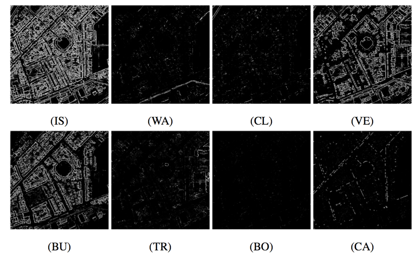
Figure 9: Per-class semantic edges on the same Zeebrugges image. Better viewed in the electronic version. Overall, structures are well delineated indicating that learning semantic boundaries in overhead imagery leads semantically coherent results (Note: in this preprint we had to decrease the graphics resolution. For full resolution, please refer to the published version, or contact the authors).

7 Conclusions and future perspectives

We proposed a model fusing bottom-up hierarchical evidence about local appearance and top-down prior information about local spatial organization and pairwise relationships between superpixels.

Regarding the first aspect, we showcased the possibility of learning the tasks of dense semantic segmentation and semantic boundaries jointly, in an end-to-end way, using a modified pretrained network. To do so, we extended a CNN formulation for multi-task learning, relying on the hypercolumn architectures built around a truncated pretrained VGG network. In our setting, we proposed to control the number of learnable parameters by forcing intermediate layers stacking into the hypercolumn to act as information bottlenecks distilling information from the original VGG activations. It results that the hypercolumn stack contains only the relevant information to solve the tasks at hand, which we assume to be less complex than vision tasks such as the ILSVRC ImageNet classification task. As the last convolutional block and the fully connected layers of the original VGG network are not dropped, the size of the network we adopted in this paper is still smaller that the full VGG. Further improvement might be gained by employing other solutions in terms of modern CNN architectures.

Regarding the second aspect, we built a CRF model specifically tailored to segment color and elevation information, with pairwise potentials accounting for the expected aspects of both data sources. We also made use of statistics collected on the training data to facilitate or to avoid specific class combinations. Thanks to the dense semantic edge likelihood, we were able to translate this information first into superpixels and then unto a segmentation tree by means of the UCM representation. We performed inference by employing the Pylon model wrapping a graph-cut solver (QPBO). Both the numerical accuracy and the overall readability of the maps were improved by injecting prior knowledge about typical layout configurations.

Future research will explore how to further simplify the segmentation map while preserving geometrical features, in order to achieve accurate vectorization and generalization without losing important details. It would be interesting to do so by specifying a generalization level e.g. corresponding to probable cuts in the segmentation tree. Another interesting research direction would be to learn pairwise potentials used in this work directly from data, since some class combinations would require more or less influence from specific potentials. This combination could be learned using structured learning, similarly to  [43].

8 References

References

- Arbelaez et al. [2011] Arbelaez, P., Maire, M., Fowlkes, C., Malik, K., 2011. Contour detection and hierarchical image segmentation. IEEE TPAMI 33 (5), 898–916.
- Asner et al. [2005] Asner, G. P., Knapp, D. E., Broadbent, E. N., Oliveira, P. J. C., Keller, M., Silva, J. N., 2005. Selective logging in the brazilian amazon. Science 310, 480.
- Audebert et al. [2018] Audebert, N., Le Saux, B., Lefèvre, S., 2018. Beyond RGB: Very high resolution urban remote sensing with multimodal deep networks. ISPRS Journal of Photogrammetry and Remote Sensing 140, 20–32.
- Besag [1974] Besag, J., 1974. Spatial interaction and the statistical analysis of lattice systems. Journal of the Royal Statistical Society. Series B 36 (2), 192–236.
- Boykov et al. [2001] Boykov, Y., Veksler, O., Zabih, R., 2001. Fast approximate energy minimization via graph cuts. IEEE Transactions on Pattern Analysis and Machine Intelligence 23 (11), 1222–1239.
- Campbell et al. [1997] Campbell, M. W., Mackeown, W. P. J., Thomas, B., Troscianko, T., 1997. Interpreting image databases by region classification. Pattern Recognition 30 (4), 555 – 563.
- Campos-Taberner et al. [2016] Campos-Taberner, M., Romero-Soriano, A., Gatta, C., Camps-Valls, G., Lagrange, A., Saux, B. L., Beaupère, A., Boulch, A., Chan-Hon-Tong, A., Herbin, S., Randrianarivo, H., Ferecatu, M., Shimoni, M., Moser, G., Tuia, D., 2016. Processing of extremely high resolution LiDAR and RGB data: Outcome of the 2015 IEEE GRSS Data Fusion Contest. Part A: 2D contest. IEEE J. Sel. Topics Appl. Earth Observ. Remote Sens. 9 (12), 5547–5559.
- Crommelinck et al. [2016] Crommelinck, S., Bennett, R., Gerke, M., Nex, F., Yang, M. Y., Vosselman, G., 2016. Review of automatic feature extraction from high-resolution optical sensor data for uav-based cadastral mapping. Remote Sensing 8 (8).
- Dollar and Zitnick [2013] Dollar, P., Zitnick, C., 2013. Structured forests for fast edge detection. In: International Conference on Computer Vision (ICCV).
- Felzenszwalb and Huttenlocher [2004] Felzenszwalb, P., Huttenlocher, D., 2004. Efficient graph-based image segmentation. International Journal of Computer Vision 59 (2), 167–181.
- Gerke [2015] Gerke, M., 2015. Use of the stair vision library within the ISPRS 2D semantic labeling benchmark (Vaihingen). Tech. rep., ITC, Univ. of Twente.
- Giménez et al. [2017] Giménez, M. G., de Jong, R., Peruta, R. D., Keller, A., Schaepman, M. E., 2017. Determination of grassland use intensity based on multi-temporal remote sensing data and ecological indicators. Remote Sensing of Environment 198, 126 – 139.
- Golipour et al. [2016] Golipour, M., Ghassemian, H., Mirzapour, F., Feb 2016. Integrating hierarchical segmentation maps with mrf prior for classification of hyperspectral images in a bayesian framework. IEEE Transactions on Geoscience and Remote Sensing 54 (2), 805–816.
- Gould et al. [2008] Gould, S., Rodgers, J., Cohen, D., Elidan, G., Koller, D., 2008. Multi-class segmentation with relative location prior. Int. J. Comp. Vision 80 (3), 300–316.
- Hariharan et al. [2011] Hariharan, B., Arbelaez, P., Bourdev, L., Maji, S., Malik, J., 2011. Semantic contours from inverse detectors. In: International Conference on Computer Vision (ICCV).
- Hariharan et al. [2015] Hariharan, B., Arbeláez, P., Girshick, R., Malik, J., 2015. Hypercolumns for object segmentation and fine-grained localization. In: IEEE/CVF International Conference on Computer Vision and Pattern Recognition.
- Hedhli et al. [2016] Hedhli, I., Moser, G., Serpico, S., Zerubia, J., 2016. A new cascade model for the hierarchical joint classification of multitemporal and multiresolution remote sensing data. IEEE Transactions on Geoscience and Remote Sensing 54 (11), 6333–6348.
- Hoberg et al. [2015] Hoberg, T., Rottensteiner, F., Queiroz-Feitosa, R., Heipke, C., 2015. Conditional random fields for multitemporal and multiscale classification of optical satellite imagery. IEEE Transactions on Geoscience and Remote Sensing 53 (2), 659–673.
- Höhle [2017] Höhle, J., 2017. Generating topographic map data from classification results. Remote Sensing 9 (3).
- Huang et al. [2017] Huang, G., Liu, Z., van der Maaten, L., Weinberger, K. Q., 2017. Densely connected convolutional networks. In: IEEE Conference on Computer Vision and Pattern Recognition (CVPR).
- Jat et al. [2008] Jat, M. K., Garg, P., Khare, D., 2008. Monitoring and modelling of urban sprawl using remote sensing and gis techniques. International Journal of Applied Earth Observation and Geoinformation 10 (1), 26 – 43.
- Kluckner et al. [2009] Kluckner, S., Mauthner, T., Roth, P. M., Bischof, H., 2009. Semantic classification in aerial imagery by integrating appearance and height information. In: ACCV 2009, Xián (China).
- Kokkinos [2016] Kokkinos, I., 2016. Pushing the boundaries of boundary detection using deep learning. In: International Conference on Learning Representations (ICLR).
- Kokkinos [2017] Kokkinos, I., 2017. In: IEEE/CVF International Conference on Computer Vision and Pattern Recognition.
- Krizhevsky et al. [2012] Krizhevsky, A., Sutskever, I., Hinton, G., 2012. ImageNet classification with deep convolutional neural networks. In: Advances in Neural Information Processing Systems.
- Lafferty et al. [2001] Lafferty, J. D., McCallum, A., Pereira, F. C. N., 2001. Conditional random fields: Probabilistic models for segmenting and labeling sequence data. In: Proceedings of the Eighteenth International Conference on Machine Learning. ICML ’01. pp. 282 – 289.
- Lagrange et al. [2015] Lagrange, A., Le Saux, B., Beaupere, A., Boulch, A., Chan-Hon-Tong, A., Herbin, S., Randrianarivo, H., Ferecatu, M., 2015. Benchmarking classification of earth-observation data: From learning explicit features to convolutional networks. In: IEEE International Geoscience and Remote Sensing Symposium. Milan, Italy, pp. 4173 – 4176.
- LeCun et al. [1998] LeCun, Y., Bottou, L., Bengio, Y., Haffner, P., 1998. Gradient-based learning applied to document recognition. Proceedings of the IEEE.
- Lempitsky et al. [2011] Lempitsky, V., Vedaldi, A., Zisserman, A., 2011. Pylon model for semantic segmentation. In: Shawe-Taylor, J., Zemel, R. S., Bartlett, P. L., Pereira, F., Weinberger, K. Q. (Eds.), Advances in Neural Information Processing Systems 24 (NIPS). pp. 1485 – 1493.
- Li et al. [2015] Li, E., Femiani, J., Xu, S., Zhang, X., Wonka, P., Aug 2015. Robust rooftop extraction from visible band images using higher order crf. IEEE Transactions on Geoscience and Remote Sensing 53 (8), 4483–4495.
- Long et al. [2015] Long, J., Shelhamer, E., Darrell, T., 2015. Fully convolutional networks for semantic segmentation. In: IEEE/CVF International Conference on Computer Vision and Pattern Recognition.
- Maggiori et al. [2017] Maggiori, E., Tarabalka, Y., Charpiat, G., Alliez, P., 2017. High-resolution aerial image labeling with convolutional neural networks. IEEE Transaction on Geoscience and Remote Sensing 55 (12), 7092 – 7103.
- Maninis et al. [2017] Maninis, K., Pont-Tuset, J., Arbeláez, P., Gool, L. V., 2017. Convolutional oriented boundaries: From image segmentation to high-level tasks. IEEE Transactions on Pattern Analysis and Machine Intelligence.
- Marcos et al. [in press] Marcos, D., Volpi, M., Kellenberger, B., Tuia, D., in press. Land cover mapping at very high resolution with rotation equivariant CNNs: towards small yet accurate models. ISPRS Journal of Photogrammetry and Remote Sensing.
- Marmanis et al. [2018] Marmanis, D., Schindler, K., Wegner, J. D., Galliani, S., Datcu, M., Stilla, U., 2018. Classification with an edge: Improving semantic image segmentation with boundary detection. ISPRS Journal of Photogrammetry and Remote Sensing 135, 158 – 172.
- Mostajabi et al. [2015] Mostajabi, M., Yadollahpour, P., Shakhnarovich, G., 2015. Feedforward semantic segmentation with zoom-out feature. In: IEEE/CVF International Conference on Computer Vision and Pattern Recognition (CVPR).
- Rother et al. [2007] Rother, C., Kolmogorov, V., Lempitsky, V., Szummer, M., 2007. Optimizing binary mrfs via extended roof duality. In: IEEE/CVF Conference on Computer Vision and Pattern Recongnition (CVPR).
- Shen et al. [2015] Shen, W., Wang, X., Wang, Y., Bai, X., Zhang, Z., 2015. Deepcontour: A deep convolutional feature learned by positive-sharing loss for contour detection. In: IEEE Conference on Computer Vision and Pattern Recognition (CVPR).
- Sherrah [2016] Sherrah, J., 2016. Fully convolutional networks for dense semantic labelling of high-resolution aerial imagery. arXiv:1606.02585.
- Shotton et al. [2006] Shotton, J., Winn, J., Rother, C., Criminisi, A., 2006. Textonboost: Joint appearance, shape and context modeling for multi-class object recognition and segmentation. In: European Conference on Computer Vision.
- Simonyan and Zisserman [2015] Simonyan, K., Zisserman, A., 2015. Very deep convolutional networks for large-scale image recognition. In: International Conference in Learning Representation. Vol. abs/1409.1.
- Uijlings and Ferrari [2015] Uijlings, J. R. R., Ferrari, V., 2015. Situational object boundary detection. In: IEEE Computer Vision and Pattern Recognition (CVPR).
- Volpi and Ferrari [2015] Volpi, M., Ferrari, V., 2015. Semantic segmentation of urban scenes by learning local class interactions. In: IEEE/CVF CVPRW Earthvision.
- Volpi and Tuia [2017] Volpi, M., Tuia, D., 2017. Dense semantic labeling of subdecimeter resolution images with convolutional neural networks. IEEE Trans. Geosci. Remote Sens. 55 (2), 881–893.
- Xie and Tu [2015] Xie, S., Tu, Z., 2015. Holistically-nested edge detection. In: IEEE/CVF International Conference on Computer Vision (CVPR).
- Zheng et al. [2017] Zheng, C., Zhang, Y., Wang, L., May 2017. Semantic segmentation of remote sensing imagery using an object-based markov random field model with auxiliary label fields. IEEE Transactions on Geoscience and Remote Sensing 55 (5), 3015–3028.
- Zhong and Wang [2007] Zhong, P., Wang, R., 2007. A multiple conditional random fields ensemble model for urban area detection in remote sensing optical images. IEEE Transaction on Geoscience and Remote Sensing 45 (12), 3978–3988.