Breakdown of the Fermi polaron description near Fermi degeneracy at unitarity

Abstract

We theoretically investigate attractive and repulsive Fermi polarons in three dimensions at finite temperature and impurity concentration through the many-body $T$-matrix theory and high-temperature virial expansion. By using the analytically continued impurity Green’s function, we calculate the direct rf spectroscopy of attractive polarons in the unitary regime. Taking the peak value of the rf spectroscopy as the polaron energy and the full width half maximum as the polaron lifetime, we determine the temperature range of validity for the quasi-particle description of Fermi polarons in the unitary limit.

1 Introduction

Understanding and exploring the properties of a moving impurity immersed in quantum many-body systems - the so-called polaron - is a fundamental problem in condensed matter physics and ultracold physics [1]. In particular, with the advent of highly controllable ultracold systems [2], the polaron problem has become a recent topic of importance in both Fermi [3, 4, 5, 6] and Bose gases [7, 8]. The use of magnetic Feshbach resonances allows for the control of the interactions between the impurity and the background system, and with the advancement of experimental apparatus the dimension of the system can be readily changed from three dimensions to two dimensions to explore the role of dimensionality [9, 10, 11].

The Fermi polaron constitutes the extreme case of a highly spin-imbalanced Fermi gas and is the conceptually simplest strongly correlated many-body system. It is thought to be a key to better understand imbalanced strongly interacting Fermi mixtures [4, 12, 13] at the crossover from a Bose-Einstein condensate (BEC) to a Bardeen-Cooper-Schrieffer (BCS) superfluid [14, 12]. Initial experimental work of Fermi polarons focused on the attractive branch [3], however there exists a higher metastable state when there is a weak two-body molecular state, known as the repulsive polaron [15, 16]. The repulsive polaron in a three-dimensional two-component Fermi gas has been recently explored in detail at the European Laboratory for Non-Linear Spectroscopy (LENS), Florence [6]. Probing the repulsive Fermi polaron may provide insight to understand repulsively interacting many-body systems such as itinerant ferromagnetism [17, 18, 19, 20].

Experimentally, both attractive and repulsive polarons have been probed through the use of radio-frequency (rf) spectroscopy [21, 22, 23], which allows the measurement of the single-particle spectral function of the polaron. The system is initially prepared with three spin states, a majority $\left|\uparrow\right\rangle$ state, and two minority states, $\left|i\right\rangle$ and $\left|f\right\rangle$, where the interaction between the majority and each minority state can be tuned. The rf spectroscopy works by applying a short rf pulse to flip the impurities into a third state, and by varying the detuning of the rf pulse, information about the single-particle excitations can be measured. For direct rf spectroscopy the third state has been tuned to be non-interacting with the $\left|\uparrow\right\rangle$ state, the strongly interacting impurities are flipped into this non-interacting state. Reverse rf spectroscopy is the opposite mechanism, the impurity-majority interaction is initially weak and the impurities are flipped into a strongly interacting third state, which allows for the full excitation spectrum to be more easily probed.

Theoretically, attractive and repulsive polarons have been extensively studied at zero temperature within a variational framework for a wide range of Fermi gases [24, 25, 26, 27, 28, 29], Bose gases [30, 31], Fermi superfluids [32, 33], and long-range interacting systems [34, 35]. Sophisticated diagrammatic quantum Monte Carlo (QMC) schemes have been developed to tackle the polaron problem [36, 37, 38, 39], with excellent agreement between the QMC simulations and many-body results. At finite but low temperature there have been few calculations for either the Fermi or Bose polaron [15, 40, 41, 42, 43], this may be in part due to the success of the variational ansatz in describing the polaron systems.

In this work, we explore the properties of the Fermi polaron in three dimensions at high temperature close to Fermi degeneracy and address the validity of the Fermi polaron description, as motivated by the on-going measurement at Massachusetts Institute of Technology (MIT) [44]. Our investigation uses a many-body $T$-matrix theory and a non-perturbative virial expansion theory [45, 46, 47, 48]. The former is a diagrammatic approach that includes pair fluctuations in the normal state and is known to well represent strongly interacting Fermi gases in the limits of spin-balance [49, 50, 51] and imbalance [52, 53, 15, 54, 55]. At zero temperature and for a single impurity, the many-body $T$-matrix and the variational ansatz are known to be equivalent in three dimensions [56, 57, 58, 59]. The latter virial expansion theory works very well at high temperature above the Fermi degenerate temperature.

It is expected that the quasi-particle and Fermi-liquid description of the polaron will break down as the temperature of the system increases and the Fermi surface broadens significantly due to thermal fluctuations [60, 61, 44]. Here, we probe the temperature breakdown of the quasi-particle description in the unitary limit, i.e. where the $s$-wave scattering length is infinite, by finding the temperature dependence of the full width half maximum (FWHM) of the rf spectra, which corresponds to the lifetime of the polaron. For temperatures above the Fermi degenerate temperature we find through the $T$-matrix and virial expansion theory a very broad peak in the rf spectra and hence the breakdown of the quasi-particle description. As the temperature lowers below the Fermi temperature the peak in the spectra becomes narrow and the FWHM becomes smaller than the polaron energy (i.e., peak position) for temperatures below $T\simeq 0.8T_{{\rm F}}$, where we will then have a defined quasi-particle.

The paper is set out as follows: in Sect. 2 we outline the many-body $T$-matrix theory and virial expansion theory for the attractive and repulsive Fermi polarons. We show how to determine the quasi-particle properties of polarons, connecting the $T$-matrix method to experimental and previous theoretical results, and briefly explain the calculation of rf spectroscopy. In Sect. 3 we explore the high temperature rf spectroscopy of the attractive polaron in the unitary limit and investigate the breakdown of the quasi-particle description. Finally, in Sect. 4 we conclude with a discussion of our results. A shows the calculation of the many-body $T$-matrix formalism and B and C are devoted to the details of the virial expansion theory.

2 Methods

We consider a highly spin-imbalanced two-component Fermi gas (i.e. $n_{\uparrow}=n\gg n_{\downarrow}$) in three dimensions that is described by the single-channel model Hamiltonian [24, 26, 62],

$$H=\sum_{\mathbf{k}}\left[\left(\varepsilon_{\mathbf{k}}-\mu\right)c_{\mathbf{k}\uparrow}^{\dagger}c_{\mathbf{k}\uparrow}+\left(\varepsilon_{\mathbf{k}}-\mu_{\downarrow}\right)c_{\mathbf{k}\downarrow}^{\dagger}c_{\mathbf{k}\downarrow}\right]+\frac{U}{V}\sum_{\mathbf{q},\mathbf{k},\mathbf{k}^{\prime}}c_{\mathbf{k}\uparrow}^{\dagger}c_{\mathbf{q}-\mathbf{k}\downarrow}^{\dagger}c_{\mathbf{q}-\mathbf{k}^{\prime}\downarrow}c_{\mathbf{k}^{\prime}\uparrow},$$ (1)

where $\varepsilon_{\mathbf{k}}\equiv\hbar^{2}\mathbf{k}^{2}/(2m)$, $\mu_{\uparrow}=\mu$ and $\mu_{\downarrow}$ are the chemical potentials of spin-up and spin-down atoms, respectively, for atoms of mass $m$, and $U<0$ is the bare attractive interatomic interaction strength. We renormalize the interaction in the usual prescription in terms of the $s$-wave scattering length $a$,

$$\frac{1}{U}=\frac{m}{4\pi\hbar^{2}a}-\sum_{\mathbf{k}}\frac{m}{\hbar^{2}\mathbf{k}^{2}}.$$ (2)

2.1 Many-body $T$-matrix theory

We start the calculation of the impurity thermal Green’s function,

$$G_{\downarrow}\left(\mathbf{k},i\omega_{m}\right)=\frac{1}{i\omega_{m}-\left(\varepsilon_{\mathbf{k}}-\mu_{\downarrow}\right)-\Sigma_{\downarrow}\left(\mathbf{k},i\omega_{m}\right)},$$ (3)

from the many-body $T$-matrix approximation, where the fermionic Matsubara frequencies are given by $\omega_{m}\equiv(2m+1)\pi/\beta$ for the inverse temperature $\beta=1/(k_{B}T)$ and any integer $m$. We take spin-down atoms as the impurities and assume that in the limit of large polarization, $x=n_{\downarrow}/n\ll 1$, the majority spin-up atoms are not affected by the interactions to a leading order approximation. Taking the majority Green’s functions as the non-interacting Green’s function,

$$G_{\uparrow}^{(0)}\left(\mathbf{k},i\omega_{m}\right)=\frac{1}{i\omega_{m}-\left(\varepsilon_{\mathbf{k}}-\mu\right)},$$ (4)

the chemical potential of the majority atoms $\mu$ as a function of temperature can then be found as $\mu^{(0)}(T)\overset{T\rightarrow 0}{\simeq}\varepsilon_{\textrm{F}}=\hbar^{2}(6\pi^{2}n)^{2/3}/(2M)$. Using the many-body T-matrix formalism set out in Appendix A, we find the analytically continued impurity Green’s function

$$G_{\downarrow}(\mathbf{k},\omega^{+})=\frac{1}{\omega^{+}-\left(\varepsilon_{\mathbf{k}}-\mu_{\downarrow}\right)-\Sigma_{\downarrow}(\mathbf{k},\omega^{+})},$$ (5)

and self energy $\Sigma_{\downarrow}(\mathbf{k},\omega^{+})$. The spectral function is found from the analytically continued Green’s function $A(\mathbf{k},\omega^{+})=-2{\rm Im}\,G(\mathbf{k},\omega^{+})$, which is given by

$$A_{\downarrow}(\mathbf{k},\omega^{+})$$

$$=\frac{{\rm Im}\,\Sigma_{\downarrow}(\mathbf{k},\omega^{+})}{(\omega^{+}-\xi_{\mathbf{k}}-{\rm Re}\,\Sigma_{\downarrow}(\mathbf{k},\omega^{+}))^{2}+({\rm Im}\,\Sigma_{\downarrow}(\mathbf{k},\omega^{+}))^{2}}.$$ (6)

The impurity chemical potential is computed self-consistently such that we find the density,

$$n_{\downarrow}=\int\frac{d\mathbf{k}}{(2\pi)^{3}}\int_{-\infty}^{\infty}\frac{d\omega}{2\pi}A_{\downarrow}(\mathbf{k},\omega)f(\omega).$$ (7)

2.2 Virial expansion theory

At high temperature, the virial expansion is a powerful tool to understand strongly-correlated many-body systems [45, 46, 47, 48], and has been found to be successful in describing the high-temperature properties of ultracold gases [63, 64]. It is an expansion in terms of the small fugacity $z_{\sigma}=e^{\beta\mu_{\sigma}}$ for each component $\sigma$. The virial expansion of the single-particle Green function in a spin-balanced Fermi gas was recently developed by Sun and Leyronas [65] and the technique was applied to investigate the Bose polaron at high temperature [66, 67]. In this work, we apply the same technique to understand the Fermi polaron at high temperature. As the theory was already well-documented by Sun et al. [65, 66, 67], here we only give a brief introduction on the essential idea and present the details in Appendix C. Following the work of Refs. [66, 67] we expand the impurity Green’s function, taking only the diagrams that do not contain any orders of the impurity fugacity, as these diagrams will contribute at a higher order.

The expansion starts from the non-interacting Green’s function in momentum space and imaginary time:

$$G_{\sigma}^{(0)}(\mathbf{k},\tau)=e^{-(\xi_{\mathbf{k}}-\mu_{\sigma})\tau}\left[-\Theta(\tau)+n_{{\rm F}}(\xi_{\mathbf{k}}-\mu_{\sigma})\right],$$ (8)

where $\Theta(\tau)$ is the Heaviside step function and $n_{{\rm F}}(x)=1/\left(e^{\beta x}+1\right)$ is the Fermi distribution. We expand the Fermi distribution in powers of the fugacity:

$$G_{\sigma}^{(0)}(\mathbf{k},\tau)=e^{\mu_{\sigma}\tau}\left[\sum_{n\geq 0}G^{(0,n)}(\mathbf{k},\tau)z_{\sigma}^{n}\right],$$ (9)

where we define

$$G^{(0,0)}(\mathbf{k},\tau) =-\Theta(\tau)e^{-\xi_{\mathbf{k}\tau}},$$ (10)

$$G^{(0,n)}(\mathbf{k},\tau) =(-1)^{n-1}e^{-\xi_{\mathbf{k}\tau}}e^{-n\beta\xi_{\mathbf{k}}}.$$ (11)

First, we note the dependence on the chemical potential $\mu_{\sigma}$ does not enter into our definition of $G^{(0,0)}$ and $G^{(0,n)}$, the chemical potential is found in the fugacity, $z_{\sigma}^{n}$, and the global $e^{\mu_{\sigma}\tau}$ factor. Because of the step function the lowest order term $G^{(0,0)}$ is retarded, and the $G^{(0,n)}$ is not retarded. When we expand the full Green’s function diagrammatically, we will in general expand free propagators that run forward, as well as some that run backward in imaginary time. A particle running backwards in imaginary time that comes in from the medium and scattering with a particle is a hole scattering process. Any diagram which involves particle-particle scattering, lines which run forward in time, we will be able to write in terms of bare $G^{(0,0)}$ at the lowest order in the fugacity. A diagram which then contains a backward running line (a hole) can then be expanded in terms of $G^{(0,n)}z_{\sigma}^{n}$, and is represented by a line with $n$ slashes.

We show in Appendix B the derivation of the thermodynamic potential to the third order of the fugacity and in Appendix C the expansion of the Green’s function in orders of the fugacity and the detailed diagrammatic construction for the impurity self-energy (i.e., Figs. 6 and 7). We use the rf spectra calculated from the virial expansion to compare with the $T$-matrix spectra in the high temperature regime.

2.3 Quasi-particle properties

Once the impurity Green’s function and chemical potential have been determined, we directly calculate the quasi-particle properties of the polaron. Near a quasi-particle excitation, we may separate the analytically continued Green’s function into two parts: a pole contribution (from quasi-particle) plus an incoherent background,

$$G_{\downarrow}=\frac{\mathcal{Z}}{\omega-\hbar^{2}\mathbf{k}^{2}/(2m^{*})+\mu_{\downarrow}-E_{P}+i\gamma/2}+\cdots,$$ (12)

where $\mathcal{Z}$ is the quasi-particle residue, $E_{P}$ is the energy of the polaron with effective mass $m^{*}$, and $\gamma$ is the decay rate of the polaron. This gives rise to a polaron spectral function $A_{\downarrow}(\mathbf{k},\omega)=-2\textrm{Im}G_{\downarrow}(\mathbf{k},\omega)$ [68, 40],

$$A_{\downarrow}\left(\mathbf{k},\omega\right)=2\pi\mathcal{Z}\delta\left(\omega+\mu_{\downarrow}-\frac{\hbar^{2}\mathbf{k}^{2}}{2m^{*}}-E_{P}\right)+\cdots.$$ (13)

The attractive and repulsive polarons are found from the poles of the Green’s function, $E_{P}=\omega_{{\rm pole}}+\mu_{\downarrow}$ [26], where the polaron energy is related to the self-energy by,

$$E_{P}= \textrm{Re}\Sigma_{\downarrow}\left(\mathbf{k}=0,E_{P}-\mu_{\downarrow}\right).$$ (14)

The spectral weight, effective mass, and decay rate are given by

$$\mathcal{Z} = \left.\left(1-\frac{\partial\mathbf{\textrm{Re}}\Sigma_{\downarrow}}{\partial\omega}\right)^{-1}\right|_{\mathbf{k}=0,\omega=\omega_{{\rm pole}}},$$ (15)

$$\frac{m}{m^{*}} = \left.\left(1+\frac{\partial\mathbf{\textrm{Re}}\Sigma_{\downarrow}}{\partial\varepsilon_{\mathbf{k}}}\right)\left(1-\frac{\partial\mathbf{\textrm{Re}}\Sigma_{\downarrow}}{\partial\omega}\right)^{-1}\right|_{\mathbf{k}=0,\omega=\omega_{{\rm pole}}},$$ (16)

$$\gamma = -2\mathcal{Z}\textrm{Im}\Sigma_{\downarrow}(0,\omega_{{\rm pole}}).$$ (17)

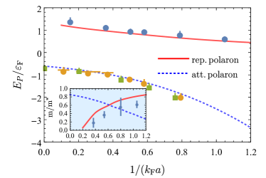
Figure 1: The attractive (lower branch) and repulsive (upper branch) polaron energies as a function of the interaction strength for an impurity density $x\equiv n_{\downarrow}/n=0.01$ and temperature $T=0.03T_{{\rm F}}$. We show for comparison the experimental results from Ref. [6] (circular symbols) and the results from Ref. [3] (square symbols). The inset shows the inverse effective mass of the repulsive polaron (solid red), attractive polaron (blue dashed), and experimental results Ref. [6] (circular symbols).

As an example of the quasi-particle properties of the analytically continued Green’s function we show the attractive and repulsive polaron energies in Fig. 1 found from Eq. (14) using the many-body $T$-matrix theory. Fixing the temperature to effectively zero, $T=0.03T_{{\rm F}}(\equiv\varepsilon_{\textrm{F}}/k_{B})$, and the impurity density to $x=0.01$ we show the attractive (lower branch) and repulsive (upper branch) polaron energies as a function of the dimensionless interaction strength $(k_{\textrm{F}}a)^{-1}$, where $k_{\textrm{F}}=(3\pi^{2}n)^{1/3}$. We find a reasonable agreement with the experiments of Ref. [3] (square symbols) and Ref. [6] (circular symbols), as has been found in previous works, for both the attractive and repulsive polarons [58, 42]. For the repulsive branch, our calculations do not attempt to find the polaron energy below a threshold interaction strength of $(k_{{\rm F}}a)^{-1}=0.1$ [59, 42]. The inset shows the effective mass for the attractive (blue dashed) and repulsive (red solid) polarons. We see that for the repulsive polaron the effective mass is consistently over-estimated for all interaction strengths compared to the experimental results. The over-estimation in the predicted effective mass at zero temperature was noted earlier in Ref. [6].

2.4 Radio-frequency spectroscopy

The single-particle properties of the polaron can be experimentally probed with radio-frequency (rf) spectroscopy [69, 23], which has been used in experiments to find the energy, effective mass, and residue of the attractive and repulsive polarons [3, 6, 9, 10]. Theoretically, by calculating the rf spectra we can connect our many-body $T$-matrix results of the quasi-particle properties of the polaron at finite temperature and impurity density directly to the experimentally observed rf spectra. With our knowledge of the spectral function in Eq. (6), we calculate the direct rf and reverse rf spectroscopy of the polaron and find the position of the maximum of the peaks, which corresponds to the attractive and repulsive polaron energies, and the full width half maximum, which can be viewed as the lifetime of the polaron.

We consider a three-component Fermi gas with the majority $\left|\uparrow\right\rangle$ component and minority components $\left|i\right\rangle$ and $\left|f\right\rangle$. Within the linear response frame work the transition from an initial to final state is [70, 53, 71, 72, 73, 74],

$$I(\omega_{{\rm rf}})=2\Omega^{2}{\rm Im}\,\chi(\mathbf{k}=0,\mu_{f}-\mu_{i}-\omega_{{\rm rf}}),$$ (18)

where $\Omega$ is the Rabi frequency, $\mu_{i}$ and $\mu_{f}$ are the initial and final state chemical potentials, and $\omega_{{\rm rf}}$ is the rf frequency. At finite temperature the retarded correlation function is found from the time-ordered correlation function,

$$\chi(\mathbf{r},\mathbf{r}^{\prime},\tau)=\langle T_{\tau}\psi_{f}^{\dagger}(\mathbf{r},\tau)\psi_{i}(\mathbf{r},\tau)\psi_{f}(\mathbf{r},0)\psi_{i}^{\dagger}(\mathbf{r},0)\rangle.$$ (19)

The calculation of the analytically continued correlation function contains several different diagrammatic contributions [72, 59], for our calculation we will assume there are no final state interactions and ignore the higher order vertex corrections [75, 76]. The spectral response function in the domain of Matsubara frequencies then becomes

$$\chi(i\nu_{n})=\frac{1}{\beta}\sum_{i\omega_{m}}\int\frac{d\mathbf{k}}{(2\pi)^{3}}G_{f}(\mathbf{k},i\omega_{m})G_{i}(\mathbf{k},i\nu_{n}+i\omega_{m})$$ (20)

and the rf response on the real axis is

$$I(\omega)= \Omega^{2}\int\frac{d\mathbf{k}}{(2\pi)^{3}}\int\frac{d\varepsilon}{2\pi}f(\varepsilon)A_{f}(\mathbf{k},\varepsilon+\omega+\mu_{i}-\mu_{f})A_{i}(\mathbf{k},\varepsilon).$$ (21)

Here, $A_{\sigma}(\mathbf{q},\omega)$ corresponds to the spectral function of the state $\sigma$. In the calculation of the rf spectra we ignore the occupation of the final state, however at finite temperature the occupation is, in principle, non-zero. Taking the final state to then become $A_{f}(\mathbf{q},\omega)=2\pi\delta(\omega-\varepsilon_{\mathbf{q}}+\mu_{f})$ and the initial state to be the minority the direct rf spectroscopy is given by

$$I(\omega)=-\Omega^{2}\int\frac{d\mathbf{k}}{(2\pi)^{3}}f(\varepsilon_{\mathbf{k}}-\mu_{\downarrow}-\omega)A_{\downarrow}(\mathbf{k},\varepsilon_{\mathbf{k}}-\mu_{\downarrow}-\omega).$$ (22)

The reverse rf spectroscopy is given by flipping the spins from an initial non-interacting state to a final state which is strongly interacting, i.e. the unoccupied minority state,

$$I(\omega)=-\Omega^{2}\int\frac{d\mathbf{k}}{(2\pi)^{3}}f(\varepsilon_{\mathbf{k}}-\mu_{i})A_{\downarrow}(\mathbf{k},\varepsilon_{\mathbf{k}}-\mu_{\downarrow}+\omega).$$ (23)

where $\mu_{i}$ can be determined from the non-interacting impurity in state $\left|i\right\rangle$ and the final chemical potential in the spin-flipped state $\left|f\right\rangle$ is $\mu_{\downarrow}$. As a check to our calculation of the direct rf spectra we can calculate the number density, i.e.

$$n_{\downarrow}=\int\frac{d\omega}{2\pi}I(\omega),$$ (24)

which holds if we set the Rabi frequency $\Omega=1$.

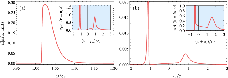
Figure 2: (a) The direct rf spectroscopy in arbitrary units for an interaction strength of $1/(k_{{\rm F}}a)=0.4$, an impurity concentration $x=0.01$ and temperature $T=0.03T_{{\rm F}}$. (b) The reverse rf spectroscopy at the same condition. The two insets plot the corresponding dimensionless spectral function at zero momentum, $A_{\downarrow}(\mathbf{k}=0,\omega)$, and at the Fermi momentum, $A_{\downarrow}(\mathbf{k}=k_{{\rm F}},\omega)$.

As an example of the two rf spectroscopy schemes we plot in Fig. 2(a) the direct rf spectra and in Fig. 2(b) the reverse rf spectra for an interaction strength of $1/(k_{{\rm F}}a)=0.4$, impurity concentration $x=0.01$, and temperature $T=0.03T_{{\rm F}}$, calculated by using the many-body $T$-matrix theory. The peak value in the direct spectrum corresponds to the attractive polaron energy (more precisely, $-E_{P}$). For the reverse rf spectroscopy the repulsive polaron is found from the positive peak and the peak at negative frequencies is the attractive polaron energy. We see in both spectra the attractive polaron peak is asymmetric and for the reverse rf scheme the peak at positive frequency is significantly broader, indicating the finite lifetime of the repulsive polaron. The polaron energies are the same as those found in Fig. 1 with the quasi-particle description, as expected.

The two insets show the spectral function calculated at zero momentum and the Fermi momentum, respectively, and we see how the spectral weight shifts from the negative peak to the positive energy peak as the momentum increases. Going from $k=0$ to $k=k_{\rm F}$, both peaks shift up in energy by an amount comparable to the polarons’ kinetic energies, $(m/m^{*})E_{\rm F}$, where $(m/m^{*})$ for the attractive and repulsive branches may be read out from the inset of Fig. 1 ($\simeq 0.7$ for the attractive polaron and $\simeq 0.4$ for the repulsive polaron). For the spectral functions and the reverse spectra in Fig. 2 (b) we have added a finite width with a small imaginary part to make the sharp peaks of the attractive polaron visible.

At zero temperature and for a single impurity we expect the attractive polaron energy from the rf spectroscopy to be a sharp $\delta$-function peak; the rf pulse provides the energy required to excite the polaron into the final state. As the temperature and impurity density increases, the width of the rf spectra increases due to the finite number of states which are now occupied in the spectral function of the imbalanced gas. Within the $T$-matrix scheme considered here we need a finite impurity population and the lowest temperature we can consider is $T=0.03T_{{\rm F}}$, and we expect the spectra to have a finite asymmetrical width which shifts the energy of the polaron. As the temperature and impurity increases we expect the widths and peak positions of the two rf spectroscopy schemes to change by differing amounts, i.e. we do not expect the temperature and impurity dependence to be the same.

3 Fermi polaron near Fermi degeneracy at unitarity

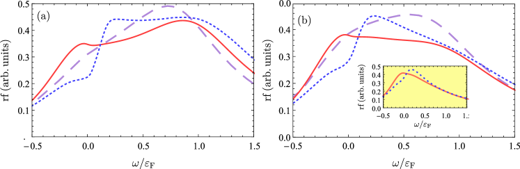
Figure 3: Direct rf spectroscopy from the second (red solid), third (blue dotted) virial expansion, and $T$-matrix (purple dashed) at the interaction strength $1/(k_{{\rm F}}a)=0$ for temperatures in (a) $T=1.25T_{{\rm F}}$ and (b) $T=1.5T_{{\rm F}}$. Insert: rf spectroscopy comparing the second and third virial expansion at the temperature $T=2.0T_{{\rm F}}$.

In the high temperature regime we expect the quasi-particle description of the polaron to break down and determining this transition temperature is non-trivial. Motivated by recent experiments at MIT [44], we explore the breakdown of the attractive polaron in the unitary limit as a function of temperature using the spectral function calculated from the $T$-matrix theory. We calculate the attractive polaron energy from the peak value of the rf spectra and the lifetime of the quasi-particle excitation from the FWHM [3, 44].

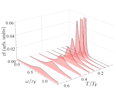
Figure 4: Direct rf spectroscopy in arbitrary units from the $T$-matrix Green’s function at $1/(k_{{\rm F}}a)=0$ for temperatures from $T=0.1T_{{\rm F}}$ to $T=0.7T_{{\rm F}}$ as a function of rf pulse $\omega/\varepsilon_{{\rm F}}$.

In Fig. 3 we plot the direct rf spectroscopy from the $T$-matrix (purple dashed) spectral function and the high temperature virial expansion calculated at the second (red solid) and third order (blue dotted) at two temperatures (a) $T=1.25T_{{\rm F}}$ and (b) $T=1.5T_{{\rm F}}$, for the interaction strength $1/(k_{{\rm F}}a)=0$ and the finite impurity density $x=0.1$ [44]. We see in Fig. 3(a) that for all three spectra there is a peak at finite rf frequency suggesting the formation of a quasi-particle with finite energy. However, the peaks are very broad and asymmetrical, indicating that a quasi-particle is not well defined. There are additional structures in the virial spectra, i.e., the large asymmetry between the peaks and the sharp increase in the third order at $\omega\simeq 0$. We attribute them to the finite number of terms in the expansion of the virial Green’s function; in the strongly interacting regime physics of more than three-body contributions will play a significant role. As we go to higher temperature, $T=1.5T_{{\rm F}}$ in Fig. 3(b) the peak at finite rf frequency is transferred to the peak at $\omega\simeq 0$ for all three spectra, and the system is becoming weakly interacting. The inset in Fig. 3 shows the second and third virial spectra at the temperature $T=2T_{{\rm F}}$. The two peaks have merged into a single peak at $\omega\simeq 0$, indicating that there is no longer any quasi-particle in the system and it is weakly interacting.

For temperatures below the Fermi temperature, $T=T_{{\rm F}}$, we expect the virial and $T$-matrix spectra will qualitatively give the same behavior, however, the virial expansion is expected to break down as the temperature is lowered and the fugacity becomes larger. There is no definite method to define a threshold temperature at which the expansion has broken down. We see in the calculation of the Green’s function at the third order, the spectral function becomes unphysical for values of fugacity $z_{\downarrow}\geq 0.3$ ($T\simeq 1.25T_{{\rm F}}$), where the spectral function becomes negative for some values of $\omega$ at small momenta. We expect that this will be canceled off by higher order terms in the virial expansion, and we take this temperature as a lower-bound for the validity of the virial expansion.

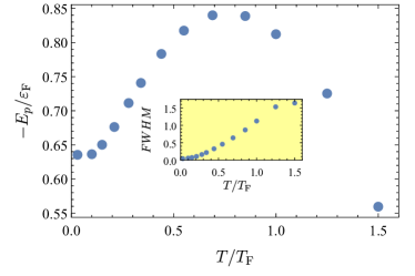
Figure 5: The temperature dependence of the attractive polaron energy at unitarity for the impurity concentration $x=0.1$ from the peak position of the rf spectra. The inset shows the full width half maximum in units of $\varepsilon_{F}$.

Moving to the low temperature regime, in Fig. 4 we show the temperature evolution of the rf spectra calculated from the $T$-matrix theory at temperatures from $T=0.1T_{{\rm F}}$ to $T=0.7T_{{\rm F}}$ and at the impurity concentration of $x=0.1$ [44]. We clearly see that there remains a definite peak and the spectra broaden as the temperature increases. We extract the peak values of the spectra and the FWHM and plot them in Fig. 5. We find that the polaron energy $-E_{P}$ increases and has a maximum around $T\simeq 0.8T_{{\rm F}}$ as the attraction between polaron and the medium increases. The energy of the polaron then decreases for temperatures above $T\simeq 0.8T_{{\rm F}}$ as the the FWHM becomes on the order of the Fermi energy and the Fermi surface broadens. For low temperatures the FWHM is increasing approximately as $(T/T_{{\rm F}})^{2}$ and becomes greater than the polaron energy at temperatures $T>0.8T_{{\rm F}}$. We propose that the quasi-particles are well defined if their inverse lifetime is less than their excitation energy. Thus, we conclude that the attractive polaron in the unitary limit remains well defined up to temperatures of about $T\simeq 0.8T_{{\rm F}}$.

4 Conclusion

In summary, using the many-body $T$-matrix approximation and high temperature virial expansion, we have calculated the direct rf spectroscopy for a range of temperatures at unitarity and discussed the breakdown of the quasi-particle description of the attractive polaron as temperature increases. In the high temperature regime, where the virial expansion is valid, we found qualitative agreement between the rf spectra obtained from the $T$-matrix scheme and virial expansion, showing the failure of the quasi-particle description. In the low temperature regime, where the $T$-matrix theory is reliable, we have calculated the FWHM of the rf spectra and have found that the quasi-particle description is well defined for temperatures below $T\simeq 0.8T_{{\rm F}}$, where the FWHM becomes smaller than the absolute value of the polaron energy.

Appendix A Many-body T-matrix

To use the well-established many-body $T$-matrix theory to find the impurity Green’s function $G_{\downarrow}\left(\mathbf{k},i\omega_{m}\right)$ [78, 62, 79, 50], we sum all of the ladder-type diagrams, and obtain the self-energy,

$$\Sigma_{\downarrow}=k_{B}T\sum_{\mathbf{q},i\nu_{n}}G_{\uparrow}^{(0)}\left(\mathbf{q}-\mathbf{k},i\nu_{n}-i\omega_{m}\right)\Gamma\left(\mathbf{q},i\nu_{n}\right),$$ (25)

where the vertex function $\Gamma$ can be written through the Bethe-Salpeter equations,

$$\Gamma\left(\mathbf{q},i\nu_{n}\right)=\frac{1}{U^{-1}+\chi\left(\mathbf{q},i\nu_{n}\right)},$$ (26)

with the pair propagator $\chi(\mathbf{q},i\nu_{n})$,

$$\chi=k_{B}T\sum_{\mathbf{k},i\omega_{m}}G_{\uparrow}^{(0)}\left(\mathbf{q}-\mathbf{k},i\nu_{n}-i\omega_{m}\right)G_{\downarrow}^{(0)}\left(\mathbf{k},i\omega_{m}\right),$$ (27)

and the bosonic Matsubara frequencies, $\nu_{n}\equiv 2n\pi/\beta$, for integer $n$.

The closed set of equations, (3) to (27), can be solved directly with Matsubara frequencies [40]. Alternatively, we can analytically continue the Matsubara frequencies to the real axis. This will allow us to calculate the spectral function without numerically continuing to real frequencies [52]. The analytically continued impurity Green’s function is given by

$$G_{\downarrow}(\mathbf{k},\omega^{+})=\frac{1}{\omega^{+}-\left(\varepsilon_{\mathbf{k}}-\mu_{\downarrow}\right)-\Sigma_{\downarrow}(\mathbf{k},\omega^{+})},$$ (28)

where $\omega^{+}\equiv\omega+i0^{+}$ and the self-energy function now takes the form [80],

$$\Sigma_{\downarrow} (\mathbf{k},\omega^{+})=$$

$$\int\frac{d\mathbf{q}}{(2\pi)^{3}}\frac{d\varepsilon}{\pi}\biggl{[}b(\varepsilon)G_{\uparrow}^{(0)}(\mathbf{k}-\mathbf{q},\varepsilon-\omega^{+}){\rm Im}\Gamma(\mathbf{q},\varepsilon^{+})$$

$$-f(\varepsilon){\rm Im}G_{\uparrow}^{(0)}(\mathbf{k},\varepsilon^{+})\Gamma(\mathbf{k}+\mathbf{q},\varepsilon+\omega^{+})\biggl{]},$$ (29)

where $f(z)=(\exp(\beta z)+1)^{-1}$ and $b(z)=(\exp(\beta z)-1)^{-1}$ are the Fermi and Bose distributions respectively . Performing the Matsubara sum analytically the vertex function is given by

$$\Gamma^{-1} \left(\mathbf{q},\omega^{+}\right)$$

$$=\frac{m}{4\pi a}-\sum_{\mathbf{k}}\left[\frac{1-f(\xi_{\mathbf{k}+\mathbf{q}/2}^{\uparrow})-f(\xi_{\mathbf{k}-\mathbf{q}/2}^{\downarrow})}{\omega^{+}-\xi_{\mathbf{k}-\mathbf{q}/2}^{\uparrow}-\xi_{\mathbf{k}+\mathbf{q}/2}^{\downarrow}}+\frac{1}{2\varepsilon_{\mathbf{k}}}\right],$$ (30)

where $\xi_{\mathbf{k}}^{\sigma}=\varepsilon_{\mathbf{k}}-\mu_{\sigma}$. We then find the imaginary part of the analytically continued self-energy,

$${\rm Im}\,\Sigma_{\downarrow}(\mathbf{k},\omega)= \int\frac{d^{3}q}{(2\pi)^{3}}\frac{d\varepsilon}{2\pi}\left(b(\varepsilon)+f(\varepsilon-\omega)\right)$$

$$\times{\rm Im}\Gamma(\mathbf{q},\varepsilon)\,{\rm Im}G_{\uparrow}^{(0)}(\mathbf{q}-\mathbf{k},\varepsilon-\omega),$$ (31)

and we calculate the real part of the self-energy from the Kramers-Kronig relation,

$${\rm Re}\,\left[f(z)\right]=\frac{1}{\pi}\mathcal{P}\int_{-\infty}^{\infty}dz^{\prime}\frac{{\rm Im}\left[f(z^{\prime})\right]}{z^{\prime}-z},$$ (32)

which gives,

$${\rm Re}\,\Sigma {}_{\downarrow}(\mathbf{k},\omega)=$$

$$\int\frac{d^{3}q}{(2\pi)^{3}}\frac{d\varepsilon}{2\pi}\bigg{[}-{\rm Im}\Gamma(\mathbf{q},\varepsilon){\rm Re}G_{\uparrow}^{(0)}(\mathbf{q}-\mathbf{k},\varepsilon-\omega^{+})b(\varepsilon)$$

$$+{\rm Re}\Gamma(\mathbf{q},\varepsilon){\rm Im}G_{\uparrow}^{(0)}(\mathbf{q}-\mathbf{k},\varepsilon-\omega^{+})f(\varepsilon-\omega)\bigg{]}.$$ (33)

The above procedure for calculating the impurity Green’s function and vertex function breaks down for either a critical interaction strength, temperature, or impurity concentration, when there exists a tightly bound molecular state. For a balanced gas this is the condensation of spontaneously created molecules and is the Thouless criterion for superfluidity [81],

$$\Gamma^{-1}\left(\mathbf{q}=0,i\nu_{n}=0\right)=0,$$ (34)

In this work we only consider the regimes away from the respective molecular transitions.

Appendix B Virial expansion of an imbalanced Fermi gas

Following the derivation of the imbalanced thermodynamic potential by Refs. [82, 48], we write it in the following third order form,

$$\Omega=\Omega^{(1)}-k_{B}T\frac{2}{\lambda^{3}}\left[z_{\uparrow}z_{\downarrow}\Delta b_{2}+\frac{z_{\uparrow}^{2}z_{\downarrow}+z_{\uparrow}z_{\downarrow}^{2}}{2}\Delta b_{3}\right],$$ (35)

where $\Omega^{(1)}=\Omega^{(1)}(\mu_{\uparrow})+\Omega^{(1)}(\mu_{\downarrow})$ are the thermodynamic potential of a non-interacting Fermi gas for each spin component and the thermal wavelength is $\lambda=\sqrt{2\pi/mk_{\rm B}T}$. The second order virial coefficient $\Delta b_{2}$ can be straight forwardly calculated [83], and unitarity is given by $\Delta b_{2}=1/\sqrt{2}$. The third order virial coefficient $\Delta b_{3}$ can be found through a summation over energies of the scattered states [45, 84] or through field theoretical method [85, 47, 46], and at unitarity $\Delta b_{3}=-0.35501\dots$.

With the virial expansion of the thermodynamic potential we can find the density of each spin component, $n_{\sigma}=-\partial\Omega/\partial\mu_{\sigma}$. We solve the majority chemical potential as in the finite temperature $T$-matrix calculation, from the ideal gas at the same temperature, and calculate the minority for a given density $x=n_{\downarrow}/n_{\uparrow}$. In 3D $\tau=T/T_{{\rm F}}$ and $T_{{\rm F}}=\hbar^{2}(6\pi^{2}n)^{2/3}/2m/k_{B}$ is the Fermi temperature and we can find the dimensionless density $\tilde{n}=n\lambda^{3}/2=4/(6\sqrt{\pi}\tau^{3/2})$

$$\tilde{n}_{\uparrow} =\tilde{n}_{\uparrow}^{(1)}(z_{\uparrow})$$ (36)

$$\tilde{n}_{\downarrow} =\tilde{n}_{\downarrow}^{(1)}(z_{\uparrow})+z_{\uparrow}z_{\downarrow}2\Delta b_{2}+\left(z_{\uparrow}^{2}z_{\downarrow}+2z_{\uparrow}z_{\downarrow}^{2}\right)\Delta b_{3},$$ (37)

where the ideal density is given by $\tilde{n}_{\sigma}^{(1)}(z)=(2/\sqrt{\pi})\int_{0}^{\infty}\sqrt{t}\left[ze^{-t}/(1+ze^{-t})\right]dt$.

Appendix C Virial expansion of Green’s function

The virial expansion can be used to expand the self-energy in orders of the non-interacting Green’s function in powers of the fugacity [47, 86, 87, 65, 88, 89, 90, 66]. For our highly imbalanced system we will utilize the fact that the minority component chemical potential will always be large and negative and the fugacity will be small. To begin then, we will only look at diagrams with $O(z_{\downarrow}^{0})$ within the usual expansion of the self-energy.

Figure 6: (a) The lowest order contribution to the self-energy for the spin $\downarrow$ minority Green’s function, where $T_{2}$ is the two-body T-matrix. (b) The third order, $O(z_{\downarrow}^{2})$, contribution where the hole line is double slashed.

C.1 Second-order self energy

The first term to contribute to the $\downarrow$ minority Green’s function is shown in Fig. 6(a). The analytical expression for the above diagram is given by:

$$\Sigma_{\downarrow}^{(1)}(k,\tau)=z_{\uparrow}\int\frac{d\mathbf{P}}{(2\pi)^{3}}e^{\mu_{\downarrow}\tau}e^{-(\beta-\tau)\xi_{\mathbf{P}-\mathbf{k}}}T_{2}(P,\tau),$$ (38)

and the two-body T-matrix, $T_{2}(P,\tau)=e^{-\tau P^{2}/4m}T_{2}(0,\tau)$, is the inverse Laplace transform of the two-body T-matrix, $t_{2}(s)=(4\pi/m)\left[a^{-1}-\sqrt{-ms}\right]^{-1}$,

$$T_{2}(0,\tau)=\int_{C_{\gamma}}\frac{ds}{2\pi i}e^{-\tau s}t_{2}(s).$$ (39)

The inverse Laplace transform is defined as a contour integral on the Bromwich contour, which is a straight line in the complex plane parallel to the imaginary axis and such that all of the function is analytic to the left of the contour. It is clear from the definition of $t_{2}(s)$ that there is a branch cut for all positive $s$ and so we can take the Bromwich contour to be the positive real axis, and if $a^{-1}<0$ include the additional contribution from the residue due to the bound state contribution.

So we have,

$$T_{2}(0,\tau)=-\Theta(a^{-1})\frac{8\pi e^{E_{b}\tau}}{m^{2}a}-\frac{4}{m^{3/2}}\int_{0}^{\infty}dxe^{-\tau x}\frac{\sqrt{x}}{x+E_{b}},$$ (40)

where $E_{b}=1/(ma^{2})$. Combining all of the above and taking the Fourier transform for the imaginary time to Matsubara frequencies we arrive at to $O(z_{\downarrow}^{0})$

$$\Sigma_{\downarrow}^{(1)} (k,i\omega_{n})$$

$$=z_{\uparrow}\int_{0}^{\infty}d\tau e^{i\omega_{n}\tau}\int\frac{d\mathbf{P}}{(2\pi)^{3}}e^{\mu_{\downarrow}\tau}e^{-(\beta-\tau)\xi_{\mathbf{P}-\mathbf{k}}}T_{2}(P,\tau),$$

$$=z_{\uparrow}F(k,i\omega_{n}+\mu_{\downarrow}),$$ (41)

where,

$$F(k,\omega^{+}) =\int\frac{d\mathbf{P}}{(2\pi)^{3}}e^{-\beta\frac{(\mathbf{P}-\mathbf{k})^{2}}{2m}}\left[\int_{0}^{\infty}dx\frac{\rho_{2}(x)}{E^{+}-\frac{P^{2}}{4m}-x+\frac{(\mathbf{P}-\mathbf{k})^{2}}{2m}}+\frac{8\pi}{m^{2}a}\Theta(a^{-1})\frac{1}{\omega-\frac{P^{2}}{4m}-E_{b}+\frac{(\mathbf{P}-\mathbf{k})^{2}}{2m}}\right],$$ (42)

We have analytically continued the Matsubara frequencies to the real axis as there are no more poles in the upper-complex plane. There is an additional higher order, $O(z_{\downarrow})$, contribution to $\Sigma_{\downarrow}^{(1)}(\mathbf{k},\omega)$ [65] and we omit its contribution here.

Figure 7: The two diagrams for the spin $\downarrow$ self-energy, where $T_{3}$ is the three-body T-matrix and $T_{2}$ is the two-body T-matrix.

C.2 Third-order self energy

For the third order contributions we follow the calculation of the diagrams from Refs. [65, 66], where for a two-component Fermi gas there are six diagrams which contribute to the third order self-energy. For every slashed line we have a power of fugacity (and there will be an additional $e^{\mu_{\sigma}\tau}$ with the three body STM-equations $T_{3}^{\sigma}$), we can see that to zeroth order in the minority fugacity, only the diagrams in Fig. 7(a) and (b) will contribute. There is also an additional contribution at the same order of the fugacity by slashing the second order diagram twice that is found in Fig. 6(b).

The first contribution to the third order self energy we calculate is the double slashed diagram in Fig. 6(b). The contribution is obtained from $\Sigma^{(1)}$ by changing $G^{(0,1)}$ to $G^{(0,2)}$ and multiplying by a factor of $z_{\uparrow}$. The analytically continued contribution is given by,

$$\Sigma {}_{\downarrow}^{(2,1)}(k,\omega^{+})$$

$$=-z_{\uparrow}^{2}\int\frac{d\mathbf{P}}{(2\pi)^{3}}\int dx\frac{e^{-\beta\frac{(\mathbf{P}-\mathbf{k})^{2}}{m}}\rho_{2}(x)}{\omega^{+}+\mu_{\downarrow}-\left(\frac{P^{2}}{4m}+x+\frac{(\mathbf{P}-\mathbf{k})^{2}}{2m}\right)},$$ (44)

where again we have analytically continued to the real axis. The third order diagrams in Fig. 7 give the following contributions [65],

$$\Sigma_{\downarrow}^{(2,2)}(k,\omega^{+})= z_{\uparrow}^{2}\int\frac{d\mathbf{P}d\mathbf{p}_{1}}{(2\pi)^{6}}\int_{0}^{\infty}dx\rho_{3}(\mathbf{p}_{1},\mathbf{p}_{1};x)\frac{e^{-\beta\left[\frac{(3\mathbf{p}_{1}+\mathbf{P}+\frac{(\mathbf{P}-\mathbf{k})^{2}}{2m})^{2}}{8m}\right]}}{\omega^{+}+\mu_{\downarrow}+\frac{P^{2}}{6m}+\frac{(\mathbf{P}-\mathbf{k})^{2}}{2m}-\frac{3(\mathbf{p}_{1}+\mathbf{P})^{2}}{8m}}$$

$$+ z_{\uparrow}^{2}\int\frac{d\mathbf{P}d\mathbf{p}_{1}}{(2\pi)^{6}}\int_{0}^{\infty}dx\tilde{\rho}_{3}(\mathbf{p}_{1},\mathbf{p}_{2};x)\frac{e^{-\beta\left[\frac{(3\mathbf{p}_{1}+\mathbf{P}+\frac{(\mathbf{P}-\mathbf{k})^{2}}{2m})^{2}}{8m}\right]}}{\omega^{+}+\mu_{\downarrow}+\frac{P^{2}}{6m}+\frac{(\mathbf{P}-\mathbf{k})^{2}}{2m}-\frac{3(\mathbf{p}_{1}+\mathbf{P})^{2}}{8m}}$$ (45)

where we define

$$\rho_{3}(\mathbf{p}_{1},\mathbf{p}_{2};x)=\frac{1}{2\pi i}\biggl{[} t_{2}\left(x+i\delta-\frac{3p_{1}^{2}}{4m}\right)t_{3}(\mathbf{p}_{1},\mathbf{p}_{2};x+i\delta)t_{2}\left(x+i\delta-\frac{3p_{2}^{2}}{4m}\right)$$

$$-t_{2}\left(x-i\delta-\frac{3p_{1}^{2}}{4m}\right)t_{3}(\mathbf{p}_{1},\mathbf{p}_{2};x-i\delta)t_{2}\left(x-i\delta-\frac{3p_{2}^{2}}{4m}\right)\biggl{]},$$ (46)

and $\tilde{\rho}_{3}$ is defined where the three-body T-matrix $t_{3}$ has removed a non one-particle irreducible contribution,

$$\tilde{t}_{3}(\mathbf{p}_{1},\mathbf{p}_{2};s)=t_{3}(\mathbf{p}_{1},\mathbf{p}_{2};s)-\frac{1}{\frac{p_{1}^{2}+p_{2}^{2}}{m}+\frac{\mathbf{p}_{1}\cdot\mathbf{p}_{2}}{m}-s}.$$ (47)

The three-body integral equations $t_{3}(\mathbf{p}_{1},\mathbf{p}_{2};s)$ are defined in Appendix D. In the numerical calculation we add a small imaginary part $\delta$ to deal with the poles and branch cuts in the STM equations, we find this gives a small, but negligible, shift to the final contribution to the self-energy. In total to third order, for an imbalanced gas, we can see that the third order contribution to the self energy is,

$$\Sigma_{\downarrow}^{(3)}(k,\omega)=\Sigma_{\downarrow}^{(2,1)}(k,\omega)+\Sigma_{\downarrow}^{(2,2)}(k,\omega)$$ (48)

Appendix D Three body-integral equations

In the calculation of the self-energy to third order, i.e. $O(z_{\uparrow}^{2})$, we need to calculate the vacuum three-body $T_{3}$ matrix, which can be found from the Skornaikov-Ter Martirosian (STM) integral equation [91]. Following the standard approach of the diagrammatic three-body scattering $T_{3}$ matrix for an $\uparrow\uparrow\downarrow$ system [92, 93, 47, 90], we have

$$T_{3} (p_{1},p_{2};P)=-G_{\downarrow}(P-p_{1}-p_{2})-$$

$$\sum_{q}G_{\uparrow}(q)G_{\downarrow}(P-p_{1}-q)T_{2}(P-q)T_{3}(q,p_{2};P).$$ (49)

where we define the Green’s function $G(q)=1/(q_{0}-\mathbf{q}^{2}+i0^{+})$ for four vector $q\equiv(\mathbf{q},q_{0})$ and $\sum_{q}\equiv\int_{\mathbf{q},q_{0}}$. Performing the $q_{0}$ integral, changing the coordinates, going to the center-of-mass frame, and using the on-shell energies we can simplify the three-body $T$ matrix to $T_{3}(\{\mathbf{p}_{1},\varepsilon_{\mathbf{p}_{1}}\},\{\mathbf{p}_{2},\varepsilon_{\mathbf{p}_{2}}\};\{\mathbf{P}=0,s\})\equiv t_{3}(\mathbf{p}_{1},\mathbf{p}_{2};s)$. This gives in total the integral equation,

$$t_{3}(\mathbf{p},\mathbf{k};s)=\frac{1}{s-\frac{k^{2}+p^{2}}{m}-\frac{\mathbf{k}\cdot\mathbf{p}}{m}}+\int\frac{d\mathbf{q}}{(2\pi)^{3}}\frac{t_{2}\left(s-\frac{3q^{2}}{4m}\right)}{s-\frac{k^{2}+p^{2}}{m}-\frac{\mathbf{k}\cdot\mathbf{p}}{m}}t_{3}(\mathbf{q},\mathbf{k};s),$$ (50)

where $s$ is the total center-of-mass energy We can decompose the STM equations into angular momentum channels, where

$$t_{3}(\mathbf{p},\mathbf{k};s) =\sum_{l}(2l+1)P_{l}(x)t_{3}^{(l)}(p,k,s),$$ (51)

$$t_{3}^{(l)}(p,k,s)\ =\frac{1}{2}\int_{-1}^{1}dxP_{l}(x)t_{3}(\mathbf{p},\mathbf{k},s),$$ (52)

where $x=\cos\left(\hat{\mathbf{p}}\cdot\hat{\mathbf{k}}\right)$ and $P_{l}(x)$ is the Legendre polynomials. The decoupled STM equations for the angular momentum channels is,

$$t_{3}^{(l)}(p,k,s)=\frac{m}{pk}Q_{l}\left[\frac{m}{pk}\left(s-\frac{p^{2}}{m}-\frac{k^{2}}{m}\right)\right]+\int\frac{dq}{2\pi^{2}}q^{2}t_{2}\left(s-\frac{3q^{2}}{4m}\right)\frac{m}{pq}Q_{l}\left[\frac{m}{pq}\left(s-\frac{p^{2}}{m}-\frac{q^{2}}{m}\right)\right]t_{3}^{(l)}(p,q,s),$$ (53)

and $Q_{l}(z)=\frac{1}{2}\int_{-1}^{1}dx\frac{1}{z-x}P_{l}(x)$ is the Legendre function of the second kind. In the numerical calculations we take 10 angular momentum channels and find that the final results are independent on the number of channels.

References

- [1] P. Massignan, M. Zaccanti, G. M. Bruun, Polarons, dressed molecules and itinerant ferromagnetism in ultracold fermi gases, Reports on Progress in Physics 77 (3) (2014) 034401.
- [2] C. Chin, R. Grimm, P. Julienne, E. Tiesinga, Feshbach resonances in ultracold gases, Rev. Mod. Phys. 82 (2) (2010) 1225–1286.
- [3] A. Schirotzek, C.-H. Wu, A. Sommer, M. W. Zwierlein, Observation of fermi polarons in a tunable fermi liquid of ultracold atoms, Phys. Rev. Lett. 102 (2009) 230402.
-
[4]
S. Nascimbène, N. Navon, K. J. Jiang, L. Tarruell, M. Teichmann, J. McKeever,
F. Chevy, C. Salomon,
Collective
oscillations of an imbalanced fermi gas: Axial compression modes and polaron
effective mass, Phys. Rev. Lett. 103 (2009) 170402.
doi:10.1103/PhysRevLett.103.170402.
URL https://link.aps.org/doi/10.1103/PhysRevLett.103.170402 -
[5]
N. Navon, S. Nascimbène, F. Chevy, C. Salomon,
The equation of
state of a low-temperature fermi gas with tunable interactions, Science
328 (5979) (2010) 729–732.
doi:10.1126/science.1187582.
URL http://science.sciencemag.org/content/328/5979/729 - [6] F. Scazza, G. Valtolina, P. Massignan, A. Recati, A. Amico, A. Burchianti, C. Fort, M. Inguscio, M. Zaccanti, G. Roati, Repulsive fermi polarons in a resonant mixture of ultracold atoms, Phys. Rev. Lett. 118 (2017) 083602.
- [7] M.-G. Hu, M. J. Van de Graaff, D. Kedar, J. P. Corson, E. A. Cornell, D. S. Jin, Bose polarons in the strongly interacting regime, Phys. Rev. Lett. 117 (2016) 055301. doi:10.1103/PhysRevLett.117.055301.
- [8] N. B. Jørgensen, L. Wacker, K. T. Skalmstang, M. M. Parish, J. Levinsen, R. S. Christensen, G. M. Bruun, J. J. Arlt, Observation of attractive and repulsive polarons in a bose-einstein condensate, Phys. Rev. Lett. 117 (2016) 055302. doi:10.1103/PhysRevLett.117.055302.
- [9] M. Koschorreck, D. Pertot, E. Vogt, B. Fröhlich, M. Feld, M. Köhl, Attractive and repulsive fermi polarons in two dimensions, Nature 485 (2012) 619.
- [10] C. Kohstall, M. Zaccanti, M. Jag, A. Trenkwalder, P. Massignan, G. M. Bruun, F. Schreck, R. Grimm, Metastability and coherence of repulsive polarons in a strongly interacting fermi mixture, Nature 485 (2012) 615.
- [11] J. Levinsen, M. M. Parish, Strongly interacting two-dimensional fermi gases, in: Annual Review of Cold Atoms and Molecules, Vol. Volume 3, WORLD SCIENTIFIC, 2015, pp. 1–75–.
-
[12]
F. Chevy, C. Mora,
Ultra-cold polarized
fermi gases, Reports on Progress in Physics 73 (11) (2010) 112401.
URL http://stacks.iop.org/0034-4885/73/i=11/a=112401 -
[13]
R. Schmidt, M. Knap, D. A. Ivanov, J.-S. You, M. Cetina, E. Demler,
Universal many-body
response of heavy impurities coupled to a fermi sea: a review of recent
progress, Reports on Progress in Physics 81 (2) (2018) 024401.
URL http://stacks.iop.org/0034-4885/81/i=2/a=024401 - [14] I. Bloch, J. Dalibard, W. Zwerger, Many-body physics with ultracold gases, Rev. Mod. Phys. 80 (2008) 885–964. doi:10.1103/RevModPhys.80.885.
-
[15]
P. Massignan, G. M. Bruun, H. T. C. Stoof,
Spin polarons and
molecules in strongly interacting atomic fermi gases, Phys. Rev. A 78 (2008)
031602.
doi:10.1103/PhysRevA.78.031602.
URL https://link.aps.org/doi/10.1103/PhysRevA.78.031602 - [16] X. Cui, H. Zhai, Stability of a fully magnetized ferromagnetic state in repulsively interacting ultracold fermi gases, Phys. Rev. A 81 (2010) 041602. doi:10.1103/PhysRevA.81.041602.
- [17] G.-B. Jo, Y.-R. Lee, J.-H. Choi, C. A. Christensen, T. H. Kim, J. H. Thywissen, D. E. Pritchard, W. Ketterle, Itinerant ferromagnetism in a fermi gas of ultracold atoms, Science 325 (5947) (2009) 1521–1524.
- [18] C. Sanner, E. J. Su, W. Huang, A. Keshet, J. Gillen, W. Ketterle, Correlations and pair formation in a repulsively interacting fermi gas, Phys. Rev. Lett. 108 (24) (2012) 240404–.
-
[19]
L. He, X.-J. Liu, X.-G. Huang, H. Hu,
Stoner
ferromagnetism of a strongly interacting fermi gas in the quasirepulsive
regime, Phys. Rev. A 93 (2016) 063629.
doi:10.1103/PhysRevA.93.063629.
URL https://link.aps.org/doi/10.1103/PhysRevA.93.063629 - [20] G. Valtolina, F. Scazza, A. Amico, A. Burchianti, A. Recati, T. Enss, M. Inguscio, M. Zaccanti, G. Roati, Exploring the ferromagnetic behaviour of a repulsive fermi gas through spin dynamics, Nat. Phys. 13 (2017) 704.
- [21] C. Chin, M. Bartenstein, A. Altmeyer, S. Riedl, S. Jochim, J. H. Denschlag, R. Grimm, Observation of the pairing gap in a strongly interacting fermi gas, Science 305 (5687) (2004) 1128–1130.
- [22] Y.-i. Shin, C. H. Schunck, A. Schirotzek, W. Ketterle, Phase diagram of a two-component fermi gas with resonant interactions, Nature 451 (7179) (2008) 689–693.
- [23] J. T. Stewart, J. P. Gaebler, D. S. Jin, Using photoemission spectroscopy to probe a strongly interacting fermi gas, Nature 454 (7205) (2008) 744–747.
- [24] F. Chevy, Universal phase diagram of a strongly interacting fermi gas with unbalanced spin populations, Phys. Rev. A 74 (2006) 063628.
- [25] C. Lobo, A. Recati, S. Giorgini, S. Stringari, Normal state of a polarized fermi gas at unitarity, Phys. Rev. Lett. 97 (2006) 200403.
- [26] R. Combescot, A. Recati, C. Lobo, F. Chevy, Normal state of highly polarized fermi gases: Simple many-body approaches, Phys. Rev. Lett. 98 (2007) 180402.
- [27] M. Punk, P. T. Dumitrescu, W. Zwerger, Polaron-to-molecule transition in a strongly imbalanced fermi gas, Phys. Rev. A 80 (2009) 053605.
- [28] C. J. M. Mathy, M. M. Parish, D. A. Huse, Trimers, molecules, and polarons in mass-imbalanced atomic fermi gases, Phys. Rev. Lett. 106 (2011) 166404. doi:10.1103/PhysRevLett.106.166404.
- [29] J. Levinsen, M. M. Parish, G. M. Bruun, Impurity in a bose-einstein condensate and the efimov effect, Phys. Rev. Lett. 115 (2015) 125302. doi:10.1103/PhysRevLett.115.125302.
-
[30]
A. Shashi, F. Grusdt, D. A. Abanin, E. Demler,
Radio-frequency
spectroscopy of polarons in ultracold bose gases, Phys. Rev. A 89 (2014)
053617.
doi:10.1103/PhysRevA.89.053617.
URL https://link.aps.org/doi/10.1103/PhysRevA.89.053617 - [31] W. Li, S. Das Sarma, Variational study of polarons in bose-einstein condensates, Phys. Rev. A 90 (2014) 013618. doi:10.1103/PhysRevA.90.013618.
-
[32]
Y. Nishida,
Polaronic
atom-trimer continuity in three-component fermi gases, Phys. Rev. Lett. 114
(2015) 115302.
doi:10.1103/PhysRevLett.114.115302.
URL https://link.aps.org/doi/10.1103/PhysRevLett.114.115302 -
[33]
W. Yi, X. Cui,
Polarons in
ultracold fermi superfluids, Phys. Rev. A 92 (2015) 013620.
doi:10.1103/PhysRevA.92.013620.
URL https://link.aps.org/doi/10.1103/PhysRevA.92.013620 -
[34]
B. Kain, H. Y. Ling,
Polarons in a
dipolar condensate, Phys. Rev. A 89 (2014) 023612.
doi:10.1103/PhysRevA.89.023612.
URL https://link.aps.org/doi/10.1103/PhysRevA.89.023612 -
[35]
F. Camargo, R. Schmidt, J. D. Whalen, R. Ding, G. Woehl, S. Yoshida,
J. Burgdörfer, F. B. Dunning, H. R. Sadeghpour, E. Demler, T. C. Killian,
Creation of
rydberg polarons in a bose gas, Phys. Rev. Lett. 120 (2018) 083401.
doi:10.1103/PhysRevLett.120.083401.
URL https://link.aps.org/doi/10.1103/PhysRevLett.120.083401 - [36] N. V. Prokof’ev, B. V. Svistunov, Bold diagrammatic monte carlo: A generic sign-problem tolerant technique for polaron models and possibly interacting many-body problems, Phys. Rev. B 77 (2008) 125101.
- [37] J. Vlietinck, J. Ryckebusch, K. Van Houcke, Diagrammatic monte carlo study of the fermi polaron in two dimensions, Phys. Rev. B 89 (2014) 085119. doi:10.1103/PhysRevB.89.085119.
- [38] P. Kroiss, L. Pollet, Diagrammatic monte carlo study of a mass-imbalanced fermi-polaron system, Phys. Rev. B 91 (2015) 144507. doi:10.1103/PhysRevB.91.144507.
-
[39]
O. Goulko, A. S. Mishchenko, N. Prokof’ev, B. Svistunov,
Dark continuum in
the spectral function of the resonant fermi polaron, Phys. Rev. A 94 (2016)
051605.
doi:10.1103/PhysRevA.94.051605.
URL https://link.aps.org/doi/10.1103/PhysRevA.94.051605 -
[40]
H. Hu, B. C. Mulkerin, J. Wang, X.-J. Liu,
Attractive fermi
polarons at nonzero temperatures with a finite impurity concentration, Phys.
Rev. A 98 (2018) 013626.
doi:10.1103/PhysRevA.98.013626.
URL https://link.aps.org/doi/10.1103/PhysRevA.98.013626 - [41] W. E. Liu, J. Levinsen, M. M. Parish, Variational approach for impurity dynamics at finite temperature, ArXiv e-printsarXiv:1805.10013.
-
[42]
H. Tajima, S. Uchino,
Many fermi polarons at
nonzero temperature, New Journal of Physics 20 (7) (2018) 073048.
URL http://stacks.iop.org/1367-2630/20/i=7/a=073048 -
[43]
N.-E. Guenther, P. Massignan, M. Lewenstein, G. M. Bruun,
Bose polarons
at finite temperature and strong coupling, Phys. Rev. Lett. 120 (2018)
050405.
doi:10.1103/PhysRevLett.120.050405.
URL https://link.aps.org/doi/10.1103/PhysRevLett.120.050405 - [44] J. Struck, P. B. Patel, Z. Yan, B. Mukherjee, A. Shaffer-Moag, C. Wilson, R. Flecther, M. W. Zweierlein, Strongly interacting homogeneous fermi gases, a poster presentation at Bose-Einstein Condensation 2017 - Frontier in Quantum Gases, Sant Feliu de Guixols, Spain (September 2nd-8th 2017).
- [45] X.-J. Liu, H. Hu, P. D. Drummond, Virial expansion for a strongly correlated fermi gas, Phys. Rev. Lett. 102 (16) (2009) 160401–.
-
[46]
D. B. Kaplan, S. Sun,
New
field-theoretic method for the virial expansion, Phys. Rev. Lett. 107 (3)
(2011) 030601–.
URL http://link.aps.org/doi/10.1103/PhysRevLett.107.030601 - [47] X. Leyronas, Virial expansion with feynman diagrams, Phys. Rev. A 84 (2011) 053633. doi:10.1103/PhysRevA.84.053633.
- [48] X.-J. Liu, Virial expansion for a strongly correlated fermi system and its application to ultracold atomic fermi gases, Physics Reports 524 (2) (2013) 37 – 83. doi:http://dx.doi.org/10.1016/j.physrep.2012.10.004.
- [49] R. Haussmann, W. Rantner, S. Cerrito, W. Zwerger, Thermodynamics of the bcs-bec crossover, Phys. Rev. A 75 (2007) 023610. doi:10.1103/PhysRevA.75.023610.
- [50] S. Tsuchiya, R. Watanabe, Y. Ohashi, Single-particle properties and pseudogap effects in the bcs-bec crossover regime of an ultracold fermi gas above , Phys. Rev. A 80 (2009) 033613. doi:10.1103/PhysRevA.80.033613.
-
[51]
B. C. Mulkerin, X.-J. Liu, H. Hu,
Beyond gaussian
pair fluctuation theory for strongly interacting fermi gases, Phys. Rev. A
94 (2016) 013610.
doi:10.1103/PhysRevA.94.013610.
URL https://link.aps.org/doi/10.1103/PhysRevA.94.013610 - [52] M. Veillette, E. G. Moon, A. Lamacraft, L. Radzihovsky, S. Sachdev, D. E. Sheehy, Radio-frequency spectroscopy of a strongly imbalanced feshbach-resonant fermi gas, Phys. Rev. A 78 (2008) 033614.
- [53] P. Massignan, G. M. Bruun, H. T. C. Stoof, Twin peaks in rf spectra of fermi gases at unitarity, Phys. Rev. A 77 (2008) 031601. doi:10.1103/PhysRevA.77.031601.
- [54] S. N. Klimin, J. Tempere, J. T. Devreese, Pseudogap and preformed pairs in the imbalanced fermi gas in two dimensions, New Journal of Physics 14 (10) (2012) 103044.
- [55] E. V. H. Doggen, J. J. Kinnunen, Energy and contact of the one-dimensional fermi polaron at zero and finite temperature, Phys. Rev. Lett. 111 (2013) 025302. doi:10.1103/PhysRevLett.111.025302.
- [56] R. Combescot, S. Giraud, Normal state of highly polarized fermi gases: Full many-body treatment, Phys. Rev. Lett. 101 (2008) 050404.
- [57] G. M. Bruun, P. Massignan, Decay of polarons and molecules in a strongly polarized fermi gas, Phys. Rev. Lett. 105 (2010) 020403. doi:10.1103/PhysRevLett.105.020403.
- [58] P. Massignan, G. M. Bruun, Repulsive polarons and itinerant ferromagnetism in strongly polarized fermi gases, The European Physical Journal D 65 (1) (2011) 83–89.
- [59] R. Schmidt, T. Enss, Excitation spectra and rf response near the polaron-to-molecule transition from the functional renormalization group, Phys. Rev. A 83 (2011) 063620.
-
[60]
Y. Sagi, T. E. Drake, R. Paudel, R. Chapurin, D. S. Jin,