Sector-improved residue subtraction: Improvements and Applications

Abstract:

We discuss two recent developments of the sector-improved residue subtraction scheme for handling real radiation at NNLO in QCD. We present a new phase space construction which minimizes the number phase space configurations for subtraction terms and we rederive the four-dimensional formulation of the scheme.

1 Introduction

The increasing precision delivered by the experiments at the LHC puts the Standard Model to more and more stringent tests. To keep up with the shrinking experimental uncertainties, theory predictions for Standard Model processes also need to be calculated at higher orders in perturbation theory. For many processes this means that they have to be calculated at next-to-next-to-leading order (NNLO) of quantum chromodynamics (QCD). While a growing number of processes is already available at this order – and some at even higher orders – a level of automation comparable to the situation at next-to-leading order (NLO) has not yet been reached.

One of the ingredients necessary for NNLO QCD predictions is a procedure to deal with infrared singularities of additional real emissions, which cancel against corresponding singularities from virtual corrections for infrared safe observables [1, 2]. Since the phase space integrals are usually solved via numerical integration, these infrared divergences have to be isolated and cancelled before the numerical treatment. Over the last few decades, a number of schemes and techniques have been developed for this task. At NLO the most commonly used general schemes are the Catani-Seymour dipole subtraction [3, 4], the Frixione-Kunszt-Signer (FKS) scheme [5, 6] and the Nagy-Soper scheme [7, 8, 9]. Beyond NLO, there has been a lot of activity in the development and application of general NNLO schemes, which includes Antenna Subtraction [10, 11, 12, 13, 14, 15, 16, 17, 18, 19, 20, 21, 22, 23, 24, 25, 26, 27, 28, 29, 30, 31, 32, 33, 34, 35, 36, 37, 38, 39, 40, 41, 42, 43, 44, 45, 46, 47, 48, 49], the CoLoRfulNNLO scheme [50, 51, 52, 53, 54, 55, 56, 57, 58, 59, 60], $q_{T}$-slicing [61, 62, 63, 64, 65, 66, 67, 68, 69, 70, 71, 72, 73, 74, 75], $N$-jettiness slicing [76, 77, 78, 79, 80, 81, 82, 83, 84, 85], sector-improved residue subtraction [86, 87, 88, 89, 90, 91, 92, 93, 94, 95, 96, 97, 98, 99, 100, 101, 102, 103, 104, 105, 106], the Projection-to-Born method [107, 108], Local Analytic Sector Subtraction [109, 110, 111] and Geometric IR subtraction [112].

Here, we discuss two new aspects of the sector-improved residue subtraction scheme. After reviewing the basic structure of the scheme in Sec. 2, we present in Sec. 3 a new phase space construction with the goal of minimizing the number of distinct subtraction kinematics. The new phase space construction necessitates the rederivation of the corrections for the ’t Hooft-Veltman scheme which allows for a four-dimensional treatment of the resolved particles. We sketch their derivation in Sec. 4 before we conclude in Sec. 5.

2 Sector-improved residue subtraction scheme

In order to establish the notation, we briefly review the basic structure of the sector-improved residue subtraction scheme. The starting point is the hadronic cross-section for two incoming hadrons $h_{1,2}$ with momenta $P_{1,2}$, respectively, which can be written as

$$\sigma_{h_{1}h_{2}}(P_{1},P_{2}) =\sum_{a,b}\iint_{0}^{1}\mathrm{d}{x_{1}}\mathrm{d}{x_{2}}f_{a/h_{1}}(x_{1},\mu_{F}^{2})f_{b/h_{2}}(x_{2},\mu_{F}^{2})\hat{\sigma}_{ab}(x_{1}P_{1},x_{2}P_{2};\alpha_{s}(\mu_{R}^{2}),\mu_{R}^{2},\mu_{F}^{2})\,,$$ (1)

where $f_{a/h}$ are the parton distribution functions for parton $a$ inside the hadron $h$. The partonic cross-section $\hat{\sigma}_{ab}$ can be expanded perturbatively in the strong coupling $\alpha_{s}$

$$\hat{\sigma}_{ab} =\hat{\sigma}^{(0)}_{ab}+\hat{\sigma}^{(1)}_{ab}+\hat{\sigma}^{(2)}_{ab}+\mathcal{O}\left(\alpha_{s}^{3}\right)\,.$$ (2)

At leading order (LO) there is only the Born contribution $\hat{\sigma}^{(0)}_{ab}=\hat{\sigma}^{\text{B}}$, whereas we can distinguish three contributions at NLO based on the number of final state particles, initial state convolutions and loops,

$$\hat{\sigma}^{(1)}_{ab} =\hat{\sigma}^{\text{R}}+\hat{\sigma}^{\text{V}}+\hat{\sigma}^{\text{C}}\,.$$ (3)

For the following discussion, we mostly concentrate on the NNLO part $\hat{\sigma}^{(2)}_{ab}$, for which we find five contributions

$$\hat{\sigma}^{(2)}_{ab} =\hat{\sigma}^{\text{RR}}+\hat{\sigma}^{\text{RV}}+\hat{\sigma}^{\text{VV}}+\hat{\sigma}^{\text{C1}}+\hat{\sigma}^{\text{C2}}\,.$$ (4)

Schematically, we can write these contributions as

$$\hat{\sigma}^{\text{RR}} =\frac{1}{2\hat{s}}\int\mathrm{d}{\Phi}_{n+2}\langle\mathcal{M}^{(0)}_{n+2}\mid\mathcal{M}^{(0)}_{n+2}\rangle\mathrm{F}_{n+2}\,, \hat{\sigma}^{\text{C1}} =\left(\text{single convolution}\right)\mathrm{F}_{n+1}\,,$$

$$\hat{\sigma}^{\text{RV}} =\frac{1}{2\hat{s}}\int\mathrm{d}{\Phi}_{n+1}2\text{Re}\langle\mathcal{M}^{(0)}_{n+1}\mid\mathcal{M}^{(1)}_{n+1}\rangle\mathrm{F}_{n+1}\,, \hat{\sigma}^{\text{C2}} =\left(\text{double convolution}\right)\mathrm{F}_{n}\,,$$

$$\hat{\sigma}^{\text{VV}} =\frac{1}{2\hat{s}}\int\mathrm{d}{\Phi}_{n}\left(2\text{Re}\langle\mathcal{M}^{(0)}_{n}\mid\mathcal{M}^{(2)}_{n}\rangle+\langle\mathcal{M}^{(1)}_{n}\mid\mathcal{M}^{(1)}_{n}\rangle\right)\mathrm{F}_{n}\,,$$

where $\mathrm{d}{\Phi}_{n}$ denotes the $n$-particle phase space integral, $\hat{s}$ is the partonic centre-of-mass energy and $\mid\mathcal{M}_{n}^{(\ell)}\rangle$ is the $\ell$-loop amplitude for the $n$-particle process. The C1 and C2 contributions contain convolutions with the splitting functions from initial state factorisation and we refrain from presenting them explicitly for brevity. Their explicit structure can be found, e.g., in [88]. Finally, each contribution contains a measurement function $F_{n}$, which defines the observable under consideration (e.g. via jet algorithms, cuts or histogramming). It has to ensure infrared safety of the observable, i.e. if a particle of a $n+2$ particle configuration becomes unresolved, $F_{n+2}$ has to approach $F_{n+1}$ in this limit and similarly for $F_{n+1}$ and $F_{n}$, which have to coincide if a particle of the $n+1$ particle configuration becomes unresolved. Moreover, the measurement functions turn out to be a powerful tool for the construction of the subtraction scheme in four dimensions, as will be discussed Sec. 4.

Since the aim of a subtraction scheme is to make the cancellation of the infrared singularities explicit, we first have to expose the singularities in an easily accessible way. The central idea of the scheme is to use sector decomposition [113, 114, 115] to extract the divergences. Thus, we have to partition the phase space into sectors and parametrise each sector such that the divergences occur at the boundaries of the parameters. As a first step, to simplify the singularity structure, we split up the phase space into sectors using a partition of unity, similar to the FKS construction. For example, the double real phase space can be partitioned using

$$1 =\sum_{i,j}\left[\sum_{k}S_{ij,k}+\sum_{k,l}S_{i,k;j,l}\right]\,.$$ (5)

Here, each $S_{ij,k}$ singles out the soft singularities of partons $i$ and $j$ as well as the collinear singularities of any combination of partons $i$, $j$ and $k$, while it regulates all other infrared singular limits by tending to zero fast enough. The terms with $S_{ij,k}$ are called triple collinear sectors. Similarly, $S_{i,k;j,l}$ allows the soft limits of partons $i$ and $j$ and the pairwise collinear limits of partons $i$ and $k$ and partons $j$ and $l$. These are the double collinear sectors. In each of these sectors up to two partons ($i$, $j$) are allowed to become unresolved and we denote their momenta by $u_{i}$ in the following. One or two partons ($k$, $l$) take the role of a reference momentum for the collinear limits to which the unresolved partons can become collinear. We denote their momenta by $r_{i}$.

Next, we prepare the factorisation of the double soft limits by ordering the energies of the unresolved partons in each sector with another partition of unity,

$$1 =\theta(u_{1}^{0}-u_{2}^{0})+\theta(u_{2}^{0}-u_{1}^{0})\,.$$ (6)

As the infrared singularities correspond to divergences of the matrix elements when energies or angles between parton momenta vanish, it makes sense to parametrise the phase space of the unresolved momenta $u_{i}$ in terms of energy and angle variables. We choose

$$\hat{\eta}_{i} =\frac{1}{2}(1-\cos\theta_{ir})\,, \hat{\xi}_{i} =\frac{u_{i}^{0}}{u_{i,\text{max}}^{0}}\,,$$ (7)

where $\cos\theta_{ir}$ is the angle between parton $i$ and its reference parton and $u_{i,\text{max}}^{0}$ is the maximal energy allowed for parton $i$. Depending on the sector it may be necessary to introduce a final partition of unity to be able to remap the collinear divergences to parameter boundaries. The triple collinear sectors, for example, are decomposed into three subsectors according to

$$1 =\underbrace{\theta\left(0\leq\hat{\eta}_{2}\leq\frac{\hat{\eta}_{1}}{2}\right)}_{S_{1}}+\underbrace{\theta\left(0\leq\hat{\eta}_{1}\leq\frac{\hat{\eta}_{2}}{2}\right)}_{S_{23}}+\underbrace{\theta\left(\frac{\hat{\eta}_{1}}{2}\leq\hat{\eta}_{2}\leq\hat{\eta}_{1}\right)}_{S_{4}}+\underbrace{\theta\left(\frac{\hat{\eta}_{2}}{2}\leq\hat{\eta}_{1}\leq\hat{\eta}_{2}\right)}_{S_{5}}\,.$$ (8)

Compared to the construction of [88] there is one less subsector: We have merged subsectors $S_{2}$ and $S_{3}$ into one subsector $S_{23}$ like it was suggested in [100] since the soft and collinear limits factorise independently. For each of these subsectors there then exists a reparametrisation of the energy and angle variables which maps the singularities to the parameter boundary at zero and factorises overlapping singularities. As an example, we take the first subsector $S_{1}$ for which the final parametrisation reads

$$\hat{\eta}_{1} =\eta_{1}\,, \hat{\eta}_{2} =\frac{\eta_{1}\eta_{2}}{2}\,, \hat{\xi}_{1} =\xi_{1}\,, \hat{\xi}_{2} =\xi_{1}\xi_{2}\xi_{2,\text{max}}\,.$$ (9)

At this point it is possible to construct subtraction terms for each sector and subsector separately by using the soft and collinear factorisation formulae of QCD, parametrising them with the variables discussed above and applying the identity (in the distributional sense)

$$\frac{1}{x^{1+b\varepsilon}} =-\frac{\delta(x)}{b\varepsilon}+\left[\frac{1}{x^{1+b\varepsilon}}\right]_{+}\,.$$ (10)

Here, $[f(x)]_{+}$ denotes plus distributions which are defined as

$$\int_{0}^{1}\mathrm{d}{x}[f(x)]_{+}g(x) =\int_{0}^{1}\mathrm{d}{x}(f(x)g(x)-f(x)g(0))\,.$$ (11)

This suffices since QCD matrix elements only diverge as $x_{i}^{-1-b_{i}\varepsilon}$ in the energy and angle variables $x_{i}$. A slight generalisation of the above prescription is necessary for one-loop matrix elements since they have several different scaling behaviours at the same time, see [88] for details. This prescription yields three terms for each singular variable: We call the first term on the right-hand side of Eq. (11) regular term, the second term subtraction term and the first term in Eq. (10) pole term. Only the pole term contains explicit poles in $\varepsilon$ and the combination of the regular and subtraction terms is integrable in the variable $x$. To obtain the residues of the collinear and soft singularities for the pole and subtraction terms, we have to employ the standard factorisation formulae of QCD which are known to at least NNLO in the literature [116, 117, 118, 119, 120, 121, 122, 123, 124, 125, 87, 126, 127, 128, 129, 52, 130, 131, 132].

Finally, let us establish some notation in order to further subdivide the cross-section contributions. A more precise and detailed discussion can be found in [88]. At NLO, we can split the real contribution $\hat{\sigma}^{\text{R}}$ according to regular and subtraction terms, $\hat{\sigma}^{\text{R}}_{\text{F}}$, and pole terms $\hat{\sigma}^{\text{R}}_{\text{U}}$ and the virtual contribution $\hat{\sigma}^{\text{V}}$ into a finite remainder $\hat{\sigma}^{\text{V}}_{\text{F}}$ and pole terms $\hat{\sigma}^{\text{V}}_{\text{U}}$. Only the finite remainder involves loop matrix elements. Similarly, we subdivide the NNLO contributions as follows:

$$\hat{\sigma}^{\text{RR}} =\hat{\sigma}^{\text{RR}}_{\text{F}}+\hat{\sigma}^{\text{RR}}_{\text{SU}}+\hat{\sigma}^{\text{RR}}_{\text{DU}}\,, \hat{\sigma}^{\text{RV}} =\hat{\sigma}^{\text{RV}}_{\text{F}}+\hat{\sigma}^{\text{RV}}_{\text{FR}}+\hat{\sigma}^{\text{RV}}_{\text{SU}}+\hat{\sigma}^{\text{RV}}_{\text{FR}}\,, \hat{\sigma}^{\text{C1}} =\hat{\sigma}^{\text{C1}}_{\text{SU}}+\hat{\sigma}^{\text{C1}}_{\text{DU}}\,,$$ (12)

$$\hat{\sigma}^{\text{VV}} =\hat{\sigma}^{\text{VV}}_{\text{F}}+\hat{\sigma}^{\text{VV}}_{\text{FR}}+\hat{\sigma}^{\text{VV}}_{\text{F}}\,, \hat{\sigma}^{\text{C2}} =\hat{\sigma}^{\text{C2}}_{\text{FR}}+\hat{\sigma}^{\text{C2}}_{\text{DU}}\,,$$ (13)

The double real part, $\hat{\sigma}^{\text{RR}}_{\text{F}}$, contains the regular and subtraction terms of the full $n+2$ particle configurations and the single and double unresolved parts, $\hat{\sigma}^{\text{RR}}_{\text{SU}}$ and $\hat{\sigma}^{\text{RR}}_{\text{DU}}$, contain pole terms (and their subtraction terms) which have $n+1$ and $n$ particles configurations, respectively. In the case of the real-virtual contribution, we distinguish the full finite remainder $\hat{\sigma}^{\text{RV}}_{\text{F}}$ which contains regular and subtraction terms for the $n+1$ configuration with one-loop matrix elements, the one-loop finite remainder pole terms $\hat{\sigma}^{\text{RV}}_{\text{FR}}$ which have $n$ particle kinematics but contain loop corrections, and $n+1$ and $n$ particle tree-level terms $\hat{\sigma}^{\text{RV}}_{\text{SU}}$ and $\hat{\sigma}^{\text{RV}}_{\text{DU}}$. A similar decomposition applies for the double virtual part, where all terms have $n$ particle kinematics, but $\hat{\sigma}^{\text{VV}}_{\text{F}}$ is the full two-loop finite remainder, $\hat{\sigma}^{\text{VV}}_{\text{FR}}$ are the pole terms with one-loop matrix elements and $\hat{\sigma}^{\text{VV}}_{\text{DU}}$ are the pole terms with tree-level matrix elements. The convolution contribution $\hat{\sigma}^{\text{C1}}$ is organised into single and double unresolved contributions according to the final state multiplicity and for $\hat{\sigma}^{\text{C2}}$ we distinguish parts with one-loop matrix elements ($\hat{\sigma}^{\text{C2}}_{\text{FR}}$) and parts with only tree-level matrix elements ($\hat{\sigma}^{\text{C2}}_{\text{DU}}$).

3 Improved phase space construction

The original phase space construction presented in [86] was formulated in conventional dimensional regularisation (CDR) in $d$ space-time dimensions [133, 134, 135, 136, 137]. It was reformulated in four dimensions using the ’t Hooft-Veltman scheme in [88]. This construction still leaves room for improvements. In particular, the number of distinct kinematic configurations for the subtraction terms is not minimal. This leads to problems with misbinning: As in any subtraction scheme, the event and its subtraction events have different kinematics and, therefore, can contribute to different bins of histogrammed distributions. This is called misbinning. The configurations only have to coincide in the singular limits in order to cancel each other and guarantee integrability. Far away from singular limits misbinning is of no concern. Close to the singular limits, on the other hand, the weights of the event and its subtraction events become large and have opposite signs. Thus, if misbinning occurs close to a singular limit, it can spoil the numerical convergence of the Monte Carlo integration. Therefore, it is desirable to minimize the number of distinct subtraction kinematics as this reduces the probability of configurations ending up in different bins.

With this idea in mind, let us reexamine the basic steps of the phase space construction from [88]. There, the construction of a $n+2$ particle configuration starts with the two unresolved momenta $u_{1,2}$ subject only to the constraints imposed by the available energy. Afterwards, the remaining phase space is filled with an $n$ particle configuration for the corresponding Born process. As an example, let us consider the configurations of the first triple collinear subsector $S_{1}$. For each limit, we list the observable momenta (i.e., soft momenta are removed and collinear momenta have to be summed) and ellipses denote the remaining momenta of the Born process.

regular	$u_{2}$ soft	$u_{1},u_{2}$ soft	$r\parallel u_{2}$	$r\parallel u_{1}\parallel u_{2}$
$\{r,u_{1},u_{2},\dots\}$	$\{r,u_{1},\dots\}$	$\{r,\dots\}$	$\{r+u_{2},u_{1},\dots\}$	$\{r+u_{1}+u_{2},\dots\}$

Since the Born configuration explicitly depends on $u_{1,2}$, these five configurations do not agree in general.

The idea of the improved phase space construction is now to guarantee a relation between these limiting configurations. In particular, we want to achieve that the single unresolved configurations ($\{r,u_{1},\dots\}$ and $\{r+u_{2},u_{1},\dots\}$) and the double unresolved configurations ($\{r,\dots\}$ and $\{r+u_{1}+u_{2},\dots\}$) agree, thereby reducing the number of distinct configurations from five to three. To this end, in the new phase space construction, we start by generating a Born configuration, then add the unresolved momenta $u_{i}$ and finally adjust the Born configuration to restore momentum conservation.

The details of this construction will be presented elsewhere, but the main steps (for final state references) are summarised here. Similar ideas can already be found in [138, 139]. In the following $P$ and $\tilde{P}$ denote the total initial state momentum of the full and the Born configurations. We start by postulating a mapping from the $n+2$ particle configuration $\{P,r_{j},u_{k},\dots\}$ to the Born configuration $\{\tilde{P},\tilde{r}_{j},\dots\}$ and then specify additional requirements on the mapping to make it unique:

• The mapping must keep the direction of the reference momentum $r$ fixed.

• The mapping must be invertible for fixed $u_{k}$, $\{\tilde{P},\tilde{r}_{j},u_{k},\dots\}\to\{P,r_{j},u_{k},\dots\}$. Thus, once we specify the Born configuration and the $u_{k}$, we can find the $n+2$ particle configuration.

• The mapping must preserve the invariant mass of the remaining Born configuration, $q^{2}=\tilde{q}^{2}$, with $\tilde{q}=\tilde{P}-\sum_{j=1}^{n_{fr}}\tilde{r}_{j}$ and $q=P-\sum_{j=1}^{n_{fr}}r_{j}-\sum_{k=1}^{n_{u}}u_{k}$, where $n_{fr}$ is the number of reference partons in the final state and $n_{u}$ denotes the number of unresolved partons.

An algorithm that fulfils these requirements is:

1. Generate a Born phase space configuration. One or two of these momenta are picked as reference momenta $\tilde{r}_{j}$ according to the sector we consider.

2. Generate unresolved momenta $u_{k}$, subject only to constraints on their energy. Inserting the unresolved momenta of course violates momentum conservation, which has to be restored in the next two steps.

3. Rescale the reference momenta, e.g., $r=x\tilde{r}$, where the factor $x$ can be found from momentum conservation together with the requirement $q^{2}=\tilde{q}^{2}$. Rescaling the massless reference momentum keeps it on-shell and fulfils the condition of leaving the direction unchanged.

4. Apply a Lorentz transformation to the non-reference final state momenta of the Born configuration to restore momentum conservation – this of course preserves their total invariant mass $\tilde{q}^{2}$.

5. Multiply the phase space weight by the Jacobian of the transformations.

We basically keep the parametrisations in the subsectors as in [88], but for subsectors $S_{4}$ and $S_{5}$, where the two unresolved partons $u_{1}$ and $u_{2}$ can become collinear to each other, we choose an energy parametrisation, which parametrises the sum of the energies $u_{1}^{0}+u_{2}^{0}$ and their ratio. Since the relations fixing this procedure (momentum conservation and $q^{2}=\tilde{q}^{2}$) only depend on the sum (for final state references) or difference (for initial state references) for the unresolved and resolved momenta, all the steps above only depend on this sum or difference. In the singular limits we have $u=\alpha r$. Therefore, the construction keeps $r\pm u$ fixed in these limits. For our example, this means that the single soft and single collinear limits coincide as well as the double soft and the double collinear limit. For the double unresolved limits the resulting configuration is exactly the underlying Born configuration with which we started the construction. This is in fact a general feature: All double unresolved limits correspond to the underlying Born configuration. This will allow us to discuss the pole cancellation for each Born phase space point separately in the next section. Moreover, we expect that this new construction improves the convergence for invariant mass distributions in absence of final state references, e.g., for $pp\to t\bar{t}$, since the invariant mass of the top pair is kept constant across all subtraction configurations.

In order to achieve these features, we have to construct the phase space in the laboratory frame, while the previous construction was done the CMS frame. Moreover, the original ’t Hooft-Veltman corrections are spoiled since they depend on the phase space parametrisation. We discuss their rederivation in the next section using a new approach.

4 Rederivation of a four-dimensional formulation

In general, it is advantageous to formulate a subtraction scheme in four space-time dimensions in the sense that the momenta and polarisation vectors of resolved particles are treated as four-dimensional. One tremendous advantage is that in this way we can avoid having to use higher orders in $\varepsilon$ of matrix elements, which would cancel in the final result anyway. The second major argument for a four-dimensional formulation is the dimensionality of the phase space integrals. In CDR the number of dimensions that we have to explicitly parametrise and integrate over grows with the final state multiplicity. In the ’t Hooft-Veltman scheme, where we only treat the unresolved particles as $d$-dimensional, we never need more than six-dimensional momenta at NNLO.

For many other subtraction schemes, a four-dimensional formulation is relatively straightforward, since after UV renormalisation dimensional regularisation is only necessary in order to regulate and cancel the IR singularities. Poles in the regulator $\varepsilon$ appear explicitly from loop integrals in the virtual contributions and after phase space integration in the real contributions. If the unresolved phase space is integrated over analytically, the poles can be cancelled and the remaining terms can be evaluated in four dimensions. Here, however, we choose to work with truncated Laurent series in $\varepsilon$ and to calculate the series coefficients numerically.

When treating the momenta as four-dimensional, we face the challenge that the only resolved momenta are four-dimensional but the unresolved momenta still have to be treated in $d$ dimensions. For example, in the single collinear sector, for $r\parallel u$ the combined momentum $r+u$ must be treated as four-dimensional, while in the soft limit of $u$ the momentum $u$ is $d$-dimensional and $r$ is four-dimensional. If a contribution is free of poles in $\varepsilon$ by construction, like $\hat{\sigma}^{\text{RR}}_{\text{F}}$, $\hat{\sigma}^{\text{RV}}_{\text{F}}$ and $\hat{\sigma}^{\text{VV}}_{\text{F}}$, we can simply evaluate it in four dimensions, effectively setting $\varepsilon=0$. In other contributions, we can use the measurement functions to force all resolved momenta to be four-dimensional. We use a replacement along the lines of

$$F_{n} \to F_{n}\left(\frac{\mu_{R}^{2}e^{\gamma_{\text{E}}}}{4\pi}\right)^{-(n-1)\varepsilon}\left[\prod_{i=1}^{n-1}\delta^{(-2\varepsilon)}(q_{i})\right]\,,$$ (14)

which forces the $(-2\varepsilon)$-dimensional components of the $q_{i}$ to zero. Here, the $q_{i}$ are the momenta of the resolved final state particles. If the reference momentum is part of the final state, we have to replace the $q_{i}$ by the appropriate resolved combination of momenta, e.g. $\delta^{(-2\varepsilon)}(r+u)$ in the example discussed above. More details on this procedure can be found in [88].

By replacing the measurement function as in Eq. (14), we introduce modifications of order $\mathcal{O}\left(\varepsilon\right)$. Therefore, it is necessary that we only modify combinations of contributions which are separately finite. This is the case for the combinations $\hat{\sigma}_{\text{U}}=\hat{\sigma}^{\text{R}}_{\text{U}}+\hat{\sigma}^{\text{V}}_{\text{U}}+\hat{\sigma}^{\text{C}}$ and $\hat{\sigma}_{\text{FR}}=\hat{\sigma}^{\text{RV}}_{\text{FR}}+\hat{\sigma}^{\text{VV}}_{\text{FR}}+\hat{\sigma}^{\text{C2}}_{\text{FR}}$, which also all come with the $n$ particle measurement function $F_{n}$. However, for $\hat{\sigma}_{\text{SU}}=\hat{\sigma}^{\text{RR}}_{\text{SU}}+\hat{\sigma}^{\text{RV}}_{\text{SU}}+\hat{\sigma}^{\text{C1}}_{\text{SU}}$ and $\hat{\sigma}_{\text{DU}}=\hat{\sigma}^{\text{RR}}_{\text{DU}}+\hat{\sigma}^{\text{RV}}_{\text{DU}}+\hat{\sigma}^{\text{C1}}_{\text{DU}}+\hat{\sigma}^{\text{VV}}_{\text{DU}}+\hat{\sigma}^{\text{C2}}_{\text{DU}}$ the poles only cancel in the combination $\hat{\sigma}_{\text{SU}}+\hat{\sigma}_{\text{DU}}$ and $\hat{\sigma}_{\text{SU}}$ contains terms with both $F_{n}$ and $F_{n+1}$. This poses a problem to our procedure since the replacement in Eq. (14) is not consistent between $F_{n}$ and $F_{n+1}$. Therefore, it is necessary to first find correction terms $C_{\text{tHV}}$ that make $\hat{\sigma}_{\text{SU}}-C_{\text{tHV}}$ and $\hat{\sigma}_{\text{DU}}+C_{\text{tHV}}$ separately finite and then apply the replacement to these combinations separately. Roughly speaking, the idea is to move all divergent parts of $\hat{\sigma}_{\text{SU}}$ that come with $F_{n}$ to $\hat{\sigma}_{\text{DU}}$ before applying the ’t Hooft-Veltman scheme.

To find these corrections $C_{\text{tHV}}$, we start from $\hat{\sigma}_{\text{SU}}$, which can be written as

$$\hat{\sigma}_{\text{SU}} =\sum_{c\in\{RR,RV,C1\}}\int\mathrm{d}{\Phi_{n+1}}(I^{c}_{n+1}F_{n+1}+I^{c}_{n}F_{n})\,.$$ (15)

Here, $\mathrm{d}{\Phi_{n+1}}$ is the phase space integral of the resolved particles. We use the placeholders $I^{c}_{n+1}$ and $I^{c}_{n}$ for all terms that come with the $n+1$ and $n$ particle measurement functions, respectively. They can still contain additional integrations, like convolutions for $C1$ or integrations over the phase space of the unresolved particle in the case of $RR$.

Let us now consider different choices of measurement functions for a moment. If we choose a set of measurement functions $\tilde{F}_{\{n,n+1,n+2\}}$ which requires $n+1$ resolved particles in the final state, we effectively deal with an NLO calculation for an $n+1$ particle process, which also forces $\tilde{F}_{n}\equiv 0$. In this case, all of $\hat{\sigma}_{\text{DU}}$, $\hat{\sigma}_{\text{FR}}$ and $\hat{\sigma}_{\text{VV}}$ vanish identically since they involve only $n$ particle final states. The three $SU$ contributions $\hat{\sigma}^{\text{RR}}_{\text{SU}}$, $\hat{\sigma}^{\text{RV}}_{\text{SU}}$ and $\hat{\sigma}^{\text{C1}}_{\text{SU}}$ take the role of $\hat{\sigma}^{\text{R}}_{\text{U}}$, $\hat{\sigma}^{\text{V}}_{\text{U}}$ and $\hat{\sigma}^{\text{C}}$ of a $n+1$ particle NLO calculation, respectively. Moreover, only the $I^{c}_{n+1}$ terms in Eq. (15) remain and we retain

$$\tilde{\sigma}_{\text{SU}} =\sum_{c\in\{\text{RR,RV,C1}\}}\int\mathrm{d}{\Phi_{n+1}}I^{c}_{n+1}\tilde{F}_{n+1}\,.$$ (16)

As long as the $\tilde{F}$ measurement functions define an infrared safe observable, the finiteness of the NLO cross-section implies that the poles in $\varepsilon$ of $\tilde{\sigma}_{\text{SU}}$ cancel between the three contributions. As soon as we change back to the original $F_{\{n,n+1,n+2\}}$ measurement functions, the poles in $\hat{\sigma}_{\text{SU}}$ reappear. We learn from this that we only have to remove the “non-cancelling” divergences from $\hat{\sigma}_{\text{SU}}$ to make it finite. Additionally, we observe that those poles arise only from terms with $n$ particle measurement functions. Thus, they can simply be added to $\hat{\sigma}_{\text{DU}}$ as discussed above.

The central task in the derivation of the ’t Hooft-Veltman corrections is to identify and extract the “non-cancelling” divergences of $\hat{\sigma}_{\text{SU}}$. Again, we make use of the measurement functions for this. We introduce parametrised measurement functions,

$$F_{n+1}^{\alpha} =F_{n+1}\theta\left(\min_{i,j}\eta_{ij}-\alpha\right)\theta\left(\min_{i}\frac{u_{i}^{0}}{E_{\text{norm}}}-\alpha\right)\,,$$ (17)

which depend on an auxiliary parameter $\alpha$. The normalisation $E_{\text{norm}}$ is arbitrary, but fixed for the whole process. For $\alpha=0$ the parametrised measurement functions correspond exactly to the original measurement functions, but for $\alpha>0$ the step functions cut-off the double unresolved limits, i.e. whenever the angular parameter $\eta_{ij}=\frac{1}{2}(1-\cos\theta_{ij})$ between any two massless partons $i$ and $j$ vanishes or if the normalised energy of any massless parton goes to zero. Thus, for $\alpha>0$ they correspond to an NLO measurement function.

Since we know that the poles of the $I^{c}_{n+1}$ terms cancel for NLO measurement functions, we can subtract a zero from $\hat{\sigma}_{\text{SU}}$ by subtracting only the pole terms of $I^{c}_{n+1}$,

$$\sigma^{c}_{\text{SU}}-\mathcal{I}_{c}^{\alpha} =\int\mathrm{d}{\phi_{n+1}}\left(I^{c}_{n+1}F_{n+1}+I^{c}_{n}F_{n}-[I^{c}_{n+1}]_{\varepsilon^{-2},\varepsilon^{-1}}F_{n+1}^{\alpha}\right)\,.$$ (18)

This does not change $\hat{\sigma}_{\text{SU}}$ after summing over the contributions $c\in\{\text{RR,RV,C1}\}$. After some rearrangements it is possible to extract the non-cancelling part

$$N^{c}(\alpha) =\int\mathrm{d}{\Phi}_{n+1}[I^{c}_{n}]_{\varepsilon^{-2},\varepsilon^{-1}}F_{n}\theta\left(\min_{i,j}\eta_{ij}-\alpha\right)\theta\left(\min_{i}\frac{u_{i}^{0}}{E_{\text{norm}}}-\alpha\right)\,.$$ (19)

If we take the limit $\alpha\to 0$, logarithmic divergences in $\alpha$ appear. However, it is possible to analytically extract and cancel them. Afterwards it is possible to take the limit $\alpha\to 0$ in all remaining terms and thereby remove the dependence on the auxilliary parameter $\alpha$ entirely. An extended discussion of this procedure will be given elsewhere. The remaining terms constitute exactly the sought-after ’t Hooft-Veltman corrections $C_{\text{tHV}}$. After subtracting them from $\hat{\sigma}_{\text{SU}}$ and adding them to $\hat{\sigma}_{\text{DU}}$, these contributions are separately finite and can be treated in the ’t Hooft-Veltman scheme. While this procedure is inspired by slicing methods, it is applied only in the derivation of the correction terms and no dependence on the parameter $\alpha$ remains in the final result.

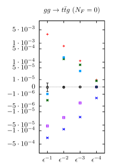
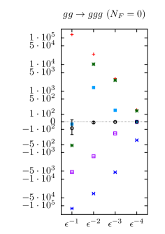
Figure 1: Illustration of the pole cancellation for the processes $gg\to t\bar{t}g$ (left panel) and $gg\to ggg$ (right panel) at a fixed phase space point for the underlying Born process. For each order in the dimensional regulator $\varepsilon$ the size of the individual contributions (see text) is plotted, as well as their sum, which is compatible with zero within the statistical errors of the Monte Carlo integration over the phase space of unresolved particles.

As a demonstration, that this procedure indeed works, let us take the example processes $gg\to t\bar{t}g$ and $gg\to ggg$ without massless quarks at NNLO. We make use of the fact that the new phase space construction allows us to keep the Born phase space configuration fixed while integrating over the unresolved phase space of all double unresolved configurations, i.e. up to two additional unresolved partons. Fig. 1 shows the cancellation of the $\varepsilon^{-4}$ to $\varepsilon^{-1}$ poles for a fixed Born phase space point. We plot the size of each contribution to $\hat{\sigma}_{\text{DU}}$ and their sum. The sum is compatible with zero within the statistical errors of the Monte Carlo integration, indicated by the error bars. The vertical axis is rescaled using $\sinh$ to show both positive and negative contributions at different orders of magnitude. The values themselves have no physical meaning but only demonstrate the pole cancellation. This shows that the subtraction scheme presented here works also for involved massive and massless QCD final states.

5 Conclusions

In this article we have discussed recent developments in the sector-improved residue subtraction scheme. We have developed a new phase space construction which minimizes the number of subtraction kinematics to reduce the probability of misbinning. Moreover, the scheme allows to easily fix a Born phase space point while integrating over the unresolved part of the phase space. This can be used for a pointwise check of pole cancellation. We also rederived the ’t Hooft-Veltman corrections which allow for a four-dimensional treatment of all resolved momenta and polarisations. Here, we made extensive use of the measurement functions to derive and calculate the corrections. As an illustration, we finally considered two involved processes, $gg\to t\bar{t}g$ and $gg\to ggg$, at NNLO and showed pole cancellation for a fixed Born configuration.

References

- [1] T. Kinoshita, Mass singularities of Feynman amplitudes, J. Math. Phys. 3 (1962) 650–677
- [2] T. D. Lee and M. Nauenberg, Degenerate Systems and Mass Singularities, Phys. Rev. 133 (1964) B1549–B1562
- [3] S. Catani and M. H. Seymour, A General algorithm for calculating jet cross-sections in NLO QCD, Nucl. Phys. B485 (1997) 291–419, [hep-ph/9605323], [Erratum: Nucl. Phys. B510 (1998) 503]
- [4] S. Catani and M. H. Seymour, The Dipole formalism for the calculation of QCD jet cross-sections at next-to-leading order, Phys. Lett. B378 (1996) 287–301, [hep-ph/9602277]
- [5] S. Frixione, Z. Kunszt and A. Signer, Three jet cross-sections to next-to-leading order, Nucl. Phys. B467 (1996) 399–442, [hep-ph/9512328]
- [6] R. Frederix, S. Frixione, F. Maltoni and T. Stelzer, Automation of next-to-leading order computations in QCD: The FKS subtraction, JHEP 10 (2009) 003, [0908.4272]
- [7] Z. Nagy and D. E. Soper, General subtraction method for numerical calculation of one loop QCD matrix elements, JHEP 09 (2003) 055, [hep-ph/0308127]
- [8] G. Bevilacqua, M. Czakon, M. Kubocz and M. Worek, Complete Nagy-Soper subtraction for next-to-leading order calculations in QCD, JHEP 10 (2013) 204, [1308.5605]
- [9] M. Czakon, H. B. Hartanto, M. Kraus and M. Worek, Matching the Nagy-Soper parton shower at next-to-leading order, JHEP 06 (2015) 033, [1502.00925]
- [10] A. Gehrmann-De Ridder, T. Gehrmann and E. W. N. Glover, Antenna subtraction at NNLO, JHEP 09 (2005) 056, [hep-ph/0505111]
- [11] J. Currie, E. W. N. Glover and S. Wells, Infrared Structure at NNLO Using Antenna Subtraction, JHEP 04 (2013) 066, [1301.4693]
- [12] A. Gehrmann-De Ridder, T. Gehrmann, E. W. N. Glover and G. Heinrich, Infrared structure of at NNLO, JHEP 11 (2007) 058, [0710.0346]
- [13] A. Gehrmann-De Ridder, T. Gehrmann and E. W. N. Glover, Infrared structure of at NNLO, Nucl. Phys. B691 (2004) 195–222, [hep-ph/0403057]
- [14] A. Gehrmann-De Ridder, T. Gehrmann and E. W. N. Glover, Quark-gluon antenna functions from neutralino decay, Phys. Lett. B612 (2005) 36–48, [hep-ph/0501291]
- [15] A. Gehrmann-De Ridder, T. Gehrmann and E. W. N. Glover, Gluon-gluon antenna functions from Higgs boson decay, Phys. Lett. B612 (2005) 49–60, [hep-ph/0502110]
- [16] A. Gehrmann-De Ridder, T. Gehrmann, E. W. N. Glover and G. Heinrich, Second-order QCD corrections to the thrust distribution, Phys. Rev. Lett. 99 (2007) 132002, [0707.1285]
- [17] A. Gehrmann-De Ridder, T. Gehrmann, E. W. N. Glover and G. Heinrich, NNLO corrections to event shapes in annihilation, JHEP 12 (2007) 094, [0711.4711]
- [18] A. Gehrmann-De Ridder, T. Gehrmann, E. W. N. Glover and G. Heinrich, Jet rates in electron-positron annihilation at in QCD, Phys. Rev. Lett. 100 (2008) 172001, [0802.0813]
- [19] A. Gehrmann-De Ridder, T. Gehrmann, E. W. N. Glover and G. Heinrich, NNLO moments of event shapes in annihilation, JHEP 05 (2009) 106, [0903.4658]
- [20] S. Weinzierl, NNLO corrections to 2-jet observables in electron-positron annihilation, Phys. Rev. D74 (2006) 014020, [hep-ph/0606008]
- [21] S. Weinzierl, The Forward-backward asymmetry at NNLO revisited, Phys. Lett. B644 (2007) 331–335, [hep-ph/0609021]
- [22] S. Weinzierl, NNLO corrections to 3-jet observables in electron-positron annihilation, Phys. Rev. Lett. 101 (2008) 162001, [0807.3241]
- [23] S. Weinzierl, The infrared structure of jets at NNLO reloaded, JHEP 07 (2009) 009, [0904.1145]
- [24] J. Currie, A. Gehrmann-De Ridder, E. W. N. Glover and J. Pires, NNLO QCD corrections to jet production at hadron colliders from gluon scattering, JHEP 01 (2014) 110, [1310.3993]
- [25] J. Currie, T. Gehrmann and J. Niehues, Precise QCD predictions for the production of dijet final states in deep inelastic scattering, Phys. Rev. Lett. 117 (2016) 042001, [1606.03991]
- [26] J. Currie, T. Gehrmann, A. Huss and J. Niehues, NNLO QCD corrections to jet production in deep inelastic scattering, JHEP 07 (2017) 018, [1703.05977]
- [27] J. Currie, A. Gehrmann-De Ridder, T. Gehrmann, E. W. N. Glover, A. Huss and J. Pires, Precise predictions for dijet production at the LHC, Phys. Rev. Lett. 119 (2017) 152001, [1705.10271]
- [28] D. Britzger, J. Currie, T. Gehrmann, A. Huss, J. Niehues and R. Zlebcik, Dijet production in diffractive deep-inelastic scattering in next-to-next-to-leading order QCD, Eur. Phys. J. C78 (2018) 538, [1804.05663]
- [29] J. Currie, A. Gehrmann-De Ridder, T. Gehrmann, N. Glover, A. Huss and J. Pires, Jet cross sections at the LHC with NNLOJET, in 14th DESY Workshop on Elementary Particle Physics: Loops and Legs in Quantum Field Theory 2018 (LL2018) St Goar, Germany, April 29-May 4, 2018, 2018. 1807.06057
- [30] W. Bernreuther, C. Bogner and O. Dekkers, The real radiation antenna function for at NNLO QCD, JHEP 06 (2011) 032, [1105.0530]
- [31] W. Bernreuther, C. Bogner and O. Dekkers, The real radiation antenna functions for at NNLO QCD, JHEP 10 (2013) 161, [1309.6887]
- [32] L. Chen, O. Dekkers, D. Heisler, W. Bernreuther and Z.-G. Si, Top-quark pair production at next-to-next-to-leading order QCD in electron positron collisions, JHEP 12 (2016) 098, [1610.07897]
- [33] W. Bernreuther, L. Chen, O. Dekkers, T. Gehrmann and D. Heisler, The forward-backward asymmetry for massive bottom quarks at the peak at next-to-next-to-leading order QCD, JHEP 01 (2017) 053, [1611.07942]
- [34] W. Bernreuther, L. Chen and Z.-G. Si, Differential decay rates of CP-even and CP-odd Higgs bosons to top and bottom quarks at NNLO QCD, JHEP 07 (2018) 159, [1805.06658]
- [35] G. Abelof and A. Gehrmann-De Ridder, Antenna subtraction for the production of heavy particles at hadron colliders, JHEP 04 (2011) 063, [1102.2443]
- [36] G. Abelof and A. Gehrmann-De Ridder, Double real radiation corrections to production at the LHC: the all-fermion processes, JHEP 04 (2012) 076, [1112.4736]
- [37] G. Abelof and A. Gehrmann-De Ridder, Double real radiation corrections to production at the LHC: the channel, JHEP 11 (2012) 074, [1207.6546]
- [38] G. Abelof, O. Dekkers and A. Gehrmann-De Ridder, Antenna subtraction with massive fermions at NNLO: Double real initial-final configurations, JHEP 12 (2012) 107, [1210.5059]
- [39] G. Abelof, A. Gehrmann-De Ridder, P. Maierhöfer and S. Pozzorini, NNLO QCD subtraction for top-antitop production in the channel, JHEP 08 (2014) 035, [1404.6493]
- [40] G. Abelof and A. Gehrmann-De Ridder, Light fermionic NNLO QCD corrections to top-antitop production in the quark-antiquark channel, JHEP 12 (2014) 076, [1409.3148]
- [41] G. Abelof, A. Gehrmann-De Ridder and I. Majer, Top quark pair production at NNLO in the quark-antiquark channel, JHEP 12 (2015) 074, [1506.04037]
- [42] X. Chen, T. Gehrmann, E. W. N. Glover and M. Jaquier, Precise QCD predictions for the production of Higgs + jet final states, Phys. Lett. B740 (2015) 147–150, [1408.5325]
- [43] X. Chen, J. Cruz-Martinez, T. Gehrmann, E. W. N. Glover and M. Jaquier, NNLO QCD corrections to Higgs boson production at large transverse momentum, JHEP 10 (2016) 066, [1607.08817]
- [44] X. Chen, T. Gehrmann, E. W. N. Glover, A. Huss, Y. Li, D. Neill et al., Precise QCD Description of the Higgs Boson Transverse Momentum Spectrum, 1805.00736
- [45] J. Cruz-Martinez, T. Gehrmann, E. W. N. Glover and A. Huss, Second-order QCD effects in Higgs boson production through vector boson fusion, Phys. Lett. B781 (2018) 672–677, [1802.02445]
- [46] J. Cruz-Martinez, E. W. N. Glover, T. Gehrmann and A. Huss, NNLO corrections to VBF Higgs boson production, 1807.07908
- [47] A. Gehrmann-De Ridder, T. Gehrmann, E. W. N. Glover, A. Huss and D. M. Walker, Next-to-Next-to-Leading-Order QCD Corrections to the Transverse Momentum Distribution of Weak Gauge Bosons, Phys. Rev. Lett. 120 (2018) 122001, [1712.07543]
- [48] J. Niehues and D. M. Walker, NNLO QCD Corrections to Jet Production in Charged Current Deep Inelastic Scattering, 1807.02529
- [49] A. Gehrmann-De Ridder, T. Gehrmann, N. Glover, A. Huss and D. Walker, NNLO QCD Corrections to W+jet Production in NNLOJET, in 14th DESY Workshop on Elementary Particle Physics: Loops and Legs in Quantum Field Theory 2018 (LL2018) St Goar, Germany, April 29-May 4, 2018, 2018. 1807.09113
- [50] G. Somogyi, Z. Trocsanyi and V. Del Duca, Matching of singly- and doubly-unresolved limits of tree-level QCD squared matrix elements, JHEP 06 (2005) 024, [hep-ph/0502226]
- [51] G. Somogyi, Z. Trocsanyi and V. Del Duca, A Subtraction scheme for computing QCD jet cross sections at NNLO: Regularization of doubly-real emissions, JHEP 01 (2007) 070, [hep-ph/0609042]
- [52] G. Somogyi and Z. Trocsanyi, A Subtraction scheme for computing QCD jet cross sections at NNLO: Regularization of real-virtual emission, JHEP 01 (2007) 052, [hep-ph/0609043]
- [53] U. Aglietti, V. Del Duca, C. Duhr, G. Somogyi and Z. Trocsanyi, Analytic integration of real-virtual counterterms in NNLO jet cross sections. I., JHEP 09 (2008) 107, [0807.0514]
- [54] V. Del Duca, G. Somogyi and Z. Trocsanyi, Integration of collinear-type doubly unresolved counterterms in NNLO jet cross sections, JHEP 06 (2013) 079, [1301.3504]
- [55] A. Kardos, G. Somogyi and Z. Tulipant, NNLO QCD calculations with CoLoRFulNNLO, PoS RADCOR2017 (2017) 018
- [56] A. Kardos, G. Bevilacqua, G. Somogyi, Z. Trocsanyi and Z. Tulipant, CoLoRFulNNLO for LHC processes, in 14th DESY Workshop on Elementary Particle Physics: Loops and Legs in Quantum Field Theory 2018 (LL2018) St Goar, Germany, April 29-May 4, 2018, 2018. 1807.04976
- [57] V. Del Duca, C. Duhr, G. Somogyi, F. Tramontano and Z. Trocsanyi, Higgs boson decay into b-quarks at NNLO accuracy, JHEP 04 (2015) 036, [1501.07226]
- [58] V. Del Duca, C. Duhr, A. Kardos, G. Somogyi and Z. Trocsanyi, Three-Jet Production in Electron-Positron Collisions at Next-to-Next-to-Leading Order Accuracy, Phys. Rev. Lett. 117 (2016) 152004, [1603.08927]
- [59] V. Del Duca, C. Duhr, A. Kardos, G. Somogyi, Z. Szor, Z. Trocsanyi et al., Jet production in the CoLoRFulNNLO method: event shapes in electron-positron collisions, Phys. Rev. D94 (2016) 074019, [1606.03453]
- [60] A. Kardos, S. Kluth, G. Somogyi, Z. Tulipant and A. Verbytskyi, Precise determination of from a global fit of energy-energy correlation to NNLO+NNLL predictions, Eur. Phys. J. C78 (2018) 498, [1804.09146]
- [61] S. Catani and M. Grazzini, An NNLO subtraction formalism in hadron collisions and its application to Higgs boson production at the LHC, Phys. Rev. Lett. 98 (2007) 222002, [hep-ph/0703012]
- [62] S. Catani, L. Cieri, G. Ferrera, D. de Florian and M. Grazzini, Vector boson production at hadron colliders: a fully exclusive QCD calculation at NNLO, Phys. Rev. Lett. 103 (2009) 082001, [0903.2120]
- [63] G. Ferrera, M. Grazzini and F. Tramontano, Associated WH production at hadron colliders: a fully exclusive QCD calculation at NNLO, Phys. Rev. Lett. 107 (2011) 152003, [1107.1164]
- [64] S. Catani, L. Cieri, D. de Florian, G. Ferrera and M. Grazzini, Diphoton production at hadron colliders: a fully-differential QCD calculation at NNLO, Phys. Rev. Lett. 108 (2012) 072001, [1110.2375], [Erratum: Phys. Rev. Lett. 117, (2016) 089901]
- [65] T. Gehrmann, M. Grazzini, S. Kallweit, P. Maierhöfer, A. von Manteuffel, S. Pozzorini et al., Production at Hadron Colliders in Next to Next to Leading Order QCD, Phys. Rev. Lett. 113 (2014) 212001, [1408.5243]
- [66] F. Cascioli, T. Gehrmann, M. Grazzini, S. Kallweit, P. Maierhöfer, A. von Manteuffel et al., ZZ production at hadron colliders in NNLO QCD, Phys. Lett. B735 (2014) 311–313, [1405.2219]
- [67] M. Grazzini, S. Kallweit, D. Rathlev and A. Torre, production at hadron colliders in NNLO QCD, Phys. Lett. B731 (2014) 204–207, [1309.7000]
- [68] M. Grazzini, S. Kallweit and D. Rathlev, and production at the LHC in NNLO QCD, JHEP 07 (2015) 085, [1504.01330]
- [69] R. Bonciani, S. Catani, M. Grazzini, H. Sargsyan and A. Torre, The subtraction method for top quark production at hadron colliders, Eur. Phys. J. C75 (2015) 581, [1508.03585]
- [70] M. Grazzini, S. Kallweit and D. Rathlev, ZZ production at the LHC: fiducial cross sections and distributions in NNLO QCD, Phys. Lett. B750 (2015) 407–410, [1507.06257]
- [71] M. Grazzini, S. Kallweit, S. Pozzorini, D. Rathlev and M. Wiesemann, production at the LHC: fiducial cross sections and distributions in NNLO QCD, JHEP 08 (2016) 140, [1605.02716]
- [72] D. de Florian, M. Grazzini, C. Hanga, S. Kallweit, J. M. Lindert, P. Maierhöfer et al., Differential Higgs Boson Pair Production at Next-to-Next-to-Leading Order in QCD, JHEP 09 (2016) 151, [1606.09519]
- [73] M. Grazzini, S. Kallweit, D. Rathlev and M. Wiesemann, production at the LHC: fiducial cross sections and distributions in NNLO QCD, JHEP 05 (2017) 139, [1703.09065]
- [74] M. Grazzini, S. Kallweit and M. Wiesemann, Fully differential NNLO computations with MATRIX, Eur. Phys. J. C78 (2018) 537, [1711.06631]
- [75] M. Grazzini, G. Heinrich, S. Jones, S. Kallweit, M. Kerner, J. M. Lindert et al., Higgs boson pair production at NNLO with top quark mass effects, JHEP 05 (2018) 059, [1803.02463]
- [76] J. Gaunt, M. Stahlhofen, F. J. Tackmann and J. R. Walsh, N-jettiness Subtractions for NNLO QCD Calculations, JHEP 09 (2015) 058, [1505.04794]
- [77] R. Boughezal, C. Focke, W. Giele, X. Liu and F. Petriello, Higgs boson production in association with a jet at NNLO using jettiness subtraction, Phys. Lett. B748 (2015) 5–8, [1505.03893]
- [78] R. Boughezal, J. M. Campbell, R. K. Ellis, C. Focke, W. T. Giele, X. Liu et al., Z-boson production in association with a jet at next-to-next-to-leading order in perturbative QCD, Phys. Rev. Lett. 116 (2016) 152001, [1512.01291]
- [79] R. Boughezal, J. M. Campbell, R. K. Ellis, C. Focke, W. Giele, X. Liu et al., Color singlet production at NNLO in MCFM, Eur. Phys. J. C77 (2017) 7, [1605.08011]
- [80] J. M. Campbell, R. K. Ellis and C. Williams, Associated production of a Higgs boson at NNLO, JHEP 06 (2016) 179, [1601.00658]
- [81] J. M. Campbell, R. K. Ellis, Y. Li and C. Williams, Predictions for diphoton production at the LHC through NNLO in QCD, JHEP 07 (2016) 148, [1603.02663]
- [82] J. M. Campbell, R. K. Ellis and C. Williams, Direct Photon Production at Next-to-Next-to-Leading Order, Phys. Rev. Lett. 118 (2017) 222001, [1612.04333]
- [83] I. Moult, L. Rothen, I. W. Stewart, F. J. Tackmann and H. X. Zhu, Subleading Power Corrections for N-Jettiness Subtractions, Phys. Rev. D95 (2017) 074023, [1612.00450]
- [84] I. Moult, L. Rothen, I. W. Stewart, F. J. Tackmann and H. X. Zhu, N -jettiness subtractions for at subleading power, Phys. Rev. D97 (2018) 014013, [1710.03227]
- [85] M. A. Ebert, I. Moult, I. W. Stewart, F. J. Tackmann, G. Vita and H. X. Zhu, Power Corrections for N-Jettiness Subtractions at , 1807.10764
- [86] M. Czakon, A novel subtraction scheme for double-real radiation at NNLO, Phys. Lett. B693 (2010) 259–268, [1005.0274]
- [87] M. Czakon, Double-real radiation in hadronic top quark pair production as a proof of a certain concept, Nucl. Phys. B849 (2011) 250–295, [1101.0642]
- [88] M. Czakon and D. Heymes, Four-dimensional formulation of the sector-improved residue subtraction scheme, Nucl. Phys. B890 (2014) 152–227, [1408.2500]
- [89] P. Bärnreuther, M. Czakon and A. Mitov, Percent Level Precision Physics at the Tevatron: First Genuine NNLO QCD Corrections to , Phys. Rev. Lett. 109 (2012) 132001, [1204.5201]
- [90] M. Czakon and A. Mitov, NNLO corrections to top-pair production at hadron colliders: the all-fermionic scattering channels, JHEP 12 (2012) 054, [1207.0236]
- [91] M. Czakon and A. Mitov, NNLO corrections to top pair production at hadron colliders: the quark-gluon reaction, JHEP 01 (2013) 080, [1210.6832]
- [92] M. Czakon, P. Fiedler and A. Mitov, Total Top-Quark Pair-Production Cross Section at Hadron Colliders Through , Phys. Rev. Lett. 110 (2013) 252004, [1303.6254]
- [93] M. Czakon, P. Fiedler and A. Mitov, Resolving the Tevatron Top Quark Forward-Backward Asymmetry Puzzle: Fully Differential Next-to-Next-to-Leading-Order Calculation, Phys. Rev. Lett. 115 (2015) 052001, [1411.3007]
- [94] M. Czakon, D. Heymes and A. Mitov, High-precision differential predictions for top-quark pairs at the LHC, Phys. Rev. Lett. 116 (2016) 082003, [1511.00549]
- [95] M. Czakon, P. Fiedler, D. Heymes and A. Mitov, NNLO QCD predictions for fully-differential top-quark pair production at the Tevatron, JHEP 05 (2016) 034, [1601.05375]
- [96] M. Czakon, D. Heymes and A. Mitov, fastNLO tables for NNLO top-quark pair differential distributions, 1704.08551
- [97] R. Boughezal, K. Melnikov and F. Petriello, A subtraction scheme for NNLO computations, Phys. Rev. D85 (2012) 034025, [1111.7041]
- [98] R. Boughezal, F. Caola, K. Melnikov, F. Petriello and M. Schulze, Higgs boson production in association with a jet at next-to-next-to-leading order in perturbative QCD, JHEP 06 (2013) 072, [1302.6216]
- [99] R. Boughezal, F. Caola, K. Melnikov, F. Petriello and M. Schulze, Higgs boson production in association with a jet at next-to-next-to-leading order, Phys. Rev. Lett. 115 (2015) 082003, [1504.07922]
- [100] F. Caola, K. Melnikov and R. Röntsch, Nested soft-collinear subtractions in NNLO QCD computations, Eur. Phys. J. C77 (2017) 248, [1702.01352]
- [101] F. Caola, G. Luisoni, K. Melnikov and R. Röntsch, NNLO QCD corrections to associated production and decay, Phys. Rev. D97 (2018) 074022, [1712.06954]
- [102] R. Röntsch, Nested soft-collinear subtractions for NNLO calculations, PoS RADCOR2017 (2018) 031
- [103] M. Brucherseifer, F. Caola and K. Melnikov, corrections to fully-differential top quark decays, JHEP 04 (2013) 059, [1301.7133]
- [104] M. Brucherseifer, F. Caola and K. Melnikov, On the corrections to inclusive decays, Phys. Lett. B721 (2013) 107–110, [1302.0444]
- [105] M. Brucherseifer, F. Caola and K. Melnikov, On the NNLO QCD corrections to single-top production at the LHC, Phys. Lett. B736 (2014) 58–63, [1404.7116]
- [106] F. Caola, A. Czarnecki, Y. Liang, K. Melnikov and R. Szafron, Muon decay spin asymmetry, Phys. Rev. D90 (2014) 053004, [1403.3386]
- [107] M. Cacciari, F. A. Dreyer, A. Karlberg, G. P. Salam and G. Zanderighi, Fully Differential Vector-Boson-Fusion Higgs Production at Next-to-Next-to-Leading Order, Phys. Rev. Lett. 115 (2015) 082002, [1506.02660], [Erratum: Phys. Rev. Lett. 120 (2018) 139901]
- [108] J. Currie, T. Gehrmann, E. W. N. Glover, A. Huss, J. Niehues and A. Vogt, N3LO corrections to jet production in deep inelastic scattering using the Projection-to-Born method, JHEP 05 (2018) 209, [1803.09973]
- [109] L. Magnea, E. Maina, P. Torrielli and S. Uccirati, Factorization and subtraction, PoS RADCOR2017 (2018) 043, [1801.06462]
- [110] L. Magnea, E. Maina, P. Torrielli and S. Uccirati, Towards analytic local sector subtraction at NNLO, PoS RADCOR2017 (2018) 035, [1801.06458]
- [111] L. Magnea, E. Maina, G. Pelliccioli, C. Signorile-Signorile, P. Torrielli and S. Uccirati, Local Analytic Sector Subtraction at NNLO, 1806.09570
- [112] F. Herzog, Geometric IR subtraction for final state real radiation, JHEP 08 (2018) 006, [1804.07949]
- [113] T. Binoth and G. Heinrich, An automatized algorithm to compute infrared divergent multiloop integrals, Nucl. Phys. B585 (2000) 741–759, [hep-ph/0004013]
- [114] C. Anastasiou, K. Melnikov and F. Petriello, A new method for real radiation at NNLO, Phys. Rev. D69 (2004) 076010, [hep-ph/0311311]
- [115] T. Binoth and G. Heinrich, Numerical evaluation of phase space integrals by sector decomposition, Nucl. Phys. B693 (2004) 134–148, [hep-ph/0402265]
- [116] S. M. Aybat, L. J. Dixon and G. F. Sterman, The Two-loop soft anomalous dimension matrix and resummation at next-to-next-to leading pole, Phys. Rev. D74 (2006) 074004, [hep-ph/0607309]
- [117] T. Becher and M. Neubert, Infrared singularities of QCD amplitudes with massive partons, Phys. Rev. D79 (2009) 125004, [0904.1021], [Erratum: Phys. Rev. D80 (2009) 109901]
- [118] M. Czakon, A. Mitov and G. F. Sterman, Threshold Resummation for Top-Pair Hadroproduction to Next-to-Next-to-Leading Log, Phys. Rev. D80 (2009) 074017, [0907.1790]
- [119] A. Mitov, G. F. Sterman and I. Sung, The Massive Soft Anomalous Dimension Matrix at Two Loops, Phys. Rev. D79 (2009) 094015, [0903.3241]
- [120] A. Ferroglia, M. Neubert, B. D. Pecjak and L. L. Yang, Two-loop divergences of massive scattering amplitudes in non-abelian gauge theories, JHEP 11 (2009) 062, [0908.3676]
- [121] A. Mitov, G. F. Sterman and I. Sung, Computation of the Soft Anomalous Dimension Matrix in Coordinate Space, Phys. Rev. D82 (2010) 034020, [1005.4646]
- [122] T. Becher and M. Neubert, Infrared singularities of scattering amplitudes in perturbative QCD, Phys. Rev. Lett. 102 (2009) 162001, [0901.0722], [Erratum: Phys. Rev. Lett. 111 (2013) 199905]
- [123] S. Catani and M. Grazzini, Infrared factorization of tree level QCD amplitudes at the next-to-next-to-leading order and beyond, Nucl. Phys. B570 (2000) 287–325, [hep-ph/9908523]
- [124] J. M. Campbell and E. W. N. Glover, Double unresolved approximations to multiparton scattering amplitudes, Nucl. Phys. B527 (1998) 264–288, [hep-ph/9710255]
- [125] S. Catani and M. Grazzini, Collinear factorization and splitting functions for next-to-next-to-leading order QCD calculations, Phys. Lett. B446 (1999) 143–152, [hep-ph/9810389]
- [126] Z. Bern, L. J. Dixon, D. C. Dunbar and D. A. Kosower, One loop n point gauge theory amplitudes, unitarity and collinear limits, Nucl. Phys. B425 (1994) 217–260, [hep-ph/9403226]
- [127] Z. Bern, V. Del Duca and C. R. Schmidt, The Infrared behavior of one loop gluon amplitudes at next-to-next-to-leading order, Phys. Lett. B445 (1998) 168–177, [hep-ph/9810409]
- [128] D. A. Kosower, All order collinear behavior in gauge theories, Nucl. Phys. B552 (1999) 319–336, [hep-ph/9901201]
- [129] D. A. Kosower and P. Uwer, One loop splitting amplitudes in gauge theory, Nucl. Phys. B563 (1999) 477–505, [hep-ph/9903515]
- [130] S. Catani and M. Grazzini, The soft gluon current at one loop order, Nucl. Phys. B591 (2000) 435–454, [hep-ph/0007142]
- [131] I. Bierenbaum, M. Czakon and A. Mitov, The singular behavior of one-loop massive QCD amplitudes with one external soft gluon, Nucl. Phys. B856 (2012) 228–246, [1107.4384]
- [132] M. L. Czakon and A. Mitov, A simplified expression for the one-loop soft-gluon current with massive fermions, 1804.02069
- [133] G. ’t Hooft and M. J. G. Veltman, Regularization and Renormalization of Gauge Fields, Nucl. Phys. B44 (1972) 189–213
- [134] J. F. Ashmore, A Method of Gauge Invariant Regularization, Lett. Nuovo Cim. 4 (1972) 289–290
- [135] G. M. Cicuta and E. Montaldi, Analytic renormalization via continuous space dimension, Lett. Nuovo Cim. 4 (1972) 329–332
- [136] C. G. Bollini and J. J. Giambiagi, Dimensional Renormalization: The Number of Dimensions as a Regularizing Parameter, Nuovo Cim. B12 (1972) 20–26
- [137] W. J. Marciano and A. Sirlin, Dimensional Regularization of Infrared Divergences, Nucl. Phys. B88 (1975) 86–98
- [138] S. Frixione and B. R. Webber, Matching NLO QCD computations and parton shower simulations, JHEP 06 (2002) 029, [hep-ph/0204244]
- [139] S. Frixione, P. Nason and C. Oleari, Matching NLO QCD computations with Parton Shower simulations: the POWHEG method, JHEP 11 (2007) 070, [0709.2092]