Diffusive Nambu-Goldstone modes in quantum time-crystals: Supplemental material

I Schwinger-Keldysh formalism in an open quantum sytem

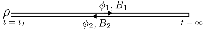
Figure 1: Closed time contour in the Schwinger-Keldysh formalism.

We here derive the path integral formula for an open quantum system used in the main text. We consider a quantum system coupled with an environment. The path integral formula for an open quantum system is obtained by integrating the environment out. In general, the action of the total system has three parts:

$$\begin{split}S_{\text{tot}}[\varphi,B]=S_{\text{sys}}[\varphi]+S_{\text{env}}[B]+S_{\text{int}}[\varphi,B],\end{split}$$ (1)

where $S_{\text{sys}}[\varphi]$, $S_{\text{env}}[B]$, and $S_{\text{int}}[B,\varphi]$ are the actions of the system, environment, and interaction, respectively. $\varphi$ and $B$ are the degrees of freedom of the system and environment. We assume that the initial density matrix at $t=t_{I}$ is the direct product of those of the system and environment: $\hat{\rho}=\hat{\rho}_{\text{sys}}\otimes\hat{\rho}_{\text{env}}$. We consider the following path integral whose path is shown in Fig. 1:

$$\begin{split}Z&=\int\mathcal{D}\varphi_{1}\mathcal{D}\varphi_{2}\mathcal{D}B_{1}\mathcal{D}B_{2}\rho_{\text{sys}}(\varphi_{I1},\varphi_{I2})\rho_{\text{env}}(B_{I1},B_{I2})\\ &\quad\times e^{iS_{\text{tot}}[\varphi_{1},B_{1}]-iS_{\text{tot}}[\varphi_{2},B_{2}]},\end{split}$$ (2)

where the indices, $1$ and $2$, represent the label of the forward and backward paths in Fig. 1, and we introduced the matrix elements of the density operators $\rho_{\text{sys}}(\varphi_{I1},\varphi_{I2}):=\langle\varphi_{1}(t_{I})|\hat{\rho}_{\text{sys}}|\varphi_{2}(t_{I})\rangle$ and $\rho_{\text{env}}(B_{I1},B_{I2}):=\langle B_{1}(t_{I})|\hat{\rho}_{\text{env}}|B_{2}(t_{I})\rangle$. The direct product of the density operators enables us to formally integrate the environment out. Then, introducing

$$\begin{split}e^{i\Gamma[\varphi_{1},\varphi_{2}]}&:=\int\mathcal{D}B_{1}\mathcal{D}B_{2}\rho_{\text{env}}(B_{I1},B_{I2})\\ &\quad\times e^{iS_{\text{env}}[B_{1}]-iS_{\text{env}}[B_{2}]+iS_{\text{int}}[\varphi_{1},B_{1}]-iS_{\text{int}}[\varphi_{2},B_{1}]},\end{split}$$ (3)

we can express the path integral of the system as

$$\begin{split}Z=\int\mathcal{D}\varphi_{1}\mathcal{D}\varphi_{2}\rho_{\text{sys}}(\varphi_{I1},\varphi_{I2})e^{iS_{\text{eff}}[\varphi_{1},\varphi_{2}]},\end{split}$$ (4)

where we define

$$\begin{split}S_{\text{eff}}[\varphi_{1},\varphi_{2}]:=S_{\text{sys}}[\varphi_{1}]-S_{\text{sys}}[\varphi_{2}]+\Gamma[\varphi_{1},\varphi_{2}].\end{split}$$ (5)

An observable ${O}(\varphi_{1},\varphi_{2})$ of the system is evaluated as

$$\begin{split}&\langle{O}(\varphi_{1},\varphi_{2})\rangle\\ &\quad:=\frac{1}{Z}\int\mathcal{D}\varphi_{1}\mathcal{D}\varphi_{2}\rho_{\text{sys}}(\varphi_{I1},\varphi_{I2})e^{iS_{\text{eff}}[\varphi_{1},\varphi_{2}]}{O}(\varphi_{1},\varphi_{2}).\end{split}$$ (6)

When we take $t_{I}\to-\infty$, $\rho_{\text{sys}}(\varphi_{I1},\varphi_{I2})$ and ${O}(\varphi_{1},\varphi_{2})$ will be uncorrelated. Then, we can write the path integral as the form in Eq. (6) in the main text (by generalizing to complex fields).

The $R/A$ basis used in the main text is defined as $\varphi_{R}:=(\varphi_{1}+\varphi_{2})/2$ and $\varphi_{A}:=(\varphi_{1}-\varphi_{2})$. For example, the action of the $\lambda\varphi^{4}$ theory has the form:

$$\begin{split}S_{\text{sys}}[\varphi]=\int d^{4}x\Bigl{(}\frac{1}{2}(\partial_{t}\varphi)^{2}-\frac{1}{2}(\nabla\varphi)^{2}-\frac{\lambda}{2}\varphi^{4}\Bigr{)}.\end{split}$$ (7)

In the $R/A$ basis, $S_{\text{sys}}[\varphi_{1}]-S_{\text{sys}}[\varphi_{2}]$ is expressed as

$$\begin{split}&S_{\text{sys}}[\varphi_{1}]-S_{\text{sys}}[\varphi_{2}]\\ &=\int d^{4}x\Bigl{(}\varphi_{A}(-\partial_{t}^{2}\varphi_{R}+\nabla^{2}\varphi_{R}-2\lambda\varphi_{R}^{3})-\frac{\lambda}{2}\varphi_{R}\varphi_{A}^{3}\Bigr{)}\\ &\quad+\text{boundary term}.\end{split}$$ (8)

This corresponds to the action (13) in the main text with $\gamma=A=0$. The functional form of $\Gamma[\varphi_{1},\varphi_{2}]$ depends on the details of the environment. In our van der Pol model in the main text, we chose

$$\begin{split}\Gamma[\varphi_{1},\varphi_{2}]=\int d^{4}x\Bigl{[}\varphi_{A}\gamma(1-\kappa\varphi^{2}_{R})\partial_{t}\varphi_{R}+iA\varphi_{A}^{2}\Bigr{]}.\end{split}$$ (9)

II Noether current

Let us consider an action $S$ as a functional of complex scalar fields $\varPhi_{R}$ and $\varPhi_{A}$. Suppose that the action $S$ is invariant under an infinitesimal transformation $\varPhi_{R}\to\varPhi_{R}+\epsilon_{a}\delta_{A}^{a}\varPhi_{R}$, and $\varPhi_{A}\to\varPhi_{A}+\epsilon_{a}\delta_{A}^{a}\varPhi_{A}$, where $\epsilon_{a}$ is an infinitesimal small constant. For example, the time translation and $U(1)$ transformations are written as

$$\begin{split}\delta_{A}^{T}\varPhi_{R}&:=\partial_{t}\varPhi_{R},\qquad\delta_{A}^{T}\varPhi_{A}:=\partial_{t}\varPhi_{A},\end{split}$$ (10)

and

$$\begin{split}\delta_{A}^{Q}\varPhi_{R}&:=i\varPhi_{R},\qquad\delta_{A}^{Q}\varPhi_{A}:=i\varPhi_{A},\end{split}$$ (11)

respectively. For spacetime-dependent parameters $\epsilon_{a}(x)$, the action behaves as

$$\begin{split}S\to S-\int d^{4}x\bigl{(}\partial_{\mu}\epsilon_{a}(x)\bigr{)}j_{A}^{a\mu}(x),\end{split}$$ (12)

because the last term must vanish for constant $\epsilon_{a}$. Here, $j_{A}^{a\mu}$ is the so-called Noether current Weinberg (1995). For the $U(1)$ symmetry of the action (17) in the main text, the explicit form of $j_{A}^{Q0}(x)$ is given as

$$\begin{split}j_{A}^{Q0}&=i(\varPhi_{A}^{*}(\partial_{t}+i\mu)\varPhi_{R}-(\partial_{t}-i\mu)\varPhi_{A}^{*}\varPhi_{R})\\ &\quad+i(\varPhi_{R}^{*}(\partial_{t}+i\mu)\varPhi_{A}-(\partial_{t}-i\mu)\varPhi_{R}^{*}\varPhi_{A})\\ &\quad+i\gamma(1-\kappa|\varPhi_{R}|^{2})(\varPhi_{R}^{*}\varPhi_{A}-\varPhi_{A}^{*}\varPhi_{R})\\ &\quad+i\lambda(\varPhi_{R}\partial_{t}\varPhi_{R}^{*}-\partial_{t}\varPhi_{R}\varPhi_{R}^{*})(\varPhi_{R}^{*}\varPhi_{A}+\varPhi_{A}^{*}\varPhi_{R}).\end{split}$$ (13)

Similarly, the charge density of the time translation reads

$$\begin{split}j_{A}^{T0}&=-\partial_{t}\varPhi_{A}^{*}\partial_{t}\varPhi_{R}-\partial_{t}\varPhi_{R}^{*}\partial_{t}\varPhi_{A}+\varPhi_{A}^{*}\nabla^{2}\varPhi_{R}+\varPhi_{R}^{*}\nabla^{2}\varPhi_{A}\\ &\quad+(\mu^{2}\!-\!m^{2}\!+\!\lambda|\partial_{t}\varPhi_{R}|^{2})(\varPhi_{A}^{*}\varPhi_{R}+\varPhi_{R}^{*}\varPhi_{A})\!+\!iA|\varPhi_{A}|^{2}.\end{split}$$ (14)

We can introduce the $R$ transformation such that $\delta_{R}^{a}\varPhi_{A}:=\delta_{A}^{a}\varPhi_{R}$, and $\delta_{R}^{a}\varPhi_{R}:=\delta_{A}^{a}\varPhi_{A}/4$. Using this, we define the generalized Watanabe-Brauner matrix as $\rho^{ab}=-\langle\delta_{R}^{a}j_{A}^{b0}\rangle$. For the superfluid kink time-crystal (17) in the main text, $\rho^{ab}$ is written explicitly as

$$\langle\delta_{R}^{T}j_{A}^{0T}\rangle =(\mu^{2}-m^{2}+\lambda|\dot{\varPhi}_{0}|^{2})\partial_{t}|{\varPhi}_{0}|^{2}-\partial_{t}(\dot{\varPhi}_{0}^{*}\dot{\varPhi}_{0}),$$ (15)

$$\langle\delta_{R}^{Q}j_{A}^{T0}\rangle =0,$$ (16)

$$\langle\delta_{R}^{T}j_{A}^{Q0}\rangle =i\partial_{t}({\varPhi}_{0}^{*}\dot{\varPhi}_{0}-\dot{\varPhi}_{0}^{*}\varPhi_{0}+2i\mu{\varPhi}_{0}^{*}\varPhi_{0})$$

$$\quad-i\gamma\left(1-\kappa|\varPhi_{0}|^{2}\right)(\dot{\varPhi}_{0}^{*}\varPhi_{0}-\varPhi_{0}^{*}\dot{\varPhi}_{0})$$

$$\quad+\lambda i(\varPhi_{0}\dot{\varPhi}_{0}^{*}-\dot{\varPhi}_{0}\varPhi_{0}^{*})\partial_{t}|\varPhi_{0}|^{2},$$ (17)

$$\langle\delta_{R}^{Q}j_{A}^{Q0}\rangle =-2\gamma\left(1-\kappa|\varPhi_{0}|^{2}\right)|\varPhi_{0}|^{2}.$$ (18)

Similarly, for the van der Pol oscillator (13) in the main text, the explicit form of the charge density of the time translation and $\langle\delta^{T}_{R}j_{A}^{T0}\rangle$ are, respectively, written as

$$j_{A}^{T0} =-\partial_{t}\varphi_{A}\partial_{t}\varphi_{R}+\varphi_{A}\left(\nabla^{2}-2\lambda\varphi_{R}^{2}\right)\varphi_{R}$$

$$\quad-\frac{\lambda}{2}\varphi_{A}^{3}\varphi_{R}+iA(\varphi_{A})^{2},$$ (19)

$$\langle\delta^{T}_{R}j_{A}^{T0}\rangle =-\partial_{t}\Bigl{(}\frac{1}{2}\dot{\varphi}_{0}^{2}+\lambda\frac{1}{2}\varphi_{0}^{4}\Bigr{)}.$$ (20)

III Perturbative solutions

We here describe the method to compute the dispersion relations of the NG modes in quantum time-crystals. We would like to solve a second rank linear ordinary differential equation:

$$\begin{split}D(t,\partial_{t},\mathbf{p})\phi_{\mathbf{p}}(t)=0,\end{split}$$ (21)

where $\mathbf{p}$ is a parameter. In our situation, $\mathbf{p}$ is momentum. Suppose that $D(t,\partial_{t},\mathbf{p})$ has the time-translational symmetry: $D(t+T,\partial_{t},\mathbf{p})=D(t,\partial_{t},\mathbf{p})$, with the period $T$. Because the rank is two, there are two solutions $\phi_{1,\mathbf{p}}(t)$ and $\phi_{2,\mathbf{p}}(t)$. The translational symmetry implies that $\phi_{1,\mathbf{p}}(t+T)$ and $\phi_{2,\mathbf{p}}(t+T)$ can be expressed as a linear combination of $\phi_{1,\mathbf{p}}(t)$ and $\phi_{2,\mathbf{p}}(t)$:

$$\begin{split}\begin{pmatrix}\phi_{1,\mathbf{p}}(t+T)\\ \phi_{2,\mathbf{p}}(t+T)\end{pmatrix}=A\begin{pmatrix}\phi_{1,\mathbf{p}}(t)\\ \phi_{2,\mathbf{p}}(t)\end{pmatrix},\end{split}$$ (22)

with

$$\begin{split}A=\begin{pmatrix}c_{11}&c_{12}\\ c_{21}&c_{22}\end{pmatrix}.\end{split}$$ (23)

We note that $A$ generally depends on the parameter $p$. If the eigenvalues of $A$ are nondegenerate, we can diagonalize $A$, with bases $\tilde{\phi}_{a,p}(t)$, i.e., $\tilde{\phi}_{a,\mathbf{p}}(t+T)=\lambda_{a}\tilde{\phi}_{a,\mathbf{p}}(t)$, where $a=1,2$. In the following we drop the index $a$. Obviously, $\lambda$ describes a large time behavior. We can parametrize $\lambda$ as $\lambda=e^{-i\omega T}$. In general, $\omega$ is complex, whose imaginary part is negative if the system is stable. We can write $\tilde{\phi}_{p}(t)$ as

$$\begin{split}\tilde{\phi}_{\mathbf{p}}(t)=e^{-i\omega t}u_{\mathbf{p}}(t),\end{split}$$ (24)

where $u_{\mathbf{p}}(t+T)=u_{\mathbf{p}}(t)$. The equation (21) reads

$$\begin{split}D(t,\partial_{t}-i\omega,\mathbf{p})u_{\mathbf{p}}(t)=0.\end{split}$$ (25)

Let us try to perturbatively solve this equation. For this purpose, we decompose $D(t,\partial_{t}-i\omega,\mathbf{p})$ into $H_{0}=D(t,\partial_{t},\mathbf{0})$ and $V:=D(t,\partial_{t}-i\omega,\mathbf{p})-D(t,\partial_{t},0,\mathbf{0})$. Then, the equation is written as

$$\begin{split}(H_{0}+V(\omega,\mathbf{p}))u_{\mathbf{p}}(t)=0.\end{split}$$ (26)

Let $\Psi_{n}(t)$ be eigenfunctions with the eigenvalues $E_{n}$ of $H_{0}$ ($E_{0}=0$) with the periodic boundary condition $\Psi_{n}(t+T)=\Psi_{n}(t)$, i.e.,

$$\begin{split}H_{0}\Psi_{n}(t)=E_{n}\Psi_{n}(t).\end{split}$$ (27)

Since $H_{0}$ is generally not hermite, we also need to introduce $\eta_{n}$ such that

$$\begin{split}H^{{\dagger}}_{0}{\eta}_{n}(t)={E}_{n}{\eta}_{n}(t),\end{split}$$ (28)

with

$$\begin{split}\int_{0}^{T}dt\eta^{{\dagger}}_{n}(t)\Psi_{m}(t)=\delta_{n,m}.\end{split}$$ (29)

Using this basis, we expand $u_{\omega,\mathbf{p}}(t)$ as

$$\begin{split}u_{\omega,\mathbf{p}}(t)=\sum_{n=0}^{\infty}c_{n}(\omega,\mathbf{p})\Psi_{n}(t).\end{split}$$ (30)

The condition of $c_{n}$ for the zero mode is at $\omega=0$, $\mathbf{p}=\mathbf{0}$, $c_{0}(0,\mathbf{0})=1$ and $c_{n}(0,\mathbf{0})=0$. We have

$$\begin{split}(H_{0}+V(\omega,\mathbf{p}))u_{\omega,\mathbf{p}}(t)&=\\ \sum_{n=0}^{\infty}c_{n}(\omega,\mathbf{p})(E_{n}+V(\omega,\mathbf{p}))\Psi_{n}(t)&=0.\end{split}$$ (31)

Multiplying $\eta_{m}^{{\dagger}}(t)$ and integrating Eq. (31) with respect to $t$, we find

$$\begin{split}c_{m}(\omega,\mathbf{p})E_{m}+\sum_{n}V_{mn}(\omega,\mathbf{p})c_{n}(\omega,\mathbf{p})=0,\end{split}$$ (32)

where

$$\begin{split}V_{mn}(\omega,\mathbf{p}):=\int_{0}^{T}dt\eta_{m}^{{\dagger}}(t)V(\omega,\mathbf{p})\Psi_{n}(t).\end{split}$$ (33)

At the leading expansion of $\omega$ and $\mathbf{p}$, the solution of Eq. (26) is obtained from $V_{00}(\omega,\mathbf{p})=0$; it gives the relation between $\omega$ and $\mathbf{p}$.

IV Van der Pol oscillator

The dispersion relation of the NG mode is obtained from the solution of $[(\rho-\dot{g})\partial_{t}+g(-\partial_{t}^{2}+\nabla^{2})]\chi=:D_{R}^{-1}\chi=0$, with $g=\langle\delta_{A}^{T}\varphi_{R}\rangle^{2}=\dot{\varphi}_{0}^{2}$, and $\rho=-\langle\delta_{R}^{T}j^{T0}\rangle=\partial_{t}(\dot{\varphi}_{0}^{2}/2+\lambda\varphi_{0}^{4}/2)=\dot{\varphi}_{0}^{2}\gamma(1-\kappa\varphi_{0}^{2})$. Here we used the equation of motion of $\varphi_{0}$ (Eq. (14) in the main text). We introduce $G_{R}^{-1}$ such that $D_{R}^{-1}=\dot{\varphi}_{0}G_{R}^{-1}\dot{\varphi}_{0}$, where

$$\begin{split}&G^{-1}_{R}(t,\partial_{t},\nabla)=\\ &-\partial^{2}_{t}+\nabla^{2}+\gamma\left(1-\kappa\varphi_{0}^{2}\right)\partial_{t}-2\gamma\kappa\varphi_{0}\dot{\varphi}_{0}-6\lambda\varphi_{0}^{2}.\;\;\end{split}$$ (34)

We can consider the equation $G_{R}^{-1}\delta\phi=0$ instead of $D_{R}^{-1}\chi=0$. Obviously, both carry the same information. For the technical reason of numerics, it is easier to find the solution of $G_{R}^{-1}\delta\phi=0$, rather than that of $D_{R}^{-1}\chi=0$. Therefore, in the following, we solve $G_{R}^{-1}\delta\phi=0$ on the basis of the method described in Sec. III. We take $D(t,\partial_{t},\mathbf{p})=G_{R}^{-1}(t,\partial_{t},\mathbf{p})$, $H_{0}:=G_{R}^{-1}(t,\partial_{t},\mathbf{0})$, and $V(\omega,\mathbf{p}):=D(t,\partial_{t}-i\omega,\mathbf{p})-D(t,\partial_{t},\mathbf{0})$, where

$$H_{0}=-\partial^{2}_{t}+\gamma\left(1-\kappa\varphi_{0}^{2}\right)\partial_{t}-2\gamma\kappa\varphi_{0}\dot{\varphi}_{0}-6\lambda\varphi_{0}^{2}.$$ (35)

Then, we define $\Psi_{0}$, and $\eta_{0}$ as

$$H_{0}\Psi_{0} =0,$$ (36)

$$H_{0}^{\dagger}\eta_{0} =0,$$ (37)

with

$$H_{0}^{\dagger}=-\partial^{2}_{t}-\gamma\left(1-\kappa\varphi_{0}^{2}\right)\partial_{t}-6\lambda\varphi_{0}^{2}.$$ (38)

By construction, we find $\Psi_{0}=\dot{\varphi}_{0}$. We numerically solve Eq. (37) under the periodic boundary condition, and compute the left zero-eigenvector $\eta_{0}$. Then, by multiplying $\eta_{0}^{{\dagger}}$ to the left-hand-sides of $V\Psi_{0}$, we perturbatively obtain the potential $V_{00}$ as

$$\begin{split}V_{00}(\omega,\mathbf{p})&=\int_{0}^{T}dt\;\eta_{0}^{{\dagger}}V(\omega,\mathbf{p})\dot{\varphi}_{0}\\ &=\int_{0}^{T}dt\;{\psi}_{0}^{{\dagger}}(-i\omega(\rho-\dot{g})+g(\omega^{2}-\mathbf{p}^{2}))\end{split}$$ (39)

where ${\psi}_{0}^{{\dagger}}=\eta_{0}^{{\dagger}}/\dot{\varphi}_{0}$. The normalization condition turns out to be

$$\begin{split}1=\int_{0}^{T}dt\eta^{{\dagger}}_{0}\Psi_{0}=\int_{0}^{T}dt\psi^{{\dagger}}_{0}g.\end{split}$$ (40)

The on-shell condition is solved as $V_{00}(\omega,\mathbf{p})=0$, which is nothing but Eqs. (15), and (16) in the main text.

V Superfluid kink time-crystal

The time periodic solution of Eq. (18) in the main text, is not strictly periodic but rather quasi-periodic: $\varPhi_{0}(t+T)=e^{i\Omega T}\varPhi_{0}(t)$, with constant $\Omega$ and $T$, and the linearized equation of motion of fluctuations is also quasi-periodic. In order to apply our technique in which the periodicity of the linearized equation is assumed, we redefine the fields such that the expectation value of $\varPhi_{0}(t)$ is periodic, i.e., $\varPhi_{R}(x)\to e^{-i\Omega t}\varPhi_{R}(x)$, and $\varPhi_{A}(x)\to e^{-i\Omega t}\varPhi_{A}(x)$. Under the transformations, the time derivative transforms as $\partial_{t}\to\partial_{t}+i\Omega$, and the linearized equation of motion of fluctuations becomes periodic. We work in this basis in the following analysis.

As the same as before, the dispersion relation of the NG mode is obtained from the solution of $[(\rho^{ab}-\dot{g}^{ab})\partial_{t}+g^{ab}(-\partial_{t}^{2}+\nabla^{2})]\chi_{b}=[D_{R}^{-1}\chi]_{b}=0$, where $g^{ab}=2\mathrm{Re}\,\langle\delta_{A}^{a}\varPhi_{R}\rangle\langle\delta_{A}^{b}\varPhi_{R}^{*}\rangle$, with $\langle\delta_{A}^{T}\varPhi_{R}\rangle=\dot{\varPhi}_{0}$ and $\langle\delta_{A}^{Q}\varPhi_{R}\rangle=i\varPhi_{0}$. The explicit expression of $\rho^{ab}$ is shown in Eqs. (15)-(18). Since both of the time-translation and $U(1)$ symmetries are spontaneously broken, $D_{R}^{-1}$ is a two-by-two matrix. Because of the same reason as before, we introduce $G_{R}^{-1}(t,\partial_{t},\nabla)$ such that

$$\begin{split}D_{R}^{-1}=U^{T}G_{R}^{-1}(t,\partial_{t},\nabla)U,\end{split}$$ (41)

where

$$\begin{split}U=\begin{pmatrix}\mathrm{Re}\,\langle\delta_{A}^{T}\varPhi_{R}\rangle&\mathrm{Re}\,\langle\delta_{A}^{Q}\varPhi_{R}\rangle\\ \mathrm{Im}\,\langle\delta_{A}^{T}\varPhi_{R}\rangle&\mathrm{Im}\,\langle\delta_{A}^{Q}\varPhi_{R}\rangle\end{pmatrix}=\begin{pmatrix}\dot{\varphi}_{10}&-\varphi_{20}\\ \dot{\varphi}_{20}&\varphi_{10}\end{pmatrix},\end{split}$$ (42)

and

$$[G_{R}^{-1}]_{11}=$$

$$-\partial_{t}^{2}+\nabla^{2}+\gamma\left(1-\kappa_{1}\left(\varphi_{10}^{2}+\varphi_{20}^{2}\right)\right)\partial_{t}-2\gamma\kappa_{1}\varphi_{10}\dot{\varphi}_{10}$$

$$+\mu^{2}-m^{2}-\lambda\left({\dot{\varphi}_{10}^{2}+\dot{\varphi}_{20}^{2}}\right)-2\lambda\varphi_{10}\dot{\varphi}_{10}\partial_{t},$$ (43)

$$[G_{R}^{-1}]_{12}=2\mu\partial_{t}-2\lambda\varphi_{10}\dot{\varphi}_{20}\partial_{t}-2\gamma\kappa_{1}\dot{\varphi}_{10}\varphi_{20},$$ (44)

$$[G_{R}^{-1}]_{21}=-2\mu\partial_{t}-2\lambda\dot{\varphi}_{10}\varphi_{20}\partial_{t}-2\gamma\kappa_{1}\varphi_{10}\dot{\varphi}_{20},$$ (45)

$$[G_{R}^{-1}]_{22}=$$

$$-\partial_{t}^{2}+\nabla^{2}+\gamma\left(1-\kappa_{1}\left(\varphi_{10}^{2}+\varphi_{20}^{2}\right)\right)\partial_{t}-2\gamma\kappa_{1}\varphi_{20}\dot{\varphi}_{20}$$

$$+\mu^{2}-m^{2}-\lambda\left({\dot{\varphi}_{10}^{2}+\dot{\varphi}_{20}^{2}}\right)-2\lambda\varphi_{20}\dot{\varphi}_{20}\partial_{t}.$$ (46)

Here, we parametrized $\varPhi_{0}=\varphi_{10}+i\varphi_{20}$. To obtain these expressions, we employed the equation of motion of $\varPhi_{0}$ (Eq. (18) in the main text).

Now, we take $D(t,\partial_{t},\mathbf{p})=M^{-1}G_{R}^{-1}(t,\partial_{t},\mathbf{p})M$, $H_{0}:=D(t,\partial_{t},\mathbf{0})$, and $V(\omega,\mathbf{p}):=D(t,\partial_{t}-i\omega,\mathbf{p})-D(t,\partial_{t},\mathbf{0})$, where

$$M=\begin{pmatrix}\cos\Omega t&-\sin\Omega t\\ \sin\Omega t&\cos\Omega t\end{pmatrix}.$$ (47)

$D(t,\partial_{t},\mathbf{p})$ satisfy $D(t+T,\partial_{t},\mathbf{p})=D(t,\partial_{t},\mathbf{p})$ in the new basis rotated by $M$. The zero-eigenvalue equations of $H_{0}$ and $H_{0}^{{\dagger}}$ satisfy

$$H_{0}\tilde{\Psi}^{(i)} =H_{0}\begin{pmatrix}\tilde{\Psi}^{(i)}_{10}\\ \tilde{\Psi}^{(i)}_{20}\end{pmatrix}=0,$$ (48)

$$H_{0}^{{\dagger}}\tilde{\eta}^{(i)} =H_{0}^{\dagger}\begin{pmatrix}\tilde{\eta}^{(i)}_{10}\\ \tilde{\eta}^{(i)}_{20}\end{pmatrix}=0,$$ (49)

with the normalization

$$\int_{0}^{T}dt\tilde{\eta}_{0}^{{\dagger}(i)}\tilde{\Psi}_{0}^{(j)}=\int_{0}^{T}dt\eta_{0}^{{\dagger}(i)}\Psi_{0}^{(j)}=\delta_{ij},$$ (50)

where $i,j=T,Q$, $\tilde{\Psi}_{0}^{(i)}=M^{-1}\Psi_{0}^{(i)}$, and $\tilde{\eta}_{0}^{{\dagger}(i)}=M^{-1}\eta_{0}^{{\dagger}(i)}$. By construction, we find $\Psi_{0}^{(T)}=(\dot{\varphi}_{10},\dot{\varphi}_{20})$, and $\Psi_{0}^{(Q)}=(-\varphi_{20},\varphi_{10})$. We numerically solve Eq. (49) under the periodic boundary condition, and compute the left zero-eigenvectors $\tilde{\eta}^{(T)}$ and $\tilde{\eta}^{(Q)}$. Then, we can perturbatively obtain $V_{00}(\omega,\mathbf{p})$, which is now a two-by-two matrix:

$$\begin{split}[V_{00}(\omega,\mathbf{p})]_{ij}&=\int_{0}^{T}dt\;\tilde{\eta}^{(i){\dagger}}V(\omega,\mathbf{p})\tilde{\Psi}^{(j)}\\ &=\int_{0}^{T}dt\;\eta^{(i){\dagger}}MV(\omega,\mathbf{p})M^{-1}\Psi^{(j)}\\ &=\begin{pmatrix}\omega^{2}+ia\omega-\mathbf{p}^{2}&-ic\omega\\ ib\omega&\omega^{2}+id\omega-\mathbf{p}^{2}\end{pmatrix},\end{split}$$ (51)

where

$$\begin{split}a&=-\gamma+2\int_{0}^{T}dt\left(\eta_{10}^{(T)}\ddot{\varphi}_{10}+\eta_{20}^{(T)}\ddot{\varphi}_{20}\right)\\ &\quad+\gamma\kappa\int_{0}^{T}dt\left(\eta_{10}^{(T)}\dot{\varphi}_{10}+\eta_{20}^{(T)}\dot{\varphi}_{20}\right)\left(\varphi_{10}^{2}+\varphi_{20}^{2}\right)\\ &\quad+2\lambda\int_{0}^{T}dt\left(\eta_{10}^{(T)}\varphi_{10}+\eta_{20}^{(T)}\varphi_{20}\right)\left(\dot{\varphi}_{10}^{2}+\dot{\varphi}_{20}^{2}\right)\\ &\quad-2\mu\int_{0}^{T}dt\left(\eta_{10}^{(T)}\dot{\varphi}_{20}-\eta_{20}^{(T)}\dot{\varphi}_{10}\right),\end{split}$$ (52)

$$\begin{split}b&=2\int_{0}^{T}dt\left(\eta_{10}^{(Q)}\ddot{\varphi}_{10}+\eta_{20}^{(Q)}\ddot{\varphi}_{20}\right)\\ &\quad+\gamma\kappa\int_{0}^{T}dt\left(\eta_{10}^{(Q)}\dot{\varphi}_{10}+\eta_{20}^{(Q)}\dot{\varphi}_{20}\right)\left(\varphi_{10}^{2}+\varphi_{20}^{2}\right)\\ &\quad+2\lambda\int_{0}^{T}dt\left(\eta_{10}^{(Q)}\varphi_{10}+\eta_{20}^{(Q)}\varphi_{20}\right)\left(\dot{\varphi}_{10}^{2}+\dot{\varphi}_{20}^{2}\right)\\ &\quad-2\mu\int_{0}^{T}dt\left(\eta_{10}^{(Q)}\dot{\varphi}_{20}-\eta_{20}^{(Q)}\dot{\varphi}_{10}\right),\end{split}$$ (53)

$$\begin{split}c&=-2\int_{0}^{T}dt\left(\eta_{10}^{(T)}(-\dot{\varphi}_{20})+\eta_{20}^{(T)}\dot{\varphi}_{10}\right)\\ &\quad-\gamma\kappa\int_{0}^{T}dt\left(\eta_{10}^{(T)}(-\varphi_{20})+\eta_{20}^{(T)}\varphi_{10}\right)\left(\varphi_{10}^{2}+\varphi_{20}^{2}\right)\\ &\quad-2\lambda\int_{0}^{T}dt\left(\eta_{10}^{(T)}\varphi_{10}+\eta_{20}^{(T)}\varphi_{20}\right)\left(-\varphi_{20}\dot{\varphi}_{10}+\varphi_{10}\dot{\varphi}_{20}\right)\\ &\quad+2\mu\int_{0}^{T}dt\left(\eta_{10}^{(T)}\varphi_{10}-\eta_{20}^{(T)}(-\varphi_{20})\right),\end{split}$$ (54)

$$\begin{split}d&=-\gamma+2\int_{0}^{T}dt\left(\eta_{10}^{(Q)}(-\dot{\varphi}_{20})+\eta_{20}^{(Q)}\dot{\varphi}_{10}\right)\\ &\quad+\gamma\kappa\int_{0}^{T}dt\left(\eta_{10}^{(Q)}(-\varphi_{20})+\eta_{20}^{(Q)}\varphi_{10}\right)\left(\varphi_{10}^{2}+\varphi_{20}^{2}\right)\\ &\quad+2\lambda\int_{0}^{T}dt\left(\eta_{10}^{(Q)}\varphi_{10}+\eta_{20}^{(Q)}\varphi_{20}\right)\left(-\varphi_{20}\dot{\varphi}_{10}+\varphi_{10}\dot{\varphi}_{20}\right)\\ &\quad-2\mu\int_{0}^{T}dt\left(\eta_{10}^{(Q)}\varphi_{10}-\eta_{20}^{(Q)}(-\varphi_{20})\right).\end{split}$$ (55)

The on-shell condition $\det V_{00}(\omega,\mathbf{p})=0$ can be solved, and the solution at small $\mathbf{p}$ takes the form given in Eq. (20) in the main text.

References

- Weinberg (1995) S. Weinberg, The Quantum Theory of Fields, Vol. I (Cambridge University Press, Cambridge, UK, 1995).