Exponential stability of Euler integral in the three–body problem

Abstract

The first integral characteristic of the two–centres problem is proven to be an approximate integral (in the sense of N.N.Nekhorossev) to the three–body problem, at least if the masses are very different and the particles are constrained on the same plane. The proof uses a new normal form result, carefully designed around the degeneracies of the problem, and a new study of the phase portrait of the unperturbed problem. Applications to the prediction of collisions between the two minor bodies are shown.

1 Description of the result

A relevant problem in dynamics of $N$–particle systems is related to the occurrence of collisions, i.e., equalities of the kind

$${\tt x}_{i}(t_{0})={\tt x}_{j}(t_{0})$$

for some $i\neq j$, $t_{0}>0$, where ${\tt x}_{i}\in{\mathbb{R}}^{3}$ represents the set of Cartesian coordinates of the $i^{\rm th}$ particle of the system, $t\to\underline{\tt x}(t)=({\tt x}_{1}(t),\cdots,{\tt x}_{N}(t))$ is a given time law for such coordinates. The theoretical interest in the study of collisions relies in the fact that often these are associated to singularities of the vectorfield and hence to loss of meaning of the equations of motion. An outstanding example is the one of gravitational systems, where the occurrence or the absence of collisions for a given motion has a central interest by itself, also on the practical side: improving techniques to predict, within a prefixed error, the occurrence of a collision is a daily job of astronomers (see [15] and references therein). For this problem, an important part of the mathematical literature has been devoted to develop regularizing techniques (see [14, 23] and quoted references), consisting of changes of coordinates and time $(t,\underline{\tt x})\to({\tau},\underline{\tt z})$, such that, in the new coordinates, the law ${\tau}\to\underline{\tt z}({\tau})=({\tt z}_{1}({\tau}),\cdots,{\tt z}_{N}({\tau}))$ has a meaning even if a collision occurs. An important (often hard) part of the work consists then in proving that a given solution of interest for the system is collision–free [4, 7] or eventually collisional [11].

In this paper we address the question in the case of the three–body problem. This is the system composed of three point–wise masses, undergoing gravitational attraction. We assume that the masses are of three different and well separated sizes, and are constrained on the same plane. Gravitating systems attracted the attention of eminent mathematicians since the beginning of the rational thought, mainly because of their physical interpretation. The one considered in the paper emulates a Sun–Earth–Asteroid system. We aim to show that, for this problem, it is possible to predict wether a collision between the two minor bodies will occur within a given time according to the initial value of a certain function – an approximate integral for the system – that we shall call Euler integral. The main ingredient of proof will be given by a connection with the so–called two–centre problem, the integrable problem solved by Euler [13, p. 247], that we shall recall below.

Let us now describe the mathematical setting, trying to keep technicalities to a minimum. Let $m_{0}$, $m^{\prime}={\mu}m_{0}$, $m=\varepsilon{\mu}m_{0}$ be the masses of three particles interacting through gravity, where ${\mu}$, $\varepsilon$ are very small numbers. After the reduction of translation invariance according to the heliocentric method (see [21] for notices), the motions of the system are governed by the Hamilton equations of

$${\rm H}({\underline{\tt y}},{\underline{\tt x}})=\frac{\|{{\tt y}^{\prime}}\|^{2}}{2{\mu}{\rm m}^{\prime}}-\frac{{\mu}{\rm m}^{\prime}{\cal M}^{\prime}}{\|{{\tt x}^{\prime}}\|}+\frac{\|{{\tt y}}\|^{2}}{2\varepsilon{\mu}{\rm m}}-\frac{\varepsilon{\mu}{\rm m}{\cal M}}{\|{{\tt x}}\|}+\frac{{{\tt y}^{\prime}}\cdot{{\tt y}}}{m_{0}}-\frac{\varepsilon{\mu}^{2}{\rm m}{\cal M}}{\|{{\tt x}}-{{\tt x}^{\prime}}\|}$$ (1)

where $({\underline{\tt y}},{\underline{\tt x}}):=({\tt y}^{\prime},{\tt y},{\tt x}^{\prime},{\tt x})\in{\mathbb{R}}^{2}\times{\mathbb{R}}^{2}\setminus\{{\tt x}^{\prime}=0,\ {\tt x}=0,\ {\tt x}^{\prime}={\tt x}\}$ and

$${\rm m}^{\prime}=\frac{m_{0}}{1+{\mu}}\ ,\quad{\rm m}=\frac{m_{0}}{1+\varepsilon{\mu}}\ ,\quad{\cal M}^{\prime}=m_{0}(1+{\mu})\ ,\quad{\cal M}=m_{0}(1+\varepsilon{\mu})$$ (2)

are the reduced masses. We rescale impulses and time, switching to the Hamiltonian

$$\mathaccent 866{{\rm H}}({\underline{\tt y}},{\underline{\tt x}}):=\frac{{1}}{{\mu}}{\rm H}(\varepsilon{\mu}{\underline{\tt y}},{\underline{\tt x}})\ .$$

We obtain (neglecting the “hat”)

$${\tt H}({\underline{{\tt y}}},{\underline{{\tt x}}}) = -\frac{{\rm m}^{\prime}{\cal M}^{\prime}}{\|{{{\tt x}}^{\prime}}\|}+\varepsilon\left(\frac{\|{{{\tt y}}}\|^{2}}{2{\rm m}}-\frac{{\rm m}{\cal M}}{\|{{{\tt x}}}\|}-\frac{{\mu}{\rm m}{\cal M}}{\|{{{\tt x}}}-{{{\tt x}}^{\prime}}\|}\right)$$ (3)

$$+ \varepsilon^{2}\left(\frac{\|{{{\tt y}}^{\prime}}\|^{2}}{2{\rm m}^{\prime}}+\frac{{\mu}}{m_{0}}{{{\tt y}}^{\prime}}\cdot{{{\tt y}}}\right)\ .$$

Setting the terms weighted by $\varepsilon^{2}$ to ${\tt 0}$, the Hamiltonian reduces to

$${\tt H}_{0}({{{\tt y}}},{{\tt x}};{\tt x}^{\prime}) = -\frac{{\rm m}^{\prime}{\cal M}^{\prime}}{\|{{{\tt x}}^{\prime}}\|}+\varepsilon\left(\frac{\|{{{\tt y}}}\|^{2}}{2{\rm m}}-\frac{{\rm m}{\cal M}}{\|{{{\tt x}}}\|}-\frac{{\mu}{\rm m}{\cal M}}{\|{{{\tt x}}}-{{{\tt x}}^{\prime}}\|}\right)\ .$$ (4)

The motions of ${\rm H}_{0}$ are immediate: (i) ${\tt x}^{\prime}$ remains constant; (ii) the motion of $({\tt y}$, ${\tt x})$ are ruled, apart for an inessential scaling factor $\varepsilon$, by

$${\rm J}=\frac{\|{{\tt y}}\|^{2}}{2{\rm m}}-\frac{{\rm m}{\cal M}}{\|{{\tt x}}\|}-\frac{{\mu}{\rm m}{\cal M}}{\|{{\tt x}}-{{\tt x}^{\prime}}\|}\ ;$$ (5)

(iii) the motion of ${\tt y}^{\prime}$ are found by an elementary quadrature.

${\rm J}$ is the 3 ($2$ in the planar problem)–degrees of freedom Hamiltonian governing the motion of a moving particle with mass ${\rm m}$, attracted by two fixed masses ${\cal M}$, ${\mu}{\cal M}$, located at the origin ${\tt 0}$ and at ${\tt x}^{\prime}$, respectively. It the Hamiltonian of the two–centre problem. Euler in the XVIII century showed that it admits an independent integral of motion, which, through out this paper, we shall refer to as Euler integral and denote as ${\rm E}$. The expression of ${\rm E}$ in terms of initial coordinates $(\underline{\tt y},\underline{\tt x})$ – actually not easy to be found in the literature – is

$${\rm E}=\|{\tt M}\|^{2}-{\tt x}^{\prime}\cdot{\tt L}+{\mu}{\rm m}^{2}{\cal M}\frac{({\tt x}^{\prime}-{\tt x})\cdot{\tt x}^{\prime}}{\|{\tt x}^{\prime}-{\tt x}\|}$$ (6)

where

$${\tt M}:={\tt x}\times{\tt y}\ ,\qquad{\tt L}:={{\tt y}}\times{\tt M}-{\rm m}^{2}{\cal M}\frac{{{\tt x}}}{\|{{\tt x}}\|}$$ (7)

are the angular momentum and the eccentricity vector associated to $({\tt y},{\tt x})$. Observe that, when ${\mu}=0$, ${\rm J}$ reduces to the Kepler Hamiltonian

$${\rm J}_{0}({\tt y},{\tt x})=\frac{\|{{\tt y}}\|^{2}}{2{\rm m}}-\frac{{\rm m}{\cal M}}{\|{{\tt x}}\|}$$ (8)

and ${\rm E}$ reduces to

$${\rm E}_{0}({\tt y},{\tt x})=\|{\tt M}\|^{2}-{\tt x}^{\prime}\cdot{\tt L}\ .$$ (9)

It is not surprising that ${\rm E}_{0}$ is function of ${\tt M}$ and ${\tt L}$, well known first integrals to ${\rm J}_{0}$.

Now we turn to describe the result of the paper. The formula in (3) seems to suggest that the the motions of ${\rm H}$ and of ${\rm H}_{0}$ are “close” one to the other. On the other hand, the Euler integral ${\rm E}$ in (6) remains constant during the motions of ${\rm H}_{0}$, so it seems reasonable to conjecture that ${\rm E}$ varies a little even under the dynamics of ${\rm H}$. We shall prove that, at least in the planar case, this is true.

Theorem A Let ${\rm d}=2$. Under suitable assumptions on the initial data, ${\rm E}$ affords little changes along the trajectories of the Hamiltonian ${\rm H}$, over exponentially long times.

A more precise statement of Theorem A will be given in the course of the paper (see Theorem 5.1). In particular, the expression “exponentially long times” will be quantified in terms of small quantities, characteristic of the problem. Here, we describe how Theorem A is related to the prediction of collisions between the two minor bodies in the Hamiltonian (3).

In Section 3 – elaborating previous work [17, 19] – we shall introduce a system of canonical coordinates similar in some respect to the coordinates of the rigid body, but with six degree of freedom instead of three – that we denote as

$${\cal K}=({\rm Z},{\rm C},\Theta,{\rm G},{\Lambda},{\rm R}^{\prime},\zeta,{\gamma},\vartheta,{\rm g},\ell,{\rm r}^{\prime})$$

defined in a region of phase space where ${\rm J}_{0}({\tt y},{\tt x})<0$, such that ${\rm r}^{\prime}=\|{\tt x}^{\prime}\|$, ${\rm G}=\|{\tt M}\|$ and, if ${\cal E}({\tt y},{\tt x})$ denotes the instantaneous ellipse through $({\tt y},{\tt x})$, $a$ its semi–major axis, ${\rm e}$ its eccentricity, then ${\Lambda}={\rm m}\sqrt{{\cal M}a}$, ${\rm e}=\sqrt{1-\frac{{\rm G}^{2}}{{\Lambda}^{2}}}$ and, finally, in the case of the planar problem, ${\tt x}^{\prime}$ and ${\tt P}$ form a convex angle equal to $|{\pi}-{\rm g}|$ (see Section 3.2).

Using the well–known relation

$${\tt L}={\rm m}^{2}{\cal M}{\rm e}{\tt P}$$

we find that ${\rm E}$ in (6) takes the intriguing aspect

$${\rm E}={\rm G}^{2}+{\rm m}^{2}{\cal M}{\rm r}^{\prime}\sqrt{1-\frac{{\rm G}^{2}}{{\Lambda}^{2}}}\cos{\rm g}+{\mu}{\rm m}^{2}{\cal M}{\rm r}^{\prime}\hat{\rm E}_{1}\ ,$$ (10)

with $\hat{\rm E}_{1}$ being a function of $({\Lambda},{\rm G},{\rm r}^{\prime},\ell,{\rm g})$ defined as

$$\hat{\rm E}_{1}({\Lambda},{\rm G},{\rm r}^{\prime},\ell,{\rm g}):=\left(\frac{{\tt x}^{\prime}\cdot({\tt x}^{\prime}-{\tt x})}{\|{\tt x}^{\prime}\|\|{\tt x}^{\prime}-{\tt x}\|}\right)\circ{\cal K}$$

and hence verifying

$$|\hat{\rm E}_{1}|\leq 1\ .$$

Now, a collision between ${\tt x}$ and ${\tt x}^{\prime}$ occurs when ${\tt x}^{\prime}$ belongs to ${\cal E}({\tt y},{\tt x})$, or, in other words, the focal equation

$${\rm r}^{\prime}=\frac{p}{1+{\rm e}\cos({\pi}-{\rm g})}=\frac{{\rm G}^{2}}{{\rm m}^{2}{\cal M}\left(1-\sqrt{1-\frac{{\rm G}^{2}}{{\Lambda}^{2}}}\cos{\rm g}\right)}$$ (11)

is satisfied, where

$$p=(1-{\rm e}^{2})a=\frac{{\rm G}^{2}}{{\rm m}^{2}{\cal M}}$$

is the parameter of ${{\cal E}}({\tt y},{\tt x})$, is satisfied. Combining (10) and (11), we find

$${\rm E}={\rm m}^{2}{\cal M}{\rm r}^{\prime}+{\mu}{\rm m}^{2}{\cal M}{\rm r}^{\prime}\hat{\rm E}_{1}\ ,\qquad|\hat{\rm E}_{1}|\leq 1\ .$$ (12)

Therefore, Theorem A carries the following consequence. It was conjectured by the author in [18]. Corollary A Under the same assumptions as in Theorem A, if $|{\rm E}-{\rm m}^{2}{\cal M}{\rm r}^{\prime}|$ is sufficiently grater than ${\mu}{\rm m}^{2}{\cal M}{\rm r}^{\prime}$, in the planar three–body problem, collisions between the two minor bodies are excluded over exponentially long times.

The proof Theorem A includes a geometric part and a analytic part. The geometric part (developed in Sections 3 and 4) aims to find a system a canonical coordinates such that the function ${\rm H}_{0}$ in (4) depends only on ${\rm r}^{\prime}$ and two action–coordinates ${\rm I}=({\cal L},{\cal G})$ of a suitable action–angle coordinates set. The analytic part (developed in Section 2) is finalized to determine which extent of time it is true that the actions ${\rm I}=({\cal L},{\cal G})$ remain confined closely to their initial values.

The geometric part starts with the study of the phase portrait of the integral map $({\rm J}$, ${\rm E})$. We look at zones, in the phase space, where the energy level satisfy the assumptions of Liouville–Arnold Theorem. The case ${\mu}=0$ is completely explicit: as ${\rm J}_{0}$ depends only on ${\Lambda}$, while ${\rm E}_{0}$ depends only on $({\Lambda},{\rm G},{\rm r}^{\prime},{\rm g})$, the full phase portrait, i.e., the manifold in the space of $({\Lambda},{\rm G},\ell,{\rm g})$ defined by the solutions of

$${\rm J}_{0}({\Lambda})={\tt J}\ ,\qquad{\rm E}_{0}({\Lambda},{\rm G},{\rm g};{\rm r}^{\prime})={\tt E}$$ (13)

splits as the direct product of two uncoupled portraits: the one in the variables $({\Lambda},\ell)$ being the flat torus ${\mathbb{R}}\times{\mathbb{T}}$; the one in the variables $({\rm G},{\rm g})$, depending parametrically on ${\rm r}^{\prime}$ and ${\Lambda}$. The latter is studied in the case that the ratio ${\delta}:=\frac{{\rm r}^{\prime}}{a}$ takes values in the interval $(0,2)$. They are represented in Figures 3, 3 and 3, with ${\rm g}$ on the abscissas’; ${\rm G}$ on the ordinate’s axis. They include one saddle ${\tt P}_{0}$ and two centres, ${\tt P}_{\pm}$, given by

$${\tt P}_{0}=(0,0)\ ,\qquad{\tt P}_{-}=({\pi},0)\ ,\qquad{\tt P}_{+}=\left(0,{\Lambda}\sqrt{1-\frac{{\delta}^{2}}{4}}\right)\ .$$

Librations around the centers and rotational motions are delimitated by two separatrices. Librations (visible in Figure 3, left) actually exist only for ${\delta}\in(0,1)$ and ${\tt E}_{0}<{\tt E}<{\tt E}_{\rm max}$, where ${\tt E}_{0}$, is the value of ${\tt E}$ at the saddle; ${\tt E}_{\rm Max}$ is the maximum value of ${\rm E}_{0}$. It is to be remarked, however, that, as ${\rm J}_{0}$ is independent of ${\rm G}$ and ${\rm g}$, every point of any level set in such figures is a fixed point for the dynamics of ${\rm J}_{0}$. However, when ${\mu}$ is positive this is no longer true and, for sufficiently small ${\mu}$, it is possible to continue all the level sets (13), apart for the ones “too much close to the separatrices”, to smooth and compact level sets for $({\rm J},{\rm E})$. An application of the Liouville–Arnold theorem allows then to define a set of “mixed” canonical coordinates, that we denote as ${{\cal A}}=(\hat{\rm R}^{\prime},{\cal L},{\cal G},\hat{\rm r}^{\prime},{\lambda},{\gamma})$, with $\hat{\rm r}^{\prime}={\rm r}^{\prime}$, such that $({\cal L},{\cal G},{\lambda},{\gamma})$ are “action–angle” coordinates to ${\rm J}(\cdot,{\rm r}^{\prime})$ (and ${\rm E}(\cdot,{\rm r}^{\prime})$), for fixed any ${\rm r}^{\prime}$, while $(\hat{\rm R}^{\prime},\hat{\rm r}^{\prime})$ are “rectangular coordinates”.

The analytic part consists of a “weak” (see the comment (iv) below for the meaning we give to such word) normal form result (Theorem 2.1) for Hamiltonians of the form

$${\rm H}({\rm I},{\varphi},y,x)={\rm h}({\rm I})+\frac{{\omega}_{0}({\rm I})}{2}(x^{2}+y^{2})+f({\rm I},{\varphi},y,x)$$ (14)

where $({\rm I},{\varphi})\in{\mathbb{R}}^{n}\times{\mathbb{T}}^{n}$ are $2n$–dimensional “action–angle coordinates”, while $(y,x)$ are “rectangular coordinates”. For definiteness, we restrict to the case, of interest in the economy of the paper, that the dimension of such rectangular coordinates is 2. Clearly, a more general setting might be explored. To clarify the motivations that led us to study such kind of Hamiltonians, we add some technical comment on the nature of the problem.

• In terms of the coordinates ${{\cal A}}$, the Hamiltonian ${\tt H}$ in (3) takes the form

  $${\rm H}({\rm R}^{\prime},{\rm I},{\rm r}^{\prime},{\varphi};\varepsilon,{\mu}) = {\rm H}_{0}({\rm I},{\rm r}^{\prime};\varepsilon,{\mu})+{\rm f}({\rm R}^{\prime},{\rm I},{\rm r}^{\prime},{\varphi};\varepsilon,{\mu})$$ (15)

  where

  $${\rm H}_{0}({\rm I},{\rm r}^{\prime};\varepsilon,{\mu}) = -\frac{{\rm m}{\cal M}}{{\rm r}^{\prime}}+{\rm h}({\rm I},{\rm r}^{\prime};\varepsilon,{\mu})$$ (16)

  corresponds to the term in (4), while ${\rm f}({\rm R}^{\prime},{\rm I},{\rm r}^{\prime},{\varphi};\varepsilon,{\mu})$, corresponds to the $\varepsilon^{2}$ part of (3) (the exact definition of $f$ is given in Equation (262) below). Observe that the “perturbing term” ${\rm f}$ in (15) is not periodic with respect to the coordinate ${\rm R}^{\prime}$, hence standard perturbative techniques (see item (iii) below) do not apply.
  In Section 2.1 we prove that it is still possible to discuss normal for theories to Hamiltonians of the form

  $${\rm H}(y,{\rm I},x,{\varphi})={\rm H}_{0}({\rm I},y)+{\rm f}({\rm I},y,{\varphi},x)$$ (17)

  where $({\rm I},{\varphi})$ are “action–angle”, while $(y,x)$ are “rectangular” coordinates, with ${\rm f}$ not periodic with respect to $x$. The assumptions that are needed in order that the theories work look even nicer with respect to the standard case where the couple $(y,x)$ does not appear. As an example, the problem of small divisors does not exist for such problems – the quantity $\partial_{\rm I}{\rm H}_{0}({\rm I},y)$ might also vanish identically. Basically, the only request is that some smallness of $f$ with respect to ${\rm H}_{0}$ holds. The difficulty in the application of such kind of theories is that, in general, such smallness condition is not ensured for long times, so the normal form that one obtains risks to be useless. As an example, consider the ${\rm I}$–independent case

  $$\overline{{\rm H}}_{0}=-\frac{{\rm m}{\cal M}}{{\rm r}^{\prime}}\ ,\quad\overline{\rm f}=\frac{\varepsilon^{2}{{\rm R}^{\prime}}^{2}}{2{\rm m}^{\prime}}+\frac{\varepsilon^{2}{\Phi^{\prime}_{0}}^{2}}{2{\rm m}^{\prime}{{\rm r}^{\prime}}^{2}}\ .$$ (18)

  The Hamiltonian

  $$\overline{{\rm H}}:=\overline{{\rm H}}_{0}+\overline{\rm f}=\frac{\varepsilon^{2}{{\rm R}^{\prime}}^{2}}{2{\rm m}^{\prime}}+\frac{\varepsilon^{2}{\Phi_{0}^{\prime}}^{2}}{2{\rm m}^{\prime}{{\rm r}^{\prime}}^{2}}-\frac{{\rm m}{\cal M}}{{\rm r}^{\prime}}$$

  is exactly soluble, since it corresponds to be the two–body problem Hamiltonian, with masses ${\rm m}^{\prime}\varepsilon^{-2}$, ${\cal M}^{\prime}\varepsilon^{2}$. For negative values of the energy $\overline{{\cal H}}=\overline{{\rm H}}$, the motions of $\overline{{\rm H}}$ are evolve on Keplerian ellipses, with period $T=T_{0}\varepsilon^{2}$, where $T_{0}=2{\pi}\frac{{{\Lambda}^{\prime}}^{3}}{{{\rm m}^{\prime}}^{3}{{\cal M}^{\prime}}^{2}}$ and eccentricity ${\rm e}^{\prime}=\sqrt{1-\frac{{\Phi_{0}^{\prime}}^{2}}{{{\Lambda}^{\prime}}^{2}}}$, with $\overline{{\cal H}}=-\frac{{{\rm m}^{\prime}}^{3}{{\cal M}^{\prime}}^{2}}{2\varepsilon^{2}{{\Lambda}^{\prime}}^{2}}$ the energy. Assume that ${\Lambda}^{\prime}={\rm O}(\varepsilon^{-1})$, so ${\rm e}^{\prime}=1-{\rm O}(\varepsilon^{2})$. Let $t=0$ be the time of aphelion crossing. So, at $t=0$,

  $$\overline{{\rm H}}_{0}=-\frac{{{\rm m}^{\prime}}^{3}{\cal M}^{2}}{\varepsilon^{2}{{\Lambda}^{\prime}}^{2}(1+{\rm e}^{\prime})}={\rm O}(1)\ ,\quad\overline{\rm f}=\frac{{{\rm m}^{\prime}}^{3}{\cal M}^{2}(1-{\rm e}^{\prime})}{2\varepsilon^{2}{{\Lambda}^{\prime}}^{2}(1+{\rm e}^{\prime})}={\rm O}(\varepsilon^{2})\ .$$ (19)

  During each period, at the time when ${\rm R}^{\prime}$ reaches its maximum, given by $\frac{{\rm m}^{2}{\cal M}}{{{\Lambda}^{\prime}}\varepsilon^{2}}{\rm e}^{\prime}$, ${\rm r}^{\prime}$ takes the value $\frac{\varepsilon^{2}{{\Lambda}^{\prime}}^{2}}{{\rm m}^{2}{\cal M}}$. At that time, $\overline{{\rm H}}_{0}$, $\overline{\rm f}$ are of the same order:

  $$\overline{{\rm H}}_{0}=-\frac{{{\rm m}^{\prime}}^{3}{\cal M}^{2}}{\varepsilon^{2}{{\Lambda}^{\prime}}^{2}}\ ,\qquad\overline{\rm f}=\frac{{{\rm m}^{\prime}}^{3}{\cal M}^{2}}{2\varepsilon^{2}{{\Lambda}^{\prime}}^{2}}\ .$$ (20)

  As a matter of fact, from the exact solution, we know that $\overline{{\rm H}}_{0}$ and $\overline{\rm f}$ remain bounded as in (19) only for a fraction of the period $T=T_{0}\varepsilon^{2}$ (corresponding to an interval around the aphelion crossing), and hence the amount of time that (19) remain true cannot exceed ${\rm O}(\varepsilon^{2})$. Note than on a circular orbit, i.e., for $\Phi_{0}={\Lambda}^{\prime}$, relations in (20) hold for all $t$.

• The example in the item above above is not so “exotic” in the economy of the paper, because it is possible (see Section 5 for the details) to split further the function ${\rm f}$ in (15) as ${\rm f}={\rm h}^{\prime}+\tilde{\rm f}$, and hence rewrite ${\rm H}$ as

  $${\rm H}(\hat{\rm R}^{\prime},{\cal L},{\cal G},\hat{\rm r}^{\prime},{\lambda},{\gamma};{\rm C},\varepsilon,{\mu}) = {\rm h}({\cal L},{\cal G},\hat{\rm r}^{\prime};\varepsilon,{\mu})+{\rm h}^{\prime}(\hat{\rm R}^{\prime},\hat{\rm r}^{\prime},{\cal G};{\rm C},\varepsilon,{\mu})$$ (21)

  $$+ \tilde{\rm f}(\hat{\rm R}^{\prime},{\cal L},{\cal G},\hat{\rm r}^{\prime},{\lambda},{\gamma};{\rm C},\varepsilon,{\mu})$$

  where ${\rm h}$ is as in (16), ${\rm h}^{\prime}$ is precisely as $\overline{{\rm H}}$, with a certain ${\Phi_{0}^{\prime}}$, depending on ${\cal G}$ and ${\rm C}$ only, and $\tilde{\rm f}$ is a suitably small term.
  By the considerations in (i), we give up any attempt of applying directly the above mentioned Lemma 2.1 to the Hamiltonian (15). Rather, we start from the system written in the form (21) and look at the expansion of ${\rm h}^{\prime}$ with respect to the coordinates $(\hat{\rm R}^{\prime},\hat{\rm r}^{\prime})$ centered around its minimum. We recall that the minimum point for ${\rm h}^{\prime}$ corresponds to circular motions for ${\tt x}^{\prime}$. The Hamiltonian ${\rm H}$ is carried to the form (14) (see Section 5 for the details).

• In Section 2 we present a normal form result (Theorem 2.1) designed around the Hamiltonian ${\rm H}$ in (14). The novelty of this theorem with respect to previous similar results is that it holds without assumptions on ${\rm h}$. We recall, at this respect, the celebrated Nekhorossev’s result [16], remarkably refined by J. Pöschel [20] and Guzzo et al. [12]. It states that, for close to be integrable systems of the form

  $${\tt H}({\rm I},{\varphi})={\tt h}({\tt I})+{\tt f}({\tt I},{\varphi})\qquad({\tt I},{\varphi})\in V\times{\mathbb{T}}^{n}\ ,\quad V\subset{\mathbb{R}}^{n}$$

  the actions ${\tt I}$ remain confined closely to their initial values over exponentially long times provided that the “unperturbed part” ${\tt h}({\tt I})$ satisfies a transversal condition known as steepness. This condition allows, thanks to a analysis of the geometry of resonances, to overcome the problem of the so–called small divisors. A sufficient condition for steepness – which is also necessary for systems with 2 degrees of freedom – is quasi–convexity. According to [20], ${\tt h}$ is said to be $l$, $m$ quasi–convex if, at each point ${\tt I}$ of a neighborhood of $V$, at least one of inequalities

  $$|\xi\cdot\big{(}\partial_{\tt I}{\tt h}({\tt I})\xi\big{)}|>l\|\xi\|\quad\quad|\xi\cdot\big{(}\partial^{2}_{\tt I}{\tt h}({\tt I})\xi\big{)}|\geq m\|\xi\|^{2}$$ (22)

  holds for all $\xi\in{\mathbb{R}}^{n}$. Condition (22) has an extension, called three–jet condition, to systems with three–degrees of freedom, which one might hope to apply to the Hamiltonian (14).
  The main obstacle to the application of Nekhorossev theory to the Hamiltonian (14) relies not so much in the linearity (implying not steepness) with respect to $(x^{2}+y^{2})$ (which could, with some work, be overcome) but, rather, in the fact that the the function ${\rm h}({\rm I})$ in (14) that arises from the application verifies (22), with $m$ of order $\varepsilon^{2}$, too small compared to $f$, which cannot be smaller than $\varepsilon^{2}$.

• The proof of Theorem 2.1 uses the Lemma 2.1, mentioned in (i), where the absence of small denominators allows to avoid the geometry of resonances. The thesis of Theorem 2.1 is “weaker” compared to standard results in [16, 20, 12], because the domain in the coordinates $(y,x)$ in (14) where the normal form is achieved is an annulus around the origin, rather than a neighborhood of it. The physical meaning of this assumption, in the use we do of Theorem 2.1 in the paper, is that the eccentricity of the orbits of ${\tt x}^{\prime}$ has to be disclosed from $0$ – compare the comment in (i) at this respect.

We conclude this introduction with a brief overview of papers addressing problems related to the paper.
As mentioned, Euler solved the two–centre problem. He showed that, adopting a well–suited system of canonical coordinates usually referred to elliptic or ellipsoidal (see [2] for a review, or Appendix A for a brief account), the Hamilton–Jacobi equations of the two–centre problem separates in two independent equations, each depending on one degree of freedom only. This separation gives rise to the Euler integral, showing only integrability by quadratures. The two–centre problem received a renewed attention only recently. In the early 2000’s, Waalkens, Richter and Dullin [22] studied monodromy properties of the problem and raised for the first time the question of the existence of action–angle coordinates. Their starting point was the Hamiltonian written in Cartesian coordinates, combined with a Levi–Civita regularization, made possible by the separability of the Hamiltonian. Their point of view is quite different from the one used in the paper, due mainly to the fact that the regularization in [22] carries to fix a energy level at time. Ten years later, Dullin and Montgomery faced the study of syzygies in the two–centres problem. Very recently, Biscani and Izzo produced an explicit solution for the spatial problem [3]. On the side of normal form theory with small divisors problem, much has been written. We refer to [5, 10, 20, 12] and references therein for notices. The attention, in Hamiltonian mechanics, to normal forms to systems where also non–periodic coordinates appear is pretty recent. Fortunati and Wiggins [8] proved a normal form result for an Hamiltonian with a–periodic coordinates, under the assumption that the perturbing term has an exponential decay with respect to the coordinate $x$. Such assumption allows to overcome the difficulties mentioned in (i). The theory in [8] is clearly not applicable to our setting (where $f$ increases quadratically with $x$), so Lemma 2.1 below may be regarded as a variation of their result, without such decay assumption.

2 A weak normal form theory

In this section, we present a normal form theory for the Hamiltonian ${\rm H}$ in (14). To motivate the result, we begin with some quantitative considerations.

Let ${\cal I}\subset{\mathbb{R}}^{n}$ open and connected, $0<{\delta}<{\Delta}$; let

$${\cal A}_{{\delta},{\Delta}}:=\big{\{}(x,y)\in{\mathbb{R}}^{2}:\ {\delta}^{2}<\frac{x^{2}+y^{2}}{2}<{\Delta}^{2}\big{\}}$$

and put

$${\cal M}:={\cal I}\times{\mathbb{T}}^{n}\times{\cal A}_{{\delta},{\Delta}}$$ (23)

Let $0<\epsilon_{0}<1$ be so small a number, compared to the diameter of ${\cal I}$, ${\delta}$ and ${\Delta}$, that the sets ${\cal I}_{1}\subset{\cal I}$, ${\cal A}_{1}\subset{\cal A}_{{\delta},{\Delta}}$ defined as

$${\cal I}_{1}:=\{{\rm I}\in{\cal I}:\ B^{n}_{\varepsilon_{0}{\rho}}\subset{\cal I}\}$$

$${\cal A}_{1}:=\left\{(y,x):\ {\delta}^{2}(1+\epsilon_{0})<\frac{x^{2}+y^{2}}{2}<{\Delta}^{2}(1-\epsilon_{0})\right\}$$

are not empty. Consider the sub–manifold of ${\cal M}$

$${\cal M}_{1}:={\cal I}_{1}\times{\mathbb{T}}^{n}\times{\cal A}_{1}\ .$$ (24)

The question we aim to give an answer is which is the amount of time such that forward or backward orbits generated by the Hamiltonian ${\rm H}$ in (14) with initial data in ${\cal M}_{1}$ do not leave ${\cal M}$ for all $0\leq t\leq T$. This amounts to ask which is the maximum $T>0$ such that

$$|{\rm I}(\pm T)-{\rm I}(0)|\leq\epsilon_{0}{\rho}\ ,\qquad|{\rm J}(\pm T)-{\rm J}(0)|\leq\epsilon_{0}{\delta}^{2}\ .$$ (25)

Let us look, to fix ideas, to forward orbits. Cauchy inequalities show that, if

$$T\leq\epsilon_{0}\frac{{\rho}s}{{\rm E}}$$ (26)

then,

$$|{\tt D}{\rm I}|\leq\frac{{\rm E}T}{s}\leq\epsilon_{0}{\rho}\ .$$ (27)

To evaluate $|{\tt D}{\rm J}|$, we use an energy conservation argument. From

$$0={\tt D}{\rm H}={\tt D}{\rm h}+\frac{{\omega}_{0}({\rm I}(0))+{\tt D}{\omega}_{0}}{2}{\tt D}{\rm J}+\frac{{\tt D}{\omega}_{0}}{2}{\rm J}(0)+{\tt D}f$$ (28)

and

$$|{\tt D}{\rm h}|\leq M|{\tt D}{\rm I}|\ ,\quad|{\omega}_{0}({\rm I}(0))|\geq a\ ,\quad|{\rm J}(0)|\leq{\Delta}^{2}\ ,\quad|{\tt D}f|\leq 2{\rm E}$$

and, as soon as

$$T\leq\frac{as}{2{\rm E}M_{0}^{\prime}}$$ (29)

we have

$$|{\tt D}{\omega}_{0}|\leq M_{0}^{\prime}|{\tt D}{\rm I}|\leq M_{0}^{\prime}\frac{{\rm E}T}{s}\leq\frac{a}{2}\ .$$

We find, using also the bound for $|{\tt D}{\rm I}|$ in (27),

$$\frac{a}{4}|{\tt D}{\rm J}| \leq \left|\frac{{\omega}_{0}({\rm I}(0))+{\tt D}{\omega}_{0}}{2}\right||{\tt D}{\rm J}|\leq M|{\tt D}{\rm I}|+\frac{M_{0}^{\prime}{\Delta}^{2}}{2}|{\tt D}{\rm I}|+2{\rm E}$$ (30)

$$= \left(M+\frac{M_{0}^{\prime}{\Delta}^{2}}{2}\right)|{\tt D}{\rm I}|+2{\rm E}$$

$$\leq \left(M+\frac{M_{0}^{\prime}{\Delta}^{2}}{2}\right)\frac{{\rm E}T}{s}+2{\rm E}$$

We obtain $|{\tt D}{\rm J}|\leq\epsilon_{0}{\delta}^{2}$ provided that

$$\frac{16{\rm E}}{a{\delta}^{2}}\leq\epsilon_{0}\quad{\rm and}\quad T\leq s\frac{\epsilon_{0}}{8{\rm E}}\left(\frac{M}{a{\delta}^{2}}+\frac{M_{0}^{\prime}{\Delta}^{2}}{2a{{\delta}^{2}}}\right)^{-1}$$ (31)

Collecting the previous bounds, the a–priori stability time can be taken to be

$$T=T_{0}:=s\min\left\{\frac{{\rho}\epsilon_{0}}{{\rm E}},\ \frac{\epsilon_{0}}{8{\rm E}}\left(\frac{M}{a{\delta}^{2}}+\frac{M_{0}^{\prime}{\Delta}^{2}}{2a{{\delta}^{2}}}\right)^{-1},\ \frac{a}{2{\rm E}M_{0}^{\prime}}\right\}$$ (32)

provided that also the first condition in (32) is met. Theorem 2.1 below is, in a sense, an improvement of the “a–priori bound” in (32).

In order to state it, we need to fix the following notation, after [20]. For given a holomorphic function

$$f:\ ({\rm I},{\varphi},y,x)\in{\cal I}_{\rho}\times{\mathbb{T}}_{s}^{n}\times B^{2}_{\delta}\to{{C}}$$

where ${\cal I}\subset{\mathbb{R}}^{n}$, is open and connected, while $B^{2}_{\delta}$ is the complex two–dimensional ball with radius ${\delta}$ centered at the origin, and, as usual, for a given set $A$ in a metric space, we denote $A_{\theta}:=\cup_{x_{0}\in A}\{B_{\theta}(x_{0})\}$, while ${\mathbb{T}}_{s}:={\mathbb{T}}+{\rm i}[-s,s]$, with ${\mathbb{T}}:={\mathbb{R}}/(2{\pi}{{Z}})$ the standard torus, we define

$$\|f\|_{r,s,{\delta}}:=\sum_{k}\|f_{k}\|_{{\rho},{\delta}}e^{s|k|}$$

where $f_{k}(y,{\rm I},x)$ are the coefficients of the Taylor–Fourier expansion

$$f=\sum_{k}f_{k}({\rm I},y,x)e^{{\rm i}k\cdot{\varphi}}\ ,$$

while $\|f_{k}\|_{{\rho},{\delta}}:=\sup_{({\rm I},y,x)\in{\cal I}_{\rho}\times B^{2}_{\delta}}|f_{k}({\rm I},y,x)|$.

Theorem 2.1

For some positive number $p_{*}$ the following holds. Let ${\cal I}\subset{\mathbb{R}}^{n}$ open and connected, $0<{\delta}<{\Delta}$, $\epsilon_{0}>0$ small; ${\cal M}_{1}$ as in (24). Let

$$({\rm I},{\varphi},y,x)\in{\cal I}_{\rho}\times{\mathbb{T}}_{s}^{n}\times B^{2}_{{\Delta}+{\delta}}\to{\rm H}({\rm I},{\varphi},y,x)$$ (33)

be a holomorphic function of the form (14). Let $0<c<{\delta}+{\Delta}$; ${\rm E}:=\|f\|_{{\rho},s,{\delta}+{\Delta}}$. Let

$${\omega}_{1}:=\partial_{\rm I}\left({\rm h}+\frac{{\omega}_{0}({\rm I})}{2}y^{2}\right)$$

and put

$$M_{0}:=\sup\|{\omega}_{0}\|\ ,\quad M_{1}:=\sup\left\|{\omega}_{1}\right\|\ ,\quad a:=\inf|{\omega}_{0}|$$

$$M:=\sup|\partial_{\rm I}{\rm h}|\ ,\quad M_{0}^{\prime}:=\sup|\partial_{\rm I}{\omega}_{0}|\ ,\quad c=\frac{4{\rho}s}{{\delta}}$$

$$\epsilon=32p_{*}\max\left\{\frac{16{\rho}sM_{0}}{a{\delta}^{2}}\frac{{\Delta}}{{\delta}}\ ,\ \frac{2{\rm E}}{a{{\rho}s}}\frac{{\Delta}}{{\delta}}\ ,\ \frac{2{\rho}M_{1}}{p_{*}a}\frac{1}{{\delta}^{2}}\right\}$$

$$\epsilon^{\prime}:=\left(\frac{4M}{a{\delta}^{2}}+\frac{2M_{0}^{\prime}}{a}\frac{{\Delta}^{2}}{{\delta}^{2}}\right)\epsilon{\rho}+\frac{8{\rm E}}{a{\delta}^{2}}\ .$$ (34)

Assume that the following inequalities are satisfied:

$$2\frac{M_{0}^{\prime}}{a}\epsilon_{0}{\rho}\leq 1$$ (35)

$$\frac{4{\rho}s}{{\delta}({\Delta}+{\delta})}\leq 1\ ,\quad\frac{{\tt c}_{n}{\rho}s}{2p_{*}{\Delta}{\delta}}\leq 1$$ (36)

and

$$\epsilon\leq\frac{\epsilon_{0}}{2}\ ,\quad\epsilon^{\prime}\leq\frac{\epsilon_{0}}{2}\ ,\quad T\leq T_{1}2^{\left[\frac{1}{\epsilon}\right]}$$ (37)

where

$$T_{1}:=\frac{s\epsilon_{0}}{2}\min\left\{{\rho},\ \left(\frac{4M}{a{\delta}^{2}}+\frac{2M_{0}^{\prime}{\Delta}^{2}}{a{\delta}^{2}}\right)^{-1}\right\}\left(\frac{M_{0}}{2}c^{2}+{\rm E}\right)^{-1}$$ (38)

Then any solution $t\in[-T,T]\to{\gamma}(t)=(x(t),y(t),{\rm I}(t),{\varphi}(t))$ of ${\rm H}$ such that ${\gamma}(0)\in{\cal M}_{1}$ verifies (25).

The proof of Theorem 2.1 is based on the following result, where we use the (standard) notation

$$\overline{f}({\rm I},y,x):=f_{0}({\rm I},y,x)=\frac{1}{(2{\pi})^{n}}\int_{{\mathbb{T}}^{n}}f({\rm I},{\varphi},y,x)d{\varphi}\ .$$

Proposition 2.1

Let $N\in{\mathbb{N}}$, ${\rho}$, $s$, ${\Delta}>{\delta}>0$, ${\cal I}\subset{\mathbb{R}}^{n}$ open and connected. Let ${\rm H}$, $a$, $M_{0}$, $M_{1}$ be as in Theorem 2.1. There exists a pure number $p_{*}$ and ${\tt c}_{n}$ depending only on $n$ such that, for all ${\tt c}_{*}\geq{\tt c}_{n}$, all $0<c<{\delta}+{\Delta}$ such that

$$8Nc\frac{M_{1}}{a{\delta}}<s$$ (39)

and

$${\tt c}_{*}\left({\frac{c^{3}M_{0}}{a{\delta}{\rho}s}}+\frac{2{c}{\rm E}}{a{{\delta}{\rho}s}}\right)N<1\quad{\rm and}\quad{\tt c}_{*}\left({4\frac{c^{2}M_{0}}{a{\delta}^{2}}}+\frac{8{\rm E}}{a{{\delta}^{2}}}\right)N<1$$ (40)

where ${\rm E}:=\|f\|_{{\rho},s,{\Delta}+{\delta}}$, the following holds. Let

$${\cal R}^{(1)}_{{\delta}/2,c/2}:=\big{\{}y\in{\mathbb{R}}:\quad\frac{{\delta}}{2}<|y|<{\Delta}+\frac{{\delta}}{2}\big{\}}_{{\delta}/2}\times\big{\{}x\in{\mathbb{R}}:\quad|x|<\frac{c}{2}\big{\}}_{c/2}$$

$${\cal R}^{(j)}_{{\delta}/2,c/2}:=R_{(j-1)\theta_{0}}{\cal R}^{(1)}_{{\delta}/2,c/2}\ ,$$

where $R_{\theta}\in SO(2)$ denotes the the $2\times 2$ matrix corresponding to a rotation by $\theta$ in the plane. Then for each $p\in{\mathbb{N}}$, any $\theta_{0}\in{\mathbb{T}}$, any $j=1,\ \cdots,p$, it is possible to find a real–analytic canonical transformation

$$\phi_{j}:\quad\quad({\cal U}_{j})_{{\rho}/3,s/3,{\delta}/6,c/6} \to \quad({\cal U}_{j})_{{\rho},s,{\delta}/2,c/2}$$

$$(\tilde{\rm I}_{j},\tilde{\varphi}_{j},\tilde{y}_{j},\tilde{x}_{j}) \to ({\rm I},{\varphi},y,x)$$

where $({\cal U}_{j})_{{\rho},s,{\delta},c}:={\cal I}_{\rho}\times{\mathbb{T}}^{n}_{s}\times{\cal R}^{(j)}_{{\delta},c}$, which carries ${\rm H}$ to a function of the form

$${\rm H}_{j} := {\rm H}\circ\phi_{j}={\rm h}(\tilde{\rm I}_{j})+\frac{{\omega}_{0}(\tilde{\rm I}_{j})}{2}(\tilde{x}_{j}^{2}+\tilde{y}_{j}^{2})+\overline{f}(\tilde{\rm I}_{j},\tilde{y}_{j},\tilde{x}_{j})+g_{j}(\tilde{\rm I}_{j},\tilde{y}_{j},\tilde{x}_{j})$$ (41)

$$+ f_{j,*}(\tilde{\rm I}_{j},\tilde{\varphi}_{j},\tilde{y}_{j},\tilde{x}_{j})$$

where

$$\|g_{j}\|_{{\rho}/3,s/3,{\delta}/6,c/6} \leq \max\left\{{\tt c}_{n}\left({\frac{c^{3}M_{0}}{a{\delta}{\rho}s}}+\frac{2{c}{\rm E}}{a{{\delta}{\rho}s}}\right)\ ,\ {\tt c}_{n}\left({4\frac{c^{2}M_{0}}{a{\delta}^{2}}}+\frac{8{\rm E}}{a{{\delta}^{2}}}\right)\right\}$$

$${\textrm{\tiny$\times$}}\left(\frac{M_{0}}{2}c^{2}+{\rm E}\right)$$

$$\|f_{j,*}\|_{{\rho}/3,s/3,{\delta}/6,c/6} \leq \left(\frac{M_{0}}{2}c^{2}+{\rm E}\right)2^{-N}\ .$$ (42)

and such that the following bounds hold, for all $j=1$, $\cdots$, $p$:

$$\max\Big{\{}\frac{|\tilde{\rm I}_{j}-{\rm I}|}{{\rho}},\ \frac{|\tilde{\varphi}_{j}-\varphi|}{s},\ \frac{2|\tilde{y}_{j}-y|}{{\delta}},\ \frac{2|\tilde{x}_{j}-x|}{c}\Big{\}}\leq\frac{4}{{\tt c}_{*}N}\ .$$ (43)

In particular, for

$$p:=\left[\frac{2{\pi}}{\theta_{0}}\right]+1\ ,\quad\theta_{0}:=\tan^{-1}\frac{c}{2{\Delta}}$$ (44)

the collection of $\{{\cal U}_{j},\phi_{j}\}_{j=1,\cdots,p}$ is an atlantis for the manifold ${\cal M}$ in (23).

The proof of Proposition 2.1 is deferred to the next Section 2.3. Here we prove how Theorem 2.1 follows from it.

Proof of Theorem 2.1 To fix ideas, we prove the theorem for forward orbits, since the backward case is specular. We prove that, for any $0<c<{\delta}+{\Delta}$, ${\tt c}_{*}\geq{\tt c}_{n}$ the following inequality hold

$$|{\rm I}(T)-{\rm I}(0)|\leq\overline{\epsilon}{\rho}+\frac{T}{s}\left(\frac{M_{0}}{2}c^{2}+{\rm E}\right)2^{-\overline{N}}$$ (45)

with

$$\overline{\epsilon}:=32p_{*}\max\left\{\frac{c^{2}M_{0}}{a{\rho}s}\frac{{\Delta}}{{\delta}}\ ,\ \frac{4cM_{0}}{a{\delta}}\frac{{\Delta}}{{\delta}}\ ,\ \frac{2{\rm E}}{a{{\rho}s}}\frac{{\Delta}}{{\delta}}\ ,\ \frac{8{\rm E}}{a{{\delta}c}}\frac{{\Delta}}{{\delta}}\ ,\ \frac{4M_{1}}{{\tt c}_{*}sa}\frac{{\Delta}}{{\delta}}\right\}$$

$$\overline{N}:=\left[\min\left\{\frac{1}{4{\tt c}_{*}}\frac{a{\delta}{\rho}s}{M_{0}c^{3}}\ ,\ \frac{1}{16{\tt c}_{*}}\frac{a{\delta}^{2}}{M_{0}c^{2}}\ ,\ \frac{1}{4{\tt c}_{*}}\frac{a{{\delta}{\rho}s}}{2{c}{\rm E}}\ ,\ \frac{1}{32{\tt c}_{*}}\frac{a{{\delta}^{2}}}{{\rm E}}\ ,\ \frac{{\delta}s}{16c}\frac{a}{M_{1}}\right\}\right]\ .$$

The proof of (45) is based on a patchwork application of Proposition 2.1, made possible by the annular symmetry of the domain.

Let $\overline{N}$ be as in (2). Then we find

$$\frac{8\overline{N}c}{{\delta}}\frac{M_{1}}{a}\leq\frac{s}{2}$$

$${\tt c}_{*}\left({\frac{c^{3}M_{0}}{a{\delta}{\rho}s}}+\frac{2{c}{\rm E}}{a{{\delta}{\rho}s}}\right)\overline{N}\leq\frac{1}{{4}}+\frac{1}{{4}}=\frac{1}{{2}}<1$$

$${\tt c}_{*}\left({4\frac{c^{2}M_{0}}{a{\delta}^{2}}}+\frac{8{\rm E}}{a{{\delta}^{2}}}\right)\overline{N}\leq\frac{1}{{4}}+\frac{1}{{4}}=\frac{1}{{2}}<1$$

Then the assumptions of Proposition 2.1 are verified, and we find number $p\leq p_{*}\frac{{\Delta}}{c}$, a finite collection of open sets $\{{\cal U}_{j}\}_{j=1,\cdots,p}\subset{\cal M}$, with $\bigcup_{j=1}^{p}{\cal U}_{j}={\cal M}$ and real–analytic, symplectic maps

$$\phi_{j}:\quad{\cal U}_{j}\to{\cal U}_{j}$$

such that

$${\rm H}_{j}:={\rm H}\circ\phi_{j}=\frac{{\omega}_{0}}{2}(\tilde{x}_{j}^{2}+\tilde{y}_{j}^{2})+\overline{f}(\tilde{y}_{j},\tilde{x}_{j},\tilde{\rm I}_{j})+g_{j}(\tilde{y}_{j},\tilde{x}_{j},\tilde{\rm I}_{j})+f_{j,*}(\tilde{y}_{j},\tilde{x}_{j},\tilde{\rm I}_{j},\tilde{\varphi}_{j})$$ (47)

where

$$\sup_{{\cal U}_{j}}|f_{j,*}|\leq\left(\frac{M_{0}}{2}c^{2}+{\rm E}\right)2^{-\overline{N}}\ .$$ (48)

with

$$\max \Big{\{}\frac{|\tilde{\rm I}_{j}-{\rm I}|}{{\rho}},\ \frac{|\tilde{\varphi}_{j}-\varphi|}{s},\ \frac{2|\tilde{y}_{j}-y|}{{\delta}},\ \frac{2|\tilde{x}_{j}-x|}{c}\Big{\}}\leq\frac{4}{{\tt c}_{*}\overline{N}}$$ (49)

$$= 16\max\left\{\frac{c^{3}M_{0}}{a{\delta}{\rho}s}\ ,\ \frac{4c^{2}M_{0}}{a{\delta}^{2}}\ ,\ \frac{2{c}{\rm E}}{a{{\delta}{\rho}s}}\ ,\ \frac{8{\rm E}}{a{{\delta}^{2}}}\ ,\ \frac{4cM_{1}}{{\tt c}_{*}{\delta}sa}\right\}\ .$$

Let now $t\in[0,T]\to{\gamma}(t)=(x(t),y(t),{\rm I}(t),{\varphi}(t))$ be a curve in ${\cal M}$. Fix times $t_{0}:=0$ $\leq t_{1}\leq$ $\cdots$ $\leq t_{k+1}:=T$ and ${\cal U}^{(0)}$, $\cdots$, ${\cal U}^{(k)}$, with ${\cal U}^{(i)}\in\{{\cal U}_{1},\cdots,{\cal U}_{p}\}$ such in a way that $\forall\ i=0$, $\cdots$, $k$, ${\gamma}(t)\in{\cal U}^{(i)}$ for all $t\in[t_{i},t_{i+1}]$.
For $i=1$, $\cdots$, $k$, denote as $\tilde{\gamma}_{i}(t):=(\tilde{x}_{i}(t),\tilde{y}_{i}(t),\tilde{\rm I}_{i}(t),\tilde{\varphi}_{i}(t))$ the curve

$$\tilde{\gamma}_{i}(t):\ [t_{i},t_{i+1}]\to{\cal U}^{(i)}$$

defined as

$$\tilde{\gamma}_{i}(t):=\tilde{\phi}_{j}^{-1}\circ({\gamma}|_{[t_{i},t_{i+1}]})(t)\quad{\rm if}\quad{\cal U}^{(i)}={\cal U}_{j}\ .$$

Define, inductively, two finite sequences

$${i_{0}}\ ,\quad{i_{1}}\ ,\quad\cdots\ ,\quad{i_{q}}\ ,\quad{i_{q+1}}\in\{0,\cdots,k+1\}\qquad$$

$${j_{0}}\ ,\quad{j_{1}}\ ,\quad\cdots\ ,\quad{j_{q}}\in\{1\ ,\cdots\ ,p\}$$

via the following relations:

$$i_{0}=0\ ,\qquad{\cal U}^{(0)}={\cal U}_{j_{0}}$$

and, given

$${i_{m}}\ ,\qquad{j_{m}}\ ,$$

if $0\leq i_{m}<k$, define $i_{m+1}$, $j_{m+1}$ via the relations

$${i_{m+1}}:=\max\{i\in\{1,\cdots,k\}:\ {\cal U}^{(i)}={\cal U}_{j_{m}}\}+1\qquad{\cal U}^{(i_{m+1})}={\cal U}_{j_{m+1}}\ .$$

If $i_{m}=k$, put

$$m=q\ ,\quad i_{q+1}:=i_{q}+1=k+1$$

By construction, $q+1\in\{1,\cdots,p\}$ and

$$0={i_{0}}<{i_{1}}<\cdots<{i_{q}}<i_{q+1}={k+1}\quad\Longrightarrow\quad t_{i_{q+1}}=t_{{k+1}}=T$$

Then we have, by the triangular inequality,

$$|{\rm I}(T)-{\rm I}(0)| = |{\rm I}(t_{i_{q+1}})-{\rm I}(t_{i_{0}})|\leq\sum_{m=0}^{q}|{\rm I}(t_{i_{m+1}})-{\rm I}(t_{i_{m}})|$$ (50)

$$\leq \sum_{m=0}^{q}\big{(}|{\rm I}(t_{i_{m+1}})-\tilde{\rm I}_{i_{m+1}}(t_{i_{m+1}})|+|\tilde{\rm I}_{i_{m+1}}(t_{i_{m+1}})-\tilde{\rm I}_{i_{m}}(t_{i_{m}})|$$

$$+|\tilde{\rm I}_{i_{m}}(t_{i_{m}})-{\rm I}(t_{i_{m}})|\big{)}$$

But, by Equations (47)–(48) and Hamilton equations,

$$\sum_{m=0}^{q}|\tilde{\rm I}_{i_{m+1}}(t_{i_{m+1}})-\tilde{\rm I}_{i_{m}}(t_{i_{m}})| \leq \sum_{m=0}^{q}\sum_{i=i_{m}}^{i_{m+1}-1}|\tilde{\rm I}_{i}(t_{i})-\tilde{\rm I}_{{i+1}}(t_{i+1})|$$ (51)

$$\leq \sum_{m=0}^{q}(t_{i_{m+1}}-t_{i_{m}})\frac{{\rm E}2^{-\overline{N}}}{s}=T\frac{{\rm E}2^{-\overline{N}}}{s}$$

and, by Equation (49),

$$\sum_{m=0}^{q}\big{(}|{\rm I}(t_{i_{m+1}})-\tilde{\rm I}_{i_{m+1}}(t_{i_{m+1}})|+|\tilde{\rm I}_{i_{m}}(t_{i_{m}})-{\rm I}(t_{i_{m}})|\big{)}$$

$$\leq 32(q+1){\rho}\max\left\{\frac{c^{3}M_{0}}{a{\delta}{\rho}s}\ ,\ \frac{4c^{2}}{{\delta}^{2}}\ ,\ \frac{2{c}{\rm E}}{a{{\delta}{\rho}s}}\ ,\ \frac{8{\rm E}}{a{{\delta}^{2}}}\ ,\ \frac{4cM_{1}}{{\tt c}_{*}{\delta}sa}\right\}$$

$$\leq 32{\rho}p_{*}\max\left\{\frac{c^{3}M_{0}}{a{\delta}{\rho}s}\ ,\ \frac{4c^{2}M_{0}}{a{\delta}^{2}}\ ,\ \frac{2{c}{\rm E}}{a{{\delta}{\rho}s}}\ ,\ \frac{8{\rm E}}{a{{\delta}^{2}}}\ ,\ \frac{4cM_{1}}{{\tt c}_{*}{\delta}sa}\right\}\frac{{\Delta}}{c}$$

$$=32{\rho}p_{*}\max\left\{\frac{c^{2}M_{0}}{a{\rho}s}\frac{{\Delta}}{{\delta}}\ ,\ \frac{4cM_{0}}{a{\delta}}\frac{{\Delta}}{{\delta}}\ ,\ \frac{2{\rm E}}{a{{\rho}s}}\frac{{\Delta}}{{\delta}}\ ,\ \frac{8{\rm E}}{a{{\delta}c}}\frac{{\Delta}}{{\delta}}\ ,\ \frac{4M_{1}}{{\tt c}_{*}sa}\frac{{\Delta}}{{\delta}}\right\}$$

$$=\overline{\epsilon}{\rho}$$ (52)

having used

$$q+1\leq p\leq p_{*}\frac{{\Delta}}{c}\ .$$

Collecting (51) and (2) into (50), we have proved the former inequality in (45).

We now conclude the proof of the theorem. Due to (36), we can choose

$$c=\frac{4{\rho}s}{{\delta}}\leq{\Delta}+{\delta}\ ,\quad{\tt c}_{*}=2p_{*}\frac{{\Delta}{\delta}}{{\rho}s}\geq{\tt c}_{n}\ .$$

With these values, we have

$$\overline{\epsilon}=\epsilon\ ,\quad\overline{N}=N:=\left[\frac{1}{\epsilon}\right]$$

where $\epsilon$, $\epsilon^{\prime}$ and $N$ are as in (2.1). So, by (45) and (37),

$$|{\rm I}(T)-{\rm I}(0)|\leq\epsilon{\rho}+\frac{T}{s}\left(\frac{M_{0}}{2}c^{2}+{\rm E}\right)2^{-N}\leq\epsilon_{0}{\rho}$$ (53)

To bound $|{\tt D}{\rm J}|$, we use an energy conservation argument analogue to in (28)–(30), but replacing (31) with (by (53) and (35))

$$|{\tt D}{\omega}_{0}|\leq M_{0}^{\prime}|{\tt D}{\rm I}|\leq M_{0}^{\prime}{\rho}\epsilon_{0}\leq\frac{a}{2}\ ,$$

we find, using also the bound for $|{\tt D}{\rm I}|$ in (53),

$$\frac{a}{4}|{\tt D}{\rm J}| \leq \left|\frac{{\omega}_{0}({\rm I}(0))+{\tt D}{\omega}_{0}}{2}\right||{\tt D}{\rm J}|\leq M|{\tt D}{\rm I}|+\frac{M_{0}^{\prime}{\Delta}^{2}}{2}|{\tt D}{\rm I}|+2{\rm E}$$

$$= \left(M+\frac{M_{0}^{\prime}{\Delta}^{2}}{2}\right)|{\tt D}{\rm I}|+2{\rm E}$$

$$\leq \left(M+\frac{M_{0}^{\prime}{\Delta}^{2}}{2}\right)\left(\epsilon{\rho}+\frac{T}{s}\left(\frac{M_{0}}{2}c^{2}+{\rm E}\right)2^{-N}\right)+2{\rm E}$$

which we rewrite as

$$|{\tt D}{\rm J}|\leq\epsilon^{\prime}{\delta}^{2}+\frac{T}{s}\left(\frac{4M}{a}+\frac{2M_{0}^{\prime}{\Delta}^{2}}{a}\right)\left(\frac{M_{0}}{2}c^{2}+{\rm E}\right)2^{-N}$$

where $\epsilon^{\prime}$ is as in (2.1). Under conditions (37), the second inequality in (25) immediately follows. $\quad\square$

2.1 A normal form lemma without small divisors

The proof of Proposition 2.1 is based on a normal form lemma with a–periodic coordinates, which here we aim to state.

We consider an abstract Hamiltonian of the form

$${\rm H}(y,{\rm I},p,x,{\varphi},q)={\rm h}_{0}(y,{\rm I},{\rm J}(p,q))+f_{0}(y,{\rm I},p,x,{\varphi},q)$$ (54)

where

$${\rm J}(p,q)=(p_{1}q_{1},\cdots,p_{m}q_{m})\ .$$

and, if

$${\cal P}_{r,{\rho},\xi,s,{\delta}}=\Upsilon_{r}\times{\cal I}_{\rho}\times\Xi_{\xi}\times{\mathbb{T}}^{n}_{s}\times B^{2m}_{{\delta}}\ ,$$

of ${\cal P}$ where, as usual, we assume that ${\rm H}$ is holomorphic in ${\cal P}_{r,{\rho},\xi,s,{\delta}}$.

We denote as ${\cal O}_{r,{\rho},\xi,s,{\delta}}$ the set of complex holomorphic functions $\phi:\ {\cal P}_{\hat{r},\hat{\rho},\hat{\xi},\hat{s},\hat{d}}\to{{C}}$ for some $\hat{r}>r$, $\hat{\rho}>{\rho}$, $\hat{\xi}>\xi$, $\hat{s}>s$, $\hat{\delta}>{\delta}$, equipped with the norm

$$\|\phi\|_{r,{\rho},\xi,s,{\delta}}:=\sum_{k,h,j}\|\phi_{khj}\|_{r,{\rho},\xi}e^{s|k|}{\delta}^{h+j}$$

where $\phi_{khj}(y,{\rm I},x)$ are the coefficients of the Taylor–Fourier expansion

$$\phi=\sum_{k,h,j}\phi_{khj}(y,{\rm I},x)e^{{\rm i}ks}p^{h}q^{j}\ .$$

and $\|\phi_{khj}\|_{r,{\rho},\xi}:=\sup_{\Upsilon_{r}\times{\cal I}_{\rho}\times\Xi_{\xi}}|\phi_{khj}|$. Observe that $\|g_{khj}\|_{r,{\rho},\xi}$ is well defined because of the boundedness of $\Upsilon$, ${\cal I}$ and $\Xi$, while $\|\phi\|_{r,{\rho},\xi,s,{\delta}}$ is well defined by the usual properties of holomorphic functions.

If $\phi\in{\cal O}_{r,{\rho},\xi,s,{\delta}}$, we define its “off–average” and “average” as

$$\mathaccent 869{\phi}:=\sum_{k,h,j:\atop(k,h-j)\neq(0,0)}g_{khj}(y,{\rm I},x)e^{{\rm i}ks}p^{h}q^{j}\ ,\qquad\overline{\phi}:=\phi-\mathaccent 869{\phi}\ .$$

We decompose

$${\cal O}_{r,{\rho},\xi,s,{\delta}}={\cal Z}_{r,{\rho},\xi,s,{\delta}}\oplus{\cal N}_{r,{\rho},\xi,s,{\delta}}\ .$$

where ${\cal Z}_{r,{\rho},\xi,s,{\delta}}$, ${\cal N}_{r,{\rho},\xi,s,{\delta}}$ are the “zero–average” and the the “normal” classes

$${\cal Z}_{r,{\rho},\xi,s,{\delta}}:=\{\phi\in{\cal O}_{r,{\rho},\xi,s,{\delta}}:\quad\phi=\mathaccent 869{\phi}\}=\{\phi\in{\cal O}_{r,{\rho},\xi,s,{\delta}}:\quad\overline{\phi}=0\}$$ (55)

$${\cal N}_{r,{\rho},\xi,s,{\delta}}:=\{\phi\in{\cal O}_{r,{\rho},\xi,s,{\delta}}:\quad\phi=\overline{\phi}\}=\{\phi\in{\cal O}_{r,{\rho},\xi,s,{\delta}}:\quad\mathaccent 869{\phi}=0\}\ .$$ (56)

respectively.

We shall prove the following result.

Lemma 2.1

For any $n$, $m$, there exists a number ${\tt c}_{n,m}\geq 1$ such that, for any $N\in{\mathbb{N}}$ such that the following inequalities are satisfied

$$4N{\cal X}\|\frac{{\omega}_{\rm I}}{{\omega}_{y}}\|_{r,{\rho}}<s\ ,\quad 4N{\cal X}\|\frac{{\omega}_{\rm J}}{{\omega}_{y}}\|_{r,{\rho}}<1\ ,\quad{\tt c}_{n,m}N\frac{{\cal X}}{{\tt d}}{\|\frac{1}{{\omega}_{y}}\|_{r,{\rho}}\|{f_{0}}\|_{r,{\rho},\xi,s,{\delta}}}<1$$ (57)

with ${\tt d}:=\min\big{\{}{\rho}{\sigma},r\xi,{{\delta}}^{2}\big{\}}$, ${\cal X}:=\sup\big{\{}|x|:\ x\in\Xi_{\xi}\big{\}}$ and $\omega_{y,{\rm I},{\rm J}}:=\partial_{y,{\rm I},{\rm J}}{\rm h}_{0}$, one can find an operator

$$\Psi_{N}:\quad{\cal O}_{r,{\rho},\xi,s,{\delta}}\to{\cal O}_{1/3(r,{\rho},\xi,s,{\delta})}$$

which carries ${\rm H}$ to

$${\rm H}_{N}:=\Psi_{N}[{\rm H}]={\rm h}_{0}+\overline{f}_{0}+g_{N}+f_{N}$$

where $g_{N}\in{\cal N}_{1/3(r,{\rho},\xi,s,{\delta})}$, $f_{N}\in{\cal O}_{1/3(r,{\rho},\xi,s,{\delta})}$ and, moreover, the following inequalities hold

$$\|g_{N}\|_{1/3(r,{\rho},\xi,s,{\delta})}\leq{\tt c}_{n,m}\frac{{\cal X}}{\tt d}\|{\frac{\mathaccent 869{f}_{0}}{{\omega}_{y}}}\|_{r,{\rho},\xi,s,{\delta}}\|f_{0}\|_{r,{\rho},\xi,s,{\delta}}$$

$$\|f_{N}\|_{1/3(r,{\rho},\xi,s,{\delta})}\leq\frac{1}{2^{N+1}}\|f_{0}\|_{r,{\rho},\xi,s,{\delta}}\ .$$ (58)

Furthermore, if

$$(I,{\varphi},p,q,y,x):=\Psi_{N}(I_{N},{\varphi}_{N},p_{N},q_{N},y_{N},x_{N})$$

the following uniform bounds hold:

$${\tt d}\max\Big{\{}\frac{|I-I_{N}|}{{\rho}},\ \frac{|\varphi-\varphi_{N}|}{s},\ \frac{|p-p_{N}|}{{\delta}},\ \frac{|q-q_{N}|}{{\delta}},\ \frac{|y-y_{N}|}{r},\frac{|x-x_{N}|}{\xi}\Big{\}}$$

$$\leq\max\Big{\{}s|I-I_{N}|,\ {\rho}|\varphi-\varphi_{N}|,\ {\delta}|p-p_{N}|,\ {\delta}|q-q_{N}|,\ \xi|y-y_{N}|,\ r|x-x_{N}|\Big{\}}$$

$$\leq 4\,{\cal X}\|\frac{f_{0}}{{\omega}_{y}}\|_{r,{\rho},\xi,s,{\delta}}\ .$$ (59)

Ideas of proof The proof of Lemma 2.1 is based on the well–settled framework acknowledged to Jürgen Pöschel [20]. As in [20], we shall obtain the Normal Form Lemma via iterate applications of one–step transformations (Iterative Lemma, see below) where the dependence of ${\varphi}$ and $(p,q)$ other than the combinations ${\rm J}(p,q)$ is eliminated at higher and higher orders. It goes as follows.

We assume that, at a certain step, we have a system of the form

$${\rm H}={\rm h}_{0}(y,{\rm I},{\rm J}(p,q))+g(y,{\rm I},{\rm J}(p,q),x)+f(y,{\rm I},x,{\varphi},p,q)$$ (60)

where $f\in{\cal O}_{r,{\rho},\xi,s,{\delta}}$, while ${\rm h}_{0}$, $g\in{\cal N}_{r,{\rho},\xi,s,{\delta}}$, with ${\rm h}_{0}$ is independent of $x$ (the first step corresponds to take $g\equiv 0$).

After splitting $f$ on its Taylor–Fourier basis

$$f=\sum_{k,h,j}f_{khj}(y,{\rm I},x)e^{{\rm i}k{\varphi}}p^{h}q^{j}\ .$$

one looks for a time–1 map

$$\Phi=e^{{\cal L}_{\phi}}$$

generated by a small Hamiltonian $\phi$ which will be taken in the class ${\cal Z}_{r,{\rho},\xi,s,{\delta}}$ in (55). One lets

$$\phi=\sum_{(k,h,j):\atop{(k,h-j)\neq(0,0)}}\phi_{khj}(y,{\rm I},x)e^{{\rm i}k{\varphi}}p^{h}q^{j}\ .$$ (61)

The operation

$$\phi\to\{\phi,{\rm h}_{0}\}$$

acts diagonally on the monomials in the expansion (61), carrying

$$\phi_{khj}\to-\big{(}{\omega}_{y}\partial_{x}\phi_{khj}+{\lambda}_{khj}\phi_{khj}\big{)}\ ,\quad{\rm with}\quad{\lambda}_{khj}:=(h-j)\cdot{\omega}_{\rm J}+{\rm i}k\cdot{\omega}_{\rm I}\ .$$ (62)

Therefore, one defines

$$\{\phi,{\rm h}_{0}\}=:-D_{\omega}\phi\ .$$

The formal application of $\Phi=e^{{\cal L}_{\phi}}$ yields:

$$e^{{\cal L}_{\phi}}{\rm H} = e^{{\cal L}_{\phi}}({\rm h}_{0}+g+f)={\rm h}_{0}+g-D_{\omega}\phi+f+\Phi_{2}({\rm h}_{0})+\Phi_{1}(g)+\Phi_{1}(f)$$ (63)

where the $\Phi_{h}$’s are the queues of $e^{{\cal L}_{\phi}}$, defined in Section 2.2.

Next, one requires that the residual term $-D_{\omega}\phi+f$ lies in the class ${\cal N}_{r,{\rho},\xi,s,{\delta}}$ in (56). This amounts to solve the “homological” equation

$$\mathaccent 1373{(-D_{\omega}\phi+f\big{)}}=0$$ (64)

for $\phi$.

Since we have chosen $\phi\in{\cal Z}_{r,{\rho},\xi,s,{\delta}}$, by (62), we have that also $D_{\omega}\phi\in{\cal Z}_{r,{\rho},\xi,s,{\delta}}$. So, Equation (64) becomes

$$-D_{\omega}\phi+\mathaccent 869{f}=0\ .$$ (65)

In terms of the Taylor–Fourier modes, the equation becomes

$${\omega}_{y}\partial_{x}\phi_{khj}+{\lambda}_{khj}\phi_{khj}=f_{khj}\qquad\forall\ (k,h,j):\ (k,h-j)\neq(0,0)\ .$$ (66)

In the standard situation, one typically proceeds to solve such equation via Fourier series:

$$f_{khj}(y,{\rm I},x)=\sum_{\ell}f_{khj\ell}(y,{\rm I})e^{{\rm i}\ell x}\ ,\qquad\phi_{khj}(y,{\rm I},x)=\sum_{\ell}\phi_{khj\ell}(y,{\rm I})e^{{\rm i}\ell x}$$ (67)

so as to find $\displaystyle\phi_{khj\ell}=\frac{f_{khj\ell}}{{\mu}_{khj\ell}}$ with the usual denominators ${\mu}_{khj\ell}:={\lambda}_{khj}+{\rm i}\ell\omega_{y}$ which one requires not to vanish via, e.g. , a “diophantine inequality” to be held for all $(k,h,j,\ell)$ with $(k,h-j)\neq(0,0)$. In this standard case, there is not much freedom in the choice of $\phi$. In fact, such solution is determined up to solutions of the homogenous equation

$$D_{\omega}\phi_{0}=0$$ (68)

which, in view of the Diophantine condition, has the only trivial solution $\phi_{0}\equiv 0$. The situation is different if $f$ is not periodic in $x$, or $\phi$ is not needed so. In such a case, it is possible to find a solution of (66), corresponding to a non–trivial solution of (68), where small divisors do not appear.

This is

$$\phi_{khj}(y,{\rm I},x)=\frac{1}{{\omega}_{y}}\int_{0}^{x}f_{khj}(y,{\rm I},{\tau})e^{\frac{{\lambda}_{khj}}{{\omega}_{y}}({\tau}-x)}d{\tau}\qquad\forall\ (k,h,j):\ (k,h-j)\neq(0,0)$$ (69)

and $\phi_{0hh}(y,{\rm I},x)\equiv 0$. Complete details are in the following section.

2.2 Proof of Lemma 2.1

Definition 2.1 (Time–one flows and their queues)

Let ${\cal L}_{\phi}(\cdot):=\big{\{}\phi,\cdot\big{\}}$, where $\{f,g\}:=\sum_{i=1^{k}}(\partial_{p_{i}}f\partial_{q_{i}}g-\partial_{p_{i}}g\partial_{q_{i}}f)$, where $\Omega=\sum_{i=1}^{k}dp_{i}\wedge dq_{i}$ is the standard two–form, denotes Poisson parentheses.

For a given $\phi\in{\cal O}_{r,{\rho},\xi,s,{\delta}}$, we denote as $\Phi_{h}$, $\Phi$ the formal series

$$\Phi_{h}:=\sum_{j\geq h}\frac{{\cal L}_{\phi}^{j}}{j!}\ \qquad\Phi:=\Phi_{0}\ .$$ (70)

It is customary to let, also $\Phi:=e^{{\cal L}_{\phi}}$.

Lemma 2.2 ([20])

There exists an integer number $\overline{\tt c}_{n,m}$ such that, for any $\phi\in{\cal O}_{r,{\rho},\xi,s,{\delta}}$ and any $r^{\prime}<r$, $s^{\prime}<s$, ${\rho}^{\prime}<{\rho}$, $\xi^{\prime}<\xi$, ${\delta}^{\prime}<{\delta}$ such that

$$\frac{\overline{\tt c}_{n,m}\|\phi\|_{r,{\rho},\xi,s,{\delta}}}{d}<1\qquad d:=\min\big{\{}{\rho}^{\prime}{\sigma}^{\prime},r^{\prime}\xi^{\prime},{{\delta}^{\prime}}^{2}\big{\}}$$

then the series in (70) converge uniformly so as to define the family $\{\Phi_{h}\}_{h=0,1,\cdots}$ of operators

$$\Phi_{h}:\quad{\cal O}_{r,{\rho},\xi,s,{\delta}}\to{\cal O}_{r-r^{\prime},{\rho}-{\rho}^{\prime},\xi-\xi^{\prime},s-s^{\prime},{\delta}-{\delta}^{\prime}}\ .$$

Moreover, the following bound holds (showing, in particular, uniform convergence):

$$\|{\cal L}^{j}_{\phi}[g]\|_{r-r^{\prime},{\rho}-{\rho}^{\prime},\xi-\xi^{\prime},s-s^{\prime},{\delta}-{\delta}^{\prime}}\leq j!\big{(}\frac{\overline{\tt c}_{n,m}\|\phi\|_{r,{\rho},\xi,s,{\delta}}}{d}\big{)}^{j}\|g\|_{r,{\rho},\xi,s,{\delta}}\ .$$ (71)

for all $g\in{\cal O}_{r,{\rho},\xi,s,{\delta}}$.

Remark 2.1 ([20])

The bound (71) immediately implies

$$\|\Phi_{h}g\|_{r-r^{\prime},{\rho}-{\rho}^{\prime},\xi-\xi^{\prime},s-s^{\prime},{\delta}-{\delta}^{\prime}}\leq\frac{\big{(}\frac{\overline{\tt c}_{n,m}\|\phi\|_{r,{\rho},\xi,s,{\delta}}}{d}\big{)}^{h}}{1-\frac{\overline{\tt c}_{n,m}\|\phi\|_{r,{\rho},\xi,s,{\delta}}}{d}}\|g\|_{r,{\rho},\xi,s,{\delta}}\qquad\forall g\in{\cal O}_{r,{\rho},\xi,s,{\delta}}\ .$$ (72)

Lemma 2.3 (Iterative Lemma)

There exists a number $\mathaccent 869{\tt c}_{n,m}>1$ such that the following holds. For any choice of positive numbers $r^{\prime}$, ${\rho}^{\prime}$, $s^{\prime}$, $\xi^{\prime}$. ${\delta}^{\prime}$ satisfying

$${2r^{\prime}<r\ ,\quad 2{\rho}^{\prime}<{\rho}\ ,\quad 2\xi^{\prime}<\xi}$$ (74)

$${2s^{\prime}<s\ ,\quad 2{\delta}^{\prime}<{\delta}\ ,\quad{\cal X}\|\frac{{\omega}_{\rm I}}{{\omega}_{y}}\|_{r,{\rho}}<s-2s^{\prime}\ ,\quad{\cal X}\|\frac{{\omega}_{\rm J}}{{\omega}_{y}}\|_{r,{\rho}}<\log\frac{{\delta}}{2{\delta}^{\prime}}}$$

and and provided that the following inequality holds true

$$\mathaccent 869{\tt c}_{n,m}\frac{{\cal X}}{d}\|\frac{\mathaccent 869{f}}{{\omega}_{y}}\|_{r,{\rho},\xi,s,{\delta}}<1\qquad d:=\min\big{\{}{\rho}^{\prime}{\sigma}^{\prime},r^{\prime}\xi^{\prime},{{\delta}^{\prime}}^{2}\big{\}}$$ (75)

one can find an operator

$$\Phi:\quad{\cal O}_{r,{\rho},\xi,s,{\delta}}\to{\cal O}_{r_{+},{\rho}_{+},\xi_{+},s_{+},{\delta}_{+}}$$

with

$$r_{+}:=r-2r^{\prime}\ ,\quad{\rho}_{+}:={\rho}-2{\rho}^{\prime}\ ,\quad\xi_{+}:=\xi-2\xi^{\prime}\ ,\quad s_{+}:=s-2s^{\prime}-{\cal X}\|\frac{{\omega}_{\rm I}}{{\omega}_{y}}\|_{r,{\rho}}$$

$${\delta}_{+}:={\delta}e^{-{\cal X}\|\frac{{\omega}_{\rm J}}{{\omega}_{y}}\|_{r,{\rho}}}-2{\delta}^{\prime}$$

which carries the Hamiltonian ${\rm H}$ in (60) to

$${\rm H}_{+}:=\Phi[{\rm H}]={\rm h}_{0}+g+\overline{f}+f_{+}$$

where

$$\|f_{+}\|_{r_{+},{\rho}_{+},\xi_{+},s_{+},{\delta}_{+}}\leq\mathaccent 869{\tt c}_{n,m}\frac{{\cal X}}{d}\|\frac{\mathaccent 869{f}}{{\omega}_{y}}\|_{r,{\rho},\xi,s,{\delta}}\|f\|_{r,{\rho},\xi,s,{\delta}}+\|\{\phi,g\}\|_{r_{1}-r^{\prime},{\rho}_{1}-{\rho}^{\prime},\xi_{1}-\xi^{\prime},s_{1}-s^{\prime},{\delta}_{1}-{\delta}^{\prime}}$$ (76)

with

$$r_{1}:=r\ ,\quad{\rho}_{1}:={\rho}\ ,\quad\xi_{1}:=\xi\ ,\quad s_{1}:=s-{\cal X}\|\frac{{\omega}_{\rm I}}{{\omega}_{y}}\|_{r,{\rho}}\ ,\quad{\delta}_{1}:={\delta}e^{-{\cal X}\|\frac{{\omega}_{\rm J}}{{\omega}_{y}}\|_{r,{\rho}}}$$

for a suitable $\phi\in{\cal O}_{r_{1},{\rho}_{1},\xi_{1},s_{1},{\delta}_{1}}$ verifying

$$\|\phi\|_{r_{1},{\rho}_{1},\xi_{1},s_{1},{\delta}_{1}}\leq\frac{{\cal X}}{d}\|\frac{\mathaccent 869{f}}{{\omega}_{y}}\|_{r,{\rho},\xi,s,{\delta}}\ .$$ (77)

Furthermore, if

$$(I_{+},{\varphi}_{+},p_{+},q_{+},y_{+},x_{+}):=\Phi(I,{\varphi},p,q,y,x)$$

the following uniform bounds hold:

$$\max\Big{\{}s^{\prime}|I-I_{+}|,\ {\rho}^{\prime}|\varphi-\varphi_{+}|,\ {\delta}^{\prime}|p-p_{+}|,\ {\delta}|q-q_{+}|,\ \xi^{\prime}|y-y_{+}|,\ r^{\prime}|x-x_{+}|\Big{\}}\leq 2\,{\cal X}\|\frac{\mathaccent 869{f}}{{\omega}_{y}}\|_{r,{\rho},\xi,s,{\delta}}\ .$$ (78)

Proof Let $\overline{\tt c}_{n,m}$ be as in Lemma 2.2. We shall choose $\mathaccent 869{\tt c}_{n,m}$ suitably large with respect to $\overline{\tt c}_{n,m}$.

Let $\phi_{khj}$ as in (69). Let us fix

$$0<\overline{r}\leq r\ ,\quad 0<\overline{{\rho}}\leq{\rho}\ ,\quad 0<\overline{\xi}\leq\xi\ ,\quad 0<\overline{s}<s\ ,\quad 0<\overline{{\delta}}<{\delta}$$ (79)

and assume that

$${\cal X}\|\frac{{\omega}_{\rm I}}{{\omega}_{y}}\|_{r,{\rho}}\leq s-\overline{s}\ ,\qquad{\cal X}\|\frac{{\omega}_{\rm J}}{{\omega}_{y}}\|_{r,{\rho}}\leq\log\frac{{\delta}}{\overline{{\delta}}}\ .$$ (80)

Then we have

$$\|\phi_{khj}\|_{\overline{r},\overline{{\rho}},\overline{\xi}}\leq\|\frac{f_{khj}}{{\omega}_{y}}\|_{\overline{r},\overline{{\rho}},\overline{\xi}}\|\int_{0}^{x}|e^{-\frac{{\lambda}_{khj}}{{\omega}_{y}}{\tau}}|\|_{\overline{r},\overline{{\rho}},\overline{\xi}}d{\tau}\leq{\cal X}\|\frac{f_{khj}}{{\omega}_{y}}\|_{\overline{r},\overline{{\rho}},\overline{\xi}}e^{{\cal X}\|\frac{{\lambda}_{khj}}{{\omega}_{y}}\|_{\overline{r},\overline{{\rho}}}}\ .$$

Since

$$\|\frac{{\lambda}_{khj}}{{\omega}_{y}}\|_{\overline{r},\overline{{\rho}}}\leq(h+j)\|\frac{{\omega}_{\rm J}}{{\omega}_{y}}\|_{\overline{r},\overline{{\rho}}}+|k|\|\frac{{\omega}_{\rm I}}{{\omega}_{y}}\|_{\overline{r},\overline{{\rho}}}$$

we have

$$\|\phi_{khj}\|_{\overline{r},\overline{{\rho}},\overline{\xi}}\leq{\cal X}\|\frac{\mathaccent 869{f}_{khj}}{{\omega}_{y}}\|_{\overline{r},\overline{{\rho}},\overline{\xi}}e^{(h+j){\cal X}\|\frac{{\omega}_{\rm J}}{{\omega}_{y}}\|_{\overline{r},\overline{{\rho}}}+|k|{\cal X}\|\frac{{\omega}_{\rm I}}{{\omega}_{y}}\|_{\overline{r},\overline{{\rho}}}}\ .$$

which yields (after multiplying by $e^{|k|\overline{s}}(\overline{{\delta}})^{j+h}$ and summing over $k$, $j$, $h$ with $(k,h-k)\neq(0,0)$) to

$$\|\phi\|_{\overline{r},\overline{{\rho}},\overline{\xi},\overline{s},\overline{{\delta}}}\leq{\cal X}\|\frac{\mathaccent 869{f}}{{\omega}_{y}}\|_{\overline{r},\overline{{\rho}},\overline{\xi},\overline{s}+{\cal X}\|\frac{{\omega}_{\rm I}}{{\omega}_{y}}\|_{\overline{r},\overline{{\rho}}},\overline{{\delta}}e^{{\cal X}\|\frac{{\omega}_{\rm J}}{{\omega}_{y}}\|_{\overline{r},\overline{{\rho}}}}}\ .$$

Note that the right hand side is well defined because of (80). In the case of the choice

$$\overline{r}=r=:r_{1}\ ,\quad\overline{{\rho}}={\rho}=:{\rho}_{1}\ ,\quad\overline{\xi}=\xi=:\xi_{1}\ ,\quad\overline{s}=s-{\cal X}\|\frac{{\omega}_{\rm I}}{{\omega}_{y}}\|_{r,{\rho}}=:s_{1}$$

$$\overline{{\delta}}={\delta}e^{-{\cal X}\|\frac{{\omega}_{\rm J}}{{\omega}_{y}}\|_{r,{\rho}}}=:{\delta}_{1}$$

(which, in view of the two latter inequalities in (74), satisfies (79)–(80)) the inequality becomes (77). An application of Lemma 2.2,with $r$, ${\rho}$, $\xi$, $s$, ${\delta}$ replaced by $r_{1}-r^{\prime}$, ${\rho}_{1}-{\rho}^{\prime}$, $\xi_{1}-\xi^{\prime}$, $s_{1}-s^{\prime}$, ${\delta}_{1}-{\delta}^{\prime}$, concludes with a suitable choice of $\mathaccent 869{\tt c}_{n,m}>\overline{\tt c}_{n,m}$ and (by (82))

$$f_{+}:=\Phi_{2}({\rm h}_{0})+\Phi_{1}(g)+\Phi_{1}(f)\ .$$

Observe that the bound (76) follows from Equations (72), (71) and the identities

$$\Phi_{2}[{\rm h}_{0}]=\sum_{j=2}^{\infty}\frac{{\cal L}^{j}_{\phi}({\rm h}_{0})}{j!}=\sum_{j=1}^{\infty}\frac{{\cal L}^{j+1}_{\phi}({\rm h}_{0})}{(j+1)!}=-\sum_{j=1}^{\infty}\frac{{\cal L}^{j}_{\phi}(\mathaccent 869{f})}{(j+1)!}$$

$$\Phi_{1}[g]=\sum_{j=1}^{\infty}\frac{{\cal L}^{j}_{\phi}(g)}{j!}=\sum_{j=0}^{\infty}\frac{{\cal L}^{j+1}_{\phi}(g)}{(j+1)!}=-\sum_{j=0}^{\infty}\frac{{\cal L}^{j}_{\phi}(g_{1})}{(j+1)!}$$

with $g_{1}:={\cal L}_{\phi}(g)=\{\phi,g\}$. The bounds in (78) are a consequence of equalities of the kind

$$I_{+}-I=\sum_{j=0}^{\infty}\frac{{\cal L}^{j+1}_{\phi}(I)}{(j+1)!}=\sum_{j=0}^{\infty}\frac{{\cal L}^{j}_{\phi}(-\partial_{\varphi}\phi)}{(j+1)!}$$

(and similar). $\quad\square$

The proof of the Normal Form Lemma goes through iterate applications of Lemma 2.3. At this respect, we premise the following

Remark 2.2

Replacing conditions in (74) with the stronger ones

$${3s^{\prime}<s\ ,\quad 3{\delta}^{\prime}<{\delta}\ ,\quad{\cal X}\|\frac{{\omega}_{\rm I}}{{\omega}_{y}}\|_{r,{\rho}}<s^{\prime}\ ,\quad{\cal X}\|\frac{{\omega}_{\rm J}}{{\omega}_{y}}\|_{r,{\rho}}<\frac{{\delta}^{\prime}}{{\delta}}}$$ (81)

(and keeping (74), (75) unvaried) one can take, for $s_{+}$, ${\delta}_{+}$, $s_{1}$, ${\delta}_{1}$ the simpler expressions

$${s_{+\rm new}=s-3s^{\prime}\ ,\quad{\delta}_{+\rm new}={\delta}-3{\delta}^{\prime}\ ,\quad s_{1\rm new}:=s-s^{\prime}\ ,\quad{\delta}_{1\rm new}={\delta}-{\delta}^{\prime}\ }$$

(while keeping $r_{+}$, ${\rho}_{+}$, $\xi_{+}$, $r_{1}$, ${\rho}_{1}$, $\xi_{1}$ unvaried). Indeed, since $1-e^{-x}\leq x$ for all $x$,

$${\delta}_{1}={\delta}e^{-{\cal X}\|\frac{{\omega}_{\rm J}}{{\omega}_{y}}\|_{r,{\rho}}}={\delta}-{\delta}(1-e^{-{\cal X}\|\frac{{\omega}_{\rm J}}{{\omega}_{y}}\|_{r,{\rho}}})\geq{\delta}-{\cal X}\|\frac{{\omega}_{\rm J}}{{\omega}_{y}}\|_{r,{\rho}}\geq{\delta}-{\delta}^{\prime}={\delta}_{1\rm new}\ .$$

This also implies $\xi_{+}={\delta}_{1}-{\delta}^{\prime}\geq{\delta}-2{\delta}^{\prime}=\xi_{+\rm new}$. That $s_{+}\geq s_{+\rm new}$, $s_{1}\geq s_{1\rm new}$ is even more immediate.

Now we can proceed with the

Proof of the the Normal Form Lemma

Let $\mathaccent 869{\tt c}_{n,m}$ be as in Lemma 2.3. We shall choose $\overline{\tt c}_{n,m}$ suitably large with respect to $\mathaccent 869{\tt c}_{n,m}$.

We apply Lemma 2.3 with

$${2}r^{\prime}=\frac{r}{3}\ ,\quad{2}{\rho}^{\prime}=\frac{{\rho}}{3}\ ,\quad{2}\xi^{\prime}=\frac{\xi}{3}\ ,\quad{3}s^{\prime}=\frac{s}{3}\ ,\quad{3}{\delta}^{\prime}=\frac{{\delta}}{3}\ ,\quad g\equiv 0\ .$$

We make use of the stronger formulation described in Remark 2.2. Conditions in (74) and the three former conditions in (81) are trivially true. The two latter inequalities in (81) reduce to

$${\cal X}\|\frac{{\omega}_{\rm I}}{{\omega}_{y}}\|_{r,{\rho}}<\frac{s}{9}\ ,\quad{\cal X}\|\frac{{\omega}_{\rm J}}{{\omega}_{y}}\|_{r,{\rho}}<\frac{1}{9}$$

and they are certainly satisfied by assumption (57), for $N>1$. Since

$$d=\min\{{\rho}^{\prime}s^{\prime},r^{\prime}\xi^{\prime},{{\delta}^{\prime}}^{2}\}=\min\{{\rho}s/{36},r\xi/{54},{{\delta}}^{2}/{81}\}\geq\frac{1}{{81}}\min\{{\rho}s,r\xi,{{\delta}}^{2}\}=\frac{\tt d}{{81}}$$

we have that condition (75) is certainly implied by the last inequality in (57), once one chooses ${\tt c}_{n,m}>{81}\mathaccent 869{\tt c}_{n,m}$. By Lemma 2.3, it is then possible to conjugate ${\rm H}$ to

$${\rm H}_{1}={\rm h}_{0}+\overline{f}+f_{1}$$

with $f_{1}\in{\cal O}_{r^{(1)},{\rho}^{(1)},\xi^{(1)},s^{(1)},{\delta}^{(1)}}$, where $(r^{(1)},{\rho}^{(1)},\xi^{(1)},s^{(1)},{\delta}^{(1)}):=2/3(r,{\rho},\xi,s,{\delta})$ and

$$\|f_{1}\|_{r^{(1)},{\rho}^{(1)},\xi^{(1)},s^{(1)},{\delta}^{(1)}}\leq{81}\mathaccent 869{\tt c}_{n,m}\frac{{\cal X}}{\tt d}\|\frac{\mathaccent 869{f}}{{\omega}_{y}}\|_{r,{\rho},\xi,s,{\delta}}\|f\|_{r,{\rho},\xi,s,{\delta}}\leq\frac{\|f\|_{r,{\rho},\xi,s,{\delta}}}{2}\ .$$ (82)

since ${\tt c}_{n,m}\geq{162}\mathaccent 869{\tt c}_{n,m}$ and $N\geq 1$. Now we aim to apply Lemma 2.3 $N$ times, each time with parameters

$$r_{j}^{\prime}=\frac{r}{6N}\ ,\quad{\rho}_{j}^{\prime}=\frac{{\rho}}{6N}\ ,\quad\xi_{j}^{\prime}=\frac{\xi}{6N}\ ,\quad s_{j}^{\prime}=\frac{s}{{9}N}\ ,\quad{\delta}_{j}^{\prime}=\frac{{\delta}}{{9}N}\ .$$

To this end, we let

$$r^{(j+1)}:=r^{(1)}-j\frac{r}{3N}\ ,\quad{\rho}^{(j+1)}:={\rho}^{(1)}-j\frac{{\rho}}{3N}\ ,\quad\xi^{(j+1)}:=\xi^{(1)}-j\frac{\xi}{3N}$$

$$s^{(j+1)}:=s^{(1)}-j\frac{s}{3N}\ ,\quad{\delta}^{(j+1)}:={\delta}^{(1)}-j\frac{{\delta}}{3N}$$

$$r_{1}^{(j)}:=r^{(j)}\ ,\quad{\rho}_{1}^{(j)}:={\rho}^{(j)}\ ,\quad\xi_{1}^{(j)}:=\xi^{(j)}\ ,\quad s_{1}^{(j)}:=s^{(j)}-\frac{s}{9N}\ ,$$

$${\delta}_{1}^{(j)}:={\delta}^{(j)}-\frac{{\delta}}{9N}\ ,\qquad{\cal X}_{j}:=\sup\{|x|:\ x\in\Xi_{\xi_{j}}\}$$

with $1\leq j\leq N$.

We assume that for a certain $1\leq i\leq N$ and all $1\leq j\leq i$, we have ${\rm H}_{j}\in{\cal O}_{r^{(j)},{\rho}^{(j)},\xi^{(j)},s^{(j)},{\delta}^{(j)}}$ of the form

$${\rm H}_{j}={\rm h}_{0}+g_{j-1}+f_{j}\ ,\quad g_{j-1}\in{\cal N}_{r^{(j)},{\rho}^{(j)},\xi^{(j)},s^{(j)},{\delta}^{(j)}}\ ,\quad g_{j-1}-g_{j-2}=\overline{f}_{j-1}$$ (83)

$$\|f_{j}\|_{r^{(j)},{\rho}^{(j)},\xi^{(j)},s^{(j)},{\delta}^{(j)}}\leq\frac{\|f_{1}\|_{r^{(1)},{\rho}^{(1)},\xi^{(1)},s^{(1)},{\delta}^{(1)}}}{2^{j-1}}$$ (84)

with $g_{-1}\equiv 0$, $g_{0}=f_{0}=\overline{f}$. If $i=N$, we have nothing more to do. If $i<N$, we want to prove that Lemma 2.3 can be applied so as to conjugate ${\rm H}_{i}$ to a suitable ${\rm H}_{i+1}$ such that (83)–(84) are true with $j=i+1$. To this end, we have to check

$${\cal X}_{i}\|\frac{{\omega}_{\rm I}}{{\omega}_{y}}\|_{r_{i},{\rho}_{i}}<s^{\prime}_{i}\ ,\quad{\cal X}_{i}\|\frac{{\omega}_{\rm J}}{{\omega}_{y}}\|_{r_{i},{\rho}_{i}}<\frac{{\delta}^{\prime}_{i}}{{\delta}_{i}}$$ (85)

$$\mathaccent 869{\tt c}_{n,m}\frac{{\cal X}_{i}}{d_{i}}\|\frac{f_{i}}{{\omega}_{y}}\|_{r_{i},{\rho}_{i},\xi_{i},s_{i},{\delta}_{i}}<1\ .$$ (86)

where $d_{i}:=\min\{{\rho}_{i}^{\prime}s_{i}^{\prime},r_{i}^{\prime}\xi_{i}^{\prime},{{\delta}^{\prime}}_{i}^{2}\}$. Conditions (85) are certainly verified, since in fact they are implied by the definitions above (using also ${\delta}_{i}\leq\frac{2}{3}{\delta}$, ${\cal X}_{i}\leq{\cal X}$) and the two former inequalities in (57). To check the validity of (86), we firstly observe that

$$d_{i}=\min\{r^{\prime}_{j}\xi^{\prime}_{j},\ {\rho}^{\prime}_{j}s^{\prime}_{j},\ ({\delta}^{\prime}_{j})^{2}\}\geq\frac{\tt d}{{81}N^{2}}\ .$$

Using then ${\tt c}_{n,m}>{162}\mathaccent 869{\tt c}_{n,m}$,${\cal X}_{i}<{\cal X}$, Equation (82), the inequality in (84) with $j=i$ and the last inequality in (57), we easily conclude

$$\|f_{i}\|_{r_{i},{\rho}_{i},\xi_{i},s_{i},{\delta}_{i}}\leq\|f_{1}\|_{r^{(1)},{\rho}^{(1)},\xi^{(1)},s^{(1)},{\delta}^{(1)}}\leq{81}\mathaccent 869{\tt c}_{n,m}\frac{{\cal X}}{\tt d}\|\frac{f}{{\omega}_{y}}\|_{r,{\rho},\xi,s,{\delta}}\|{f}\|_{r,{\rho},\xi,s,{\delta}}$$ (87)

$$\leq\frac{1}{\mathaccent 869{\tt c}_{n,m}}\frac{\tt d}{{81}N^{2}}\frac{1}{{\cal X}}(\|\frac{1}{{\omega}_{y}}\|_{r,{\rho}})^{-1}\leq\frac{1}{\mathaccent 869{\tt c}_{n,m}}\frac{d_{i}}{{\cal X}_{i}}(\|\frac{1}{{\omega}_{y}}\|_{r_{i},{\rho}_{i}})^{-1}$$

which is just (86).

Then the Iterative Lemma is applicable to ${\rm H}_{i}$, and Equations (83) with $j=i+1$ follow from it. The proof that also (84) holds (for a possibly larger value of ${\tt c}_{n,m}$) when $j=i+1$ proceeds along the same lines as in [20, proof of the Normal Form Lemma, p. 194–95] and therefore is omitted. The same for the proof of the first inequality in (2.1), for $g_{N}:={\rm H}_{1}$ and (2.1). $\quad\square$

2.3 Proof of Proposition 2.1

Pick a positive number $c$ satisfying

$${0\leq c<{\Delta}+{\delta}}\ .$$

Then apply Lemma 2.1 with

$$m=1\ ,\quad{\rm h}_{0}={\rm h}(I)+\frac{{\omega}_{0}}{2}y^{2}\ ,\quad f_{0}=\frac{{\omega}_{0}}{2}x^{2}+f\ ,\quad(p,q)=\emptyset$$

and $\Upsilon$, $\Xi$, $r$, $\xi$ to be, respectively,

$$\Upsilon=\tilde{\Upsilon}:=\big{\{}y:\quad\frac{{\delta}}{2}<|y|<{\Delta}+\frac{{\delta}}{2}\big{\}}\ ,\quad\Xi=\tilde{\Xi}:=\big{\{}x:\quad|x|<\frac{c}{2}\big{\}}\ ,\quad r=\frac{{\delta}}{2}\ ,\quad\xi=\frac{c}{2}\ .$$

We check (57). The second condition does not apply in this case because ${\rm h}_{0}$ does not depend on ${\rm J}$. We check the first and the third condition. We find:

$${\tt d}=\min\{{\rho}s,\frac{{\delta}c}{4}\}\ ,\quad\chi=c\ ,\quad\|{\omega}_{y}\|=|{\omega}_{0}||y|\geq\frac{a{\delta}}{2}\ .$$

Then

$$4N\chi\|\frac{{\omega}_{\rm I}}{{\omega}_{y}}\|\leq 8Nc\frac{|{\omega}_{\rm I}|}{a{\delta}}<s$$

by (39). Moreover, using

$$\|f_{0}\|_{{\rho},s,r,\xi}\leq\frac{M_{0}}{2}c^{2}+{\rm E}$$

we have, for any ${\tt c}_{*}\geq{\tt c}_{n}:={\tt c}_{n,1}$,

$${\tt c}_{n}N\frac{{\cal X}}{{\tt d}}\|\frac{f_{0}}{{\omega}_{y}}\|_{r,{\rho},\xi,s,{\delta}} \leq \max\left\{{\tt c}_{*}\left({\frac{c^{3}M_{0}}{a{\delta}{\rho}s}}+\frac{2{c}{\rm E}}{a{{\delta}{\rho}s}}\right)N\ ,\quad{\tt c}_{*}\left({4\frac{c^{2}M_{0}}{a{\delta}^{2}}}+\frac{8{\rm E}}{a{{\delta}^{2}}}\right)N\right\}$$

$$< 1$$

so Lemma 2.1 applies. By the thesis of Lemma 2.1, we then find a real–analytic canonical transformation

$$\tilde{\phi}:\quad{\cal I}_{{\rho}/3}\times{\mathbb{T}}^{n}_{s/3}\times{\tilde{\Upsilon}}_{{\delta}/6}\times{\tilde{\Xi}}_{c/6} \to {\cal I}_{{\rho}}\times{\mathbb{T}}^{n}_{s}\times{\tilde{\Upsilon}}_{{\delta}/2}\times{\tilde{\Xi}}_{c/2}$$

$$(\tilde{\rm I},\tilde{\varphi},\tilde{y},\tilde{x}) \to ({\rm I},{\varphi},y,x)$$

verifying (43) which carries ${\rm H}$ to

$$\tilde{\rm H}:={\rm H}\circ\tilde{\phi}=\frac{{\omega}_{0}}{2}(\tilde{x}^{2}+\tilde{y}^{2})+\overline{f}(\tilde{y},\tilde{\rm I},\tilde{x})+\tilde{g}(\tilde{y},\tilde{\rm I},\tilde{x})+\tilde{f}_{*}(\tilde{y},\tilde{\rm I},\tilde{x},\tilde{\varphi})$$ (88)

where

$$\|\tilde{g}\|_{{\rho}/3,s/3,{\delta}/6,c/6} \leq \max\left\{{\tt c}_{n}\left({\frac{c^{3}M_{0}}{a{\delta}{\rho}s}}+\frac{2{c}{\rm E}}{a{{\delta}{\rho}s}}\right)\ ,\quad{\tt c}_{n}\left({4\frac{c^{2}M_{0}}{a{\delta}^{2}}}+\frac{8{\rm E}}{a{{\delta}^{2}}}\right)\right\}$$

$$\text{\tiny$\times$}\left(\frac{M_{0}}{2}c^{2}+{\rm E}\right)$$

$$\|\tilde{f}_{*}\|_{{\rho}/3,s/3,{\delta}/6,c/6} \leq \left(\frac{M_{0}}{2}c^{2}+{\rm E}\right)2^{-N}\ .$$

Now, if

$$R(\theta):=\left(\begin{array}[]{lrr}\cos\theta&-\sin\theta\\ \sin\theta&\cos\theta\end{array}\right)\qquad\theta\in{\mathbb{T}}$$

the map

$$r_{\theta}:\quad \left(\begin{array}[]{lrr}y\\ x\end{array}\right)\to\left(\begin{array}[]{lrr}y^{\prime}\\ x^{\prime}\end{array}\right):=R(\theta)\left(\begin{array}[]{lrr}y\\ x\end{array}\right)$$

$$({\rm I}^{\prime},{\varphi}^{\prime})=({\rm I},{\varphi})$$

is canonical, therefore so is the map

$$\tilde{\phi}_{\theta}:=r_{-\theta}\circ\tilde{\phi}\circ r_{\theta}\ .$$

It is possible to choose $\theta_{1}$, $\cdots$, $\theta_{p}\in{\mathbb{T}}$ such that the collection of $\{\tilde{\phi}_{i}:=\tilde{\phi}_{\theta_{i}}\}_{i=1,\cdots,p}$ is the desired atlantis. An immediate geometric argument shows that one can bound the number $p$ as in (44). $\quad\square$

3 A revisited analysis of the two–centre problem. The Euler integral

The two–centre problem is the ${\rm d}$–degrees of freedom (with ${\rm d}=2$, $3$) system of one particle interacting with two fixed masses via Newton Law. If $\pm{\tt v}_{0}\in{\mathbb{R}}^{\rm d}$ are the position coordinates of the centres, ${\tt v}$, with ${\tt v}\neq\pm{\tt v}_{0}$, the position coordinate of the moving particle and ${\tt u}=\dot{\tt v}$ its velocity, the Hamiltonian of the system is

$$\overline{{\rm J}}({\tt u},{\tt v};{\tt v}_{0},{\rm m}_{+},{\rm m}_{-})=\frac{\|{\tt u}\|^{2}}{2}-\frac{{\rm m}_{+}}{\|{\tt v}+{\tt v}_{0}\|}-\frac{{\rm m}_{-}}{\|{\tt v}-{\tt v}_{0}\|}\ ,$$ (90)

with $\|\cdot\|$ being the Euclidean distance in ${\mathbb{R}}^{\rm d}$. The integrability of $\overline{{\rm J}}$ consists of the existence of ${\rm d}-1$ independent first integrals of motion for $\overline{{\rm J}}$ in involution. When ${\rm d}=3$, there is a “trivial” first integral, related to the invariance of $\overline{{\rm J}}$ by rotations around the axis ${\tt v_{0}}$, given by the projection

$$\Theta={\tt M}\cdot\frac{{\tt v}_{0}}{\|{\tt v}_{0}\|}$$

of the angular momentum ${\tt M}={\tt v}\times{\tt y}$ along the direction ${\tt v}_{0}$. The existence of the following non–trivial constant of motion, which we shall refer to as Euler integral:

$$\overline{{\rm E}}=\|{\tt v}\times{\tt u}\|^{2}+({\tt v}_{0}\cdot{\tt u})^{2}+2{\tt v}\cdot{\tt v}_{0}\big{(}\frac{{\rm m}_{+}}{\|{\tt v}+{\tt v}_{0}\|}-\frac{{\rm m}_{-}}{\|{\tt v}-{\tt v}_{0}\|}\big{)}$$ (91)

was shown by Euler, in the XVIII century.

In view of our application to the three–body problem, we rewrite the two–centre Hamiltonian in the form (5), which differs from (90) for the position of the centers at ${0}$ and ${\tt x}^{\prime}$ and the introduction of some mass parameters.

In this case, the Euler integral takes the form in (6)–(7); see Appendix A for a derivation. In the next section, we describe an initial set of coordinates we are going to use for our analysis.

3.1 ${\cal K}$ –coordinates

In this section we describe a system of canonical coordinates, denoted as ${\cal K}$, which we use for our analysis of the two–centre Hamiltonian (5). First of all, we consider, in the region of phase space where ${\rm J}_{0}$ in (8) takes negative values, the ellipse with initial datum $({\tt y},{\tt x})$. Denote as:

• $a$ the semi–major axis;

• ${\rm e}$ the eccentricity;

• ${\tt P}$, with $\|{\tt P}\|=1$, the direction of perihelion;

• $\ell$: the mean anomaly, defined, mod $2{\pi}$, as the area of the elliptic sector spanned by ${\tt x}$ from ${\tt P}$, normalized to $2{\pi}$;

• the true anomaly ${\nu}$, defined as

  $${\nu}=\arg(\cos\xi-{\rm e},\sqrt{1-{\rm e}^{2}}\sin\xi)$$

  with

• the eccentric anomaly $\xi$, solving the Kepler equation $\xi-{\rm e}\sin\xi=\ell$;

• the quantity $\varrho=\frac{{1-{\rm e}^{2}}}{1+{\rm e}\cos{\nu}}=1-{\rm e}\cos\xi$ corresponding to the ratio $\frac{{\rm r}}{a}$.

Next, we introduce the following notations.

• If ${\tt i}$, ${\tt k}\in{\mathbb{R}}^{3}$, with ${\tt i}\perp{\tt k}$, by ${\tt F}\sim({\tt i},\cdot,{\tt k})$, we mean the orthonormal frame ${\tt F}=(\frac{{\tt i}}{\|{\tt i}\|},\frac{{\tt k}\times{\tt i}}{\|{\tt k}\times{\tt i}\|},\frac{{\tt k}}{\|{\tt k}\|})$.

• Given a couple $({\tt F},{\tt F}^{\prime})$ of orthonormal frames, with ${\tt F}\sim({\tt i},\cdot,{\tt k})$, ${\tt F}^{\prime}\sim({\tt i}^{\prime},\cdot,{\tt k}^{\prime})$, we write

  $${\tt F}\to^{({\rm Y},{\rm X},x)}{\tt F}^{\prime}$$

  if ${\tt i}^{\prime}={\tt k}\times{\tt k}^{\prime}$ and

  $${\rm Z}={\tt k}^{\prime}\cdot\frac{\tt k}{\|{\tt k}\|}\ ,\qquad{\rm X}=\|{\tt k}^{\prime}\|\ ,\qquad x={\alpha}_{\tt k}({\tt i},{\tt i^{\prime}})$$

  where ${\alpha}_{\tt k}({\tt i},{\tt i^{\prime}})$ is the oriented angle ${\tt i}$ to ${\tt i}^{\prime}$, with respect to the counterclockwise orientation established by ${\tt k}$.

We fix an arbitrary frame ${\tt F}_{0}\sim({\tt i}_{0},\cdot,{\tt k}_{0})\subset{\mathbb{R}}^{3}$, that we call inertial frame and, denote as

$${\tt M}={\tt x}\times{\tt y}\ ,\quad{\tt M}^{\prime}={\tt x}^{\prime}\times{\tt y}^{\prime}\ ,\quad{\tt C}={\tt M}^{\prime}+{\tt M}\ ,$$

where “$\times$” denotes skew–product in ${\mathbb{R}}^{3}$. Observe the following relations

$${{\tt x}^{\prime}}\cdot{{\tt C}}={{\tt x}^{\prime}}\cdot{\big{(}{\tt M}+{\tt M}^{\prime}\big{)}}={{\tt x}^{\prime}}\cdot{{\tt M}}\ ,\qquad{\tt P}\cdot{\tt M}=0\ ,\quad\|{\tt P}\|=1\ .$$ (92)

Then put

$${\tt k}_{1}={\tt C}\ ,\quad{\tt k}_{2}={\tt x}^{\prime}\ ,\quad{\tt k}_{3}={\tt M}\ ,\quad{\tt k}_{4}={\tt P}\ ,\quad{\tt i}_{j}:={\tt k}_{j-1}\times{\tt k}_{j}\quad j=1,\ 2,\ 3,\ 4$$

and assuming

$${\tt i}_{j}\neq 0\qquad j=1,\ 2,\ 3,$$ (93)

we define

• the frame ${\tt F}_{1}\sim({\tt i}_{1},\cdot,{\tt k}_{1})$, that we call invariable frame;

• the frame ${\tt F}_{2}\sim({\tt i}_{2},\cdot,{\tt k}_{2})$, that we call ${\tt x^{\prime}}$–frame;

• the frame ${\tt F}_{3}\sim({\tt i}_{3},\cdot,{\tt k}_{3})$, that we call orbital frame;

• the frame ${\tt F}_{4}\sim({\tt i}_{4},\cdot,{\tt k}_{4})$, that we call P–frame.

We then define the coordinates

$${\cal K}=({\rm Z},{\rm C},\Theta,{\rm G},{\rm R}^{\prime},{\Lambda},\zeta,g,\vartheta,{\rm g},{\rm r}^{\prime},\ell)$$

via the relations (which take (92) into account)

$${\tt F}_{0}\to^{({\rm Z},{\rm C},\zeta)}{\tt F}_{1}\to^{(\frac{{\rm r}^{\prime}}{{\rm G}}\Theta,{\rm r}^{\prime},{g})}{\tt F}_{2}\to^{(\Theta,{\rm G},\vartheta)}{\tt F}_{3}\to^{(0,1,{\rm g})}{\tt F}_{4}$$

$${\rm R}^{\prime}=\frac{{\tt y}^{\prime}\cdot{\tt x}^{\prime}}{\|{\tt x}^{\prime}\|}\ ,\quad{\Lambda}={\rm m}\sqrt{{\cal M}a}\ ,\quad\ell={\rm mean\ anomaly\ of\ {\nu}}$$ (94)

The canonical character of ${\cal K}$ follows from [17]. Indeed, in [17], we considered a set of coordinates for the three–body problem, thereby denoted as ${\cal P}$, that are related to ${\cal K}$ above via the canonical change

$${\cal D}_{e\ell,\rm pl}:\quad({\Lambda},{\rm G},\ell,{\rm g})\to({\rm R},\Phi,{\rm r},{\varphi})$$ (95)

usually referred to as planar Delaunay map, defined as

$$\left\{\begin{array}[]{l}{\rm R}=\frac{{\rm m}^{2}{\cal M}}{{\Lambda}}\frac{{\rm e}\sin\xi}{1-{\rm e}\cos\xi}\\ \Phi={\rm G}\end{array}\right.\qquad\left\{\begin{array}[]{l}{\rm r}=a(1-{\rm e}\cos\xi)\\ {\varphi}={\nu}+{\rm g}-\frac{{\pi}}{2}\end{array}\right.$$ (100)

where $\xi=\xi({\Lambda},{\rm G},{\rm g})$ is the eccentric anomaly. Since the map ${\cal D}_{e\ell,\rm pl}$ in (95) and the coordinates ${\cal P}$ of [17] are canonical, so is ${\cal K}$. Observe, incidentally, the unusual $\frac{{\pi}}{2}$–shift in (100), due to the fact that, according to the definitions in (3.1), the longitude of ${\tt P}$ in the orthogonal plane of the frame ${\tt F}_{3}\sim({\tt i}_{3},\cdot,{\tt k}_{3})$ is ${\rm g}-\frac{{\pi}}{2}$, since ${\rm g}$ is the longitude of ${\tt i}_{4}={\tt M}\times{\tt P}$ in the same plane.

The Hamiltonians ${\rm H}$, ${\rm J}$ and ${\rm E}$ in terms of ${\cal K}$

We now discuss the main features of the application of the coordinates ${\cal K}$ to the Hamiltonians ${\rm H}$, ${\rm J}$ and ${\rm E}$, referring to the next section for all details.
The utility of using the coordinates ${\cal K}$ for ${\rm H}$, ${\rm J}$ and ${\rm E}$ relies in the fact that many cyclic coordinates appear. More precisely:

• The invariance by rotation exhibited by ${\rm H}$, ${\rm J}$ and ${\rm E}$ implies that ${\rm Z}$, $\zeta$ and $g$, conjugated to $\zeta$, ${\rm Z}$ and ${\rm C}$, are cyclic, because these latter functions identify the angular momentum ${\tt C}$;

• the conservation of ${\tt x}^{\prime}$ along the motions of ${\rm J}$ and ${\rm E}$ implies that ${\rm R}^{\prime}$ and $\vartheta$ are cyclic for such functions.

• Therefore, ${\rm H}$ is a function of $({\rm R}^{\prime},{\Lambda},{\rm G},\Theta,{\rm r}^{\prime},\ell,{\rm g},\vartheta)$ only, while ${\rm E}$ and ${\rm J}$ are functions of $({\Lambda},{\rm G},\Theta,{\rm r}^{\prime},\ell,{\rm g})$ only.

In the case, considered in the paper, of the planar problem, we have a further simplification. Planar configurations are obtained setting $(\Theta,\vartheta)=(0,{\pi})$ or $(\Theta,\vartheta)=(0,0)$. We distinguish three possible planar configurations:

• $(\Theta,\vartheta)=(0,{\pi})$ and ${\rm C}>{\rm G}$ corresponds to planar motions and prograde motion for $({\tt x}^{\prime},{\tt y}^{\prime})$;

• $(\Theta,\vartheta)=(0,{\pi})$ and ${\rm C}<{\rm G}$ corresponds to planar motions with retrograde motion for $({\tt x}^{\prime},{\tt y}^{\prime})$;

• $(\Theta,\vartheta)=(0,0)$ corresponds to planar motions with retrograde motion for $({\tt x}^{\prime},{\tt y}^{\prime})$.

To fix ideas, we consider the case of the planar configuration $(\uparrow\uparrow)$. In this case, the functions ${\rm J}$ and ${\rm E}$ in (5) and (6) have, in terms of ${\cal K}$, the expressions

$${\rm J} = -\frac{{\rm m}^{3}{\cal M}^{2}}{2{\Lambda}^{2}}-{\mu}\frac{{\rm m}{\cal M}}{\sqrt{{{\rm r}^{\prime}}^{2}+2{\rm r}^{\prime}a\varrho\cos({\rm g}+{\nu})+{a}^{2}\varrho^{2}}}$$

$${\rm E} = {\rm G}^{2}+{\rm m}^{2}{\cal M}{\rm r}^{\prime}\sqrt{1-\frac{{\rm G}^{2}}{{\Lambda}^{2}}}\cos{\rm g}$$

$$+ {\mu}{\rm m}^{2}{\cal M}{\rm r}^{\prime}\frac{{{\rm r}^{\prime}}+a\varrho\cos({\rm g}+{\nu})}{\sqrt{{{\rm r}^{\prime}}^{2}+2{\rm r}^{\prime}a\varrho\cos({\rm g}+{\nu})+{a}^{2}\varrho^{2}}}$$

$${\rm H} = -\frac{{\rm m}^{\prime}{\cal M}^{\prime}}{{\rm r}^{\prime}}+\varepsilon\Big{(}-\frac{{\rm m}^{3}{\cal M}^{2}}{2{\Lambda}^{2}}-\frac{{\mu}{\rm m}{\cal M}}{\sqrt{{{\rm r}^{\prime}}^{2}+2{\rm r}^{\prime}a\varrho\cos({\rm g}+{\nu})+{a}^{2}\varrho^{2}}}\Big{)}$$ (101)

$$+ \varepsilon^{2}\left(\frac{{{\rm R}^{\prime}}^{2}}{2{\rm m}^{\prime}}+\frac{({\rm C}-{\rm G})^{2}}{2{\rm m}^{\prime}{{\rm r}^{\prime}}^{2}}+\frac{{\mu}}{m_{0}}\Big{(}-{\rm R}^{\prime}\overline{\tt y}_{2}+\frac{{\rm C}-{\rm G}}{{\rm r}^{\prime}}\overline{\tt y}_{1}\Big{)}\right)$$

where $\overline{\tt y}_{1}$, $\overline{\tt y}_{2}$ are the components of the planar impulses, whose analytical expressions, in terms of ${\cal K}$, will be given in the next Section 3.2; see Equation (119).

3.2 Explicit formulae of the ${\cal K}$–map

Let

$$i=\cos^{-1}\left(\frac{{\rm Z}}{{\rm C}}\right)\ ,\quad i_{1}=\cos^{-1}\left(\frac{\Theta}{{\rm C}}\right)\ ,\quad i_{2}=\cos^{-1}\left(\frac{\Theta}{{\rm G}}\right)$$ (102)

and

$$R_{1}({\alpha}):=\left(\begin{array}[]{ccc}1&0&0\\ 0&\cos{\alpha}&-\sin{\alpha}\\ 0&\sin{\alpha}&\cos{\alpha}\end{array}\right)\quad R_{3}({\alpha}):=\left(\begin{array}[]{ccc}\cos{\alpha}&-\sin{\alpha}&0\\ \sin{\alpha}&\cos{\alpha}&0\\ 0&0&1\end{array}\right)\ .$$ (109)

Using the definitions in (3.1) and the observation that, if ${\tt F}\to^{({\rm Y},{\rm X},x)}{\tt F}^{\prime}$, the transformation of coordinates which relates the coordinates ${\tt x}^{\prime}$ relatively to ${\tt F}^{\prime}$ to the coordinates ${\tt x}$ relatively to ${\tt F}$ is

$${\tt x}=R_{3}(x)R_{1}(\iota){\tt x}^{\prime}$$ (110)

where $R_{1}$, $R_{3}$ are as in (109), while $\iota:=\cos^{-1}\frac{{\rm Y}}{{\rm X}}$, for the map

$$\phi:\quad{\cal K}=\Big{(}{\rm Z},{\rm C},\Theta,{\rm G},{\Lambda},{\rm R}^{\prime},\zeta,{\varphi},\vartheta,{\rm g},\ell,{\rm r}^{\prime}\Big{)}\to(\underline{\tt y},\underline{\tt x})=({\tt y}^{\prime},{\tt y},{\tt x}^{\prime},{\tt x})\ .$$ (111)

we find the following analytical expression

$$\phi:\qquad\left\{\begin{array}[]{ll}{\tt x}=R_{3}(\zeta)R_{1}(i)R_{3}(g)R_{1}(i_{1})R_{3}(\vartheta)R_{1}(i_{2})\overline{\tt x}({\Lambda},{\rm G},\ell,{\rm g})\\ \\ {\tt y}=R_{3}(\zeta)R_{1}(i)R_{3}(g)R_{1}(i_{1})R_{3}(\vartheta)R_{1}(i_{2})\overline{\tt y}({\Lambda},{\rm G},\ell,{\rm g})\\ \\ {\tt x}^{\prime}={\rm r}^{\prime}R_{3}(\zeta)R_{1}(i)R_{3}(g)R_{1}(i_{1}){\tt k}\\ \\ {\tt y}^{\prime}=\frac{{\rm R}^{\prime}}{{\rm r}^{\prime}}{\tt x^{\prime}}+\frac{1}{{\rm r}^{\prime 2}}{\tt M}^{\prime}\times{\tt x}^{\prime}\end{array}\right.$$ (119)

with

$${\tt k} = \left(\begin{array}[]{ccc}0\\ 0\\ 1\end{array}\right)$$ (123)

$$\overline{\tt x} = \frac{{\Lambda}^{2}}{{\rm m}^{2}{\cal M}}{\cal R}_{3}({\rm g}-{\pi}/2)\left(\begin{array}[]{ccc}\cos\xi({\Lambda},{\rm G},\ell)-\sqrt{1-\frac{{\rm G}^{2}}{{\Lambda}^{2}}}\\ \frac{{\rm G}}{{\Lambda}}\sin\xi({\Lambda},{\rm G},\ell)\\ 0\end{array}\right)$$ (127)

$$\overline{\tt y} = \frac{{\rm m}^{2}{\cal M}}{{\Lambda}}{\cal R}_{3}({\rm g}-{\pi}/2)\left(\begin{array}[]{ccc}-\sin\xi({\Lambda},{\rm G},\ell)\\ \frac{{\rm G}}{{\Lambda}}\cos\xi({\Lambda},{\rm G},\ell)\\ 0\end{array}\right)$$ (131)

$${\tt C} = {\rm C}R_{3}(\zeta)R_{1}(i){\tt k}$$

$${\tt M} = {\rm G}R_{3}(\zeta)R_{1}(i)R_{3}(g)R_{1}(i_{1})R_{3}(\vartheta)R_{1}(i_{2}){\tt k}$$ (132)

$${\tt M}^{\prime} = {\tt C}-{\tt M}$$ (133)

where $a({\Lambda})$ is as in (3.1) and, if

$${\rm e}({\Lambda},{\rm G})=\sqrt{1-\frac{{\rm G}^{2}}{{\Lambda}^{2}}}\ ,$$ (134)

then

$$\ell = \xi({\Lambda},{\rm G},\ell)-{\rm e}({\Lambda},{\rm G})\sin\xi({\Lambda},{\rm G},\ell)$$

$$\varrho({\Lambda},{\rm G},\ell) := 1-{\rm e}\cos\xi({\Lambda},{\rm G},\ell)=\frac{1-{\rm e}({\Lambda},{\rm G})^{2}}{1+{\rm e}({\Lambda},{\rm G})\cos{\nu}({\Lambda},{\rm G},\ell)}$$

$${\nu}({\Lambda},{\rm G},\ell) := \arg\Big{(}\cos\xi({\Lambda},{\rm G},\ell)-{\rm e}({\Lambda},{\rm G}),\frac{{\rm G}}{{\Lambda}}\sin\xi({\Lambda},{\rm G},\ell)\Big{)}$$ (135)

Planar case

Differently from what happens when one uses the Jacobi reduction of the nodes, in terms of the ${\rm k}$–coordinates, planar configurations are regular. They can be obtained setting the couple $(\Theta,\vartheta)$ to a particular values. Indeed, planar configurations are obtained taking $(\Theta,\vartheta)=(0,k{\pi})$, with $k=0$, $1$. Indeed, for $\Theta=0$, one has $i_{1}=i_{2}=\frac{{\pi}}{2}$. Since $R_{3}(g){\tt k}={\tt k}$, it follows from the formulae

$${\tt C}={\rm C}{\cal R}_{3}(\zeta){\cal R}_{1}(i){\tt k}\ ,\quad{\tt M}={\tt x}\times{\tt y}={\rm G}{\cal R}_{3}(\zeta){\cal R}_{1}(i){\cal R}_{3}(g){\cal R}_{1}(i_{1}){\cal R}_{3}(\vartheta){\cal R}_{1}(i_{2}){\tt k}\ .$$ (136)

that

$$(\Theta,\vartheta)=(0,{\pi})\quad\iff\quad{\tt M}\parallel{\tt C}$$

while,

$$(\Theta,\vartheta)=(0,0)\quad\iff\quad(-{\tt M})\parallel{\tt C}\ .$$

Therefore, we distinguish the three planar configurations $(\uparrow\uparrow)$, $(\downarrow\uparrow)$ and $(\uparrow\downarrow)$ mentioned in the previous section.

In such cases, the formulae (119) reduce to

$$\left\{\begin{array}[]{lll}\displaystyle{\tt x}=R_{3}(\zeta)R_{1}(i)R_{3}(g)(\overline{\tt x}_{1}{\tt i}+\overline{\tt x}_{2}{\tt j})\\ \\ \displaystyle{\tt y}=R_{3}(\zeta)R_{1}(i)R_{3}(g)(\overline{\tt y}_{1}{\tt i}+\overline{\tt y}_{2}{\tt j})\\ \\ \displaystyle{\tt x}^{\prime}=-{\rm r}^{\prime}R_{3}(\zeta)R_{1}(i)R_{3}(g){\tt j}\\ \\ \displaystyle{\tt y}^{\prime}=-{\rm R}^{\prime}R_{3}(\zeta)R_{1}(i)R_{3}(g){\tt j}+\frac{{\rm C}-{\sigma}{\rm G}}{{\rm r}^{\prime}}R_{3}(\zeta)R_{1}(i)R_{3}(g){\tt i}\end{array}\right.$$ (144)

with

$${\tt i}=\left(\begin{array}[]{lll}1\\ 0\\ 0\end{array}\right)\ ,\qquad{\tt j}=\left(\begin{array}[]{lll}0\\ 1\\ 0\end{array}\right)\ ,\quad{\sigma}=\left\{\begin{array}[]{l}+1\quad{\rm for}\quad(\uparrow\uparrow)\\ -1\quad{\rm otherwise}\ .\end{array}\right.$$

Taking $\ell=0$ in the definition of ${\tt x}$ and normalizing, we find the perihelion direction

$${\tt P}=R_{3}(\zeta)R_{1}(i)R_{3}(g)(-(\sin{\rm g}){\tt i}+(\cos{\rm g}){\tt j})$$

which shows, as anticipated in the introduction, that ${\tt x}^{\prime}$ and ${\tt P}$ form a convex angle equal to $|{\pi}-{\rm g}|$.

Derivation of (3.1)

Using the general formulae in (119), we find

$${\tt x}^{\prime}\cdot{\tt x} = {\tt k}\cdot R_{1}(i_{2})\overline{\tt x}({\Lambda},{\rm G},\ell,{\rm g})=-{\rm r}^{\prime}a\varrho\sqrt{1-\frac{\Theta^{2}}{{\rm G}^{2}}}\cos({\rm g}+{\nu})$$ (145)

where we have used $R_{3}^{\rm t}(\vartheta){\tt k}={\tt k}$, the relation

$$\sin i_{2}=\sqrt{1-\frac{\Theta^{2}}{{\rm G}^{2}}}$$

(which is implied by the definition of $i_{2}$ in (102)) and the expression for $\overline{\tt x}$ in (123) Equations (145), (123) and the definition of ${\rm r}^{\prime}=\|{\tt x}^{\prime}\|$ then imply that the Euclidean distance between ${\tt x}^{\prime}$ and ${\tt x}$ has the expression

$$\|{\tt x}^{\prime}-{\tt x}\|^{2}={{{\rm r}^{\prime}}^{2}+2{\rm r}^{\prime}a\varrho\sqrt{1-\frac{\Theta^{2}}{{\rm G}^{2}}}\cos({\rm g}+{\nu})+a^{2}\varrho^{2}}\ .$$ (146)

The expression of ${\tt P}$ is obtained from the one for ${\tt x}$ in (119) taking ${\nu}=\ell=0$ and normalizing. Namely,

$${\tt P}=\frac{\overline{\tt x}}{a\varrho}=R_{3}(\zeta)R_{1}(i)R_{3}(g)R_{1}(i_{1})R_{3}(\vartheta)R_{1}(i_{2})\overline{\tt P}$$

with

$$\overline{\tt P}=\left(\begin{array}[]{ccc}\sin{\rm g}\\ -\cos{\rm g}\\ 0\end{array}\right)$$

Then, analogously to (145), we find, for the inner product ${\tt x}^{\prime}\cdot{\tt P}$ the expression

$${\tt x}^{\prime}\cdot{\tt P}=-{\rm r}^{\prime}\sqrt{1-\frac{\Theta^{2}}{{\rm G}^{2}}}\cos{\rm g}$$ (147)

Using the formulae in (146), (147), the definition of ${\rm G}=\|{\rm C}\|$, we find that the functions ${{\rm J}}$, ${\rm E}$ in (297), written terms of the coordinates ${\cal K}$, are given by

$${\rm J}({\Lambda},{\rm G},\Theta,{\rm r}^{\prime},\ell,{\rm g}) = -\frac{{\rm m}^{3}{\cal M}^{2}}{2{\Lambda}^{2}}-{\mu}\frac{{\rm m}{\cal M}}{\sqrt{{{\rm r}^{\prime}}^{2}+2{\rm r}^{\prime}a\varrho\sqrt{1-\frac{\Theta^{2}}{{\rm G}^{2}}}\cos({\rm g}+{\nu})+{a}^{2}\varrho^{2}}}$$

$${\rm E}({\Lambda},{\rm G},\Theta,{\rm r}^{\prime},\ell,{\rm g}) = {\rm G}^{2}+{\rm m}^{2}{\cal M}{\rm r}^{\prime}\sqrt{1-\frac{\Theta^{2}}{{\rm G}^{2}}}\sqrt{1-\frac{{\rm G}^{2}}{{\Lambda}^{2}}}\cos{\rm g}$$ (148)

$$+ {\mu}{\rm m}^{2}{\cal M}{\rm r}^{\prime}\frac{{{\rm r}^{\prime}}+a\varrho\sqrt{1-\frac{\Theta^{2}}{{\rm G}^{2}}}\cos({\rm g}+{\nu})}{\sqrt{{{\rm r}^{\prime}}^{2}+2{\rm r}^{\prime}a\varrho\sqrt{1-\frac{\Theta^{2}}{{\rm G}^{2}}}\cos({\rm g}+{\nu})+{a}^{2}\varrho^{2}}}$$

In the planar cases, letting $\Theta=0$, one has the two former equations in (3.1). The third equation is easily obtained from (144).

4 Action–angle coordinates in the planar case

The purpose of the present section is to give a qualitative picture of the zones in phase space where action–angle coordinates do exist, for values of ${\mu}$ sufficiently small, leaving aside the question of the explicit expression of the action–angle coordinates. We do this only in the case of the planar case ($\Theta\equiv 0$).

We introduce the following notations, that will be used below.

• ${\rm I}:\quad({\Lambda},{\rm G},\ell,{\rm g})\to{\rm I}({\Lambda},{\rm G},\ell,{\rm g})=({\rm J}({\Lambda},{\rm G},\ell,{\rm g}),{\rm E}({\Lambda},{\rm G},\ell,{\rm g}))$ will be called integral map;

• The manifolds

  $${\cal M}_{\mu}({\tt J},{\tt E},{\rm r}^{\prime}):=\Big{\{}({\Lambda},{\rm G},\ell,{\rm g}):\ {\rm J}({\Lambda},{\rm G},{\rm r}^{\prime},\ell,{\rm g})={\tt J},\ {\rm E}({\Lambda},{\rm G},{\rm r}^{\prime},\ell,{\rm g})={\tt E}\Big{\}}$$

  will be named reduced level sets. The parameters ${\tt I}:=({\tt J},{\tt E})$ are allowed to vary in a certain set ${\Pi}_{0}({\rm r}^{\prime})$ that we call parameter space that we shall specify below.

• The sets

  $${\cal M}_{0}({\tt J},{\rm r}^{\prime})=\bigcup_{{\tt E}:\ ({\tt J},{\tt E})\in{\Pi}_{0}({\rm r}^{\prime})}{\cal M}({\tt J},{\tt E},{\rm r}^{\prime})$$ (149)

  which will be called ${\tt J}$–leaves of reduced phase space.

• The sets

  $${\cal M}_{0}({\rm r}^{\prime})=\bigcup_{-\frac{{\rm m}{\cal M}}{{\rm r}^{\prime}}<{\tt J}<0}{\cal M}({\tt J},{\rm r}^{\prime})=\bigcup_{({\tt J},{\tt E})\in{\Pi}_{0}({\rm r}^{\prime})}{\cal M}({\tt J},{\tt E},{\rm r}^{\prime})$$ (150)

  given by the union of all of the ${\cal M}_{\mu}({\tt J},{\tt E},{\rm r}^{\prime})$’s, will be called, as said, reduced phase space.

• We choose the parameter space ${\Pi}_{0}({\rm r}^{\prime})$ in (150), as follows

  $${\Pi}_{0}({\rm r}^{\prime}) := \bigcup_{-\frac{{\rm m}{\cal M}}{{\rm r}^{\prime}}<{\tt J}<0}{\Pi}_{0}({\tt J},{\rm r}^{\prime})$$ (151)

  with

  $${\Pi}_{0}({\tt J},{\rm r}^{\prime}) := \Big{\{}{\tt E}:\ -{\rm m}^{2}{\cal M}{\rm r}^{\prime}\leq{\tt E}\leq-\frac{{\rm m}^{3}{\cal M}^{2}}{2{\tt J}}\left(1+\frac{{{\rm r}^{\prime}}^{2}{\tt J}^{2}}{{\rm m}^{2}{\cal M}^{2}}\right)\Big{\}}$$ (152)

  the ${\tt J}$–leaf of ${\Pi}_{0}({\rm r}^{\prime})$.

• We also define, for any fixed $-\frac{{\rm m}{\cal M}}{{\rm r}^{\prime}}<{\tt J}<0$, the separatrices in the parameter space:

  $${\Sigma}_{\rm 0,1}({\rm r}^{\prime}):=\bigcup_{-\frac{{\rm m}{\cal M}}{{\rm r}^{\prime}}<{\tt J}<0}{\Sigma}_{\rm 0,1}({\tt J},{\rm r}^{\prime})$$

  where

  $$\Sigma_{\rm 0}({\tt J},{\rm r}^{\prime}):=\Big{\{}({\tt J},{\rm m}^{2}{\cal M}{\rm r}^{\prime})\Big{\}}\ ,\quad\Sigma_{\rm 1}({\tt J},{\rm r}^{\prime}):=\left\{\left({\tt J},-\frac{{\rm m}^{3}{\cal M}^{2}}{2{\tt J}}\right)\right\}$$ (153)

  are their ${\tt J}$–leaves.

• Define similarly the ${\tt J}$–leaves of the separatrices in the reduced phase space

  $${\cal S}_{\rm 0,1}({\tt J},{\rm r}^{\prime}):={\cal M}_{0}({\tt J},{\tt E},{\rm r}^{\prime}):\quad({\tt J},{\tt E})\in\Sigma_{\rm 0,1}({\tt J},{\rm r}^{\prime})$$

• The union of all ${\tt J}$–leaves of the separatrices in the reduced phase space

  $${\cal S}_{\rm 0,1}({\rm r}^{\prime}):=\bigcup_{-\frac{{\rm m}{\cal M}}{{\rm r}^{\prime}}<{\tt J}<0}{\cal S}_{\rm 0,1}({\tt J},{\rm r}^{\prime})$$

  will be called separatrices in the reduced phase space.

Let us comment the choice of ${\Pi}_{0}({\rm r}^{\prime})$.

• Let

  $$a:=-\frac{{\rm m}{\cal M}}{2{\tt J}}=\frac{{\Lambda}^{2}}{{\rm m}^{2}{\cal M}}\ ,\quad{\delta}:=-\frac{2{\rm r}^{\prime}{\tt J}}{{\rm m}{\cal M}}=\frac{{\rm r}^{\prime}}{a}\ ,\quad\mathaccent 866{\tt E}:=\frac{{\tt E}}{{\rm m}^{2}{\cal M}a}=\frac{{\tt E}}{{\Lambda}^{2}}$$ (154)

  with $a$ being the semi–major axis of the instantaneous ellipse through $({\tt x}_{\cal K},{\tt y}_{\cal K})$. In terms of the definitions in (154), the interval for ${\tt J}$ in the definition of ${\Pi}_{0}({\rm r}^{\prime})$ in (153) is just

  $$0<{\delta}<2\ .$$ (155)

  In this situation, a proper choice of $({\Lambda},{\rm G},\ell,{\rm g})$ leads to a collision between ${\tt x}^{\prime}_{\cal K}$ and ${\tt x}_{\cal K}$, which is instead not possible under the the complemental situation condition

  $${\delta}\geq 2$$ (156)

  Also the nature of the equilibrium $(0,0)$ for the function ${\rm E}_{0}$ is determined by the which among (155) or (156) is verified: it is hyperbolic under (155); elliptic under (156). Therefore, the choice of the interval of values for ${\tt J}$ corresponds to the set of values of ${\tt J}$ such that collisions are possible or, equivalently, $(0,0)$ is an hyperbolic equilibrium to ${\rm E}_{0}$, with the projected separatrix ${\tt S}_{\rm 0}({\tt J},{\rm r}^{\prime})$ corresponding to be the projected level set through such equilibrium.

• The extremal values of ${\tt E}$ in the definition of ${\Pi}_{0}({\rm r}^{\prime})$ in (153) are chosen so as to coincide with maximum and the minimum of ${\rm E}_{0}$ as a function of $({\rm G},{\rm g})$. This can be easily seen changing the names as in (154), dividing equation (171) by ${\rm m}^{2}{\cal M}a={\Lambda}^{2}$, and checking that the maximum and minimum of $\mathaccent 866{\tt E}$ as a function of $\mathaccent 866{{\rm G}}:={\rm G}/{\Lambda}$ are $-{\delta}$ and $1+{\delta}^{2}/4$ (the details are given in Section 4.3.1).

Definition 4.1

We say that the couple of sets $({\cal W}^{(j)}_{\mu}({\rm r}^{\prime})$, ${\cal M}^{(j)}_{\mu}({\rm r}^{\prime}))$ is a couple of Liouville–Arnold domains if ${\cal M}^{(j)}_{\mu}({\rm r}^{\prime})$ is a open and connected subset of ${\cal M}_{\mu}({\rm r}^{\prime})$ foliated by smooth, compact and connected reduced level sets ${\cal M}_{\mu}({\tt J},{\tt E},{\rm r}^{\prime})$, which is maximal with this properties and there exists a diffeomorphism

$$\begin{array}[]{llllll}\hat{\!\!\!{\cal A}}:&{\cal W}_{\mu}^{(j)}({\rm r}^{\prime})&\to&{\cal M}^{(j)}_{{\mu}}({\rm r}^{\prime})\times{\mathbb{T}}^{2}\\ \\ &({\Lambda},{\rm G},\ell,{\rm g})&\to&\big{(}{\cal L},{\cal G},{\lambda},{\gamma}\big{)}\end{array}$$ (160)

called reduced action–angle coordinates, which preserves the reduced symplectic form for any fixed ${\rm r}^{\prime}$, i.e.,

$$d{\cal L}\wedge d{\lambda}+d{\cal G}\wedge d{\gamma}=d{\Lambda}\wedge d\ell+d{\rm G}\wedge d{\rm g}\ \qquad\forall{\rm r}^{\prime}$$

and such that $({\cal L},{\cal G})$ are first integrals to ${\rm E}$, ${\rm J}$.

Definition 4.2

We say that ${\cal A}=({\rm R}^{\prime},{\cal L},{\cal G},{\rm r}^{\prime},{\lambda},{\gamma})$ are full action–angle coordinates to ${\rm J}$ if it is possible to determine a diffeomorphism

$$\begin{array}[]{llllll}{\!\!\!{\cal A}}:&{\cal W}_{\mu}^{(j)}&\to&{\cal M}^{(j)}_{{\mu}}\times{\mathbb{T}}^{2}\\ \\ &({\rm R}^{\prime},{\Lambda},{\rm G},\hat{\rm r}^{\prime},\ell,{\rm g})&\to&\big{(}\hat{\rm R}^{\prime},{\cal L},{\cal G},\hat{\rm r}^{\prime},{\lambda},{\gamma}\big{)}\end{array}$$ (164)

where

$${\cal W}^{(j)}_{\mu}:=\Big{\{}(\hat{\rm r}^{\prime},{\cal L},{\cal G}):\quad\hat{\rm r}^{\prime}\in{\mathbb{R}}_{+}\ ,\quad({\cal L},{\cal G})\in{\cal W}^{(j)}(\hat{\rm r}^{\prime})\Big{\}}$$

$${\cal M}^{(j)}_{\mu}:=\Big{\{}({\rm r}^{\prime},{\Lambda},{\rm G},\ell,{\rm g}):\quad{\rm r}^{\prime}\in{\mathbb{R}}_{+}\ ,\quad({\Lambda},{\rm G},\ell,{\rm g})\in{\cal M}^{(j)}_{{\mu}}({\rm r}^{\prime})\Big{\}}$$

which preserves the symplectic form

$$d\hat{\rm R}^{\prime}\wedge d\hat{\rm r}^{\prime}+d{\cal L}\wedge d{\lambda}+d{\cal G}\wedge d{\gamma}=d{\rm R}^{\prime}\wedge d{\rm r}^{\prime}+d{\Lambda}\wedge d\ell+d{\rm G}\wedge d{\rm g}\$$

and such that the projection of ${\cal A}_{\mu}^{(j)}$ on the coordinates ${\cal L},{\cal G},{\lambda},{\gamma}$ coincides with ${{\cal A}^{(j)}_{\mu}}({\rm r}^{\prime})$ in (160).

In the next sections we study Liouville–Arnold domains and full action–angle coordinates. The case ${\mu}=0$ is explicit.

4.1 Case ${\mu}=0$

Using the definitions in (154), we rewrite the parameter set ${\Pi}_{0}({\rm r}^{\prime})$ in the more compact form

$${\Pi}_{0}({\rm r}^{\prime})=\left\{({\tt J},{\tt E}):\quad 0<{\delta}<2\ ,\quad-{\delta}\leq\mathaccent 866{\tt E}\leq 1+\frac{{\delta}^{2}}{4}\right\}$$

Moreover, from the definitions of $\Sigma_{\rm 0}({\tt J},{\rm r}^{\prime})$, $\Sigma_{\rm 1}({\tt J},{\rm r}^{\prime})$ it follows that

$$({\tt J},{\tt E})\in\Sigma_{\rm 0}({\rm r}^{\prime})\quad\Leftrightarrow\quad 0<{\delta}<2\ ,\quad\mathaccent 866{\tt E}={\delta}$$

$$({\tt J},{\tt E})\in\Sigma_{\rm 1}({\rm r}^{\prime})\quad\Leftrightarrow\quad 0<{\delta}<2\ ,\quad\mathaccent 866{\tt E}=1$$

Therefore, $\Sigma_{\rm 0}({\rm r}^{\prime})$, $\Sigma_{\rm 1}({\rm r}^{\prime})$ are one–dimensional subsets ${\Pi}_{0}({\rm r}^{\prime})$. As such, when ${\delta}\neq 1$, they divide the two–dimensional parameter space ${\Pi}_{0}({\rm r}^{\prime})$ in three open and connected components, given by

$${\Pi}^{(1)}_{0}({\rm r}^{\prime})=\Big{\{}({\tt J},{\tt E}):\quad 0<{\delta}<2\ ,\quad-{\delta}<\mathaccent 866{\tt E}<\min\{{\delta},\ 1\}\Big{\}}$$

$${\Pi}^{(2)}_{0}({\rm r}^{\prime})=\Big{\{}({\tt J},{\tt E}):\quad 0<{\delta}<2\ ,\quad\min\{{\delta},\ 1\}<\mathaccent 866{\tt E}<\max\{{\delta},\ 1\}\Big{\}}$$

$${\Pi}^{(3)}_{0}({\rm r}^{\prime})=\Big{\{}({\tt J},{\tt E}):\quad 0<{\delta}<2\ ,\quad\max\{{\delta},\ 1\}<\mathaccent 866{\tt E}<1+\frac{{\delta}^{2}}{4}\Big{\}}$$

We let

$${\cal M}^{(j)}_{0}({\rm r}^{\prime})=\bigcup_{({\tt J},{\tt E})\in{\Pi}_{0}^{(j)}({\rm r}^{\prime})}{\cal M}_{0}({\tt J},{\tt E},{\rm r}^{\prime})\ .$$

Proposition 4.1

It is possible to find two functions ${\cal G}_{-}({\cal L}_{0},{\rm r}^{\prime})$, ${\cal G}_{+}({\cal L}_{0},{\rm r}^{\prime})$, smooth for ${\cal L}_{0}\neq\sqrt{{\rm m}^{2}{\cal M}{{\rm r}^{\prime}}}$, such that $({\cal W}^{(j)}_{0}({\rm r}^{\prime}),{\cal M}^{(j)}_{0}({\rm r}^{\prime}))$ are Liouville–Arnold domains, with

$${\cal W}^{(1)}_{0}({\rm r}^{\prime})=\Big{\{}({\cal L}_{0},{\cal G}_{0}):\quad{\cal L}_{0}>\sqrt{\frac{{\rm m}^{2}{\cal M}{\rm r}^{\prime}}{2}}\ ,\ 0<{\cal G}_{0}<{\cal G}_{-}({\cal L}_{0},{\rm r}^{\prime})\Big{\}}$$

$${\cal W}^{(2)}_{0}({\rm r}^{\prime})=\Big{\{}({\cal L}_{0},{\cal G}_{0}):\quad{\cal L}_{0}>\sqrt{\frac{{\rm m}^{2}{\cal M}{\rm r}^{\prime}}{2}}\ ,\ {\cal G}_{-}({\cal L}_{0},{\rm r}^{\prime})<{\cal G}_{0}<{\cal G}_{+}({\cal L}_{0},{\rm r}^{\prime})\Big{\}}$$

$${\cal W}^{(3)}_{0}({\rm r}^{\prime})=\Big{\{}({\cal L}_{0},{\cal G}_{0}):\quad{\cal L}_{0}>\sqrt{\frac{{\rm m}^{2}{\cal M}{\rm r}^{\prime}}{2}}\ ,\ {\cal G}_{+}({\cal L}_{0},{\rm r}^{\prime})<{\cal G}_{0}<{\cal L}_{0}\Big{\}}$$ (165)

When ${\mu}=0$, the equations for the level sets ${\cal M}_{0}({\tt J},{\tt E},{\rm r}^{\prime})$ reduce to

$$\left\{\begin{array}[]{l}\displaystyle{{\rm J}}_{0}({\Lambda})=-\frac{{\rm m}^{3}{\cal M}^{2}}{2{\Lambda}^{2}}={\tt J}\\ \displaystyle{\rm E}_{0}({\Lambda},{\rm G},{\rm g};{\rm r}^{\prime})={\rm G}^{2}+{\rm m}^{2}{\cal M}{\rm r}^{\prime}\sqrt{1-\frac{{\rm G}^{2}}{{\Lambda}^{2}}}\cos{\rm g}={\tt E}\end{array}\right.$$ (168)

Such equations show that each level set ${\cal M}_{0}({\tt J},{\tt E},{\rm r}^{\prime})$ is the product

$${\cal M}_{0}({\tt J},{\tt E},{\rm r}^{\prime})=\overline{{\cal C}}_{0,1}({\tt J})\times\overline{{\cal C}}_{0,2}({\tt J},{\tt E},{\rm r}^{\prime})$$ (169)

with

$$\overline{{\cal C}}_{0,1}({\tt J})=\{{\tt L}_{0}({\tt J})\}\times{\mathbb{T}}$$

where

$${\tt L}_{0}({\tt J})=\sqrt{-\frac{{\rm m}^{3}{\cal M}^{2}}{2{\tt J}}}\ ,\qquad{\tt J}<0$$ (170)

while $\overline{{\cal C}}_{0,2}({\tt J},{\tt E},{\rm r}^{\prime})$ is the set of $({\rm G},{\rm g})$ such that

$${\rm E}_{0}={\rm G}^{2}+{\rm m}^{2}{\cal M}{\rm r}^{\prime}\sqrt{1-\frac{{\rm G}^{2}}{{\Lambda}^{2}}}\cos{\rm g}={\tt E}$$ (171)

with ${\Lambda}$ replaced by ${\tt L}_{0}({\tt J})$. $\overline{{\cal C}}_{0,1}({\tt J})$, $\overline{{\cal C}}_{0,2}({\tt J},{\tt E},{\rm r}^{\prime})$ will be called projected level sets or also base circles with ${\mu}=0$.

It follows that any ${\tt J}$–leaf of the phase space (149) is

$${\cal M}({\tt J},{\rm r}^{\prime})=\overline{{\cal C}}_{0,1}({\tt J})\times\overline{{\cal C}}_{0,2}({\tt J},{\rm r}^{\prime})$$

with

$$\overline{{\cal C}}_{0,2}({\tt J},{\rm r}^{\prime}):=\bigcup_{{\tt E}\in{\Pi}_{0}({\tt J},{\rm r}^{\prime})}\overline{{\cal C}}_{0,2}({\tt J},{\tt E},{\rm r}^{\prime})$$ (172)

the the projected phase space.

By (169) also the ${\tt J}$–leaves of the separatrices in the reduced phase space are

$${\cal S}_{\rm 0,1}({\tt J},{\rm r}^{\prime}):=\{{\tt L}_{0}({\tt J})\}\times{\mathbb{T}}\times{\tt S}_{\rm 0,1}({\tt J},{\rm r}^{\prime})$$ (173)

with

$${\tt S}_{\rm 0,1}({\tt J},{\rm r}^{\prime}):=\overline{{\cal C}}_{0,2}({\tt J},{\tt E},{\rm r}^{\prime}):\quad({\tt J},{\tt E})\in\Sigma_{\rm 0,1}({\tt J},{\rm r}^{\prime})$$

being the projected separatrices.

Observe that the projected level set ${\tt S}_{0}$ is the level curve for ${\rm E}_{0}$ in the space $({\rm G},{\rm g})$ through the origin, where that ${\rm E}_{0}$ has an extremal point at $({\rm G},{\rm g})=(0,0)$:

$$\partial_{\rm G}{\rm E}_{0}|_{({\rm G},{\rm g})=(0,0)}=\partial_{\rm g}{\rm E}_{0}|_{({\rm G},{\rm g})=(0,0)}=0\ ,\qquad{\rm E}_{0}|_{({\rm G},{\rm g})=(0,0)}={\rm m}^{2}{\cal M}{\rm r}^{\prime}\ .$$

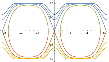
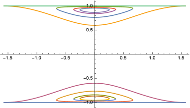
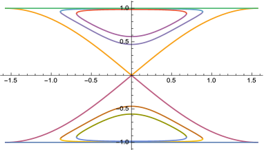
Figure 1: Case $0<{\delta}<1$. ${\tt S}_{\rm 0}({\tt J},{\rm r}^{\prime})$ (left) is inner to ${\tt S}_{\rm 1}({\tt J},{\rm r}^{\prime})$ (right).

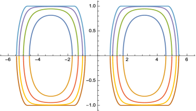
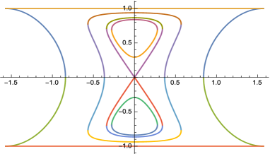
Figure 2: Case ${\delta}=1$. ${\tt S}_{\rm 0}({\tt J},{\rm r}^{\prime})$ (left) and ${\tt S}_{\rm 1}({\tt J},{\rm r}^{\prime})$ (right) coincide.

Figure 3: Case $1<{\delta}<2$. ${\tt S}_{\rm 1}({\tt J},{\rm r}^{\prime})$(left) is inner to ${\tt S}_{\rm 0}({\tt J},{\rm r}^{\prime})$ (right).

The proof of the proposition below is deferred to Section 4.3.1.

Proposition 4.2

The reduced phase space ${\cal M}_{0}({\rm r}^{\prime})$ is includes three open and connected subsets foliated by compact, connected and smooth reduced level sets given by

$${\cal M}^{(j)}_{0}({\rm r}^{\prime})=\bigcup_{({\tt J},{\tt E})\in{\Pi}_{0}^{(j)}({\rm r}^{\prime})}\overline{{\cal C}}_{0,1}({\tt J})\times\overline{{\cal C}}_{0,2}({\tt J},{\tt E},{\rm r}^{\prime})\}\ .$$

The ${\cal M}^{(j)}_{0}({\rm r}^{\prime})$ are delimited by the two separatrices in the reduced phase space ${\cal S}_{\rm 0}({\rm r}^{\prime})$, ${\cal S}_{\rm 1}({\rm r}^{\prime})$, and are in turn foliated by (173). The projected separatrix ${\tt S}_{\rm 0}({\tt J},{\rm r}^{\prime})$ in the projected phase space ${\cal P}_{\rm 0}({\tt J},{\rm r}^{\prime})$ is inner, outer to the projected separatrix ${\tt S}_{\rm 1}({\tt J},{\rm r}^{\prime})$, accordingly to wether $0<{\delta}<1$ or $1<{\delta}<2$, respectively. For ${\delta}=1$, ${\tt S}_{\rm 0}({\tt J},{\rm r}^{\prime})$ and ${\tt S}_{\rm 1}({\tt J},{\rm r}^{\prime})$ coincide. The projected separatrix ${\tt S}_{\rm 0}({\tt J},{\rm r}^{\prime})$ coincides with the ${\rm E}_{0}$–level set to the saddle $({\rm G},{\rm g})=(0,0)$ (see Figures 3, 3 and 3).

Definition 4.3

We say that

$${\tt A}({\rm r}^{\prime}):\qquad{\tt I}=({\tt J},{\tt E})\in{\Pi}^{(j)}({\rm r}^{\prime})\to{\tt A}({\rm r}^{\prime})({\tt I})=\big{(}{\tt L}({\tt J},{\tt E}),{\tt G}({\tt J},{\tt E})\big{)}\in{\cal W}^{(j)}({\rm r}^{\prime})$$

is an action map to a reduced action–angle coordinates (160) if ${\tt A}$ is a diffeomorphism and

$${\tt A}\circ{\rm I}=({\cal L},{\cal G})$$

To prove the second thesis of Proposition 4.1, we first need to show the following result.

Proposition 4.3

It is possible to find reduced action–angle coordinates

$$\begin{array}[]{llllll}\ \ {{\hat{\!\!\!{\cal A}}}_{0}}({\rm r}^{\prime}):&{\cal W}_{0}^{(j)}({\rm r}^{\prime})\times{\mathbb{T}}^{2}&\to{\cal M}^{(j)}_{0}({\rm r}^{\prime})\\ \\ &{\hat{\!\!\!{\cal A}}}_{0}({\rm r}^{\prime})=({\cal L}_{0},{\cal G}_{0},{\lambda}_{0},{\gamma}_{0})&\to\hat{\cal K}=({\Lambda},{\rm G},\ell,{\rm g})\end{array}$$ (177)

equipped with an action map of the form

$${\tt A}_{0}({\rm r}^{\prime})({\tt I})=({\tt L}_{0}({\tt J}),{\tt G}_{0}({\tt J},{\tt E},{\rm r}^{\prime}))$$

where ${\tt E}\in{\Pi}_{0}({\tt J},{\rm r}^{\prime})\to{\tt G}_{0}({\tt J},{\tt E},{\rm r}^{\prime})$ is continuous and increasing on all of ${\Pi}_{0}({\tt J},{\rm r}^{\prime})$.

The main point of this proposition is the continuity of the function ${\tt E}\to{\tt G}_{0}({\tt J},{\tt E},{\rm r}^{\prime})$ for ${\tt E}\in{\Pi}_{0}({\tt J},{\rm r}^{\prime})$, namely, also for ${\tt E}\in\Sigma_{0}({\tt J},{\rm r}^{\prime})$, or $\Sigma_{1}({\tt J},{\rm r}^{\prime})$.

Referring to Section 4.3.3 for the technical details, let us remark, here, the main idea that allows to obtain this continuity. The proof consists of two steps. At the first step, we check that Arnold’s scheme is well defined to this case. As well known, by [1], one first constructs a map

$$\hat{\tt A}_{0}:\quad{\tt I}=({\tt J},{\tt E})\in{\Pi}^{(j)}_{0}({\rm r}^{\prime})\to(\hat{\tt L}_{0}({\tt J}),\hat{\tt G}_{0}({\tt J},{\tt E},{\rm r}^{\prime}))\in{\cal W}^{(j)}_{0}({\rm r}^{\prime})$$ (178)

where $\hat{\tt L}_{0}({\tt J})$ $\hat{\tt G}_{0}({\tt J},{\tt E},{\rm r}^{\prime})$, which we call Arnold actions, are defined, in terms of the integrals ${\tt J}$ and ${\tt E}$ as

$$\hat{\tt L}_{0}({\tt J})={\tt In}[\overline{{\cal C}}_{0,1}({\tt J})]\ ,\qquad\hat{\tt G}_{0}({\tt J},{\tt E},{\rm r}^{\prime})={\tt In}[\overline{{\cal C}}_{0,2}({\tt J},{\tt E},{\rm r}^{\prime})]$$

where ${\tt In}[{\cal C}]$ denotes the area of the inner region delimited by ${\cal C}$, divided by $2{\pi}$. The first equation immediately gives $\hat{\tt L}_{0}({\tt J})={\tt L}_{0}({\tt J})={\Lambda}$, so the problem reduces to the determination of angle coordinate, which we call Arnold angle, associated to the one–degree of freedom Hamiltonian $({\rm G},{\rm g})\to{\rm E}_{0}$ in (171), which, accordingly to [1], is given by

$$\hat{\gamma}_{0}({\Lambda},{\rm G},{\rm g})=2{\pi}\left.\frac{t({\tt J},{\tt E},{\rm r}^{\prime};{\rm G})}{T({\tt J},{\tt E},{\rm r}^{\prime})}\right|_{({\tt J},{\tt E})=({\rm J}_{0}({\Lambda}),{\rm E}_{0}({\Lambda},{\rm G},{\rm g}))}$$ (179)

where, for a given ${\rm G}$ such that $({\rm G},{\rm g})\in$ $\overline{{\cal C}}_{0,2}({\tt J},{\tt E},{\rm r}^{\prime})$ for some ${\rm g}$, $t({\tt J},{\tt E},{\rm r}^{\prime};{\rm G})$ is the time needed to reach $({\rm G},{\rm g})$ on $\overline{{\cal C}}_{0,2}({\tt J},{\tt E},{\rm r}^{\prime})$ and $T({\tt J},{\tt E},{\rm r}^{\prime})$ is the period associated to $\overline{{\cal C}}_{0,2}({\tt J},{\tt E},{\rm r}^{\prime})$. Even though the explicit computation is forbidden, since it involves elliptic integrals, however, it is standard (see Section 4.3.2 for the details) to show that

Proposition 4.4

For all $j=1$, $2$, $3$, the Arnold map (178) is a action map to a reduced action–angle coordinate

$$\hat{\hat{\!\!\!{\cal A}}}_{0}:\quad(\hat{\cal L}_{0},\hat{\cal G}_{0},\hat{\lambda}_{0},\hat{\gamma}_{0})\in{\cal W}^{(j)}_{0}({\rm r}^{\prime})\times{\mathbb{T}}^{2}\to({\Lambda},{\rm G},\ell,{\rm g})\in{\cal M}^{(j)}_{0}({\rm r}^{\prime})$$ (180)

to ${\rm J}_{0}$, where $\hat{\gamma}_{0}$ is as in (179).

To avoid confusion with the symbols defined below, we shall refer to $\hat{\tt A}_{0}$ as Arnold action map and to $\ \hat{\hat{\!\!\!{\cal A}}}_{0}$ as Arnold action–angle coordinates. Indeed, as a the second step for the proof of Proposition 4.3, we introduce a modification of Arnold’s action–angle coordinates, redefining

$${\tt L}_{0}({\tt J})=\hat{\tt L}_{0}({\tt J})$$

and ${\tt G}_{0}({\tt J},{\tt E},{\rm r}^{\prime})$ as follows. If $0<{\delta}\leq 1$:

$${\tt G}_{0}({\tt J},{\tt E},{\rm r}^{\prime}):=\left\{\begin{array}[]{lrr}{\tt In}\Big{[}\overline{{\cal C}}_{0,2}({\tt J},{\tt E},{\rm r}^{\prime})\Big{]}\quad\textrm{ for }-{\delta}<\mathaccent 866{\tt E}<{\delta}\ \textrm{ or }{\delta}<\mathaccent 866{\tt E}<1\\ \\ {\tt Ext}\Big{[}\overline{{\cal C}}_{0,2}({\tt J},{\tt E},{\rm r}^{\prime})\Big{]}\quad\textrm{ for }1<\mathaccent 866{\tt E}<1+\frac{{\delta}^{2}}{4}\end{array}\right.$$ (184)

If $1<{\delta}<2$:

$${\tt G}_{0}({\tt J},{\tt E},{\rm r}^{\prime}):=\left\{\begin{array}[]{lrr}{\tt In}\Big{[}\overline{{\cal C}}_{0,2}({\tt J},{\tt E},{\rm r}^{\prime})\Big{]}\quad\textrm{ for }-{\delta}<\mathaccent 866{\tt E}<1\\ \\ {\tt Ext}\Big{[}\overline{{\cal C}}_{0,2}({\tt J},{\tt E},{\rm r}^{\prime})\Big{]}\quad\textrm{ for }1<\mathaccent 866{\tt E}<{\delta}\quad{\rm or}\quad{\delta}<\mathaccent 866{\tt E}<1+\frac{{\delta}^{2}}{4}\end{array}\right.$$ (188)

where ${\tt Ext}[\overline{{\cal C}}_{0,2}({\tt J},{\tt E},{\rm r}^{\prime})]$ denote the area, normalized to $2{\pi}$, of the complement of the inner region, with respect to the strip $[0,{\Lambda}]$. It is evident from the definition that

Proposition 4.5

The function ${\tt E}\to{\tt G}_{0}({\tt J},{\tt E},{\rm r}^{\prime})$ is continuous on ${\Pi}_{0}({\tt J},{\rm r}^{\prime})$.

The main point that allows this new definition is the relation

$${\tt In}\Big{[}\overline{{\cal C}}_{0,2}({\tt J},{\tt E},{\rm r}^{\prime})\Big{]}+{\tt Ext}\Big{[}\overline{{\cal C}}_{0,2}({\tt J},{\tt E},{\rm r}^{\prime})\Big{]}={\Lambda}={\tt L}_{0}({\tt J})$$ (189)

thanks to which we obtain a new set of coordinates

$$\hat{\!\!\!{\cal A}}_{0}=({\cal L}_{0},{\cal G}_{0},{\lambda}_{0},{\gamma}_{0})$$

such that the coordinates $({\lambda}_{0},{\gamma}_{0})$, naturally and canonically associated to the new actions, are angles too, since they are related to $(\hat{\lambda}_{0},\hat{\gamma}_{0})$ via linear relations with integer coefficients.

We finally turn to full action–angle coordinates to ${\rm J}_{0}$. Let ${\cal W}^{(j)}_{0}({\rm r}^{\prime})$, ${\cal M}^{(j)}_{0}({\rm r}^{\prime})$ be as in Proposition 4.1 and let ${\cal W}^{(j)}_{0}$, ${\cal M}^{(j)}_{0}$ be as in Definition 4.2. A standard procedure (see Section 4.3.5 for details) allows to prove that

Proposition 4.6

It is possible to find full action–angle coordinates ${\cal A}_{0}$ to ${\rm J}_{0}$ with ${\cal W}^{(j)}_{0}({\rm r}^{\prime})$, ${\cal M}^{(j)}_{0}({\rm r}^{\prime})$ as in Proposition 4.1 and ${\cal A}_{0}$ having the form

$${\rm G}={\tt G}_{0}({\cal L}_{0},{\cal G}_{0},{\rm g}_{0},\hat{\rm r}_{0}^{\prime})\ ,\quad{\rm g}={\tt g}_{0}({\cal L}_{0},{\cal G}_{0},{\rm g}_{0},\hat{\rm r}_{0}^{\prime})$$

$${\Lambda}={\cal L}_{0}\ ,\quad\ell={\lambda}_{0}+{\varphi}_{0}({\cal L}_{0},{\cal G}_{0},{\rm g}_{0},\hat{\rm r}_{0}^{\prime})$$

$${\rm R}^{\prime}={\hat{\rm R}}_{0}^{\prime}+{\rho}_{0}({\cal L}_{0},{\cal G}_{0},{\rm g}_{0},\hat{\rm r}_{0}^{\prime})\ ,\quad{\rm r}^{\prime}={\hat{\rm r}}_{0}^{\prime}$$ (190)

4.2 Case ${\mu}>0$, small

The following proposition is proved in Section 4.3.6

Proposition 4.7

For all $j=1$, $2$, $3$ and any compact set ${\tt K}\subset{\Pi}^{(j)}_{0}({\rm r}^{\prime})$ one can find ${\mu}_{0}({\tt K})$ such that, for all $({\tt J},{\tt E})\in{\tt K}$, all $0<{\mu}<{\mu}_{0}({\tt K})$, ${\cal M}_{\mu}({\tt J},{\tt E},{\rm r}^{\prime})$ is smooth, connected and compact.

The previous proposition has the following consequence. Recall the definition of the sets ${\cal W}^{(j)}_{0}({\rm r}^{\prime})$ in (4.1). For a given set $D\subset{\mathbb{R}}^{n}$, denote

$$D_{-{\delta}_{0}}:=\big{\{}{\tt P}\in{\mathbb{R}}^{n}:\ B^{n}_{{\delta}_{0}}({\tt P})\subset D\big{\}}$$

Proposition 4.8

Fix $j=1$, $2$, $3$; ${\delta}_{0}>0$ so small that ${\Pi}^{(j)}({\rm r}^{\prime})_{-2{\delta}_{0}}\neq\emptyset$, and a compact set ${\tt K}\subset{\Pi}^{(j)}({\rm r}^{\prime})_{-2{\delta}_{0}}$. Then it is possible to find ${\mu}_{1}({\delta}_{0},{\tt K})>0$ and ${\cal W}^{(j)}_{{\mu},{\tt K}}({\rm r}^{\prime})\subset{\cal W}^{(j)}_{0}({\rm r}^{\prime})$ such that, if $0<{\mu}<{\mu}_{1}({\delta}_{0},{\tt K})$ and

$${\cal M}^{(j)}_{{\mu},{\tt K}}({\rm r}^{\prime}):=\bigcup_{({\tt J},{\tt E})\in{\tt K}}{\cal M}_{{\mu},{\tt K}}({\tt J},{\tt E},{\rm r}^{\prime})\ ,$$

$({\cal W}^{(j)}_{{\mu},{\tt K}}({\rm r}^{\prime}),{\cal M}^{(j)}_{{\mu},{\tt K}}({\rm r}^{\prime}))$ are Liouville–Arnold domains for ${\rm J}$.

Proof By Proposition 4.7, if $0<{\mu}<{\mu}_{0}({\tt K})$, one can find ${\cal W}^{(j)}_{{\mu},{\tt K}}({\rm r}^{\prime})$ such that $({\cal W}^{(j)}_{{\mu},{\tt K}}({\rm r}^{\prime}),{\cal M}^{(j)}_{{\mu},{\tt K}}({\rm r}^{\prime}))$ are Liouville–Arnold domains for ${\rm J}$. But also, by Proposition 4.1, one can find $\tilde{\cal W}^{(j)}_{0,{\tt K}}({\rm r}^{\prime})\subset{\cal W}^{(j)}_{0}({\rm r}^{\prime})$ such that $(\tilde{\cal W}^{(j)}_{0,{\tt K}}({\rm r}^{\prime}),{\cal M}^{(j)}_{0,{\tt K}}({\rm r}^{\prime}))$ are Liouville–Arnold domains for ${\rm J}_{0}$. Since ${\tt K}\subset{\Pi}^{(j)}_{-2{\delta}_{0}}({\rm r}^{\prime})$, there exists ${\delta}_{1}$ depending on ${\delta}_{0}$ such that $\tilde{\cal W}^{(j)}_{0,{\tt K}}({\rm r}^{\prime})\subset{\cal W}^{(j)}_{0,-2{\delta}_{1}}({\rm r}^{\prime})\subset{\cal W}^{(j)}_{0}({\rm r}^{\prime})$. But $\tilde{\cal W}^{(j)}_{0,{\tt K}}({\rm r}^{\prime})$ is ${\mu}$–close to ${\cal W}^{(j)}_{{\mu},{\tt K}}({\rm r}^{\prime})$, so, for a suitable $0<{\mu}_{1}({\delta}_{0},{\tt K})<{\mu}_{0}({\tt K})$, ${\cal W}^{(j)}_{{\mu},{\tt K}}({\rm r}^{\prime})\subset{\cal W}^{(j)}_{0,-{\delta}_{1}}({\rm r}^{\prime})$, for all $0<{\mu}<{\mu}_{1}({\delta}_{0},{\tt K})$. Since ${\cal W}^{(j)}_{0,-{\delta}_{1}}({\rm r}^{\prime})\subset{\cal W}^{(j)}_{0}({\rm r}^{\prime})$, the theorem is proved.  $\square$

The following Proposition is proved in Section 4.3.6.

Proposition 4.9

Under the assumptions of Proposition 4.7, a diffeomorphism

$$\phi_{\mu}({\tt J},{\tt E},{\rm r}^{\prime}):\quad\psi=(\psi_{1},\psi_{2})\in{\mathbb{T}}^{2}\to{\cal M}_{\mu}({\tt J},{\tt E},{\rm r}^{\prime})$$

can be chosen of the form

$$\phi_{\mu}({\tt J},{\tt E},{\rm r}^{\prime}):\qquad\left\{\begin{array}[]{l}\displaystyle{\Lambda}={\Lambda}_{\mu}({\tt J},{\tt E},{\rm r}^{\prime},\psi_{1},\psi_{2})\\ {\rm G}={\rm G}_{\mu}({\tt J},{\tt E},{\rm r}^{\prime},\psi_{1},\psi_{2})\\ \ell=\psi_{1}\\ {\rm g}={\rm g}_{\mu}({\tt J},{\tt E},{\rm r}^{\prime},\psi_{1},\psi_{2})\end{array}\right.$$

where ${\rm g}_{\mu}$ verifies

$${\rm g}_{\mu}({\tt J},{\tt E},{\rm r}^{\prime},\psi_{1},0)=\frac{1-{\sigma}({\tt J},{\tt E})}{2}{\pi}\ ,\quad\forall\ \psi_{1}\in{\mathbb{T}}$$

with ${\sigma}({\tt J},{\tt E}):=\left\{\begin{array}[]{l}-1\quad-{\delta}<\mathaccent 866{\tt E}<1\\ +1\quad 1<\mathaccent 866{\tt E}<1+\frac{{\delta}^{2}}{4}\ .\\ \end{array}\right.$

We define the base circles

$${\cal C}_{1,{\mu}}:=\phi_{\mu}({\tt J},{\tt E},{\rm r}^{\prime})({\mathbb{T}}\times\{0\}_{\rm mod\ 2{\pi}})\ ,\quad{\cal C}_{2,{\mu}}:=\phi_{\mu}({\tt J},{\tt E},{\rm r}^{\prime})(\{0\}_{\rm mod\ 2{\pi}}\times{\mathbb{T}})$$

which have parametric equation

$${\cal C}_{1,{\mu}}({\tt J},{\tt E},{\rm r}^{\prime}):\quad\left\{\begin{array}[]{l}\displaystyle{\Lambda}={\Lambda}_{{\mu},1}({\tt J},{\tt E},{\rm r}^{\prime},\psi_{1})\\ {\rm G}={\rm G}_{{\mu},1}({\tt J},{\tt E},{\rm r}^{\prime},\psi_{1})\\ \ell=\psi_{1}\\ {\rm g}=\frac{1-{\sigma}}{2}{\pi}\end{array}\right.\qquad\psi_{1}\in{\mathbb{T}}$$

$${\cal C}_{2,{\mu}}({\tt J},{\tt E},{\rm r}^{\prime}):\quad\left\{\begin{array}[]{l}\displaystyle{\Lambda}={\Lambda}_{{\mu},2}({\tt J},{\tt E},{\rm r}^{\prime},\psi_{2})\\ {\rm G}={\rm G}_{{\mu},2}({\tt J},{\tt E},{\rm r}^{\prime},\psi_{2})\\ \ell=0\\ {\rm g}={\rm g}_{{\mu},2}({\tt J},{\tt E},{\rm r}^{\prime},\psi_{2})\end{array}\right.\qquad\psi_{2}\in{\mathbb{T}}$$

Then we define, analogously to the case ${\mu}=0$, the Arnold actions

$$\hat{\tt L}_{\mu}:={\tt In}[{\cal C}_{1,{\mu}}]=\frac{1}{2{\pi}}\int_{{\cal C}_{1}}({\Lambda}d\ell+{\rm G}d{\rm g})=\frac{1}{2{\pi}}\int_{\overline{{\cal C}}_{1,{\mu}}}{\Lambda}d\ell={\tt In}[\overline{{\cal C}}_{1,{\mu}}]$$

$$\hat{\tt G}_{\mu}:={\tt In}[{\cal C}_{2,{\mu}}]=\frac{1}{2{\pi}}\int_{{\cal C}_{2}}({\Lambda}d\ell+{\rm G}d{\rm g})=\frac{1}{2{\pi}}\int_{\overline{{\cal C}}_{2,{\mu}}}{\rm G}d{\rm g}={\tt In}[\overline{{\cal C}}_{2,{\mu}}]$$

where we have introduced the projected curves $\overline{{\cal C}}_{1,{\mu}}$, $\overline{{\cal C}}_{2,{\mu}}$

$$\overline{{\cal C}}_{1,{\mu}}:\quad\left\{\begin{array}[]{l}{\Lambda}={\Lambda}_{{\mu},1}({\tt J},{\tt E},{\rm r}^{\prime},\psi_{1})\\ \ell=\psi_{1}\end{array}\right.\qquad\overline{{\cal C}}_{2,{\mu}}:\quad\left\{\begin{array}[]{l}{\rm G}={\rm G}_{{\mu},2}({\tt J},{\tt E},{\rm r}^{\prime},\psi_{2})\\ {\rm g}={\rm g}_{{\mu},2}({\tt J},{\tt E},{\rm r}^{\prime},\psi_{2})\end{array}\right.$$

and we have used the fact that ${\rm g}$ (respectively, $\ell$) is constant along ${\cal C}_{1,{\mu}}$ (respectively, ${\cal C}_{2,{\mu}}$).

Similarly to the case ${\mu}=0$, we define the Arnold map

$$\hat{\tt A}:\quad({\tt J},{\tt E})\in{\Pi}^{(j)}_{{\mu},{\tt K}}({\rm r}^{\prime})\to(\hat{\tt L}_{\mu},\hat{\tt G}_{\mu})\in{\cal W}^{(j)}_{{\mu},{\tt K}}({\rm r}^{\prime}):=\hat{\tt A}({\Pi}^{(j)}_{{\mu},{\tt K}}({\rm r}^{\prime}))$$ (192)

The following statement is of the same kind of an analogue result (Proposition 4.4) given for ${\mu}=0$, but it is actually weker.: here continuity in ${\tt E}$ is not discussed, since the involved domains ${\cal W}^{(j)}_{{\mu},{\tt K}}$, ${\cal M}^{(j)}_{{\mu},{\tt K}}$ are deprived of a neighborhood of their boundaries. However, there is continuity in ${\mu}$. The proof is omitted, since it is an immediate consequence of the Implicit Function Theorem.

Proposition 4.10

For all ${\tt K}$, all $j=1$, $2$, $3$, the Arnold map (192) is a action map to a reduced action–angle coordinate

$${{{\!\!\!{\cal A}}_{\mu}}}:\quad({\cal L},{\cal G},{\lambda},{\gamma})\in{\cal W}^{(j)}_{{\mu},{\tt K}}({\rm r}^{\prime})\times{\mathbb{T}}^{2} \to({\Lambda},{\rm G},\ell,{\rm g})\in{\cal M}^{(j)}_{{\mu},{\tt K}}({\rm r}^{\prime})$$

to ${\rm J}$, which reduce to $\ {\!\!\!{\cal A}}_{0}$ as ${\mu}\to 0$.

We finally turn to full action–angle coordinates. For given $j$, ${\delta}_{0}$, ${\tt K}$, we denote ${\cal W}^{(j)}_{{\mu},{\tt K}}=\cup_{{\rm r}^{\prime}>0}{\cal W}^{(j)}_{{\mu},{\tt K}}({\rm r}^{\prime})$, ${\cal M}^{(j)}_{{\mu},{\tt K}}=\cup_{{\rm r}^{\prime}>0}{\cal M}^{(j)}_{{\mu},{\tt K}}({\rm r}^{\prime})$. The following proposition is proved in Section 4.3.6.

Proposition 4.11

It is possible to find full action–angle coordinates ${\cal A}_{\mu}:\ {\cal W}^{(j)}_{{\mu},{\tt K}}\to{\cal M}^{(j)}_{{\mu},{\tt K}}$, having the form

$${\Lambda}={\tt{\Lambda}}_{\mu}({\cal L},{\cal G},{\lambda},{\gamma},{\hat{\rm r}}^{\prime})\ ,\quad{\rm G}={\tt G}_{\mu}({\cal L},{\cal G},{\lambda},{\gamma},{\hat{\rm r}}^{\prime})$$

$$\ell={\tt l}_{\mu}({\cal L},{\cal G},{\lambda},{\gamma},{\hat{\rm r}}^{\prime})\ ,\quad{\rm g}={\tt g}_{\mu}({\cal L},{\cal G},{\lambda},{\gamma},{\hat{\rm r}}^{\prime})$$

$${\rm R}^{\prime}={\hat{\rm R}}^{\prime}+\hat{\rho}({\cal L},{\cal G},{\lambda},{\gamma},{\hat{\rm r}}^{\prime})\ ,\quad{\rm r}^{\prime}={\hat{\rm r}}^{\prime}$$ (193)

Remark 4.1

We remark that, since ${\cal A}_{\mu}$ is ${\mu}$–close to the transformation ${\cal A}_{0}$, then the function ${\rm J}_{{\cal A}_{\mu}}:={\rm J}\circ{\cal A}_{\mu}$ has the form

$${\rm J}_{{\cal A}_{\mu}}({\cal L},{\cal G},\hat{\rm r}^{\prime};{\mu})=-\frac{{\rm m}^{3}{\cal M}^{2}}{2{\cal L}^{2}}+{\mu}{\rm U}({\cal L},{\cal G},\hat{\rm r}^{\prime};{\mu})\ .$$ (194)

We shall use this in the next Section 5.

We conclude this section with providing, for completeness, the analytical expression of $\overline{{\cal C}}_{1,{\mu}}$ and $\overline{{\cal C}}_{2,{\mu}}$, even though it will be not used in the paper. The proof of the following proposition is given Section 4.3.6.

Proposition 4.12

$\overline{{\cal C}}_{1,{\mu}}({\tt J},{\tt E},{\rm r}^{\prime})$ is the projection in the plane $({\Lambda},\ell)$ of the curve in the space $({\Lambda},{\rm G},\ell)$ defined by equations

$$\left\{\begin{array}[]{l}\displaystyle-\frac{{\rm m}^{3}{\cal M}^{2}}{2{\Lambda}^{2}}-{\mu}\frac{{\rm m}{\cal M}}{\sqrt{{{\rm r}^{\prime}}^{2}-2{\rm r}^{\prime}{\sigma}a\varrho\cos{\nu}+{a}^{2}\varrho^{2}}}={\rm J}\\ \\ \displaystyle{\rm G}^{2}-{\sigma}{\rm m}^{2}{\cal M}{\rm r}^{\prime}\sqrt{1-\frac{{\rm G}^{2}}{{\Lambda}^{2}}}+{\mu}{\rm m}^{2}{\cal M}{\rm r}^{\prime}\frac{{{\rm r}^{\prime}}-{\sigma}a\varrho\cos{\nu}}{\sqrt{{{\rm r}^{\prime}}^{2}-2{\rm r}^{\prime}{\sigma}a\varrho\cos{\nu}+{a}^{2}\varrho^{2}}}={\rm E}\end{array}\right.$$ (198)

$\overline{{\cal C}}_{2,{\mu}}({\tt J},{\tt E},{\rm r}^{\prime})$ is the projection in the plane $({\rm g},{\rm G})$ of the curve in the space $({\Lambda},{\rm G},{\rm g})$ defined by equations

$$\left\{\begin{array}[]{l}\displaystyle-\frac{{\rm m}^{3}{\cal M}^{2}}{2{\Lambda}^{2}}-{\mu}\frac{{\rm m}{\cal M}}{\sqrt{{{\rm r}^{\prime}}^{2}+2{\rm r}^{\prime}a(1-{\rm e})\cos{\rm g}+{a}^{2}(1-{\rm e})^{2}}}={\tt J}\\ \\ \displaystyle{\rm G}^{2}+{\rm m}^{2}{\cal M}{\rm r}^{\prime}\sqrt{1-\frac{{\rm G}^{2}}{{\Lambda}^{2}}}\cos{\rm g}+{\mu}{\rm m}^{2}{\cal M}{\rm r}^{\prime}\frac{{{\rm r}^{\prime}}+a(1-{\rm e})\cos{\rm g}}{\sqrt{{{\rm r}^{\prime}}^{2}+2{\rm r}^{\prime}a(1-{\rm e})\cos{\rm g}+{a}^{2}(1-{\rm e})^{2}}}\\ \qquad\qquad\qquad\qquad\qquad={\tt E}\end{array}\right.$$ (203)

4.3 Proofs

4.3.1 Proof of Proposition 4.2

The first part of the proof of Proposition 4.2 consists in proving that

Proposition 4.13

For any $j=1$, $2$, $3$, any ${\tt E}\in{\Pi}_{0}^{(j)}({\tt J},{\rm r}^{\prime})$, the level sets $\overline{{\cal C}}_{0,2}({\tt J},{\tt E},{\rm r}^{\prime})$ defined by equation (171) are smooth, connected and compact curves, consisting of the union of graphs

$$\overline{{\cal C}}_{2,0,\pm}({\tt J},{\tt E},{\rm r}^{\prime}):\quad\left\{\begin{array}[]{l}\displaystyle{\Lambda}={\tt L}_{0}({\tt J})\\ {\rm g}=\pm\overline{\rm g}_{0}({\tt J},{\tt E},{\rm r}^{\prime},{\rm G}^{\prime})\quad\mod\ 2{\pi}\\ \ell\in{\mathbb{T}}\\ {\rm G}^{\prime}\in\overline{{\cal F}}_{0}({\tt J},{\tt E},{\rm r}^{\prime})\end{array}\right.$$ (208)

Proof To simplify notations, we divide this equation by ${\tt L}_{0}({\tt J})^{2}$, and we rewrite it as

$$\mathaccent 866{{\rm E}}_{0}(\mathaccent 866{{\rm G}},{\rm g})=\mathaccent 866{{\rm G}}^{2}+{\delta}\sqrt{1-\mathaccent 866{{\rm G}}^{2}}\cos{\rm g}=\mathaccent 866{\tt E}\ ,$$ (209)

where

$$\mathaccent 866{{\rm E}}_{0}(\mathaccent 866{{\rm G}},{\rm g}):=\frac{{\rm E}_{0}({\tt L}_{0}({\tt J})^{2}\mathaccent 866{{\rm G}},{\rm g})}{{\tt L}_{0}({\tt J})^{2}}\ ,\quad\mathaccent 866{\tt E}:=\frac{{\tt E}}{{\tt L}_{0}({\tt J})^{2}}\ ,\quad\mathaccent 866{{\rm G}}:=\frac{{\rm G}}{{\tt L}_{0}({\tt J})}$$

$${\delta}={\rm m}^{2}{\cal M}\frac{{\rm r}^{\prime}}{{\tt L}_{0}({\tt J})^{2}}$$ (210)

and we study the rescaled level sets (209) in the plane $({\rm g},\mathaccent 866{{\rm G}})$. For ${\delta}\in(0,2)$, $\mathaccent 866{{\rm E}}_{0}$ has a minimum, a saddle and a maximum, respectively at

$$\hat{\tt P}_{-}=({\pi},0)\ ,\qquad\hat{\tt P}_{0}=(0,0)\ ,\qquad\hat{\tt P}_{+}=(0,\sqrt{1-\frac{{\delta}^{2}}{4}})$$

where it takes the values, respectively,

$$\mathaccent 866{{\rm E}}_{0-}=-{\delta}\ ,\qquad\mathaccent 866{{\rm E}}_{0\rm sad}={\delta}\ ,\quad\mathaccent 866{{\rm E}}_{0+}=1+\frac{{\delta}^{2}}{4}\ .$$

Thus, we study the level sets (4.3.1) for

$$\mathaccent 866{\tt E}\in\left[-{\delta},1+\frac{{\delta}^{2}}{4}\right]\ .$$ (211)

We solve for ${\rm g}$:

$${\rm g}={\rm g}_{\pm}=\pm\cos^{-1}\left(\frac{\mathaccent 866{\tt E}-\mathaccent 866{{\rm G}}^{2}}{{\delta}\sqrt{1-\mathaccent 866{{\rm G}}^{2}}}\right)\quad\mod\ 2{\pi}\ .$$ (212)

Using

$$1-\left(\frac{\mathaccent 866{\tt E}-\mathaccent 866{{\rm G}}^{2}}{{\delta}\sqrt{1-\mathaccent 866{{\rm G}}^{2}}}\right)^{2}=\frac{{\delta}^{2}-\mathaccent 866{\tt E}^{2}-2(\frac{{\delta}^{2}}{2}-\mathaccent 866{\tt E})\mathaccent 866{{\rm G}}^{2}-\mathaccent 866{{\rm G}}^{4}}{{\delta}^{2}(1-\mathaccent 866{{\rm G}}^{2})}=\frac{(\mathaccent 866{{\rm G}}^{2}-\mathaccent 866{{\rm G}}_{-}^{2})(\mathaccent 866{{\rm G}}_{+}^{2}-\mathaccent 866{{\rm G}}^{2})}{{\delta}^{2}(1-\mathaccent 866{{\rm G}}^{2})}$$ (213)

with

$$\mathaccent 866{{\rm G}}^{2}_{\pm} = \mathaccent 866{\tt E}-\frac{{\delta}^{2}}{2}\pm\sqrt{\big{(}\mathaccent 866{\tt E}-\frac{{\delta}^{2}}{2}\big{)}^{2}+{\delta}^{2}-\mathaccent 866{\tt E}^{2}}$$ (214)

$$= \mathaccent 866{\tt E}-\frac{{\delta}^{2}}{2}\pm{\delta}\sqrt{1+\frac{{\delta}^{2}}{4}-\mathaccent 866{\tt E}}$$

one sees the the equality (212) is well defined for

$$\mathaccent 866{{\rm G}}_{\rm min}\leq\mathaccent 866{{\rm G}}\leq\mathaccent 866{{\rm G}}_{\rm max}$$ (215)

where

$$\mathaccent 866{{\rm G}}^{2}_{\rm min}:=\max\{\mathaccent 866{{\rm G}}^{2}_{-},0\}\ ,\qquad\mathaccent 866{{\rm G}}^{2}_{\rm max}:=\min\{\mathaccent 866{{\rm G}}^{2}_{+},1\}\ .$$

Note that, when $\mathaccent 866{\tt E}$ takes its maximum value $1+\frac{{\delta}^{2}}{4}$, one has $\mathaccent 866{{\rm G}}_{+}^{2}=\mathaccent 866{{\rm G}}_{-}^{2}=1-\frac{{\delta}^{2}}{4}$. Therefore, by (212) and (215), the level set with $\mathaccent 866{\tt E}=1+\frac{{\delta}^{2}}{4}$ reduces to the maximum point $(0,\pm\sqrt{1-\frac{{\delta}^{2}}{4}})$. Writing

$$\mathaccent 866{{\rm G}}_{-}^{2}=\frac{\mathaccent 866{\tt E}^{2}-{\delta}^{2}}{\mathaccent 866{\tt E}-\frac{{\delta}^{2}}{2}+{\delta}\sqrt{1+\frac{{\delta}^{2}}{4}-\mathaccent 866{\tt E}}}$$

and noticing that

$$1-\mathaccent 866{{\rm G}}_{+}^{2}=1-\left(\mathaccent 866{\tt E}-\frac{{\delta}^{2}}{2}+{\delta}\sqrt{1+\frac{{\delta}^{2}}{4}-\mathaccent 866{\tt E}}\right)=\left(\frac{{\delta}}{2}-\sqrt{1+\frac{{\delta}^{2}}{4}-\mathaccent 866{\tt E}}\right)^{2}\geq 0\ ,$$

one finds that

$$\mathaccent 866{{\rm G}}_{\rm min}=\left\{\begin{array}[]{l}0\qquad{\rm if}\quad-{\delta}\leq\mathaccent 866{\tt E}\leq{\delta}\\ \mathaccent 866{{\rm G}}_{-}\quad{\rm if}\quad\mathaccent 866{\tt E}>{\delta}\end{array}\right.\ ,\qquad\mathaccent 866{{\rm G}}_{\rm max}=\mathaccent 866{{\rm G}}_{+}\ .$$ (218)

Observe that

$$\lim_{\mathaccent 866{\tt E}\to{\delta}}{\rm G}^{2}_{\rm min}=\lim_{\mathaccent 866{\tt E}\to{\delta}}{\rm G}^{2}_{-}=0\ ,\quad\lim_{\mathaccent 866{\tt E}\to{\delta}}{\rm G}^{2}_{\rm max}=\lim_{\mathaccent 866{\tt E}\to{\delta}}{\rm G}^{2}_{\rm+}={\delta}(2-{\delta})$$ (219)

and

$$\lim_{\mathaccent 866{\tt E}\to 1}{\rm G}^{2}_{\rm max}=\lim_{\mathaccent 866{\tt E}\to 1}{\rm G}^{2}_{+}=1\ ,\quad\lim_{\mathaccent 866{\tt E}\to 1}\mathaccent 866{{\rm G}}_{-}^{2}=1-{\delta}^{2}\ ,\quad\lim_{\mathaccent 866{\tt E}\to 1}\mathaccent 866{{\rm G}}_{\rm min}^{2}=\max\{1-{\delta}^{2},0\}\ ,$$ (220)

which are obtained using

$$\lim_{\mathaccent 866{\tt E}\to{\delta}}\mathaccent 866{{\rm G}}_{\pm}^{2}={\delta}-\frac{{\delta}^{2}}{2}\pm{\delta}\left(1-\frac{{\delta}}{2}\right)\ ,\quad\lim_{\mathaccent 866{\tt E}\to 1}\mathaccent 866{{\rm G}}^{2}_{\pm}=1-\frac{{\delta}^{2}}{2}\pm\frac{{\delta}^{2}}{2}$$

in turn implied by (214).
In particular, ${\rm G}_{\rm min}$, is continuous for $\mathaccent 866{\tt E}={\delta}$. The inequality (215) defines a “symmetric” domain of $\mathaccent 866{{\rm G}}$ with respect to the origin, consisting of the union

$$\mathaccent 866{{\cal D}}=\mathaccent 866{{\cal D}}_{-}\cup\mathaccent 866{{\cal D}}_{+}$$ (221)

of two “symmetric” intervals

$$\mathaccent 866{{\cal D}}_{-}=\left[-\mathaccent 866{{\rm G}}_{\rm max}\,-\mathaccent 866{{\rm G}}_{\rm min}\right]\ ,\qquad\mathaccent 866{{\cal D}}_{+}=\left[\mathaccent 866{{\rm G}}_{\rm min}\,\mathaccent 866{{\rm G}}_{\rm max}\right]\ .$$

Observe that, for $\mathaccent 866{\tt E}>{\delta}$ and $\mathaccent 866{\tt E}\neq 1$, the union (221) is disjoint, since, in this case, $\mathaccent 866{{\rm G}}_{\rm min}>0$ (se (218)). The functions ${\rm g}_{\pm}$ in (212) are even functions of $\mathaccent 866{{\rm G}}$ on such “symmetric” domain. By construction, ${\cal M}_{0}({\tt J},{\tt E},{\rm r}^{\prime})$ can be recovered as the union of graphs of ${\rm g}_{\sigma}$ for $\mathaccent 866{{\rm G}}\in\mathaccent 866{{\cal D}}_{{\sigma}^{\prime}}$, where ${\sigma}$, ${\sigma}^{\prime}=\pm$. We denote such graphs as ${\cal F}_{{\sigma}{\sigma}^{\prime}}$. The equality (213) implies that

$$\partial_{\rm g}(\mathaccent 866{{\rm E}}_{0}-{\tt E})\Big{|}_{{{\cal F}}_{{\sigma}{\sigma}^{\prime}}}=-{\delta}\sqrt{1-\mathaccent 866{{\rm G}}^{2}}\sin{\rm g}_{\sigma}=-{\sigma}\sqrt{(\mathaccent 866{{\rm G}}^{2}-\mathaccent 866{{\rm G}}_{-}^{2})(\mathaccent 866{{\rm G}}_{+}^{2}-\mathaccent 866{{\rm G}}^{2})}\ .$$

It vanishes only at the extremal points of $\mathaccent 866{{\cal D}}_{{\sigma}^{\prime}}$. Therefore, denoting as $\mathaccent 866{{\cal F}}^{\circ}_{{\sigma}{\sigma}^{\prime}}$ the restriction of $\mathaccent 866{{\cal F}}_{{\sigma}{\sigma}^{\prime}}$ to a pre–fixed compact sub–domain $\mathaccent 866{{\cal D}}_{{\sigma}^{\prime}}^{\circ}\subset\mathaccent 866{{\cal D}}_{{\sigma}^{\prime}}$ which does not include such extremal points, condition (252) is immediately met by $\mathaccent 866{{\cal F}}^{\circ}_{{\sigma}{\sigma}^{\prime}}$.

Completion of the proof of Proposition 4.2 We now turn to study the curves in (209) in the plane $({\rm g},\mathaccent 866{{\rm G}})$, for $\mathaccent 866{\tt E}$ as in (211). By symmetry, we limit to study the behavior of ${\rm g}_{+}$ for $\mathaccent 866{{\rm G}}\in\mathaccent 866{{\cal D}}_{+}$. We denote as

$$\underline{\rm g}:=\cos^{-1}\left(\frac{\mathaccent 866{\tt E}-\mathaccent 866{{\rm G}}_{\rm min}^{2}}{{\delta}\sqrt{1-\mathaccent 866{{\rm G}}_{\rm min}^{2}}}\right)\ ,\quad\overline{\rm g}:=\cos^{-1}\left(\frac{\mathaccent 866{\tt E}-\mathaccent 866{{\rm G}}_{\rm max}^{2}}{{\delta}\sqrt{1-\mathaccent 866{{\rm G}}_{\rm max}^{2}}}\right)$$ (222)

the values that ${\rm g}_{+}$ takes at the extrema of $\mathaccent 866{{\cal D}}_{+}$. The explicit value of $\underline{\rm g}$, $\overline{\rm g}$ is

$$\underline{\rm g}=\left\{\begin{array}[]{l}0\qquad\qquad\ \ {\rm if}\qquad\qquad\mathaccent 866{\tt E}>{\delta}\\ \cos^{-1}\frac{\mathaccent 866{\tt E}}{{\delta}}\qquad{\rm if}\quad-{\delta}\leq\mathaccent 866{\tt E}\leq{\delta}\end{array}\right.\ ,\qquad\overline{\rm g}=\left\{\begin{array}[]{l}{\pi}\quad{\rm if}\quad\mathaccent 866{\tt E}<1\\ \frac{{\pi}}{2}\quad{\rm if}\quad\mathaccent 866{\tt E}=1\\ 0\quad{\rm if}\quad\mathaccent 866{\tt E}>1\end{array}\right.$$ (228)

This follows from the definitions in (214) and (218). In particular, from (214) one finds, for $({\sigma},\mathaccent 866{\tt E})\neq(+,1)$

$$\frac{\mathaccent 866{\tt E}-\mathaccent 866{{\rm G}}_{{\sigma}}^{2}}{{\delta}\sqrt{1-\mathaccent 866{{\rm G}}_{{\sigma}}^{2}}} = \frac{\mathaccent 866{\tt E}-\left(\mathaccent 866{\tt E}-\frac{{\delta}^{2}}{2}+{\sigma}{\delta}\sqrt{1+\frac{{\delta}^{2}}{4}-\mathaccent 866{\tt E}}\right)}{{\delta}\sqrt{1-\left(\mathaccent 866{\tt E}-\frac{{\delta}^{2}}{2}+{\sigma}{\delta}\sqrt{1+\frac{{\delta}^{2}}{4}-\mathaccent 866{\tt E}}\right)}}$$

$$= {\,\rm sign\,}\left(\frac{{\delta}}{2}-{\sigma}\sqrt{1+\frac{{\delta}^{2}}{4}-\mathaccent 866{\tt E}}\right)$$

$$= \left\{\begin{array}[]{l}+1\quad{\rm for}\quad{\sigma}=-\\ -1\quad{\rm for}\quad{\sigma}=+\ \&\ \mathaccent 866{\tt E}<1\\ +1\quad{\rm for}\quad{\sigma}=+\ \&\ \mathaccent 866{\tt E}>1\end{array}\right.$$

while, for $({\sigma},\mathaccent 866{\tt E})=(+,1)$,

$$\frac{\mathaccent 866{\tt E}-\mathaccent 866{{\rm G}}_{+}^{2}}{{\delta}\sqrt{1-\mathaccent 866{{\rm G}}_{+}^{2}}} = \frac{\sqrt{1-\mathaccent 866{{\rm G}}_{+}^{2}}}{{\delta}}=\frac{\sqrt{1-\left(1-\frac{{\delta}^{2}}{2}+{\delta}\sqrt{1+\frac{{\delta}^{2}}{4}-1}\right)}}{{\delta}}=0$$

Let us study the graph of ${\rm g}_{+}$ as a function of $\mathaccent 866{{\rm G}}$, for $\mathaccent 866{{\rm G}}\in\mathaccent 866{{\cal D}}_{+}$. From the formula

$$\partial_{\mathaccent 866{{\rm G}}}{\rm g}_{+}=\frac{\mathaccent 866{{\rm G}}}{\sqrt{(\mathaccent 866{{\rm G}}^{2}-\mathaccent 866{{\rm G}}^{2}_{-})(\mathaccent 866{{\rm G}}^{2}_{\rm max}-\mathaccent 866{{\rm G}}^{2})}}\frac{2-\mathaccent 866{\tt E}-\mathaccent 866{{\rm G}}^{2}}{1-\mathaccent 866{{\rm G}}^{2}}\ .$$ (230)

one sees that $\mathaccent 866{{\rm G}}=\mathaccent 866{{\rm G}}_{0}:=\sqrt{2-\mathaccent 866{\tt E}}\notin\mathaccent 866{{\cal D}}_{+}$ is an extremal point, as soon as $\mathaccent 866{{\rm G}}_{0}\in\mathaccent 866{{\cal D}}_{+}$. Using

$$\mathaccent 866{{\rm G}}_{0}^{2}-\mathaccent 866{{\rm G}}_{\rm max}^{2} = 2-\mathaccent 866{\tt E}-\left(\mathaccent 866{\tt E}-\frac{{\delta}^{2}}{2}+{\delta}\sqrt{1+\frac{{\delta}^{2}}{4}-\mathaccent 866{\tt E}}\right)$$ (231)

$$= \sqrt{1+\frac{{\delta}^{2}}{4}-\mathaccent 866{\tt E}}\left(2\sqrt{1+\frac{{\delta}^{2}}{4}-\mathaccent 866{\tt E}}-{\delta}\right)$$

$$= 2\frac{\sqrt{1+\frac{{\delta}^{2}}{4}-\mathaccent 866{\tt E}}}{\sqrt{1+\frac{{\delta}^{2}}{4}-\mathaccent 866{\tt E}}+{\delta}}(1-\mathaccent 866{\tt E})$$

and

$$\mathaccent 866{{\rm G}}_{0}^{2}-\mathaccent 866{{\rm G}}_{\rm min}^{2} \geq 2-\mathaccent 866{\tt E}-\left(\mathaccent 866{\tt E}-\frac{{\delta}^{2}}{2}-{\delta}\sqrt{1+\frac{{\delta}^{2}}{4}-\mathaccent 866{\tt E}}\right)$$

$$= \sqrt{1+\frac{{\delta}^{2}}{4}-\mathaccent 866{\tt E}}\left(2\sqrt{1+\frac{{\delta}^{2}}{4}-\mathaccent 866{\tt E}}+{\delta}\right)\geq 0\ .$$

we see that

$${\rm g}_{0}\left\{\begin{array}[]{l}\geq\mathaccent 866{{\rm G}}_{\rm max}\quad{\rm for}\quad\mathaccent 866{\tt E}<1\\ \in\mathaccent 866{{\cal D}}_{+}\quad{\rm for}\quad\mathaccent 866{\tt E}\geq 1\end{array}\right.\ .$$

As a consequence,

• For $\mathaccent 866{\tt E}<1$, $\mathaccent 866{{\rm G}}_{0}>\mathaccent 866{{\rm G}}_{\rm max}$ and hence ${\rm g}_{+}$ increases, in $\mathaccent 866{{\cal D}}_{+}$, from $\underline{\rm g}$ to $\overline{\rm g}$.

• For $\mathaccent 866{\tt E}>1$, ${\rm g}_{+}$ increases from $\underline{\rm g}$ to ${\rm g}_{0}$ for $\mathaccent 866{{\rm G}}_{\rm min}\leq\mathaccent 866{{\rm G}}\leq\mathaccent 866{{\rm G}}_{0}$ and decreases from ${\rm g}_{0}$ to $\overline{\rm g}$, for $\mathaccent 866{{\rm G}}_{0}\leq\mathaccent 866{{\rm G}}\leq\mathaccent 866{{\rm G}}_{\rm max}$.

Collecting these informations, the phase portrait of $\mathaccent 866{\tt E}$ in the plane $({\rm g},\mathaccent 866{{\rm G}})$ can be summarized as follows (see also Figures 3, 3 and 3).

• For $0<{\delta}<1$:

  • For $-{\delta}\leq\mathaccent 866{\tt E}<{\delta}$ ${\rm g}$ “librates” around ${\pi}$, with maximum elongation in $[\cos^{-1}\frac{\mathaccent 866{\tt E}}{{\delta}},2{\pi}-\cos^{-1}\frac{\mathaccent 866{\tt E}}{{\delta}}]$;

  • $\mathaccent 866{\tt E}={\delta}$ is the level set through the saddle (separatrix);

  • For ${\delta}<\mathaccent 866{\tt E}<1$, ${\rm g}$ “rotates”, namely takes all the values in ${\mathbb{T}}$.

  • The curve $\mathaccent 866{\tt E}=1$ splits into $\mathaccent 866{{\rm G}}=1$ and $\mathaccent 866{{\rm G}}=\sqrt{1-{\delta}^{2}\cos^{2}{\rm g}}$, with ${\rm g}\in{\mathbb{T}}$. Such two branches glue smoothly at $(\pm\frac{{\pi}}{2},1)$, with ${\rm g}$ mod $2{\pi}$.

  • For $1<\mathaccent 866{\tt E}\leq 1+\frac{{\delta}^{2}}{4}$, ${\rm g}$ librates around $0$, with maximum elongation

    $$[-\frac{2}{{\delta}}\sqrt{\mathaccent 866{\tt E}-1},\frac{2}{{\delta}}\sqrt{\mathaccent 866{\tt E}-1}]\ .$$

• For ${\delta}=1$:

  • For $-1\leq\mathaccent 866{\tt E}<1$ ${\rm g}$ “librates” around ${\pi}$, with maximum elongation in $[\cos^{-1}\mathaccent 866{\tt E},2{\pi}-\cos^{-1}\mathaccent 866{\tt E}]$;

  • $\mathaccent 866{\tt E}=1$ is the level set through the saddle (separatrix). It splits into $\mathaccent 866{{\rm G}}=1$ and $\mathaccent 866{{\rm G}}=|\sin{\rm g}|$, with ${\rm g}\in{\mathbb{T}}$. Such two branches glue smoothly at $(\pm\frac{{\pi}}{2},1)$, with ${\rm g}$ mod $2{\pi}$.

  • For $1<\mathaccent 866{\tt E}<\frac{5}{4}$, ${\rm g}$ librates around $0$, with maximum elongation

    $$[-2\sqrt{\mathaccent 866{\tt E}-1},2\sqrt{\mathaccent 866{\tt E}-1}]\ .$$

• For $1<{\delta}<2$:

  • For $-{\delta}\leq\mathaccent 866{\tt E}<1$ ${\rm g}$ “librates” around ${\pi}$, with maximum elongation in $[\cos^{-1}\frac{\mathaccent 866{\tt E}}{{\delta}},2{\pi}-\cos^{-1}\frac{\mathaccent 866{\tt E}}{{\delta}}]$;

  • the curve $\mathaccent 866{\tt E}=1$ splits into $\mathaccent 866{{\rm G}}=1$ and $\mathaccent 866{{\rm G}}=\sqrt{1-{\delta}^{2}\cos^{2}{\rm g}}$, for $-{\pi}\leq{\rm g}\leq\cos^{-1}\frac{1}{{\delta}}$. Such two branches glue smoothly at $(\pm\frac{{\pi}}{2},1)$, with ${\rm g}$ mod $2{\pi}$.

  • For $1<\mathaccent 866{\tt E}<{\delta}$, ${\rm g}$ “librates” around $0$ with maximum elongation

    $$[-\frac{2}{{\delta}}\sqrt{\mathaccent 866{\tt E}-1},\frac{2}{{\delta}}\sqrt{\mathaccent 866{\tt E}-1}]\ .$$

  • $\mathaccent 866{\tt E}={\delta}$ is the level set through the saddle $(0,0)$ (separatrix)

  • For ${\delta}<\mathaccent 866{\tt E}\leq 1+\frac{{\delta}^{2}}{4}$, ${\rm g}$ librates around $0$, with maximum elongation $[-\frac{2}{{\delta}}\sqrt{\mathaccent 866{\tt E}-1},\frac{2}{{\delta}}\sqrt{\mathaccent 866{\tt E}-1}]$.

  Finally, the analysis of $\partial_{\mathaccent 866{{\rm G}}}{\rm g}_{+}$ in (230) allows to infer that the curves in (209) are smooth for $\mathaccent 866{\tt E}\notin\{\pm{\delta},\ 1,\ 1+\frac{{\delta}^{2}}{4}\}$, as claimed.

4.3.2 Proof of Proposition 4.4

By Proposition 4.2 and the Liouville–Arnold theorem, for any $j=1$, $2$, $3$, any ${\cal M}_{0}({\tt J},{\tt E},{\rm r}^{\prime})\subset{\cal M}^{(j)}_{0}({\rm r}^{\prime})$ one finds a diffeomorphism

$$\phi_{0}({\tt J},{\tt E},{\rm r}^{\prime}):\quad(\psi_{1},\psi_{2})\in{\mathbb{T}}^{2}\to{\cal M}_{0}({\tt J},{\tt E},{\rm r}^{\prime})$$

between the 2–torus and ${\cal M}_{0}({\tt J},{\tt E},{\rm r}^{\prime})$. Equations (169) show that $\phi_{0}$ splits as the direct product

$$\phi_{0}({\tt J},{\tt E},{\rm r}^{\prime})=\phi_{01}({\tt J})\otimes\phi_{02}({\tt J},{\tt E},{\rm r}^{\prime})$$

of two diffeomorphisms on the circle given by

$$\phi_{01}({\tt J}):\quad\ell\in{\mathbb{T}}\to({\tt L}_{0}({\tt J}),\ \ell)\in\overline{{\cal C}}_{0,1}({\tt J})$$

$$\phi_{02}({\tt J},{\tt E},{\rm r}^{\prime}):\quad\psi_{2}\in{\mathbb{T}}\to\big{(}{\rm G}_{0}({\tt J},{\tt E},\psi_{2},{\rm r}^{\prime})\ ,\ {\rm g}_{0}({\tt J},{\tt E},\psi_{2},{\rm r}^{\prime})\big{)}\in\overline{{\cal C}}_{0,2}({\tt J},{\tt E},{\rm r}^{\prime})$$

Then the action coordinates are defined, by [1], as

$$\hat{\tt L}_{0}({\tt J}) = \frac{1}{2{\pi}}\int_{0}^{2{\pi}}{\tt L}_{0}({\tt J})d\psi_{1}={\tt L}_{0}({\tt J})=\sqrt{-\frac{{\rm m}^{3}{\cal M}^{2}}{2{\tt J}}}={\Lambda}$$ (232)

and

$$\hat{\tt G}_{0}({\tt J},{\tt E},{\rm r}^{\prime}) = \frac{1}{2{\pi}}\int_{0}^{2{\pi}}{\rm G}_{0}({\tt J},{\tt E},\psi_{2},{\rm r}^{\prime})\partial_{\psi_{2}}{\rm g}_{0}({\tt J},{\tt E},\psi_{2},{\rm r}^{\prime})d\psi_{2}$$ (233)

$$= -\frac{1}{2{\pi}}\int_{\overline{{\cal C}}_{0,2}({\tt J},{\tt E},{\rm r}^{\prime})}{\rm g}d{\rm G}^{\prime}$$

$$= {\tt In}\Big{[}\overline{{\cal C}}_{0,2}({\tt J},{\tt E},{\rm r}^{\prime})\Big{]}$$

where $\overline{{\cal C}}_{0,2}({\tt J},{\tt E},{\rm r}^{\prime}):=\overline{{\cal C}}_{2,0,+}({\tt J},{\tt E},{\rm r}^{\prime})\cup\overline{{\cal C}}_{2,0,-}({\tt J},{\tt E},{\rm r}^{\prime})$.

We are now ready to prove that the map (178) is a diffeomorphism. Since the map

$${\tt J}\to\hat{\tt L}_{0}({\tt J})={\tt L}_{0}({\tt J})$$ (234)

is trivially a diffeomorphism, we only need to show that so is the map

$${\tt E}\in{\Pi}_{0}({\tt J},{\rm r}^{\prime})\to\hat{\tt G}_{0}({\tt J},{\tt E},{\rm r}^{\prime})\ .$$

This follows from the following proposition.

Proposition 4.14

For all $j=1$, $2$, $3$, the function ${\tt E}\in{\Pi}^{(j)}_{0}({\tt J},{\rm r}^{\prime})\to\partial_{\tt E}\hat{\tt G}_{0}({\tt J},{\tt E},{\rm r}^{\prime})$ is finite and sign definite.

For the proof of this proposition, as well as for other proofs below, we need the explicit expression of the formulae in (184)–(188). They are as follows. We let $\mathaccent 866{{\cal G}}_{0}(\mathaccent 866{\tt E};{\delta}):=\frac{{\cal G}_{0}}{{\tt L}_{0}({\tt J})^{2}}$ and, as in the previous sections, $\hat{\rm G}:=\frac{{\rm G}}{{\tt L}_{0}({\tt J})^{2}}$. The formulae for $\mathaccent 866{{\cal G}}_{0}$ corresponding to the definitions in (184)–(188) are:

– if $0<{\delta}<1$:

$$\mathaccent 866{{\cal G}}_{0}(\mathaccent 866{\tt E};{\delta})=2\cdot$$

$$\left\{\begin{array}[]{lll}\mathaccent 866{{\rm G}}_{\rm max}-\frac{1}{{\pi}}\int_{\mathaccent 866{{\rm G}}_{\rm min}}^{\mathaccent 866{{\rm G}}_{\rm max}}\cos^{-1}\frac{\mathaccent 866{\tt E}-\mathaccent 866{{\rm G}}^{2}}{{\delta}\sqrt{1-\mathaccent 866{{\rm G}}^{2}}}d\mathaccent 866{{\rm G}}&{\rm if}&-{\delta}<\mathaccent 866{\tt E}<{\delta}\ \&\ {\delta}<\mathaccent 866{\tt E}<1\\ 1-\frac{1}{{\pi}}\int_{\mathaccent 866{{\rm G}}_{\rm min}}^{\mathaccent 866{{\rm G}}_{\rm max}}\cos^{-1}\frac{\mathaccent 866{\tt E}-\mathaccent 866{{\rm G}}^{2}}{{\delta}\sqrt{1-\mathaccent 866{{\rm G}}^{2}}}d\mathaccent 866{{\rm G}}&{\rm if}&1<\mathaccent 866{\tt E}<1+\frac{{\delta}^{2}}{4}\end{array}\right.$$ (237)

– if $1<{\delta}<2$:

$$\mathaccent 866{{\cal G}}_{0}(\mathaccent 866{\tt E};{\delta})=2\cdot$$

$$\left\{\begin{array}[]{lll}\mathaccent 866{{\rm G}}_{\rm max}-\frac{1}{{\pi}}\int_{\mathaccent 866{{\rm G}}_{\rm min}}^{\mathaccent 866{{\rm G}}_{\rm max}}\cos^{-1}\frac{\mathaccent 866{\tt E}-\mathaccent 866{{\rm G}}^{2}}{{\delta}\sqrt{1-\mathaccent 866{{\rm G}}^{2}}}d\mathaccent 866{{\rm G}}&{\rm if}&-{\delta}<\mathaccent 866{\tt E}<1\\ 1-\frac{1}{{\pi}}\int_{\mathaccent 866{{\rm G}}_{\rm min}}^{\mathaccent 866{{\rm G}}_{\rm max}}\cos^{-1}\frac{\mathaccent 866{\tt E}-\mathaccent 866{{\rm G}}^{2}}{{\delta}\sqrt{1-\mathaccent 866{{\rm G}}^{2}}}d\mathaccent 866{{\rm G}}&{\rm if}&\begin{array}[]{llll}1<\mathaccent 866{\tt E}<{\delta}\ \&\ {\delta}<\mathaccent 866{\tt E}<1+\frac{{\delta}^{2}}{4}\\ \end{array}\end{array}\right.$$ (241)

Proof of Proposition 4.14 Let us compute the derivative $\partial_{\mathaccent 866{\tt E}}\mathaccent 866{{\cal G}}_{0}$. We aim to check that

$$\partial_{\mathaccent 866{\tt E}}\mathaccent 866{{\cal G}}_{0} = -\frac{2}{{\pi}}\int_{\mathaccent 866{{\rm G}}_{\rm min}}^{\mathaccent 866{{\rm G}}_{\rm max}}\partial_{\mathaccent 866{\tt E}}\cos^{-1}\frac{\mathaccent 866{\tt E}-\mathaccent 866{{\rm G}}^{2}}{{\delta}\sqrt{1-\mathaccent 866{{\rm G}}^{2}}}d\mathaccent 866{{\rm G}}$$ (242)

$$= \frac{2}{{\pi}}\int_{\mathaccent 866{{\rm G}}_{\rm min}}^{\mathaccent 866{{\rm G}}_{\rm max}}\frac{d\mathaccent 866{{\rm G}}}{\sqrt{(\mathaccent 866{{\rm G}}^{2}-\mathaccent 866{{\rm G}}^{2}_{-})(\mathaccent 866{{\rm G}}^{2}_{\rm max}-\mathaccent 866{{\rm G}}^{2})}}\ .$$

Observe, once we shall have checked this formula, the thesis follows observing that that the integral looses its meaning only when $\mathaccent 866{\tt E}=\pm{\delta}$, or $\mathaccent 866{\tt E}=1+\frac{{\delta}^{2}}{4}$, because $\mathaccent 866{{\rm G}}_{-}=0$ in the former case, $\mathaccent 866{{\rm G}}_{-}=\mathaccent 866{{\rm G}}_{+}$ in the latter.

Using the formula (recall the definitions of $\underline{\rm g}$, $\overline{\rm g}$ in (222))

$$\partial_{\mathaccent 866{\tt E}}\int_{\mathaccent 866{{\rm G}}_{\rm min}}^{\mathaccent 866{{\rm G}}_{\rm max}}\cos^{-1}\frac{\mathaccent 866{\tt E}-\mathaccent 866{{\rm G}}^{2}}{{\delta}\sqrt{1-\mathaccent 866{{\rm G}}^{2}}}d\mathaccent 866{{\rm G}}-\int_{\mathaccent 866{{\rm G}}_{\rm min}}^{\mathaccent 866{{\rm G}}_{\rm max}}\partial_{\mathaccent 866{\tt E}}\cos^{-1}\frac{\mathaccent 866{\tt E}-\mathaccent 866{{\rm G}}^{2}}{{\delta}\sqrt{1-\mathaccent 866{{\rm G}}^{2}}}d\mathaccent 866{{\rm G}}=\overline{\rm g}\partial_{\mathaccent 866{\tt E}}\mathaccent 866{{\rm G}}_{\rm max}-\underline{\rm g}\partial_{\mathaccent 866{\tt E}}\mathaccent 866{{\rm G}}_{\rm min}$$

we obtain that the quantity

$$B:=\partial_{\mathaccent 866{\tt E}}\mathaccent 866{{\cal G}}_{0}(\mathaccent 866{\tt E};{\delta})+\frac{2}{{\pi}}\int_{\mathaccent 866{{\rm G}}_{\rm min}}^{\mathaccent 866{{\rm G}}_{\rm max}}\partial_{\mathaccent 866{\tt E}}\cos^{-1}\frac{\mathaccent 866{\tt E}-\mathaccent 866{{\rm G}}^{2}}{{\delta}\sqrt{1-\mathaccent 866{{\rm G}}^{2}}}d\mathaccent 866{{\rm G}}$$

takes the following values. For $0<{\delta}<1$,

$$B=2\left\{\begin{array}[]{lll}+\left(1-\frac{\overline{\rm g}}{{\pi}}\right)\partial_{\mathaccent 866{\tt E}}\mathaccent 866{{\rm G}}_{\rm max}+\frac{\underline{\rm g}}{{\pi}}\partial_{\mathaccent 866{\tt E}}\mathaccent 866{{\rm G}}_{\rm min}&{\rm for}&-{\delta}<\mathaccent 866{\tt E}<{\delta}\ \&\ {\delta}<\mathaccent 866{\tt E}<1\\ \\ -\frac{\overline{\rm g}}{{\pi}}\partial_{\mathaccent 866{\tt E}}\mathaccent 866{{\rm G}}_{\rm max}+\frac{\underline{\rm g}}{{\pi}}\partial_{\mathaccent 866{\tt E}}\mathaccent 866{{\rm G}}_{\rm min}&{\rm for}&1<\mathaccent 866{\tt E}<1+\frac{{\delta}^{2}}{4}\end{array}\right.$$

while, for $1\leq{\delta}<2$:

$$B=2\left\{\begin{array}[]{lll}+\left(1-\frac{\overline{\rm g}}{{\pi}}\right)\partial_{\mathaccent 866{\tt E}}\mathaccent 866{{\rm G}}_{\rm max}+\frac{\underline{\rm g}}{{\pi}}\partial_{\mathaccent 866{\tt E}}\mathaccent 866{{\rm G}}_{\rm min}&{\rm for}&-{\delta}<\mathaccent 866{\tt E}<1\\ \\ -\frac{\overline{\rm g}}{{\pi}}\partial_{\mathaccent 866{\tt E}}\mathaccent 866{{\rm G}}_{\rm max}+\frac{\underline{\rm g}}{{\pi}}\partial_{\mathaccent 866{\tt E}}\mathaccent 866{{\rm G}}_{\rm min}&{\rm for}&\begin{array}[]{llll}1<\mathaccent 866{\tt E}\leq{\delta}\ \&\ {\delta}<\mathaccent 866{\tt E}\leq 1+\frac{{\delta}^{2}}{4}\\ \end{array}\end{array}\right.$$

Since $\mathaccent 866{{\rm G}}_{\rm min}=0$ for $\mathaccent 866{\tt E}<{\delta}$; $\underline{\rm g}=0$ for $\mathaccent 866{\tt E}>{\delta}$; $\overline{\rm g}=0$ for $\mathaccent 866{\tt E}>1$; $\overline{\rm g}={\pi}$ for $\mathaccent 866{\tt E}<1$ (see (218) and (228)), one finds $B\equiv 0$, hence (242).   $\square$

We are now ready for the

Proof of Proposition 4.14

It follows from Proposition 4.16 and the formulae (232), (184), (188), (189).   $\square$

To complete the proof of Proposition 4.4, we need to define the angles $\hat{\lambda}_{0}$, $\hat{\gamma}_{0}$ and prove the differentiability of the map (180). By [1], the construction of the angles $\hat{\lambda}_{0}$, $\hat{\gamma}_{0}$ goes as follows. Denote as ${\cal C}_{0,2}(\hat{\cal L}_{0},\hat{\cal G}_{0},{\rm r}^{\prime})$ the composition of $\overline{{\cal C}}_{0,2}({\tt J},{\tt E},{\rm r}^{\prime})$ with the inverse of the map (178). Fix $\hat{\tt P}=(\hat{\rm g},\hat{\rm G})\in{\cal C}_{0,2}(\hat{\cal L}_{0},\hat{\cal G}_{0},{\rm r}^{\prime})$. For a fixed ${\rm G}$ such that there exists ${\tt P}=({\rm g},{\rm G})\in{\cal C}_{0,2}(\hat{\cal L}_{0},\hat{\cal G}_{0},{\rm r}^{\prime})$, choose ${\tt P}({\rm G})=(\overline{\rm g},{\rm G})$ so that ${\tt P}({\rm G})\in{\cal C}_{0,2}(\hat{\cal L}_{0},\hat{\cal G}_{0},{\rm r}^{\prime})$ and ${\rm G}\to{\tt P}({\rm G})$ is continuous. Consider then the generating function

$$\hat{S}(\hat{\cal L}_{0},\hat{\cal G}_{0},\ell,{\rm G})=\hat{\cal L}_{0}\ell-\int_{{\cal C}_{0,2}(\hat{\cal L}_{0},\hat{\cal G}_{0},{\rm r}^{\prime})_{\hat{\tt P}}^{{\tt P}({\rm G})}}{\rm g}d{\rm G}^{\prime}\ ,$$ (246)

where, given a smooth plane curve ${\cal C}$, and two points $\hat{\tt P}$, ${\tt P}\in{\cal C}$, we denote as $\int_{{\cal C}_{\hat{\tt P}}^{\tt P}}$ the integral, in the counterclockwise direction, along ${\cal C}$ with stating point $\hat{\tt P}$ and endpoint ${\tt P}$. Then $\hat{S}$ gives

$$\left\{\begin{array}[]{l}\hat{\lambda}_{0}({\cal L}_{0},{\cal G}_{0},\ell,{\rm G})=\ell-\partial_{\hat{\cal L}_{0}}\int_{{\cal C}_{0,2}(\hat{\cal L}_{0},\hat{\cal G}_{0},{\rm r}^{\prime})_{\hat{\tt P}}^{{\tt P}({\rm G})}}{\rm g}d{\rm G}^{\prime}\\ \hat{\gamma}_{0}({\cal L}_{0},{\cal G}_{0},{\rm G})=-\partial_{\hat{\cal G}_{0}}\int_{{\cal C}_{0,2}(\hat{\cal L}_{0},\hat{\cal G}_{0},{\rm r}^{\prime})_{\hat{\tt P}}^{{\tt P}({\rm G})}}{\rm g}d{\rm G}^{\prime}\end{array}\right.$$ (249)

The following proposition easily implies the invertibility and differentiability of the map (180), and hence concludes the proof of Proposition 4.4 (which is the first step of the proof of Proposition 4.3).

Proposition 4.15

The map

$$(\ell,{\rm G})\to\big{(}{\lambda}_{0}({\cal L}_{0},{\cal G}_{0},\ell,{\rm G}),{\gamma}_{0}({\cal L}_{0},{\cal G}_{0},{\rm G})\big{)}$$

is invertible.

Proof The latter equation in (4.15), independent of $\ell$, is nothing else than the definition of the angular coordinate for the one–dimensional Hamiltonian $({\rm G},{\rm g})\to{\rm E}$ in (171), which, by the chain rule and (233), can be written as

$$\hat{\gamma}_{0}({\Lambda},{\rm G},{\rm g}) = \left.\frac{-\partial_{{\tt E}}\int_{\overline{{\cal C}}_{0,2}({\tt J},{\tt E},{\rm r}^{\prime})_{\hat{\tt P}}^{{\tt P}({\rm G})}}{\rm g}d{\rm G}^{\prime}}{\partial_{\tt E}\hat{\tt G}_{0}({\tt J},{\tt E},{\rm r}^{\prime})}\right|_{({\Lambda},{\rm G},{\rm g})}=2{\pi}\left.\frac{-\partial_{{\tt E}}\int_{\overline{{\cal C}}_{0,2}({\tt J},{\tt E},{\rm r}^{\prime})_{\hat{\tt P}}^{{\tt P}({\rm G})}}{\rm g}d{\rm G}^{\prime}}{-\partial_{{\tt E}}\int_{\overline{{\cal C}}_{0,2}({\tt J},{\tt E},{\rm r}^{\prime})}{\rm g}d{\rm G}^{\prime}}\right|_{({\Lambda},{\rm G},{\rm g})}$$

$$= 2{\pi}\left.\frac{t({\tt J},{\tt E},{\rm r}^{\prime};{\rm G})}{T({\tt J},{\tt E},{\rm r}^{\prime})}\right|_{({\Lambda},{\rm G},{\rm g})}$$

where $t({\tt J},{\tt E},{\rm r}^{\prime};{\rm G})=-\partial_{{\tt E}}\int_{\overline{{\cal C}}_{0,2}({\tt J},{\tt E},{\rm r}^{\prime})_{\hat{\tt P}}^{{\tt P}({\rm G})}}{\rm g}d{\rm G}^{\prime}$ is the time needed to reach ${\rm G}$ on $\overline{{\cal C}}_{0,2}({\tt J},{\tt E},{\rm r}^{\prime})$ and $T({\tt J},{\tt E},{\rm r}^{\prime})=t({\tt J},{\tt E},{\rm r}^{\prime};\hat{\rm G})$ is the period associated to $\overline{{\cal C}}_{0,2}({\tt J},{\tt E},{\rm r}^{\prime})$ and $f({\tt J},{\tt E})\big{|}_{({\Lambda},{\rm G},{\rm g})}$ is a short for $f({\tt J},{\tt E})\big{|}_{{\tt J}={\rm J}_{0}({\Lambda}),{\tt E}={\rm E}_{0}({\Lambda},{\rm G},{\rm g})}$ . So the function

$${\rm G}\to\hat{\gamma}_{0}({\cal L}_{0},{\cal G}_{0},{\rm G})$$

is invertible by the Liouvile–Arnold theorem applied to such one–dimensional system. The inversion of the full system (4.15) reduces to invert the former after expressing ${\rm G}$ as a function of ${\cal L}_{0},{\cal G}_{0},\hat{\gamma}_{0}$ via the latter. But this is trivial, because such equation is linear.  $\square$

4.3.3 Proof of Proposition 4.3

The following proposition is proved in Section 4.3.2

Proposition 4.16

For all $j=1$, $2$, $3$, the function ${\tt E}\in{\Pi}^{(j)}_{0}({\tt J},{\rm r}^{\prime})\to\partial_{\tt E}{\tt G}_{0}({\tt J},{\tt E},{\rm r}^{\prime})$ is finite and positive. It is infinite on $\partial{\Pi}_{0}({\tt J},{\rm r}^{\prime})$.

The following result, combined with Proposition 4.5, completes the second step and hence the proof of Proposition 4.3 .

Proposition 4.17

It is possible to find a linear change with integer coefficients such that ${\cal G}_{0}$, expressed in terms of $({\tt J}$, ${\tt E}$, ${\rm r}^{\prime})$, coincides with the function in (184)–(188).

Proof We distinguish two cases.

Case 1: $[0<{\delta}\leq 1$ & $(-{\delta}<\hat{\tt E}<1$ or ${\delta}<\hat{\tt E}<1)]$ or $[1<{\delta}<2$ & $-{\delta}<\hat{\tt E}<1]$

In this case ${\tt G}_{0}({\tt J},{\tt E},{\rm r}^{\prime})={\tt In}[\overline{{\cal C}}_{0,2}({\tt J},{\tt E},{\rm r}^{\prime})]$. Then one can take $(\hat{\cal L}_{0},\hat{\cal G}_{0},\hat{\lambda}_{0},\hat{\gamma}_{0})=({\cal L}_{0},{\cal G}_{0},{\lambda}_{0},{\gamma}_{0})$ and there is nothing else to prove.

Case 2:$[0<{\delta}\leq 1$ & $1<\hat{\tt E}<1+\frac{{\delta}^{2}}{4}]$ or $[1<{\delta}<2$ & $(1<\hat{\tt E}<{\delta}$ or ${\delta}<\hat{\tt E}<1+\frac{{\delta}^{2}}{4})]$

In this case ${\tt G}_{0}({\tt J},{\tt E},{\rm r}^{\prime})={\tt Ext}[\overline{{\cal C}}_{0,2}({\tt J},{\tt E},{\rm r}^{\prime})]$. Since

$${\tt G}_{0}({\tt J},{\tt E},{\rm r}^{\prime})+\hat{\tt G}_{0}({\tt J},{\tt E},{\rm r}^{\prime})={\tt In}[\overline{{\cal C}}_{0,2}({\tt J},{\tt E},{\rm r}^{\prime})]+{\tt Ext}[\overline{{\cal C}}_{0,2}({\tt J},{\tt E},{\rm r}^{\prime})]={\tt L}_{0}({\tt J})=\hat{\cal L}_{0}\ ,$$

one can consider the canonical transformation generated by

$$S({\cal L}_{0},{\cal G}_{0},\ell,{\rm G}):=\hat{S}({\cal L}_{0},{\cal L}_{0}-{\cal G}_{0},\ell,{\rm G})={\cal L}_{0}\ell-\int_{{\cal C}_{0,2}({\cal L}_{0},{\cal L}_{0}-{\cal G}_{0},{\rm r}^{\prime})_{\hat{\tt P}}^{{\tt P}({\rm G})}}{\rm g}d{\rm G}^{\prime}$$

with $\hat{S}(\hat{\cal L}_{0},\hat{\cal G}_{0},\ell,{\rm G})$ as in (246). This is equivalent to take

$$({\cal L}_{0},{\cal G}_{0},{\lambda}_{0},{\gamma}_{0}):=(\hat{\cal L}_{0},\hat{\cal L}_{0}-\hat{\cal G}_{0},\hat{\lambda}_{0}+\hat{\gamma}_{0},-\hat{\gamma}_{0})$$

which is a linear change with integer coefficients, as claimed.   $\square$

4.3.4 Completion of the proof of Proposition 4.1

We shall use the following result, which (specularly to the case of Proposition 4.4), follows from the invertibility of the map (234) combined with Proposition 4.16.

Proposition 4.18

The map

$$({\tt J},{\tt E})\in{\Pi}^{(j)}_{0}({\rm r}^{\prime})\to({\tt L}_{0}({\tt J}),{\tt G}_{0}({\tt J},{\tt E},{\rm r}^{\prime}))\in{\cal W}^{(j)}_{0}({\rm r}^{\prime})$$ (250)

is invertible for all $j=1$, $2$, $3$.

The sets ${\cal W}_{0}({\rm r}^{\prime})$, ${\cal W}^{(j)}_{0}({\rm r}^{\prime})$ are the image under the transformation  (250) of the sets ${\Pi}_{0}({\rm r}^{\prime})$ and ${\Pi}^{(j)}_{0}({\rm r}^{\prime})$. This image can be explicitly computed using that ${\tt J}\to{\tt L}_{0}({\tt J})$ is explicitly given in (232) and the function ${\tt E}\in{\Pi}_{0}({\tt J},{\rm r}^{\prime})\to{\tt G}_{0}({\tt J},{\tt E},{\rm r}^{\prime})$ is increasing and continuous, with the minimum $0$ and the maximum ${\tt L}_{0}({\tt J})$. Then equations (4.1) follow, with

$${\cal G}_{-}({\cal L}_{0},{\rm r}^{\prime}):={\rm min}\{{\tt G}_{0}({\cal L}_{0},{\rm r}^{\prime}),{\tt G}_{1}({\cal L}_{0},{\rm r}^{\prime})\}\ ,\ {\cal G}_{+}({\cal L}_{0},{\rm r}^{\prime}):=\max\{{\tt G}_{0}({\cal L}_{0},{\rm r}^{\prime}),{\tt G}_{1}({\cal L}_{0},{\rm r}^{\prime})\}$$

where

$${\tt G}_{0,1}({\cal L}_{0},{\rm r}^{\prime}):={\tt In}\left[{\tt S}_{0,1}\left(-\frac{{\rm m}^{3}{\cal M}^{2}}{2{\cal L}_{0}^{2}},{\rm r}^{\prime}\right)\right]$$

is the area of the inner region delimited by the separatrices in the parameter space, written in terms of ${\cal L}_{0}$. Observe that the continuity of the map ${\tt E}\in{\Pi}_{0}({\tt J},{\rm r}^{\prime})\to{\tt G}_{0}({\tt J},{\tt E},{\rm r}^{\prime})$ was crucial in the proof. $\quad\square$

4.3.5 Proof of Proposition 4.6

As in the proof of Proposition 4.17, we distinguish two cases.

Case 1: $[0<{\delta}\leq 1$ & $(-{\delta}<\hat{\tt E}<1$ or ${\delta}<\hat{\tt E}<1)]$ or $[1<{\delta}<2$ & $-{\delta}<\hat{\tt E}<1]$

We look at the canonical transformation generated by

$$S_{\rm full,1}(\hat{\rm R}^{\prime},{\cal L}_{0},{\cal G}_{0},{\rm r}^{\prime},\ell,{\rm G}):=\hat{\rm R}_{0}^{\prime}{\rm r}^{\prime}+{\cal L}_{0}\ell-\int_{{\cal C}_{0,2}({\cal L}_{0},{\cal G}_{0},{\rm r}^{\prime})_{\hat{\tt P}}^{{\tt P}({\rm G})}}{\rm g}d{\rm G}^{\prime}$$

Case 2: $[0<{\delta}\leq 1$ & $1<\hat{\tt E}<1+\frac{{\delta}^{2}}{4}]$ or $[1<{\delta}<2$ & $(1<\hat{\tt E}<{\delta}$ or ${\delta}<\hat{\tt E}<1+\frac{{\delta}^{2}}{4})]$

In this case, we consider

$$S_{\rm full,2}(\hat{\rm R}_{0}^{\prime},{\cal L}_{0},{\cal G}_{0},{\rm r}^{\prime},\ell,{\rm G}):=\hat{\rm R}_{0}^{\prime}{\rm r}^{\prime}+{\cal L}_{0}\ell-\int_{{\cal C}_{0,2}({\cal L}_{0},{\cal L}_{0}-{\cal G}_{0},{\rm r}^{\prime})_{\hat{\tt P}}^{{\tt P}({\rm G})}}{\rm g}d{\rm G}^{\prime}$$

In both cases, we obtain a transformation of the form (4.6).  $\square$

4.3.6 Proof of Propositions 4.7, 4.9, 4.11 and 4.12

We rewrite the manifolds ${\cal M}_{0}({\tt J},{\tt E},{\rm r}^{\prime})$ that we have studied in the previous section as the set of solutions of

$${\tt F}_{0}({\Lambda},{\rm G},\ell,{\rm g},{\tt J},{\tt E}):=({{\rm J}}_{0}({\Lambda})-{\tt J},{\rm E}_{0}({\Lambda},{\rm G},{\rm g})-{\tt E})=0$$ (251)

and we observe that

Lemma 4.1

For all $j=1$, $2$, $3$, all $({\tt J},{\tt E})\in{\cal M}_{0}^{(j)}({\rm r}^{\prime})$, there exists a chain of graphs

$${{\cal F}}_{01}\quad{{\cal F}}^{\prime}_{01}\quad\cdots\quad{{\cal F}}_{0N}\quad{{\cal F}}^{\prime}_{0N}$$

given by

$${{\cal F}}_{0i}({\tt J},{\tt E}):=\Big{\{}\Big{(}{\Lambda}_{0}({\tt J}),{\rm G}_{0i}({\rm g},{\tt J},{\tt E}),\ell,{\rm g}\Big{)}\ :\quad(\ell,{\rm g})\in{\mathbb{T}}\times{\cal D}_{i}\Big{\}}$$

$${{\cal F}}^{\prime}_{0i}({\tt J},{\tt E}):=\Big{\{}\Big{(}{\Lambda}_{0}({\tt J}),{\rm G},\ell,{\rm g}_{0i}({\rm G},{\tt J},{\tt E})\Big{)}\ :\quad(\ell,{\rm G})\in{\mathbb{T}}\times{\cal D}^{\prime}_{i}\Big{\}}$$

for suitable compact sets ${\cal D}^{\prime}_{i}({\tt J},{\tt E})\subset{\mathbb{R}}_{+}$, ${\cal D}_{i}({\tt J},{\tt E})\subset{\mathbb{T}}$ and functions ${\Lambda}_{0i}({\tt J})$, ${\rm g}_{0i}({\rm G},{\tt J},{\tt E})$, ${\rm G}_{0i}({\rm g},{\tt J},{\tt E})$ ($i=1$, $\cdots$, $N$), such that any two consecutive graphs in the chain are partially overlapping and

$${\cal M}_{0}({\tt J},{\tt E},{\rm r}^{\prime})=\cup_{i=1}^{N}{{\cal F}}_{0i}\cup_{i=1}^{N}{{\cal F}}^{\prime}_{0i}\ .$$

In addition, the following holds

$$\det\partial_{({\Lambda},{\rm g})}{\tt F}_{0}({\Lambda},{\rm G},\ell,{\rm g},{\tt J},{\tt E})\Big{|}_{({\Lambda},{\rm G},\ell,{\rm g})\in{\cal F}_{0i}({\tt J},{\tt E})}\neq 0$$ (252)

$$\det\partial_{({\Lambda},{\rm G})}{\tt F}_{0}({\Lambda},{\rm G},\ell,{\rm g},{\tt J},{\tt E})\Big{|}_{({\Lambda},{\rm G},\ell,{\rm g})\in{\cal F}^{\prime}_{0i}({\tt J},{\tt E})}\neq 0$$

for all $i=1,\cdots,N$. Finally, the ${\cal D}_{i}$’s and ${\cal D}^{\prime}_{i}$’s can be chosen so that the sets ${\cal D}^{\circ}:=\cup_{i}{\cal D}_{i}$, ${{\cal D}^{\prime}}^{\circ}:=\cup_{i}{\cal D}^{\prime}_{i}$ are arbitrary punctured neighborhoods of a finite number of points.

Proposition 4.7 is proved in the following form

Proposition 4.19

Under the assumptions of Proposition 4.7, the manifolds ${\cal M}_{\mu}$ $({\tt J}$, ${\tt E}$, ${\rm r}^{\prime})$ are two–dimensional smooth, connected and compact manifolds $($hence, diffeomorhic to ${\mathbb{T}}^{2})$, given by the union of graphs

$${{\cal F}}^{\prime}_{i}({\tt J},{\tt E},{\rm r}^{\prime})=\Big{\{}\Big{(}{\Lambda}^{\prime}_{i}(\ell,{\rm g},{\tt J},{\tt E},{\rm r}^{\prime}),{\rm G}_{i}(\ell,{\rm g},{\tt J},{\tt E},{\rm r}^{\prime}),\ell,{\rm g}\Big{)}\ :\ (\ell,{\rm g})\in{\mathbb{T}}\times{\cal D}_{i}\Big{\}}$$ (253)

and

$${{\cal F}}_{j}({\tt J},{\tt E},{\rm r}^{\prime})=\Big{\{}\Big{(}{\Lambda}_{i}({\rm G},\ell,{\tt J},{\tt E},{\rm r}^{\prime}),{\rm G},\ell,{\rm g}_{i}({\rm G},\ell,{\tt J},{\tt E},{\rm r}^{\prime})\Big{)}\ :\ (\ell,{\rm G})\in{\mathbb{T}}\times{\cal D}^{\prime}_{i}\Big{\}}$$ (254)

which reduce to ${{\cal F}}^{\prime}_{i}$, ${{\cal F}}_{j}$ as ${\mu}\to 0$.

We start with proving that ${\cal M}_{\mu}({\tt J},{\tt E},{\rm r}^{\prime})$ are two–dimensional smooth, connected and compact manifolds given by the union of graphs (253)–(254). We shall use the Implicit Function Theorem. The key point is that, for any ${\tt K}$ as in the assumption, the functions ${\rm J}$ and ${\rm E}$ are regular.

Proof of Lemma 4.1 The ${\cal F}^{\prime}_{0i}$’s are completely described in the proof of Proposition 4.2 (compare (212)). For the ${\cal F}^{\prime}_{0i}$’s, one rewrites equation (171) as

$$\mathaccent 866{{\rm G}}^{4}-(2\mathaccent 866{\tt E}-\mathaccent 866{{\delta}}^{2})\mathaccent 866{{\rm G}}^{2}+\mathaccent 866{\tt E}^{2}-\mathaccent 866{{\delta}}^{2}=0\ ,$$

with $\mathaccent 866{{\rm G}}:=\frac{{\rm G}}{{\tt L}_{0}({\tt J})}$, $\mathaccent 866{\tt E}:=\frac{{\tt E}}{{\tt L}_{0}({\tt J})^{2}}$, $\mathaccent 866{{\delta}}:={\delta}({\tt J},{\rm r}^{\prime})\cos{\rm g}$. According to Cartesio rule, this equation has two acceptable solutions in $\mathaccent 866{{\rm G}}^{2}$ for $\mathaccent 866{\tt E}\leq-|\mathaccent 866{{\delta}}|$ or $\max\big{\{}|\mathaccent 866{{\delta}}|,\ \frac{\mathaccent 866{{\delta}}^{2}}{2}\big{\}}\leq\mathaccent 866{\tt E}\leq 1+\frac{\mathaccent 866{{\delta}}^{2}}{4}$; only one solution is acceptable when $-|\mathaccent 866{{\delta}}|<\mathaccent 866{\tt E}<\min\big{\{}1+\frac{\mathaccent 866{{\delta}}^{2}}{4},\ |\mathaccent 866{{\delta}}|\big{\}}$; none in the other cases. The corresponding solutions are ${\rm G}={\rm G}_{{\sigma},{\sigma}^{\prime}}({\rm g},{\tt J},{\tt E},{\rm r}^{\prime})$, where

$${\rm G}_{{\sigma},{\sigma}^{\prime}}({\rm g},{\tt J},{\tt E},{\rm r}^{\prime}) = {\sigma}\Big{(}{\tt L}_{0}({\tt J})\Big{[}\frac{{\tt E}}{{\tt L}_{0}({\tt J})^{2}}-\frac{{\delta}({\tt J},{\rm r}^{\prime})^{2}}{2}\cos^{2}{\rm g}$$

$$+ {\sigma}^{\prime}{\delta}({\tt J},{\rm r}^{\prime})|\cos{\rm g}|\Big{(}1-\frac{{\tt E}}{{\tt L}_{0}({\tt J})^{2}}+\frac{{\delta}({\tt J},{\rm r}^{\prime})^{2}}{4}\cos^{2}{\rm g}\Big{)}^{1/2}\Big{]}^{1/2}\Big{)}\ .$$

choosing ${\sigma}\in\{\pm 1\}$ and ${\sigma}^{\prime}=+1$ or ${\sigma}^{\prime}\in\{\pm 1\}$ according to the cases above. The fact that the ${\cal F}_{0i}$’s, ${\cal F}^{\prime}_{0i}$’s can be chosen so as to satisfy (252) follows from that, since ${\rm J}_{0}$ is independent of ${\Lambda}$, then (252) is equivalent to condition $(\partial_{\rm G}{\tt F}_{0},\partial_{\rm g}{\tt F}_{0})\neq(0,0)$ for all $({\rm G},{\rm g})\in\overline{{\cal C}}_{0,2}({\tt J},{\tt E},{\rm r}^{\prime})$, which is certainly satisfied for all $({\tt J},{\tt E})\in{\cal M}_{0}^{*}$, by the definition of ${\cal M}_{0}^{*}$. $\quad\square$

Proof of Proposition 4.19 Let ${\tt K}\subset{\cal M}_{0}({\rm r}^{\prime})$ compact and let $({\tt J},{\tt E})\in{\tt K}$. We want to show that there exists ${\mu}_{0}({\tt J},{\tt E},{\rm r}^{\prime})>0$, depending continuously on $({\tt J},{\tt E},{\rm r}^{\prime})$, such that the set ${\cal M}_{\mu}({\tt J},{\tt E},{\rm r}^{\prime})$ is smooth, connected and compact, with ${\mu}<{\mu}_{0}({\tt J},{\tt E},{\rm r}^{\prime})$, so that the theorem will be proved with ${\mu}_{0}({\tt K}):=\min_{({\tt J},{\tt E},{\rm r}^{\prime})\in{\tt K}}{\mu}_{0}({\tt J},{\tt E},{\rm r}^{\prime})$. The manifolds ${\cal M}_{\mu}({\tt J},{\tt E},{\rm r}^{\prime})$ have equation (see (3.1))

$$\left\{\begin{array}[]{l}\displaystyle{\rm J}={{\rm J}}_{0}+{\mu}{{\rm J}}_{1}=-\frac{{\rm m}^{3}{\cal M}^{2}}{2{\Lambda}^{2}}-{\mu}\frac{{\rm m}{\cal M}}{\sqrt{{{\rm r}^{\prime}}^{2}+2{\rm r}^{\prime}a\varrho\cos({\rm g}+{\nu})+{a}^{2}\varrho^{2}}}={\tt J}\\ \displaystyle{\rm E}={\rm E}_{0}+{\mu}{\rm E}_{1}={\rm G}^{2}+{\rm m}^{2}{\cal M}{\rm r}^{\prime}\sqrt{1-\frac{{\rm G}^{2}}{{\Lambda}^{2}}}\cos{\rm g}\\ \qquad\displaystyle+{\mu}{\rm m}^{2}{\cal M}{\rm r}^{\prime}\frac{{{\rm r}^{\prime}}+a\varrho\cos({\rm g}+{\nu})}{\sqrt{{{\rm r}^{\prime}}^{2}+2{\rm r}^{\prime}a\varrho\cos({\rm g}+{\nu})+{a}^{2}\varrho^{2}}}={\tt E}\end{array}\right.$$ (258)

We write the equation for ${\cal M}_{\mu}({\tt J},{\tt E},{\rm r}^{\prime})$ as

$${\tt F}({\Lambda},{\rm G},\ell,{\rm g},{\tt J},{\tt E})=({{\rm J}}({\Lambda},{\rm G},\ell,{\rm g})-{\tt J},{\rm E}({\Lambda},{\rm G},\ell,{\rm g})-{\tt E})=0\ .$$ (259)

We aim to apply the Implicit Function Theorem (Lemma B.1) to this ${\tt F}$, taking

$$z=({\Lambda},{\rm g})\ ,\quad{\alpha}=({\rm G},\ell)\ ,\quad A={\cal D}^{\prime}_{i}\times{\mathbb{T}}\ ,\quad z_{0}({\rm G},\ell)=({\tt L}_{0}({\tt J}),{\rm g}_{0i}({\rm G},{\tt J},{\tt E}))$$

or

$$z=({\Lambda},{\rm G})\ ,\quad{\alpha}=(\ell,{\rm g})\ ,\quad A={\mathbb{T}}\times{\cal D}_{j}\ ,\quad z_{0}(\ell,{\rm g})=({\tt L}_{0}({\tt J}),{\rm G}_{0j}({\rm g},{\tt J},{\tt E}))$$

We split

$${\tt F}={\tt F}_{0}+{\mu}{\tt F}_{1}\ .$$

The key point is that, having chosen $({\tt J},{\tt E})\in{\cal M}^{*}\subset{\cal M}_{0}^{*}$ and ${\cal M}_{0}^{*}$ does not intersect $\Sigma_{\rm 1}\cup\Sigma_{\rm 0}$, one can find a neighborhood ${\rm U}$ of $\cup_{i}{{\cal F}}_{0i}\cup_{i}{{\cal F}}^{\prime}_{0i}$ such that ${\tt F}_{1}$ is smooth in ${\rm U}$. Namely, there exists ${\rho}_{0}={\rho}_{0}({\tt J},{\tt E},{\rm r}^{\prime})>0$ independent of ${\mu}$ such that ${\tt F}_{0}$ and ${\tt F}_{1}$ are of class $C^{1}$ on the domains

$${\cal F}_{{0i}{\rho}_{0}}=\big{\{}({\Lambda},{\rm G},\ell,{\rm g}):\ |{\Lambda}-{\tt L}_{0}({\tt J})|\leq{\rho}_{0}\ ,\quad|{\rm g}-{\rm g}_{0i}({\rm G},{\tt J},{\tt E})|\leq{\rho}_{0}\ ,\quad{\rm G}\in{\cal D}^{\prime}_{i}\ ,\quad\ell\in{\mathbb{T}}\big{\}}\ .$$

$${\cal F}^{\prime}_{{0i}{\rho}_{0}}=\big{\{}({\Lambda},{\rm G},\ell,{\rm g}):\ |{\Lambda}-{\tt L}_{0}({\tt J})|\leq{\rho}_{0}\ ,\quad|{\rm G}-{\rm G}_{0i}({\rm G},{\tt J},{\tt E})|\leq{\rho}_{0}\ ,\quad{\rm g}\in{\cal D}_{i}\ ,\quad\ell\in{\mathbb{T}}\big{\}}\ .$$

Writing then

$$\partial_{\rm g}{\tt F}=\partial_{\rm g}{\tt F}_{0}+{\mu}\partial_{\rm g}{\tt F}_{1}\qquad\partial_{\rm G}{\tt F}=\partial_{\rm G}{\tt F}_{0}+{\mu}\partial_{\rm G}{\tt F}_{1}$$

one sees that the former condition in (298) is satisfied for

$$\mu\leq\min_{i}\Big{\{}\frac{\min_{{\cal D}^{\prime}_{i}}|\partial_{\rm g}{\tt F}_{0}|}{2\max_{{\cal D}^{\prime}_{i}}|\partial_{\rm g}{\tt F}_{1}|},\ \frac{\min_{{\cal D}_{i}}|\partial_{\rm G}{\tt F}_{0}|}{2\max_{{\cal D}_{i}}|\partial_{\rm G}{\tt F}_{1}|}\Big{\}}=:\mu_{01}({\tt J},{\tt E},{\rm r}^{\prime})$$

Denote also

$$m^{-1}:=\frac{1}{2}\min_{i}\Big{\{}\min_{{\cal D}^{\prime}_{i}}|\partial_{\rm g}{\tt F}_{0}|\ ,\ \min_{{\cal D}_{i}}|\partial_{\rm G}{\tt F}_{0}|\Big{\}}=:\Big{(}\overline{m}({\tt J},{\tt E},{\rm r}^{\prime})\Big{)}^{-1}\ .$$

The second condition in (298) holds with

$${\rho}=2{\mu}\overline{m}\max_{i}\Big{\{}\sup_{{\cal D}^{\prime}_{i}}|{\tt F}_{1}|,\sup_{{\cal D}_{i}}|{\tt F}_{1}|\Big{\}}=:{\mu}\overline{{\rho}}$$

provided that ${\mu}$ satisfies

$${\mu}\leq\frac{{\rho}_{0}({\tt J},{\tt E},{\rm r}^{\prime})}{\overline{{\rho}}({\tt J},{\tt E},{\rm r}^{\prime})}=:\mu_{02}({\tt J},{\tt E},{\rm r}^{\prime})$$

Finally, the third condition in (298) holds provided that

$${\mu}\leq\big{(}2\overline{m}\overline{{\rho}}\big{)}^{-1}\big{(}\sup_{{\cal F}_{0i{\rho}_{0}}}|\partial_{\rm G}^{2}{\tt F}|,\sup_{{\cal F}^{\prime}_{0i{\rho}_{0}}}|\partial_{\rm g}^{2}{\tt F}|\big{)}=:\mu_{03}({\tt J},{\tt E},{\rm r}^{\prime})\ .$$

So, assuming ${\mu}\leq{\mu}_{0}({\tt J},{\tt E},{\rm r}^{\prime}):=\min_{i=1,2,3}{\mu}_{0i}({\tt J},{\tt E},{\rm r}^{\prime})$ (which, as desired is a continuous function of $({\tt J},{\tt E},{\rm r}^{\prime})$), Lemma B.1 applies. We then obtain that the solutions of Equations in (259) can be described as union of graphs of the form (253)–(254) which are ${\mu}$–close to ${{\cal F}}_{0i}({\tt J},{\tt E},{\rm r}^{\prime})$, ${{\cal F}}^{\prime}_{0i}({\tt J},{\tt E},{\rm r}^{\prime})$, respectively. The fact that the union of such graphs is smooth, connected and compact is a consequence of the uniqueness claimed by the Implicit Function Theorem and the fact that the union of the ${{\cal F}}_{0i}({\tt J},{\tt E},{\rm r}^{\prime})$, ${{\cal F}}^{\prime}_{0i}({\tt J},{\tt E},{\rm r}^{\prime})$ is so.

Proof of Proposition 4.9 Consider the case $-{\delta}<\mathaccent 866{\tt E}<1$. By Proposition 4.19, for any $\ell\in{\mathbb{T}}$, any $-{\delta}<\mathaccent 866{\tt E}<1$, possibly $\mathaccent 866{\tt E}\neq{\delta}$, any sufficiently small ${\mu}$ the projection of ${\cal M}_{\mu}({\tt J},{\tt E},{\rm r}^{\prime})$ on the $({\rm g},{\rm G})$–plane is a closed curve encircling $({\pi},0)$. Then we can parametrize such curve as

$$\left\{\begin{array}[]{l}{\rm G}_{\mu}({\tt J},{\tt E},{\rm r}^{\prime},\ell,\psi_{2})={\rho}_{\mu}({\tt J},{\tt E},{\rm r}^{\prime},\ell,\psi_{2})\cos\psi_{2}\\ {\rm g}_{\mu}({\tt J},{\tt E},{\rm r}^{\prime},\ell,\psi_{2})-{\pi}={\rho}_{\mu}({\tt J},{\tt E},{\rm r}^{\prime},\ell,\psi_{2})\sin\psi_{2}\end{array}\right.$$

so ${\rm g}_{\mu}({\tt J},{\tt E},{\rm r}^{\prime},\ell,0)={\pi}$. The case $1<\mathaccent 866{\tt E}<1+\frac{{\delta}^{2}}{4}$ is similar. $\square$

Proof of Proposition 4.12 The equations (198) (equations (203)) correspond to curves along the graphs (258) obtained taking $\ell=0$, ($\psi_{2}=0$) and using that, for $\ell=0$, $\zeta=0$, so $\varrho=1-{\rm e}\cos 0=1-{\rm e}$, (for $\psi_{2}=0$, ${\rm g}=\frac{1-{\sigma}}{2}{\pi}$, so $\cos\frac{1-{\sigma}}{2}{\pi}=-{\sigma}$).  $\square$

Proof of Proposition 4.11 The proof extends the one given for ${\mu}=0$ (Proposition 4.6). Let ${\tt P}(\ell,{\rm g})$ a point belonging to ${\cal M}_{\mu}({\tt J},{\tt E},{\rm r}^{\prime})$; $\overline{\tt P}:={\tt P}(0,\frac{1-{\sigma}({\tt J},{\tt E})}{2}{\pi})$. We choose a curve along ${\cal M}_{\mu}({\tt J},{\tt E},{\rm r}^{\prime})$ connecting $\overline{\tt P}$ to ${\tt P}(\ell,{\rm g})$ as follows. Let

$$\overline{{\cal C}}_{{\mu}}({\tt J},{\tt E},{\rm r}^{\prime})_{\overline{\tt P}}^{{\tt P}(\ell,{\rm g})}:=\overline{{\cal C}}_{1,{\mu}}({\tt J},{\tt E},{\rm r}^{\prime})_{\overline{\tt P}}^{{\tt P}(\ell,{\rm G}_{1})}\cup\overline{{\cal C}}_{2,{\mu}}({\tt J},{\tt E},{\rm r}^{\prime})_{{\tt P}(\ell,{\rm G}_{1})}^{{\tt P}(\ell,{\rm g})}$$

where ${\rm G}_{1}$ is the value of ${\rm G}_{{\mu},1}$ for $\psi_{1}=\ell$. Let $\hat{\cal C}_{{\mu}}({\cal L},{\cal G},{\rm r}^{\prime}):=\overline{{\cal C}}_{{\mu}}({\tt A}^{-1}({\rm r}^{\prime})({\cal L},{\cal G}),{\rm r}^{\prime})$; $\hat{\tt P}({\cal L},{\cal G},{\rm r}^{\prime}):=\overline{\tt P}({\tt A}^{-1}({\rm r}^{\prime})({\cal L},{\cal G}))$.

Case 1: $\{[0<{\delta}\leq 1$ & $(-{\delta}<\hat{\tt E}<1$ or ${\delta}<\hat{\tt E}<1)]$ or $[1<{\delta}<2$ & $-{\delta}<\hat{\tt E}<1]\}\cap{\Pi}^{(j)}$

We look at the canonical transformation generated by

$$S_{\rm full,1}(\hat{\rm R}^{\prime},{\cal L},{\cal G},{\rm r}^{\prime},\ell,{\rm G}):=\hat{\rm R}^{\prime}{\rm r}^{\prime}+\int_{\hat{\cal C}_{{\mu}}({\cal L},{\cal G},{\rm r}^{\prime})_{\hat{\tt P}}^{{\tt P}(\ell,{\rm g})}}({\Lambda}d\ell^{\prime}-{\rm g}d{\rm G}^{\prime})$$

Case 2: $\{[0<{\delta}\leq 1$ & $1<\hat{\tt E}<1+\frac{{\delta}^{2}}{4}]$ or $[1<{\delta}<2$ & $(1<\hat{\tt E}<{\delta}$ or ${\delta}<\hat{\tt E}<1+\frac{{\delta}^{2}}{4})]\}\cap{\Pi}_{\mu}^{(j)}$

In this case, we consider

$$S_{\rm full,2}(\hat{\rm R}^{\prime},{\cal L},{\cal G},{\rm r}^{\prime},\ell,{\rm G}):=\hat{\rm R}^{\prime}{\rm r}^{\prime}+\int_{\hat{\cal C}_{{\mu}}({\cal L},{\cal L}-{\cal G},{\rm r}^{\prime})_{\hat{\tt P}}^{{\tt P}(\ell,{\rm g})}}({\Lambda}d\ell^{\prime}-{\rm g}d{\rm G}^{\prime})$$

In both cases, we obtain a transformation of the form (4.11), which is ${\mu}$–close to ${\cal A}_{0}$.  $\square$

5 Proof of Theorem A

In this section we provide the proof of a more precise statement of Theorem A. To state it we need some preparation. We consider the three–body problem Hamiltonian (3), and aim to transform in into the form (14).

In terms of the coordinates ${\cal K}$, the Hamiltonian (3) is as in (3.1). We rename

$$\hat{\rm C}:=\varepsilon{\rm C}\ .$$ (260)

This change of notation is more appropriate if one wants to consider large values of ${\rm C}$. Our result will actually allow for ${\rm C}\sim\varepsilon^{-1}$.

In terms of the coordinates

$${\!\!\!{\cal A}}=(\hat{\rm R}^{\prime},{\cal L},{\cal G},\hat{\rm r}^{\prime},{\lambda},{\gamma})$$ (261)

defined in Proposition 4.11, this Hamiltonian becomes

$$\hat{\rm H} = \frac{\varepsilon^{2}(\hat{\rm R}^{\prime}+\hat{\rho})^{2}}{2{\rm m}^{\prime}}+\frac{(\hat{\rm C}-\varepsilon{\cal G}-\varepsilon{\rm G}_{1})^{2}}{2{\rm m}^{\prime}{\hat{\rm r}^{\prime}}^{2}}-\frac{{\rm m}^{\prime}{\cal M}^{\prime}}{\hat{\rm r}^{\prime}}+\varepsilon\left(-\frac{{\rm m}^{3}{\cal M}^{2}}{2{\cal L}^{2}}+{\mu}{\rm U}({\cal L},{\cal G},\hat{\rm r}^{\prime};{\mu})\right)$$ (262)

$$+ \frac{{\mu}\varepsilon}{m_{0}}\Big{(}\varepsilon(\hat{\rm R}^{\prime}+\hat{\rho}){\rm y}_{{\cal A},2}-\frac{\hat{\rm C}-\varepsilon{\cal G}-\varepsilon{\rm G}_{1}}{\hat{\rm r}^{\prime}}{\rm y}_{{\cal A},1}\Big{)}$$

having used Equations (4.11), (194) and having let ${\tt G}_{\mu}={\cal G}+{\rm G}_{1}$ and ${\rm y}_{{\cal A},i}:=\overline{\tt y}_{i}\circ{\cal A}$. We manipulate $\hat{\rm H}$ a bit. At first, we split

$$(\hat{\rm R}^{\prime}+\hat{\rho})^{2}=\hat{{\rm R}^{\prime}}^{2}+2\hat{\rm R}^{\prime}\hat{\rho}+\hat{\rho}^{2}$$

$$(\hat{\rm C}-\varepsilon{\cal G}-\varepsilon{\rm G}_{1})^{2}=(\hat{\rm C}-\varepsilon{\cal G})^{2}-2\varepsilon{\rm G}_{1}(\hat{\rm C}-\varepsilon{\cal G})+\varepsilon^{2}{\rm G}_{1}^{2}$$

Next, we Taylor–expand the function

$$V^{\prime}(\hat{\rm r}^{\prime}) := -\frac{{\rm m}^{\prime}{\cal M}^{\prime}}{{\hat{\rm r}}^{\prime}}+\frac{(\hat{\rm C}-\varepsilon{\cal G})^{2}}{2{\rm m}^{\prime}{\hat{\rm r}^{\prime}}^{2}}$$ (263)

around its minimum

$$\hat{\rm r}^{\prime}_{0}({\cal G},\hat{\rm C},\varepsilon):=\frac{(\hat{\rm C}-\varepsilon{\cal G})^{2}}{{{\rm m}^{\prime}}^{2}{{\cal M}^{\prime}}}\ .$$

We obtain

$$V^{\prime}(\hat{\rm r}^{\prime})=-\frac{{{\rm m}^{\prime}}^{3}{{\cal M}^{\prime}}^{2}}{2(\hat{\rm C}-\varepsilon{\cal G})^{2}}+\frac{{{\rm m}^{\prime}}^{7}{{\cal M}^{\prime}}^{4}}{2(\hat{\rm C}-\varepsilon{\cal G})^{6}}(\hat{\rm r}^{\prime}-\hat{\rm r}^{\prime}_{0})^{2}+\hat{v}(\hat{\rm r}^{\prime},{\rm G}_{1};\hat{\rm C},\varepsilon)$$

with

$$\hat{v}={\rm O}_{3}\big{(}\hat{\rm r}^{\prime}-\hat{\rm r}^{\prime}_{0}({\cal G},\hat{\rm C},\varepsilon);{\cal G},\hat{\rm C},\varepsilon\big{)}\ .$$

Finally, we rewrite $\hat{\rm H}$ as

$$\hat{\rm H} = \hat{\rm h}({\cal L},{\cal G};\hat{\rm C},\varepsilon)+\frac{\varepsilon^{2}{\hat{\rm R}^{\prime}}^{2}}{2{\rm m}^{\prime}}+\frac{{{\rm m}^{\prime}}^{7}{{\cal M}^{\prime}}^{4}}{2(\hat{\rm C}-\varepsilon{\cal G})^{6}}(\hat{\rm r}^{\prime}-\hat{\rm r}^{\prime}_{0})^{2}+\hat{f}(\hat{\rm R}^{\prime},{\cal L},{\cal G},\hat{\rm r}^{\prime},\hat{\ell},\hat{\gamma};\hat{\rm C},\varepsilon,{\mu})$$

with

$$\hat{\rm h}({\cal L},{\cal G};\hat{\rm C},\varepsilon) := -\frac{{{\rm m}^{\prime}}^{3}{{\cal M}^{\prime}}^{2}}{2(\hat{\rm C}-\varepsilon{\cal G})^{2}}-\varepsilon\frac{{\rm m}^{3}{\cal M}^{2}}{2{\cal L}^{2}}$$

$$\hat{f}(\hat{\rm R}^{\prime},{\cal L},{\cal G},\hat{\rm r}^{\prime},\hat{\ell},\hat{\gamma};\hat{\rm C},\varepsilon,{\mu}) := \hat{v}(\hat{\rm r}^{\prime},{\rm G}_{1};\hat{\rm C},\varepsilon)+\varepsilon{\mu}{\rm U}({\cal L},{\cal G},\hat{\rm r}^{\prime};{\mu})$$

$$+ \frac{2\varepsilon^{2}\hat{\rm R}^{\prime}\hat{\rho}}{2{\rm m}^{\prime}}+\frac{\varepsilon^{2}\hat{\rho}^{2}}{2{\rm m}^{\prime}}-\frac{\varepsilon(\hat{\rm C}-\varepsilon{\cal G}){\rm G}_{1}}{{\rm m}^{\prime}{\hat{\rm r}^{\prime}}^{2}}+\frac{\varepsilon^{2}{\rm G}_{1}^{2}}{2{\rm m}^{\prime}{\hat{\rm r}^{\prime}}^{2}}$$

$$+ \frac{{\mu}\varepsilon^{2}}{m_{0}}\hat{\rm R}^{\prime}{\rm y}_{{\cal A},2}+\frac{{\mu}\varepsilon^{2}}{m_{0}}\hat{\rho}{\rm y}_{{\cal A},2}-\frac{{\mu}\varepsilon}{m_{0}}\frac{\hat{\rm C}-\varepsilon{\cal G}}{\hat{\rm r}^{\prime}}{\rm y}_{{\cal A},1}+\frac{{\mu}\varepsilon^{2}}{m_{0}}\frac{{\rm G}_{1}}{\hat{\rm r}^{\prime}}{\rm y}_{{\cal A},1}$$

We consider the holomorphic extension of $\hat{\rm H}$ on the domain

$${\cal D}_{\eta,\varepsilon,{\rho},s}:=\hat{\cal B}^{2}_{\eta,\varepsilon}\times{\cal W}_{\rho}\times{\mathbb{T}}^{2}_{s}$$

where ${\cal W}:={\cal W}^{(2)}_{{\mu},{\tt K}}$, with ${\cal W}^{(2)}_{{\mu},{\tt K}}$ as in defined as in Proposition 4.11, ${\rho}$, $s$ are suitably small numbers. Moreover, letting

$${\rho}_{-}:=\min\{\inf|\hat{\rm C}-\varepsilon{\cal G}|,\ \inf|{\cal L}|,\ \inf\frac{1}{|{\rm y}_{{\cal A},1}|},\ \inf\frac{1}{|{\rm y}_{{\cal A},2}|},\ \inf\frac{1}{|\hat{\rho}|},\ {\rho}\}$$

and assuming that

$${\rho}_{-}\leq|\hat{\rm C}-\varepsilon{\cal G}|\leq{\rho}_{+}\ ,$$

we have let

$$\hat{\cal B}^{2}_{\eta,\varepsilon}:=\big{\{}(\hat{\rm R},\hat{\rm r}):\ |\hat{\rm R}|\leq\frac{{{\rm m}^{\prime}}^{2}{\cal M}}{2\varepsilon{\rho}_{+}}\eta\ ,\ |\hat{\rm r}^{\prime}-\hat{\rm r}^{\prime}_{0}|\leq\frac{{\rho}_{-}^{2}}{2{{\rm m}^{\prime}}^{2}{{\cal M}^{\prime}}}\eta\big{\}}\ .$$ (265)

Observe that, in the case ${\rm C}={\rm O}(1)$, hence $\hat{\rm C}={\rm O}(\varepsilon)$ (see (260)), ${\rho}_{\pm}$ are ${\rm O}(\varepsilon)$ and we are precisely, for the coordinates $\hat{\rm R}^{\prime}$, $\hat{\rm r}^{\prime}$, in the range described in comment (i) of the introduction. The check that the coordinates $\hat{\rm R}^{\prime}$, $\hat{\rm r}^{\prime}$ will remain in their domain for the whole time will be part of the proof.

We shall prove the following result, which is a more quantitative version of Theorem A.

Theorem 5.1

Fix $\epsilon_{0}$ small. Let $\kappa$ be an upper bound for the ratio $\frac{|\hat{\rm C}-\varepsilon{\cal G}|}{|{\cal G}|}$. There exists $\epsilon_{*}>0$ such that, if

$$\epsilon:=\epsilon_{*}\max\left\{\frac{\varepsilon}{\eta^{2}},\ \frac{\eta^{3}}{\varepsilon},\ \eta,\ \kappa,\ {\mu},\ \varepsilon\right\}<\epsilon_{0}$$

the action ${\cal G}$ varies a little in the course of an exponentially long time interval:

$$|{\cal G}(T)-{\cal G}(0)|\leq\epsilon_{0}{\rho}\qquad\forall\ T:\quad|T|\leq T_{1}(\varepsilon,{\mu},\eta,\kappa;\epsilon_{0})2^{\frac{1}{\epsilon}}$$

where $T_{1}(\varepsilon,{\mu},\eta,\kappa;\epsilon_{0})=T_{*}\frac{\epsilon_{0}}{\varepsilon\epsilon(\varepsilon,{\mu},\eta,\kappa)}$.

We shall need the following information on the function ${\tt G}_{0}({\cal L}_{0},{\cal G}_{0},{\rm g}_{0},\hat{\rm r}_{0}^{\prime})$ in (4.6).

For a given open set ${\cal A}\subset{\mathbb{R}}^{n}$ and ${\rho}>0$, we denote as ${\cal A}_{-{\rho}}:=\big{\{}x\in{\cal A}:\ B^{n}_{{\rho}}(x)\subset{\cal A}\big{\}}$.

Lemma 5.1

Fix ${\delta}_{0}$ small. There exists $b_{*}>0$ such that

$$\sup_{{\cal W}_{-{\delta}_{0}}\times{\mathbb{T}}}|{\tt G}_{0}-{\cal G}_{0}|\leq b_{*}\frac{{\rm r}_{0}^{\prime}}{{\cal G}_{0}}$$ (266)

The proof of Lemma 5.1 is postponed to the end of this section. We now proceed with the

Proof of Theorem 5.1 We proceed in three steps.

a) evaluation of $f$

Using the definitions above, one sees that the terms $f$ is composed of can be bounded as follows:

$$\displaystyle|\hat{v}|\leq\frac{\eta^{3}}{{\rho}_{-}^{2}}\ ,\quad\left|\varepsilon{\mu}{\rm U}\right|\leq\frac{\varepsilon{\mu}}{{\rho}_{-}^{2}}\ ,\quad\left|\frac{2\varepsilon^{2}\hat{\rm R}^{\prime}\hat{\rho}}{2{\rm m}^{\prime}}\right|\leq\frac{\varepsilon\eta}{{\rho}_{-}^{2}}\ ,\quad\left|\frac{\varepsilon^{2}\hat{\rho}^{2}}{2{\rm m}^{\prime}}\right|\leq\frac{\varepsilon^{2}}{{\rho}_{-}^{2}}$$

$$\displaystyle\left|\frac{\varepsilon(\hat{\rm C}-\varepsilon{\cal G}){\rm G}_{1}}{{\rm m}^{\prime}{\hat{\rm r}^{\prime}}^{2}}\right|\leq\frac{\varepsilon(\kappa+{\mu})}{{\rho}_{-}^{2}}\ ,\quad\left|\frac{\varepsilon^{2}{\rm G}_{1}^{2}}{2{\rm m}^{\prime}{\hat{\rm r}^{\prime}}^{2}}\right|\leq\frac{\varepsilon^{2}(\kappa+{\mu})^{2}}{{\rho}_{-}^{2}}\ ,\quad\left|\frac{{\mu}\varepsilon^{2}}{m_{0}}\hat{\rm R}^{\prime}{\rm y}_{{\cal A},2}\right|\leq\frac{{\mu}\varepsilon\eta}{{\rho}_{-}^{2}}$$

$$\left|\frac{{\mu}\varepsilon^{2}}{m_{0}}\hat{\rho}{\rm y}_{{\cal A},2}\right|\leq\frac{{\mu}\varepsilon^{2}}{{\rho}_{-}^{2}}\ ,\quad\left|\frac{{\mu}\varepsilon}{m_{0}}\frac{\hat{\rm C}-\varepsilon{\cal G}}{\hat{\rm r}^{\prime}}{\rm y}_{{\cal A},1}\right|\leq\frac{{\mu}\varepsilon}{{\rho}_{-}^{2}}\ ,\quad\left|\frac{{\mu}\varepsilon^{2}}{m_{0}}\frac{{\rm G}_{1}}{\hat{\rm r}^{\prime}}{\rm y}_{{\cal A},1}\right|\leq\frac{{\mu}\varepsilon^{2}(\kappa+{\mu})}{{\rho}_{-}^{2}}$$

Here, we have let

$$\kappa:=\sup\left|\frac{\hat{\rm C}-\varepsilon{\cal G}}{{\cal G}}\right|$$

and we have used, for $|{\rm G}_{1}|$, the bound

$$|{\rm G}_{1}|=|{\tt G}_{\mu}-{\cal G}|\leq|{\tt G}_{0}-{\cal G}_{0}|+|{\tt G}_{\mu}-{\tt G}_{0}|+|{\cal G}-{\cal G}_{0}|\leq\frac{b_{*}\hat{\rm r}^{\prime}}{{\cal G}_{0}}+{\mu}b_{*}{\cal G}$$

implied by (266), for a suitably larger $b_{*}$. In count of the previous bounds, we can assert

$$\|f\|\leq{\rm E}:=\max\big{\{}{\varepsilon\eta}\ ,\ {\varepsilon\kappa}\ ,\ {\varepsilon{\mu}}\ ,\ {\varepsilon^{2}}\ ,\ {\eta^{3}}\big{\}}{\rho}_{-}^{-2}$$ (267)

b) rescaling

We introduce the transformation

$$\tilde{\phi}:\quad(\tilde{y},\tilde{x},\tilde{\cal L},\tilde{\cal G},\tilde{\lambda},\tilde{\rm g})\in\tilde{\cal B}^{2}_{\eta,\varepsilon}\times{\cal W}_{\rho}\times{\mathbb{T}}^{n}_{s}\to(\hat{y},\hat{x},{\cal L},{\cal G},{\lambda},{\rm g})\in\hat{\cal B}^{2}_{\eta,\varepsilon}\times{\cal W}_{\rho}\times{\mathbb{T}}^{n}_{s}$$

defined via

$$\hat{\rm R}^{\prime}=\frac{{\hat{\rm m}^{\prime}}^{2}{\hat{\cal M}^{\prime}}}{\sqrt{\varepsilon}(\hat{\rm C}-\varepsilon\tilde{\cal G})^{3/2}}\tilde{y}\ ,\qquad\hat{\rm r}^{\prime}=\hat{\rm r}_{0}+\frac{\sqrt{\varepsilon}(\hat{\rm C}-\varepsilon\tilde{\cal G})^{3/2}}{{\hat{\rm m}^{\prime}}^{2}{\hat{\cal M}^{\prime}}}\tilde{x}$$

$${\cal G}=\tilde{\cal G}\ ,\quad{\rm g}=\tilde{\rm g}-\frac{{\hat{\rm m}^{\prime}}^{2}{\hat{\cal M}^{\prime}}}{\sqrt{\varepsilon}(\hat{\rm C}-\varepsilon\tilde{\cal G})^{3/2}}\tilde{y}\partial_{\tilde{\cal G}}\left(\hat{\rm r}_{0}+\frac{\sqrt{\varepsilon}(\hat{\rm C}-\varepsilon\tilde{\cal G})^{3/2}}{{\hat{\rm m}^{\prime}}^{2}{\hat{\cal M}^{\prime}}}\tilde{x}\right)$$

$${\cal L}=\tilde{\cal L}\ ,\quad{\lambda}=\tilde{\lambda}$$ (268)

The transformation $\tilde{\phi}$ is canonical, being generated by

$$S(\tilde{\cal L},\tilde{\cal G},\hat{\rm R}^{\prime},{\lambda},{\rm g},\tilde{x})=-\hat{\rm R}^{\prime}\left(\hat{\rm r}_{0}+\frac{\sqrt{\varepsilon}(\hat{\rm C}-\varepsilon\tilde{\cal G})^{3/2}}{{\hat{\rm m}^{\prime}}^{2}{\hat{\cal M}^{\prime}}}\tilde{x}\right)+\tilde{\cal G}{\rm g}+\tilde{\cal L}{\lambda}$$

By (265), the coordinates $(\tilde{y},\tilde{x})$ can be taken to vary in the set

$$\tilde{\cal B}^{2}_{\eta,\varepsilon}:=\Big{\{}(\tilde{y},\tilde{x}):\ |\tilde{y}|\leq\frac{{\rho}_{-}^{3/2}}{{\rho}_{+}}\frac{\eta}{2\sqrt{\varepsilon}}\ ,\ |\tilde{x}|\leq\frac{{\rho}_{-}^{2}}{{\rho}_{+}^{3/2}}\frac{\eta}{2\sqrt{\varepsilon}}\Big{\}}\ ,$$ (269)

while the domain for the coordinates $(\tilde{\cal L},\tilde{\cal G},\tilde{\lambda},\tilde{\rm g})$ is left unvaried, ${\cal W}_{\rho}\times{\mathbb{T}}^{n}_{s}$, since the shift in $\tilde{\rm g}$ is real. The transformation $\tilde{\phi}$ yields ${\rm H}$ to

$$\tilde{\rm H}={\rm H}\circ\tilde{\phi}=\tilde{\rm h}+\frac{\tilde{\omega}_{0}}{2}(\tilde{y}^{2}+\tilde{x}^{2})+\tilde{f}$$

with

$$\tilde{\rm h}(\tilde{\cal L},\tilde{\cal G};\hat{\rm C},\varepsilon):=\hat{\rm h}({\cal L},{\cal G};\hat{\rm C},\varepsilon)\ ,\quad\tilde{\omega}_{0}=\varepsilon\frac{{{\rm m}^{\prime}}^{3}{{\cal M}^{\prime}}^{2}}{(\hat{\rm C}-\varepsilon{\cal G})^{3}}\ ,\quad\tilde{f}:=f\circ\tilde{\phi}\ .$$

c) application of Theorem 2.1

We apply Theorem 2.1. Indeed, In view of (269), the Hamiltonian $\tilde{\rm H}$ is real–analytic in $B^{2}_{{\delta}+{\Delta}}\times{\cal W}_{\rho}\times{\mathbb{T}}^{2}_{s}$, with

$${\delta}={\alpha}\frac{\eta}{2\sqrt{\varepsilon}}s_{0}\ ,\quad{\Delta}={\beta}\frac{\eta}{2\sqrt{\varepsilon}}s_{0}$$ (270)

with some fixed $0<{\alpha}<{\beta}<1$ satisfying ${\alpha}+{\beta}=1$, and $s_{0}:=\min\{\frac{{\rho}_{-}^{3/2}}{{\rho}_{+}},\ \frac{{\rho}_{-}^{2}}{{\rho}^{3/2}_{+}}\}$. Then we can take $n=2$, ${\cal I}=\cal W$,

$${\rm I}=(\tilde{\cal L},\tilde{\cal G})\ ,\quad{\varphi}=(\tilde{\lambda},\tilde{\rm g})\ ,\quad(y,x)=(\tilde{y},\tilde{x})\ ,\quad{\rm h}=\tilde{\rm h}\ ,\quad{\omega}_{0}=\tilde{\omega}_{0}\ ,\quad f=\tilde{f}$$ (271)

Let us evaluate the constants $a$, $M_{0}$ $M_{1}$, $M$, $M_{0}^{\prime}$ in (2.1), in order to check conditions (35) and (36). We have

$$\tilde{\omega}(\tilde{\cal L},\tilde{\cal G}) := \partial_{\tilde{\cal L},\tilde{\cal G}}\tilde{\rm h}=\varepsilon\left(\frac{{{\rm m}}^{3}{{\cal M}}^{2}}{{\cal L}^{3}}\ ,\ -\frac{{{\rm m}}^{3}{{\cal M}}^{2}}{(\hat{\rm C}-\varepsilon\tilde{\cal G})^{3}}\right)$$

$$\tilde{\omega}_{1}(\tilde{\cal L},\tilde{\cal G},\tilde{y}) := \partial_{\tilde{\cal L},\tilde{\cal G}}\left(\tilde{\rm h}+\frac{\tilde{\omega}_{0}}{2}\tilde{y}^{2}\right)=\varepsilon\left(\frac{{{\rm m}}^{3}{{\cal M}}^{2}}{{\cal L}^{3}}\ ,\ -\frac{{{\rm m}}^{3}{{\cal M}}^{2}}{(\hat{\rm C}-\varepsilon\tilde{\cal G})^{3}}+3\varepsilon\frac{{{\rm m}^{\prime}}^{3}{{\cal M^{\prime}}}^{2}}{(\hat{\rm C}-\varepsilon{\cal G})^{4}}\tilde{y}^{2}\right)$$

$$\tilde{\omega}_{0}(\tilde{\cal L},\tilde{\cal G}) = \varepsilon\frac{{{\rm m}^{\prime}}^{3}{{\cal M}^{\prime}}^{2}}{(\hat{\rm C}-\varepsilon{\cal G})^{3}}$$

$$\partial_{\tilde{\cal L},\tilde{\cal G}}\tilde{\omega}_{0}(\tilde{\cal L},\tilde{\cal G}) = \left(0,\ 3\varepsilon^{2}\frac{{{\rm m}^{\prime}}^{3}{{\cal M}^{\prime}}^{2}}{(\hat{\rm C}-\varepsilon{\cal G})^{4}}\right)$$

Therefore,

$$|\tilde{\omega}_{0}|=-\varepsilon\frac{{{\rm m}^{\prime}}^{3}{{\cal M}^{\prime}}^{2}}{|\hat{\rm C}-\varepsilon{\cal G}|^{3}}\geq\frac{\varepsilon}{{\rho}_{+}^{3}}=:a\ ,\quad\|\tilde{\omega}_{0}\|\leq\frac{\varepsilon}{{\rho}_{-}^{3}}=:M_{0}$$

$$\left\|\tilde{\omega}_{1}\right\|\leq\frac{\varepsilon}{{\rho}_{-}^{3}}+\varepsilon^{2}\frac{\frac{\eta^{2}}{\varepsilon}}{{\rho}_{-}^{4}}=\varepsilon\frac{{\rho}_{-}+\eta^{2}}{{\rho}_{-}^{4}}=:M_{1}\ ,\quad\|\tilde{\omega}\|\leq\frac{\varepsilon}{{\rho}_{-}^{3}}=:M$$

$$\|\partial_{\tilde{\cal L},\tilde{\cal G}}\tilde{\omega}_{0}\|\leq\frac{\varepsilon^{2}}{{\rho}_{-}^{4}}=:M_{0}^{\prime}$$

for some ${\rho}_{+}>1$, with an eventually smaller ${\rho}_{-}$. These bounds give

$$\frac{M_{0}^{\prime}}{a}=\varepsilon\frac{{\rho}_{+}^{3}}{{\rho}_{-}^{4}}\ ,\quad c=\sqrt{{\rho}_{+}}\frac{\sqrt{\varepsilon}}{\eta}\ ,\quad\epsilon=\epsilon_{*}\max\left\{\frac{\varepsilon}{\eta^{2}},\ \frac{\eta^{3}}{\varepsilon},\ \eta,\ \kappa,\ {\mu},\ \varepsilon\right\}\ ,\quad N=\left[\frac{1}{\epsilon}\right]$$

$$\epsilon^{\prime}=\epsilon^{\prime}_{*}\max\left\{\frac{\varepsilon^{2}}{\eta^{4}},\ \eta,\ \frac{\varepsilon}{\eta},\ \kappa\frac{\varepsilon}{\eta^{2}},\ {\mu}\frac{\varepsilon}{\eta^{2}},\ \frac{\varepsilon^{2}}{\eta^{2}}\right\}\ ,\qquad T_{1}=T_{*}\epsilon_{0}\varepsilon^{-1}\epsilon^{-1}$$

where $\epsilon_{*}$, $\epsilon^{\prime}_{*}$, $T_{*}$ depend on ${\rho}_{+}/{\rho}_{-}$, ${\rho}_{+}/{\rho}_{-}$. $\quad\square$

Proof of Lemma 5.1 The thesis is an immediate consequence of the triangular inequality

$$|{\cal G}_{0}-{\rm G}|\leq|{\rm G}-\sqrt{{\rm E}_{0}}|+|{\cal G}_{0}-\sqrt{{\rm E}_{0}}|$$

the formulae (implied by (168))

$${\rm G}={\Lambda}\sqrt{\frac{{\rm E}_{0}}{{\Lambda}^{2}}-\frac{{\delta}^{2}}{2}\cos^{2}{\rm g}-{\delta}\cos{\rm g}\sqrt{\frac{{\delta}^{2}}{4}\cos^{2}{\rm g}+1-\frac{{\rm E}_{0}}{{\Lambda}^{2}}}}$$ (272)

$${\cal G}_{0}=\frac{{\Lambda}}{2{\pi}}\int_{0}^{2{\pi}}\sqrt{\frac{{\rm E}_{0}}{{\Lambda}^{2}}-\frac{{\delta}^{2}}{2}\cos^{2}{\rm g}^{\prime}-{\delta}\cos{\rm g}^{\prime}\sqrt{\frac{{\delta}^{2}}{4}\cos^{2}{\rm g}^{\prime}+1-\frac{{\rm E}_{0}}{{\Lambda}^{2}}}}d{\rm g}^{\prime}$$

where ${\delta}:=\frac{{\rm m}^{2}{\cal M}{\rm r}^{\prime}}{{\Lambda}^{2}}$, the Taylor formula around ${\rm r}^{\prime}=0$ and the observation that, for $({\cal L}_{0},{\cal G}_{0})\in{\cal W}_{-{\delta}_{0}}$, the right hand of (272) has a positive minimum as ${\rm g}\in{\mathbb{T}}$. The details are omitted. $\quad\square$

Appendix A Two–centre problem and elliptic coordinates

In this section we describe the derivation of the formulae (91) and (6).

As a first step, we need recall the classical argument, reviewed in [2], which shows the integrability of the Hamiltonian (90) by separation of variables.

After fixing a reference frame with the third axis in the direction of ${\tt v}_{0}$ and denoting as $(v_{1},v_{2},v_{3})$ the coordinates of ${\tt v}$ with respect to such frame, one introduces the so–called “elliptic coordinates”

$${\lambda}=\frac{1}{2}\big{(}\frac{{\rm r}_{+}}{{\rm r}_{0}}+\frac{{\rm r}_{-}}{{\rm r}_{0}}\big{)}\ ,\quad{\beta}=\frac{1}{2}\big{(}\frac{{\rm r}_{+}}{{\rm r}_{0}}-\frac{{\rm r}_{-}}{{\rm r}_{0}}\big{)}\ ,\quad{\omega}:=\arg{(-v_{2},v_{1})}$$ (273)

where we have let, for short,

$${\rm r}_{0}:=\|{\tt v}_{0}\|\ ,\quad{\rm r}_{\pm}:=\|{\tt v}\pm{\tt v}_{0}\|\ .$$

Regarding ${\rm r}_{0}$ as a fixed external parameter and calling $p_{\lambda}$, $p_{\beta}$, $p_{\omega}$ the generalized momenta associated to ${\lambda}$, ${\beta}$ and ${\omega}$, it turns out that the Hamiltonian (90), written in the coordinates $(p_{\lambda},p_{\beta},{\lambda},{\beta})$ is independent of ${\omega}$ and has the expression

$$\overline{{\rm J}} = \frac{1}{{\lambda}^{2}-{\beta}^{2}}\Big{[}\frac{p^{2}_{\lambda}({\lambda}^{2}-1)}{2{\rm r}_{0}^{2}}+\frac{p^{2}_{\beta}(1-\beta^{2})}{2{\rm r}_{0}^{2}}+\frac{p_{\omega}^{2}}{2{\rm r}_{0}^{2}}\big{(}\frac{1}{1-\beta^{2}}+\frac{1}{{\lambda}^{2}-1}\big{)}$$ (274)

$$-\frac{({\rm m}_{+}+{\rm m}_{-}){\lambda}}{{\rm r}_{0}^{2}}+\frac{({\rm m}_{+}-{\rm m}_{-})\beta}{{\rm r}_{0}^{2}}\Big{]}\ .$$

It follows that the “Hamilton–Jacobi” equation

$$\overline{{\rm J}}=h$$

separates completely as

$${{\cal F}}_{\lambda}(p_{\lambda},{\lambda},{p_{\omega}},{\rm r}_{0},h)+{{\cal F}}_{\beta}(p_{\beta},\beta,{p_{\omega}},{\rm r}_{0},h)=0$$ (275)

with

$${{\cal F}}_{\lambda}=p^{2}_{\lambda}({\lambda}^{2}-1)+\frac{p_{\omega}^{2}}{{\lambda}^{2}-1}-2({\rm m}_{+}+{\rm m}_{-}){\lambda}-2{\rm r}_{0}^{2}{\lambda}^{2}h$$

$${{\cal F}}_{\beta}=p^{2}_{\beta}(1-\beta^{2})+\frac{p_{\omega}^{2}}{1-\beta^{2}}+2({\rm m}_{+}-{\rm m}_{-})\beta+2{\rm r}_{0}^{2}\beta^{2}h\ .$$

Taking the derivatives of Equation (275) with respect to $(p_{\lambda},p_{\beta},{\lambda},{\beta})$, one finds that ${{\cal F}}_{\lambda}$, ${{\cal F}}_{\beta}$ have to be separately constant with respect to $(p_{\lambda},{\lambda})$, $(p_{\beta},{\beta})$, respectively. Hence, due to (275), there must exist a function $\overline{{\rm E}}$, depending on the arguments $({p_{\omega}},{\rm r}_{0},h)$ only, such that

$${{\cal F}}_{\lambda}(p_{\lambda},{\lambda},{p_{\omega}},{\rm r}_{0},h)=-{{\cal F}}_{\beta}(p_{\lambda},{\lambda},{p_{\omega}},{\rm r}_{0},h)=\overline{{\rm E}}({p_{\omega}},{\rm r}_{0},h)\quad\forall\ (p_{\lambda},p_{\beta},{\lambda},{\beta})$$

We write $\overline{{\rm E}}$ as

$$\overline{{\rm E}} = \frac{1}{2}({{\cal F}}_{\beta}-{{\cal F}}_{\lambda})$$ (276)

$$= \frac{p^{2}_{\beta}}{2}(1-\beta^{2})-\frac{p^{2}_{\lambda}}{2}({\lambda}^{2}-1)+\frac{p_{\omega}^{2}}{2}\big{(}\frac{1}{1-\beta^{2}}-\frac{1}{{\lambda}^{2}-1}\big{)}$$

$$+{\rm m}_{+}({\lambda}+\beta)+{\rm m}_{-}({\lambda}-\beta)+{\rm r}_{0}^{2}({\lambda}^{2}+\beta^{2})h\ .$$

Proof of (91)

We now check that the function $\overline{{\rm E}}$, written in the initial coordinates ${\tt u}$, ${\tt v}$, coincides with (91). To this end, we introduce the Delaunay coordinates ${\cal D}_{{\tt v}_{0}}$, relatively to ${\tt v}_{0}$. Their definition is as follows. If

$${\tt M}:={\tt v}\times{\tt u}\ ,\quad{\tt n}_{0}:={\tt v}_{0}\times{\tt M}\ ,\quad{\tt n}:={\tt M}\times{\tt v}$$

and, given three vectors ${\tt n}_{1}$, ${\tt n}_{2}$, ${\tt b}\in{\mathbb{R}}^{3}$, with ${\tt n}_{1}$, ${\tt n}_{2}\perp$, ${\tt b}$, ${\alpha}_{{\tt b}}({\tt n}_{1},{\tt n}_{2})$ denotes the oriented angle defined by the ordered couple $({\tt n}_{1},{\tt n}_{2})$, relatively to the positive verse established by ${\tt b}$, Then we define

$${\cal D}_{{\tt v}_{0}}:=(\Theta,{{\rm M}},{\rm R},\vartheta,{m},{\rm r})$$

via the formulae

$$\left\{\begin{array}[]{l}\Theta:=\frac{{\tt M}\cdot{\tt v}_{0}}{\|{\tt v}_{0}\|}\\ \\ {{\rm M}}:=\|{\tt M}\|\\ \\ {\rm R}:=\frac{{\tt u}\cdot{\tt v}}{\|{\tt v}\|}\end{array}\right.\qquad\left\{\begin{array}[]{l}\displaystyle\vartheta:={\alpha}_{{\tt v}_{0}}({\tt i},{\tt n}_{0})\\ \\ \displaystyle{m}:={\alpha}_{{\tt M}}({\tt n}_{0},{\tt v})\\ \\ \displaystyle{\rm r}:=\|{\tt v}\|\end{array}\right.$$ (287)

As it is well known, the coordinates ${\cal D}_{{\tt v}_{0}}$ are homogeneous–canonical (see, e.g., [6] for a proof):

$${\tt u}\cdot d{\tt v}:=\sum_{i=1}^{3}u_{i}dv_{i}=\Theta d\vartheta+{\rm M}dm+{\rm R}d{\rm r}$$

The coordinates above are canonical, since they correspond to the well known Deluanay coordinates with respect to a frame having the third axis in the direction of the constant vector ${\tt v}_{0}$ and the first axis in the direction of a fixed ${\tt i}\in{\mathbb{R}}^{3}$, ${\tt i}\perp{\tt v}_{0}$. In the next section we shall define a set of coordinates ${\cal P}$, for a two–particles system, which includes the (287)’s and simultaneously reduces rotation invariance.

Note that, since $\Theta$ is a first integral to $\overline{{\rm J}}$, this Hamiltonian will depend only on the four coordinates

$$({{\rm M}},{\rm R},{m},{\rm r})$$

and on ${\rm r}_{0}$, $\Theta$ as “fixed parameters”. Using such coordinates, $\overline{{\rm J}}$ becomes

$$\overline{{\rm J}}=\frac{{\rm R}^{2}}{2}+\frac{{{\rm M}}^{2}}{2{\rm r}^{2}}-\frac{{\rm m}_{+}}{{\rm r}_{+}}-\frac{{\rm m}_{-}}{{\rm r}_{-}}$$ (288)

with

$${{\rm r}_{\pm}:=\sqrt{{\rm r}_{0}^{2}\mp 2{\rm r}_{0}{\rm r}\sqrt{1-\frac{\Theta^{2}}{{{\rm M}}^{2}}}\cos{m}+{\rm r}^{2}}}\ .$$ (289)

Combining this and  (273), one obtains

$${{\rm r}={\rm r}_{0}\sqrt{{\lambda}^{2}+\beta^{2}-1}\qquad{m}=\cos^{-1}\Big{(}-\frac{{\lambda}\beta}{\sqrt{{\lambda}^{2}+\beta^{2}-1}\sqrt{1-\frac{\Theta^{2}}{{{\rm M}}^{2}}}}\Big{)}}\ .$$ (290)

The use of the associated generating function

$$S({{\rm M}},{\Theta},{\lambda},{\beta}) = {\rm R}{\rm r}_{0}\sqrt{{\lambda}^{2}+\beta^{2}-1}+\int^{{\rm M}}\cos^{-1}\left(-\frac{{\lambda}\beta}{\sqrt{{\lambda}^{2}+\beta^{2}-1}\sqrt{1-\frac{\Theta^{2}}{{{{\rm M}}^{\prime}}^{2}}}}\right)d{{\rm M}}^{\prime}\ .$$

allows to find the generalized impulses $\overline{p}_{\lambda}$, $\overline{p}_{\beta}$ associated to ${\lambda}$, ${\beta}$ as

$$\left\{\begin{array}[]{l}\displaystyle\overline{p}_{\lambda}=\frac{{\rm r}_{0}{\lambda}{\rm R}}{\sqrt{{\lambda}^{2}+\beta^{2}-1}}-\frac{\beta\sqrt{(1-\beta^{2})({\lambda}^{2}-1){{\rm M}}^{2}-({\lambda}^{2}+\beta^{2}-1)\Theta^{2}}}{({\lambda}^{2}+\beta^{2}-1)({\lambda}^{2}-1)}\\ \\ \displaystyle\overline{p}_{\beta}=\frac{{\rm r}_{0}\beta{\rm R}}{\sqrt{{\lambda}^{2}+\beta^{2}-1}}+\frac{{\lambda}\sqrt{(1-\beta^{2})({\lambda}^{2}-1){{\rm M}}^{2}-({\lambda}^{2}+\beta^{2}-1)\Theta^{2}}}{({\lambda}^{2}+\beta^{2}-1)(1-\beta^{2})}\end{array}\right.$$

We invert such relations with respect to ${\rm R}$, ${{\rm M}}^{2}$:

$$\left\{\begin{array}[]{l}\displaystyle{\rm R}=\frac{{\lambda}({\lambda}^{2}-1)\overline{p}_{\lambda}+\beta(1-\beta^{2})\overline{p}_{\beta}}{{\rm r}_{0}({\lambda}^{2}-\beta^{2})\sqrt{{\lambda}^{2}+\beta^{2}-1}}\\ \\ \displaystyle{{\rm M}}^{2}=\frac{({\lambda}\overline{p}_{\beta}-\beta\overline{p}_{\lambda})^{2}({\lambda}^{2}-1)(1-\beta^{2})}{({\lambda}^{2}-\beta^{2})}+\frac{{\lambda}^{2}+\beta^{2}-1}{(1-\beta^{2})({\lambda}^{2}-1)}\Theta^{2}\end{array}\right.$$ (294)

Using these formulae and the (290) inside the Hamiltonian (288), we find exactly the expression in (274), with $p_{\lambda}$, $p_{\beta}$, $p_{\omega}$ replaced by $\overline{p}_{\lambda}$, $\overline{p}_{\beta}$, $\Theta$. Therefore, the Euler integral will be exactly as in (276), with the same substitutions. After some elementary computation, we find that the $\overline{{\rm E}}$ has, in terms of ${\cal D}_{{\tt v}_{0}}$, the expression

$$\overline{{\rm E}}={{\rm M}}^{2}+{\rm r}_{0}^{2}(1-\frac{\Theta^{2}}{{{\rm M}}^{2}})(-{\rm R}\cos{m}+\frac{{{\rm M}}}{{\rm r}}\sin{m})^{2}-2{\rm r}{\rm r}_{0}\cos{m}\sqrt{1-\frac{\Theta^{2}}{{{\rm M}}^{2}}}\big{(}\frac{{\rm m}_{+}}{{\rm r}_{+}}-\frac{{\rm m}_{-}}{{\rm r}_{-}}\big{)}$$

with ${\rm r}_{\pm}$ as in (273). Turning back to the coordinates ${\tt u}$, ${\tt v}$ via (287), one sees that $\overline{{\rm E}}$ has the expression in (91). The details are omitted.

Proof of (6)

We finally check that, if the two–centre Hamiltonian is written in the form (5), its Euler integral takes the expression in (6) (up to an unessential constant). To this end, we let

$$\mathaccent 866{{\rm J}}(\mathaccent 866{\tt y},\mathaccent 866{\tt x},\mathaccent 866{\tt x}^{\prime}):=\frac{1}{{\rm m}}{{\rm J}}({\rm m}\mathaccent 866{\tt y},\mathaccent 866{\tt x},\mathaccent 866{\tt x}^{\prime})=\frac{\|{\mathaccent 866{\tt y}}\|^{2}}{2}-\frac{{\cal M}}{\|{\mathaccent 866{\tt x}}\|}-\frac{{\mu}{\cal M}}{\|{\mathaccent 866{\tt x}}-{\mathaccent 866{\tt x}^{\prime}}\|}$$

and then we change, canonically,

$$\mathaccent 866{\tt x}^{\prime}=2{\tt v}_{0}\ ,\quad\mathaccent 866{\tt x}={\tt v}_{0}+{\tt v}\ ,\quad\mathaccent 866{\tt y}^{\prime}=\frac{1}{2}({\tt u}_{0}-{\tt u})\ ,\quad\mathaccent 866{\tt y}={\tt u}$$

(where $\mathaccent 866{\tt y}^{\prime}$, $\mathaccent 866{\tt u}_{0}$ denote the generalized impulses conjugated to $\mathaccent 866{\tt x}^{\prime}$, $\mathaccent 866{\tt v}_{0}$, respectively) we reach the Hamiltonian $\overline{{\rm J}}$ in (90), with ${\rm m}_{+}={\cal M}$, ${\rm m}_{-}={\mu}{\cal M}$. Turning back with the transformations, one sees that the function $\overline{{\rm E}}$ in (91) takes the expression

$$\frac{{\rm E}}{{\rm m}} := \frac{1}{{\rm m}}\Big{\|}\Big{(}{\tt x}-\frac{{\tt x}^{\prime}}{2}\Big{)}\times{\tt y}\Big{\|}^{2}+\frac{1}{4{\rm m}}({\tt x}^{\prime}\cdot{\tt y})^{2}$$

$$+ {\rm m}{\tt x}^{\prime}\cdot\Big{(}{\tt x}-\frac{{\tt x}^{\prime}}{2}\Big{)}\Big{(}\frac{{\cal M}}{\|{\tt x}\|}-\frac{{\mu}{\cal M}}{\|{\tt x}^{\prime}-{\tt x}\|}\Big{)}$$

After multiplying by ${\rm m}$, we rewrite the latter integral as

$${\rm E}={\rm E}_{0}+{\mu}{\rm E}_{1}+{\rm E}_{2}$$ (295)

with

$${\rm E}_{0}:=\|{\tt M}\|^{2}-{\tt x}^{\prime}\cdot{\tt L}\qquad{\rm E}_{1}:={\rm m}^{2}{\cal M}\frac{({\tt x}^{\prime}-{\tt x})\cdot{\tt x}^{\prime}}{\|{\tt x}^{\prime}-{\tt x}\|}$$ (296)

where ${\tt M}$, ${\tt L}$ are as in (7), and, finally,

$${\rm E}_{2}:={\rm m}\frac{\|{\tt x}^{\prime}\|^{2}}{2}{{{\rm J}}}\ .$$

Since ${\rm E}_{2}$ is itself an integral for ${{\rm J}}$, we can neglect it and rename

$${\rm E}:={\rm E}_{0}+{\mu}{\rm E}_{1}$$ (297)

the Euler integral to ${{\rm J}}$; just as in (6).

Appendix B The Implicit Function Theorem

Below, for a given positive number ${\rho}$ and a graph

$${\cal F}:={\cal F}(z,A):=\big{\{}({\alpha},z({\alpha}):\quad{\alpha}\in A)\big{\}}$$

of a suitable $z:\ A\to{\mathbb{R}}^{n}$, with $A\subset{\mathbb{R}}^{p}$, we denote as

$${\cal F}_{{\rho}}:=\big{\{}({\alpha},z^{\prime})\in A\times{\mathbb{R}}^{n}:\ |z^{\prime}-z({\alpha})|\leq{{\rho}}\quad\forall\ {\alpha}\in A\big{\}}\supset{\cal F}\ .$$

Lemma B.1

Let $A\subset{\mathbb{R}}^{p}$ compact; ${{\rho}_{0}}>0$; $z_{0}:\ A\to{\mathbb{R}}^{n}$ a continuous function. Let

$${\cal F}_{0}:=\big{\{}({\alpha},z_{0}({\alpha}):\quad{\alpha}\in A)\big{\}}$$

be the graph of $z_{0}$ for ${\alpha}\in A$. Let ${\tt F}:\quad{\cal F}_{0{\rho}_{0}}\to{\mathbb{R}}^{n}$ a continuous function such that the matrix $M({\alpha}):=\partial_{z}{\tt F}({\alpha},z_{0}({\alpha}))$ is continuous and invertible for all ${\alpha}\in A$, and let $m$, ${\rho}\leq{\rho}_{0}$ be such that

$$\sup_{A}\|M^{-1}({\alpha})\|\leq m\ ,\quad 2m\sup_{A}|{\tt F}({\alpha},z_{0}({\alpha}))|\leq{\rho}\ ,\quad 2m{\rho}\sup_{{\cal F}_{0{\rho}}}\|\partial^{2}_{z}{\tt F}({\alpha},z)\|\leq 1\ .$$ (298)

Then there exist a unique continuous function $z:\ A\to{\mathbb{R}}^{n}$ such that

$$z({\alpha})\in{\cal F}_{0{\rho}}\ \forall\ {\alpha}\in A\qquad{\rm and}\qquad{\tt F}({\alpha},z({\alpha}))~{}\equiv 0\ .$$

If in addition, ${\tt F}\in C^{k}({\cal F}_{{\rho}_{0}})$ with some $k$, then $z\in C^{k}(A)$.

Appendix C Basics on the Liouville–Arnold Theorem

In this section we recall the main content of the Liouville–Arnold theorem, referring to the wide dedicated literature (e.g. [1, 9, 24] and references therein) for proofs and exact statements.

This milestone result of the 60s, due to V.I. Arnold [1], states that, given a $n$–degrees of freedom Hamiltonian

$${\tt F}_{1}:\quad(p,q)=(p_{1},\cdots,p_{n},q_{1},\cdots,q_{n})\in{\cal M}\subset{\mathbb{R}}^{n}\times{\mathbb{R}}^{n}\to{\mathbb{R}}$$

equipped $n-1$ independent and Poisson–commuting first integrals ${\tt F}_{2}$, $\cdots$, ${\tt F}_{n}$ and such that ${\cal M}$ is an open, connected set of ${\mathbb{R}}^{n}$ such that the invariant manifolds

$${\cal M}(f):=\big{\{}(p,q)\in{\cal M}:\quad{\tt F}_{i}(p,q)=f_{i}\ ,\ i=1,\cdots,n\big{\}}\quad\ f=(f_{1},\cdots,f_{n})\in{\cal F}\subset{\mathbb{R}}^{n}$$

are smooth, connected and compact and foliate ${\cal M}$, one can find an open and connected set ${\cal I}\subset{\mathbb{R}}^{n}$ and a smooth and canonical change coordinates

$${\cal M} \to {\cal I}\times{\mathbb{T}}^{n}$$

$$(p,q) \to ({\rm I}(p,q),{\varphi}(p,q))=({\rm I}_{1}(p,q),\cdots,{\rm I}_{n}(p,q),{\varphi}_{1}(p,q),\cdots,{\varphi}_{n}(p,q))$$ (299)

such that ${\rm h}:={\tt F}_{1}\circ\phi$ is a function of ${\rm I}$ only so the solutions of ${\rm h}$ are linear in the angles:

$${\rm I}(t)={\rm I}(0)\ ,\quad{\varphi}(t)={\varphi}(0)+\partial_{\rm I}{\rm h}({\rm I}(0))t\ ,\qquad\forall t\ .$$

The coordinates $({\rm I},{\varphi})$ are usually called action–angle.

The first step to obtain the change (C) is the construction of a (non–canonical) diffeomorphism

$$\phi(f):\qquad\psi\in{\mathbb{T}}^{n}\to\big{(}p(\psi,f),q(\psi,f)\big{)}\in{\cal M}(f)\qquad\forall\ f\in{\cal F}$$ (300)

the existence is proved via abstract arguments of differential topology.

Next, if

$${\mathbb{T}}_{k}=\{0\}\times\{0\}\times\cdots\times{\mathbb{T}}\times\cdots\times\{0\}$$

is the $k^{\rm th}$ circle of ${\mathbb{T}}^{n}$ obtained letting $\psi_{k}$ vary in ${\mathbb{T}}$ and fixing the remaining $\psi_{j}$ at a fixed value, e.g., 0, and

$${\cal C}_{k}(f):=\phi({\mathbb{T}}_{k},f)$$

the $k^{\rm th}$ base circle as the image of ${\mathbb{T}}_{k}$ in ${\cal M}(f)$, one firstly defines

$${\hat{\rm I}}_{k}(f):=\frac{1}{2{\pi}}\oint_{{\cal C}_{k}(f)}p\cdot dq\ .$$

Under the additional assumption that equations

$$\hat{\rm I}(f)={\rm I}\ ,\quad\tilde{\rm I}(p,q):=\hat{\rm I}({\tt F}(p,q))={\rm I}$$ (301)

can be inverted with respect to $f$, $p$, respectively, the functions at right hand side in (C) are given by

$${\rm I}(p,q):=\tilde{\rm I}(p,q)\ ,\quad{\varphi}(p,q):=\hat{\varphi}({\rm I}(p,q),q)\ ,$$ (302)

where

$$\hat{\varphi}_{k}({\rm I},q)=\partial_{{\rm I}_{k}}\int^{q}p({\rm I},q)\cdot dq$$

with $p({\rm I},q)$being the inverse of $p\to\tilde{\rm I}(p,q)$. Note that, making use of the canonical changes

$$(p_{k},q_{k})\to(-q_{k},p_{k})$$

it is not really needed that the second map in (301) is invertible with respect to $p$, but it is sufficient that it can be inverted with respect to one half of its arguments.

Acknowledgments I wish to thank M. Berti, L. Biasco, A. Celletti, R. de la Llave, A. Delshams, S. Di Ruzza, H. Dullin, A. Giorgilli, M. Guardia, M. Guzzo, V. Kaloshin and T. Seara for their interest.