Latent Dirichlet Allocation for Internet Price War

Abstract

Internet market makers are always facing intense competitive environment, where personalized price reductions or discounted coupons are provided for attracting more customers. Participants in such a price war scenario have to invest a lot to catch up with other competitors. However, such a huge cost of money may not always lead to an improvement of market share. This is mainly due to a lack of information about others’ strategies or customers’ willingness when participants develop their strategies.

In order to obtain this hidden information through observable data, we study the relationship between companies and customers in the Internet price war. Theoretically, we provide a formalization of the problem as a stochastic game with imperfect and incomplete information. Then we develop a variant of Latent Dirichlet Allocation (LDA) to infer latent variables under the current market environment, which represents the preferences of customers and strategies of competitors. To our best knowledge, it is the first time that LDA is applied to game scenario.

We conduct simulated experiments where our LDA model exhibits a significant improvement on finding strategies in the Internet price war by including all available market information of the market maker’s competitors. And the model is applied to an open dataset for real business. Through comparisons on the likelihood of prediction for users’ behavior and distribution distance between inferred opponent’s strategy and the real one, our model is shown to be able to provide a better understanding for the market environment.

Our work marks a successful learning method to infer latent information in the environment of price war by the LDA modeling, and sets an example for related competitive applications to follow.

1 Introduction

Price reduction, sometimes even below cost, is a classic tactic in market competitions, commonly referred to as a price war [13]. It has become a popular strategy for the Internet platform competitions in recent years. It is employed as a standard marketing technique to recruit participants, to boost up membership, to venture into new frontiers, and ultimately, to eliminate competitors.

Uber, dubbed as World War Uber [6], has fought to conquer the world’s ride-hailing market one by one in the past ten years. Even though Uber has yet to make a profit until the third quarter 2017  [28], its strategy of deep subsidies to attract customers has been widely adopted by the Internet companies, especially businesses built by mobile apps. Similar tactics have been used in traditional industries such as the airlines, retails, crude oils. But only in the context of the Internet platforms of goods and services, this strategy has become prevailing and fast evolving. The casualties of the war are globally visible. In the recent years, we have witnessed price wars in p2p financing, ride-hailing, bicycle sharing, online (and offline) cash back shopping [12]. In many cases, the competition is so fierce that the number of rivals has been reduced from hundreds or thousands to a dozen or smaller, but consumed investment capitals increasing from millions to billions of dollars. Therefore, we make it the objective of the market maker to maximize the total number of customers who would take the offer and enjoy the goods and services provided, given a fixed budget for the welfare improvement campaign.

While entrepreneurs fight to gain an advantage over opponents via financial investment, customers enjoy and benefit from the competing platforms’ price wars. In that perspectives, we view them as efforts by goods and service providers to improve the welfare of customers. By sacrificing a portion of (future) profit, reduced prices can provide the necessities for some customers who would otherwise be not able to afford it. However, from one company’s perspective, simply setting lower prices or providing coupons worth more to customers may not always lead to more consumptions. This is because customers have limited demand for consumptions and may have inherent preference for specific company’s products. And its opponents may also increase their investments at the same time, resulting in an equal attraction for customers. This means on behalf of a company, providing coupons seems to have no effect on attracting customers, but in fact it will loss some customers if providing nothing to them.

Indeed, entrepreneurs’ fighting in an Internet price war can be viewed as playing an imperfect and incomplete information game, to gain an advantage over opponents via financial investment. One may distinguish between games with imperfect and perfect information through whether the opponents’ potential strategies are accessible to a player. For example, in chess or go game, each player knows all possible plays his opponent can do at any step, meaning it is a perfection information game. On contrast, in card games each player’s cards are often hidden from others, thus it is an imperfect information game, and so is the Internet price war since participant companies have no information about how their competitors provide personalized price reduction. On the other hand, the win/loss outcome of chess, go game and card games, formally the structure of these games is known to all players after their plays, which means they are complete information games. However, in an Internet price war, companies do not know how customers make their choice after receiving awards, thus not able to calculate their utilities accurately even if they know other companies’ strategies. Such a lack of customers’ preference means it is also an incomplete information game.

If we are able to reveal these kinds of missing information, we can find the best strategy for playing such a game, and also to obtain a better understanding of the price war. Latent Dirichlet Allocation (LDA) is a powerful tool to learn the latent variables, which have been applied in a lot of fields, such as text processing [3], causal inference [14], image classification [5] and so on. Thus we also consider the LDA model for this scenario. It characterizes the interactions using the observable information about consumptions in one’s own company as a variable dependent on customers’ preferences, which is in turn also dependent on both its strategy and its competitors’ strategies of providing price reduction. Aided by the LDA, we can infer the latent variables to approximately characterize the environment and further seek better strategies through other decision-making algorithms like Deep Reinforcement Learning (DRL). The combined method forms a complete framework to deal with imperfect information scenario, inferring latent variables through LDA first and find better strategies based on transferred perfect information environment.

To show that the inferred information is useful in the part of decision making, we conducted experiments on simulated Internet price war game, playing against baseline methods by using our framework. Then we apply our LDA on an open dataset from real business and evaluate the results by comparing prediction likelihood with baselines and distribution distance to the real distribution. All these experiments justify our framework’s effectiveness.

1.1 Related Works

Studies of price wars can be traced back to 1955 for the automobile industry [4], and subsequently for airlines industry [2], retail [30], wireless networks service [19]. Such a competitive business environment was modeled as an imperfect information game [8]. [13] and [24] offer guidance for avoiding or terminating the war. Researches also consider strategies for setting proper prices after modeling these competitions [7, 26, 31]. None studies micro operating strategies when a price war is inevitable.

In recent years, reinforcement learning [29] is commonly believed to be useful in making strategies in game scenarios with opponents. For example, [10] suggested an opponent modeling method adding to the action set of deep reinforcement learning. And another famous application for imperfect information game is by [11], who propose an approach named NFSP to solve the approximated Nash Equilibrium through DRL with fictitious self-play. Their work seeks strategies under partial observed information directly but has no understanding for that unknown information.

On the other hand, exploring hidden information from observed data have been common desired in applications of data mining like recommend systems[18], information retrieval[32], statistical natural language processing[16] and so on. Among them, probabilistic graphical models are widely used since its huge success in classifying topics from contexts[3]. Similar to our work, graphical models have been applied on inferring users’ preference from user-generated data, such as [9] understanding the preference of mobile device user and [33] finding buyers’ preference on e-commerce search results. But in these works, latent variables are never under the competitive environment, and as far as we know, there is no application that models one’s competitor’s strategies as a latent variable before this work.

1.2 Organization of the Article

Section 2 outlines the problem definition through a game theoretical characterization for the Internet price war. And section 3 designs the LDA for hidden information from the environment in reality. In Section 4 and 5, 6, we test our model systematically on simulated data and verify its suitability on a real open dataset and practical business environment. Finally, we conclude our contributions in Section 7.

2 Game Characterization for Internet Price War

In this section, we formalize the Internet price war through a game theoretical characterization. It is the first time, as far as we know, that such an important marketing phenomenon is formalized in a combined form of both macroscopical competition and microcosmic strategies.

Figure 1: The Internet Price War Game.

2.1 Problem Definition

As shown in Fig.1, in an Internet price war, each company (indexed by $i=1,\dots,M$) announces personalized awards $b^{t}_{ij}$ ($b^{t}_{ij}\in\{0,\dots,B_{i}\}$, w.l.o.g $0$ means no award) for each customer in the market (indexed by $j=1,\dots,m$) during time period $(t,t+1)$ if the customer purchases its products. Customer $j$ consumes $n^{t}_{j}$ times during the period, for example one week, and let $c^{t}_{j,k}=i$ if he chooses company $i$ for his $k$-th consumption. He makes these choices according to his preference function, represented by the probability $p^{t}_{j}(\vec{b}^{t}_{j},i)$ he chooses company $i$ for each consumption with respect to received awards $\vec{b}^{t}_{j}=(b^{t}_{1,j},b^{t}_{2,j},\dots,b^{t}_{M,j})$.

The objective for each company $i$ is to find the best strategy on providing awards $b^{t}_{ij}$ to maximize its market share after $R$ time periods, formally

$$\max_{b^{t}_{ij},1\leq j\leq m,1\leq t\leq R}\sum_{j,k,c^{t}_{j,k}=i}1/\sum_{j}n^{t}_{j},$$ (1)

under budget constraint $\sum_{j}cost(b^{t}_{i,j})\leq budget^{t}_{i}$, for $1\leq t\leq R$.

Corresponding to real Internet price war, each company $i$ only has its own transaction data, i.e. records of customer $j$ who received award $b^{t}_{ij}$ and purchased company $i$’s products during time period $(t,t+1)$, formally $\{(t,j,b^{t}_{ij},c^{t}_{j})|c^{t}_{j,k}=i\}$. This means (1) company $i$ does not know how its opponents choose awards $b^{t}_{i^{\prime}j}$ for $i^{\prime}\neq i$, so it is playing an imperfect information game; (2) company $i$ does not know how customers decide their consumptions $c^{t}_{j,k}$, so it is playing an incomplete information game.

2.2 Basic Assumptions

In a price war, participants are willing to provide awards for customers mainly because of two important assumptions on customers’ behavior patterns:

• In each short time period, say $(t,t+1)$, customers have higher probability to choose one specific company if it offers award of higher value, that is $v_{i}(b^{t}_{i,j})>v_{i}(b^{{}^{\prime}t}_{i,j})$ implies

  $$p^{t}_{j}(b^{t}_{i,j},b^{t}_{-i,j},i)>p^{t}_{j}(b^{{}^{\prime}t}_{i,j},b^{t}_{-i,j},i).$$

• After each time period, say $(t,t+1)$, the preference of customer $j$ on choosing company $i$ without any award tend to his usage rate $u_{i}=\sum_{k,c^{t}_{j,k}=i}1/\sum_{k,c^{t}_{j,k}=i^{\prime}}1$ of it, that is

  $$(p^{t+1}_{j}(\vec{0},i)-p^{t}_{j}(\vec{0},i))*(u_{i}-p^{t}_{j}(\vec{0},i))\geq 0.$$

Such an evolution of customers’ preference, and further evolution of related outcome function for all players in the game, make it a stochastic game. For the sake of analysis, we assume customers make their decisions $c^{t}_{j,k}$ at any time $t$ only depend on the award $b^{t}_{i,j}$ each company offers, but are unrelated to the total number of his consumptions $n^{t}_{j}$ in the period $(t,t+1)$, nor to other buyers’ choice.

And for companies, since we are considering this problem from one company’s perspective, all his competitors can be regarded as one opponent. Meanwhile, as modern marketing always does, companies cluster customers into several groups, each of which contains customers of similar behavior.

Now the process of the Internet price war can be precisely described by Alg. 1.

Input: $R$, $m$, $budget_{i},i\in\{1,2\}$

Output: The market share of each company, $s_{1}$, $s_{2}$

1 Initialize company $i,i\in\{1,2\}$ and customer $j$ with their private $v_{j}$ and $p^{0}_{j}$, $j\in\{1,\dots,m\}$

2 for $t\leftarrow 1$ to $R$ do

3       for $j\leftarrow 1$ to $m$ do

4             $b^{t}_{1,j}\leftarrow$ company 1 choose a award for customer $j$

5             $budget_{1}\leftarrow budget_{1}-cost(b^{t}_{1,j})$

6             $b^{t}_{2,j}\leftarrow$ company 2 choose a award for customer $j$

7             $budget_{2}\leftarrow budget_{2}-cost(b^{t}_{2,j})$

8             for $k\leftarrow 1$ to $n_{j}$ do

9                   $c^{t}_{j,k}\leftarrow p^{t}_{j}(b^{t}_{1,j},b^{t}_{2,j})$

10                  

11            $p^{t+1}_{j}\leftarrow$ update $p^{t}_{j}$ according to $c^{t}_{j}$

12      

13$s_{1}=\sum_{j,k,c^{t}_{j,k}=1}1/\sum_{j}n^{t}_{j}$

14 $s_{2}=\sum_{j,k,c^{t}_{j,k}=2}1/\sum_{j}n^{t}_{j}$

Algorithm 1 The Process of the Internet Price War

3 Latent Dirichlet Allocation for Price War Game

We model the process of each customer choosing company $1$ to consume, called the Internet Price War LDA, as shown in Figure 2. We omitted the superscripts about time and subscripts about customers for expressions of all variables.

Figure 2: The Internet Price War PGM.

3.1 Price War LDA

In this subsection, we first show the generative process of observed data in the game of price war, then we introduce the details.

• Choose a preference distribution $\vec{p}\sim Dir(\beta)$

• For the each customer $j$, choose a strategy distribution $\vec{\theta}\sim Dir(\alpha)$

• Customer $j$ decides to conumse $n_{j}$ times

• Company 2 chooses an award $b_{2}\sim\vec{\theta}$

• Company 1’s choice of the award $b_{1}$ is known

• For each consumption $c_{k,j}$, $k=1,2,\dots,n_{j}$,

  • customer $j$ chooses the company $c_{k,j}\sim\vec{p}(b_{1},b_{2})$

• Company 1 observes that customer $j$ has $c$ consumptions, where $c=\sum_{k,c_{k,j}=1}1$

At the beginning of each time period, company $1$ decides to provide customer $j$ with award $b_{1}$, while his opponent company $2$ provide $b_{2}$. Company $2$ decide $b_{2}$ according to some strategy $\vec{\theta}$, representing the probabilistic distribution of all possible awards, but the exact award $b_{2}$ and the distribution $\vec{\theta}$ is unknown to company $1$. Meanwhile, customer $j$’s preference function is simplified as $\vec{p}=p(b_{1},b_{2})$ as the probabilistic distribution on choosing company $1$ to consume with respect to all possible awards pair $(b_{1},b_{2})$. And in this period, the customer plans to consume $n$ times in total, which is subject to a distribution of $\vec{n}$. For each consumption, he chooses one specific company according to the preference distribution $\vec{p}$ along with actually received awards $(b_{1},b_{2})$, thus company $1$’s observed records $c$ consist of his all consumptions on it in the period. Since we focus on the probability that customer $j$ will choose company $1$, we consider the $\frac{c}{n}$ as observed data. For $\frac{c}{n}$ is in [0, 1], we define a function $g(\cdot)=\llcorner\frac{c}{n}*acc\lrcorner$ to discretize their value into a new range according to required accuracy $acc$. It is noticeable that we figure out the the distribution of $\vec{n}$ by statistics in advance, rather than inferring it by LDA. When we infer the latent variables, we sample $n$ till $c\leq n$ in order to avoid that $n<c$.

Without loss of generality, we assume the hidden variables $\vec{b_{2}}$ and $\vec{p}$ is from two Dirichlet distribution $Dir(\vec{\alpha})$ and $Dir(\vec{\beta})$. We define $\vec{p}$ as the multinomial distribution on the $\{0,acc-1\}$ with size of $|B_{1}|*|B_{2}|$, where $|B_{1}|$ is the number of awards company $1$ provides and $|B_{2}|$ is the number of awards we assume the opponent offers. And we define $\vec{b_{2}}$ as the multinomial distribution on the $\{0,\dots,|B_{2}|\}$. And on behalf of company $1$, we assume that company $2$ is using the same strategy $\vec{\theta}$ for a specific customer in recent several periods of time, say $T$. Meanwhile, we assume company $1$ has clustered customers into groups, so that customers in each group have the same preference functions. Thus company $1$ could use records for each group of customers in the normalized form $(j,t,b_{1},g(\frac{c}{n}))$, where $j\in\{1,2,\dots,m\}$ and $t\in\{1,2,\dots,T\}$. Then it is able to get approximations for the distribution of his opponent’s strategy $\vec{\theta}$ for each customer $j$ and the preference function $\vec{p}$ for these group of customers by solving the Price War LDA.

3.2 Inference

We use the Gibbs Sampling method to solve our LDA. The joint probability of the opponent’s bonus $\vec{b_{2}}$ and count $\vec{c}$ can be factored into the following:

$$Pr(\vec{c},\vec{b_{2}}|\vec{b_{1}},\vec{n},\alpha,\beta)=Pr(\vec{c}|\vec{b_{1}},\vec{b_{2}},\vec{n},\beta)Pr(\vec{b_{2}}|\alpha)$$

Gibbs sampling will sequentially sample each variable of interest from the distribution over that variable given the current values of other variables and the data.

According to Gibbs Sampling, and letting the subscript $-i$ denote the statistic value for an variable without the $i$-th sample, the conditional posterior for $p_{i}$ and $b_{2,i}$ is

$$\begin{split}&Pr(b_{2,j,i}=k|\vec{b}_{2,-i},\vec{p}_{-i},\vec{c}_{i},\alpha,\beta,b_{1},n)\\ &\propto\frac{\{N^{(h)}_{b_{1},k}\}_{-i}+\beta}{\{N_{b_{1},k}\}_{-i}+acc\beta)}*\frac{\{N^{(k)}_{j}\}_{-i}+\alpha}{\{N_{j}\}_{-i}+|B_{2}|\alpha)}\end{split}$$ (2)

Here $N^{(h)}_{b_{1},k}$ is the number of times $g(\frac{c}{n})=h$ when given $(b_{1},k)$ and $N_{b_{1},k}$ is the total number of records when given $(b_{1},k)$. $N^{(k)}_{j}$ is the number of times customer $j$ receives $k$ from company 2 and $N_{j}$ is the total number of consumptions of customer $j$.

3.3 Postprocessing

It is worth noting when we get $\vec{p_{j_{1}}}(b_{1,j_{1}},b_{2,j_{1}})$ and $\vec{p_{j_{2}}}(b_{1,j_{2}},b_{2,j_{2}})$ via the different records of customer $j_{1}$ and customer $j_{2}$, then they don’t represent the distributions of the same pair of awards if $(b_{1,j_{1}},b_{2,j_{1}})=(b_{1,j_{2}},b_{2,j_{2}})$. The reason is that we do not assign an exact award of opponents when inferring, but ids to represent then, thus the ids may indicate different actions in different times. In order to avoid the situation, we assume that the opponent has $|B_{2}|$ actions, where $v_{j}(x_{1})<v_{j}(x_{2})$ if $x_{1},x_{2}\in B_{2}$ and $x_{1}<x_{2}$. According the Assumption 2 in Section 2.2, the expectation of the consumptions of customer $j$ on company 1 when $b_{2}=x_{1}$ should larger than the one when $b_{2}=x_{2}$ if $x_{1}<x_{2}$. Thus we can sort the inferred preference distribution $\vec{p}$ accordingly when $b_{2}$ is fixed, then we can get all $\vec{p}$ in the same order.

4 Simulations Experiments

In this section, we introduce the experiments on the simulation framework to show that the distributions learned from our LDA is useful for coupon decision to achieve more market share. Firstly we explain how we simulate the price war under a behavior evolution framework for customers. Secondly, we introduce some methods able to utilize the distributions, like Deep Reinforcement Learning (DRL) and Dynamic Programming (DP).

4.1 Preference Evolution Framework Settings

To evaluate our method through numerical experiments, we design a preference evolution framework to simulate how customers act in a price war, motivated by Sethi and Somanathan [27].

Preference Function: Here we focus on the situation when customer $j$ receiving awards $b^{t}_{1}$ and $b^{t}_{2}$ from company 1 and company 2 respectively. At time $t=0$ a customer has an initial preference distribution $p^{0}_{j}(b_{1},b_{2},1)$ on choosing company 1, dependent on the difference $d=v_{j}(b_{1})-v_{j}(b_{2})$ between the value of awards he receives from both companies. The preference for choosing company 2 is naturally $1-p^{0}_{j}(b_{1},b_{2},1)$ and we do not mention it specifically in the followings. We define $v_{j}(x)=cost(x)=x$ in our simulated experiments, and the notation for $p^{t}_{j}(b_{1},b_{2},1)$ can be simplified as $p^{t}_{j}(d)$. The preference distribution takes the same form as a Sigmoid function except its mean value modified to customer $j$’s inherent preference for choosing company 1 when no award is provided. That is letting $p^{0}_{j}(d)=Sig(d,\sigma)$ for $\forall d$ where

$$Sig(d,\sigma)=\left\{\begin{aligned} &\frac{\sigma}{0.5}\times(\frac{1}{1+e^{-d}}-0.5)+\sigma~{}~{}&if~{}d<0\\ &\frac{1-\sigma}{0.5}\times(\frac{1}{1+e^{-d}}-0.5)+\sigma~{}~{}&if~{}d>0\end{aligned}\right.$$ (3)

and $\sigma=p^{t}_{j}(0)$. And whenever $\sigma$ is determined, the whole function can be determined. We choose the preference function in this form because (1) it increases monotonously as the value difference between awards from two companies increases, corresponding to Assumption 1 in Section 2.2; (2) it accords with the property of diminishing marginal returns.

Updating Process: During the period $(t,t+1)$, customer $j$ consumes for $n_{j}^{t}$ times, each of which is independently subject to the preference distribution $p_{j}^{t}(d^{t})$, where $d^{t}=v_{j}(b^{t}_{1})-v_{j}(b^{t}_{2})$ is the value difference of his actual received awards. After that, we can calculate the usage rate $u_{i,j}^{t}$. According to Assumption 2 in Section 2.2, we let the updating formula to be:

$$p_{j}^{t+1}(0)=(u^{t}_{i,j}-p^{t}_{j}(0))*\gamma+p^{t}_{j}(0)$$ (4)

, where $\gamma$ is a parameter reflecting how sensitive the customer is to the awards, called updating rate. Then the whole preference distribution can be calculated accordingly as $p^{t+1}_{j}(d)=Sig(d,p_{j}^{t+1}(0))$ for $\forall d$.

4.2 Some Methods can utilize the information

In this subsection, we introduce some methods which take the advantage of the distributions learned from our model.

4.2.1 Deep Reinforcement Learning

Deep Reinforcement Learning is a flexible framework for Markov Decision Process. The input of DRL only requires a fixed-length vector, which usually represents the state of the observed environment. Thus we directly combine the preference distributions and strategy distributions with the raw features vectors. DRL also pays attention to model the transitions between different states, which may be a good model for the evolution of customers’ preferences and the transformation of the opponents’ strategies. It is also a framework of optimization, thus we do not need other extra operations. Thus, we design a DRL framework to utilize the information of LDA, as followed:

Figure 3: The DRL framework for Pirce War with the information learned from the Pirce War LDA

State: $s^{t}_{j}$ contains three parts, consumptions history $h^{t}_{j}$ of customer $j$ before time $t$, preference distribution $p^{{}^{\prime}t-1}_{j}$ and award distribution $b^{{}^{\prime}t-1}_{j}$ of the opponents learning from $h^{t}_{j}$, which are the approximation of $p^{t-1}_{j}$ and $b^{t-1}_{j}$. As the preference and award of opponent may change litte in a short period, i.e, ($t-1$, $t$), we can consider the $p^{t-1}_{j}\approx p^{t}_{j}$ and $b^{t-1}_{j}\approx b^{t}_{j}$. Therefore, we add the preference and opponents’ award of time $t-1$ into state $s^{t}_{j}$. In this paper, we simply concat three parts, that

$$s_{j}^{t}=\left(\begin{matrix}h_{j}^{t}\cr p_{j}^{t}\cr~{}~{}~{}b_{j}^{{}^{\prime}t-1}\end{matrix}\right)$$ (5)

The transition is from $s^{t-1}_{j}$ to $s^{t}_{j}$ for each state.

Action: The $b^{t}_{j}$, that the award we choose for customer $j$ at time $t$ is in $\{0,..,|B_{1}|\}$, where $B_{1}$ is the set of actions predefined. In our deep reinforcement learning, the Action only consists of all the possible value of awards in an interval pre-announced by a company. And for the convenience of experiments, we further discretize those value.

Reward: In a price war, when a company provide the award $b^{t}_{j}$ to a customer represented by $s^{t}_{j}$, the number of consumptions he chooses the company is a nature Reward. But in real marketing, such feedback should also include a factor of cost as a negative part, since companies have limit budgets. As a result, $\textsl{Reward}=c-\xi*cost(b^{t}_{j})$, where $c$ represents the number of consumptions and $\xi$ is the parameter to control the weight of two parts. The reason why a company’s remainder budget are not included in State is because the company cannot be sure how many customers it will capture after providing the award. On contrast, the average cost of attracting a customer matters more than the total money spends in the end.

Framework: Fig. 3 show the overall framework. We adopt the Deep-Q-Network [20] as the version of DRL. The inputs of DQN are itemized above. The optimization process can be defined as

$$Q^{t}(s^{t}_{j},a)=(1-\alpha)Q^{t}(s^{t}_{j},a)+\alpha(Reward+\lambda\max_{a}Q(s^{t+1}_{j},a))$$ (6)

where $\alpha$ is the learning rate and $\lambda$ is the discount factor.

4.2.2 Dynamic Programming

Since we learn the preference distributions and strategy distributions, we can do optimizations directly according to these kinds of information. In precise, we define $\operatorname{f}(i,k)$ as the maximum market shares we can get when we finish offering awards to the first $i$ customers costing $k$ budgets. Then we take advantage of Dynamic Programming (DP) to learn the optimal result of $\operatorname{f}(m,budget)$ in every single round. Finally, we choose the coupon corresponding to the optimal solution for each customer as our policy.

Formally, the transition equation for solving $\operatorname{f}(i,k)$ is

$$\operatorname{f}(i,k)=\max\limits_{1\leq j\leq|B|}(\operatorname{f}(i-1,k-j)+\psi(i,j))$$ (7)

$\psi(i,j)$ is expected benefit from customer $i$ if we offer award $j$ to him, which is calculated by

$$\psi(i,l)=\sum_{l=0}^{|B|}b_{i}(j)p_{i}(j,l)$$ (8)

where $b_{i}(j)$ is the probability that the opponent choose bonus $j$ for customer $i$, and $p_{i}(j,h)$ is the probability that the customer $i$ choose our company if it received $j$ from us and $l$ from the opponent. And we choose the award $j^{*}$ that maximizes Eq. (7) for the $i$-th customer.

4.3 Other Baseline Methods

To evaluate our model, we conduct a series of simulation experiments. In the experiments, company $1$ uses the DRL or DP as introduced before, to play against company $2$ using the baseline method as following:

• Random Strategy is referred to a company randomly choosing one of the possible awards for each customer with equal probability.

• Deep-Q-Network(DQN) [20] is a version of DRL. Note that the settings of this DQN are exactly the same as the ones mentioned in the subsection 4.2 except its state does not include features about the customer’s preference and opponent’s strategy.

4.4 Other Settings

Other experimental settings such as the parameters of the preference evolution framework, the parameters of the deep reinforcement learning model, and different variants are explained below:

• Simulated Environment: In the simulated environment, there are 10 kinds of customers at all, each of which has 1000 persons. The initial $\sigma$ = 0.5, updating rate $\gamma$ = 0.5. $n^{t}_{j}\in[1,100]$ for $\forall j,t$ There are two companies in the markets at all. Each company has 5 kinds of awards, $B_{1}=B_{2}=\{0,1,2,3,4\}$, with the same amount of budgets, $budget_{1}=budget_{2}=20000$.

• Learning Methods: We adopt Deep Q-Network [20] (DQN) as our DRL method. The network has 3 layers, the sizes of which are $N_{input}$, 512, 5, where $N_{input}$ is the size of input features. The reward function is $reward=c^{t}_{j}-0.5*cost(b^{t}_{j})$. The learning rate is 0.01 and memory size is 200000. The reward decay rate is 0.9.

• Variants: Here since the approximation solution to LDA are two sets of variables, representing customers’ preference and opponent’s strategy, we do experiments of adding these two features to DQN’s states separately and together, and they are referred as ”DQN + P”, ”DQN + S” and ”DQN + LDA” respectively. And the DP introduced before requires both features, it is simply referred as ’DP’.

4.5 Results

We list the final market shares of company 1 after 1000 rounds in Table 1. It uses the variants of our methods (DQN, DQN+P, DQN+S, DQN+LDA and DP), playing against company 2 using Random Strategy or DQN. The market share is the average value taken from 10 repeated experiments.

	DQN	DQN + P	DQN + S	DQN + LDA	DP
Random	58,59%	68.05%	67.26%	69.57%	76.12%
DQN	50.22%	55.84%	56.72%	65.16%	54.63%

Table 1: Comparison of market share. The number in the $i$-th row is the market share of company 1 when company 1 uses the $i$-th method in the first row playing against company 2 using the $j$-th method in the first column.

Generally speaking, our methods get market shares over $50\%$ when competing with Random Strategy and DQN, which do not include specific information about customers’ preference and opponent’s strategy. This means that the inferred latent variables from the Price War LDA, either separately or joint together, are helpful to characterize the environment of an Internet price war.

Meanwhile, DP shows the best result when playing against Random Strategy, while DQN + LDA performs best against DQN. This coincides with common sense as Random Strategy is not evolving along with time, which means DP can learn the optimal solution with respect to known information. When the opponent is using a complicated method like DQN, DQN + LDA is the most effective method because it models both the transition of the evolving environment and inferred information. .

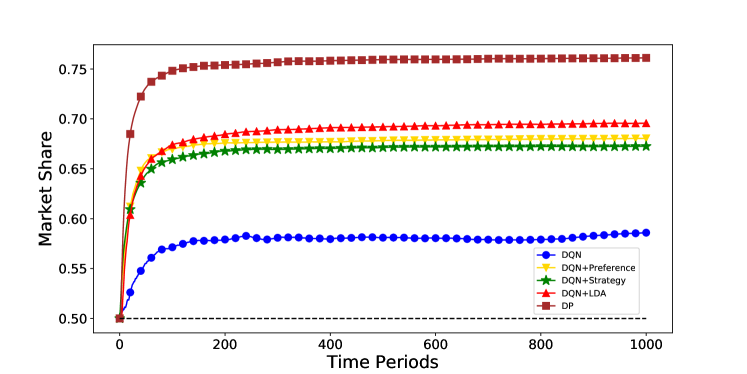
(a) Market share curves when playing against Random Strategy.

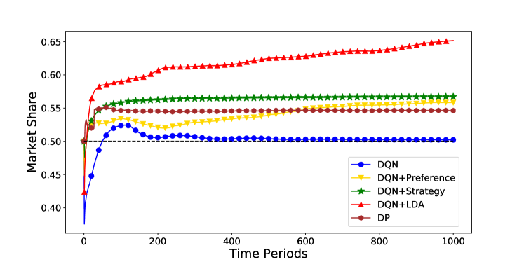
(b) Market share curves when playing against DQN.

Figure 4: Market share curves in simulation experiments.

And Fig.4 shows the average market share of company 1 after $t$ time periods, when using different strategies competing against company 2 using baseline methods. We can find that the convergence procedures in the Fig. 4 (a) is faster and more stable than the ones in the Fig. 4 (b). The reason is that Random Strategy can be considered as the static environment, while DQN is evolving along with the rounds. This is in line with the intuition.

5 Real-World Dataset Analysis

In the simulated experiments, the latent information inferred by our model has shown great help in finding strategies to earn more market share. And in this section, we apply our model on a real-world dataset and conduct a series of experiments, to prove that the model can indeed infer our desired latent information. We first introduce our open dataset, followed by our preprocessing methods. Then, we provide quantified evaluation results compared with the baselines and finally analyze the results of our method from different aspects.

5.1 Coupon Usage Data for O2O

Coupon Usage Data for O2O, referred to O2O Dataset in following description, is an open dataset from the Tianchi contest [1]. O2O represents ”online to offline”, while a typical example of ”O2O marketing” is that merchants in a shopping mall send coupons to potential customers through emails or short messages in their own APPs. Merchants want to attract customers to their offline shops and decide these personalized discount rate of coupons based on a large amount of users’ behavior and location information recorded by various APPs.

In our experiment, we make use of the offline training data from O2O Dataset, where the coupon promotion is conducted by 7737 retail stores from Jan. 1st 2016 to June 30th 2016. There are 1,048,575 records in total, among which there are 255,550 users receiving 9280 kinds of coupons. In precise, each record consists of identifications for a user, a merchant and a coupon (or ’null’ if no coupon was provided), distance between the merchant and the user, the discount rate of the coupon, the date when the coupon was sent and the date when the coupon was used (or ’null’ if it was never used). After basic data cleaning and statistics, we know that on average each user receives $1.986$ coupons, while on average each kind of coupons is sent to $37.637$ customers. Generally speaking, $7.12\%$ coupons are used.

5.2 Preprocess

Unlike the simulated data, it requires a preprocessing at first for our model to apply on the real-world data. According to our model, it requires data for users with similar preference in each group, called preference group. And in each group, the opponent may adopt different strategies to different people. Since in the practice, we know neither the preferences of the users nor the strategies of the opponents, we need to cluster the data twice. Now we introduce the main steps of our preprocessing in detail.

5.2.1 Agents

Firstly, we consider each merchant in O2O Dataset as an agent in such a competitive environment, providing coupons to attract customers. In practice, each merchant is only accessible to those records related itself. And since our LDA can help infer latent variables on behalf of one agent, we choose the merchant with id 3381 as the company 1 in our model, since it has the largest number of records in the dataset. Then all other merchants are considered together as its opponent, in other word, the company 2 in our model.

To be precise, there are 74823 records related to company 1, among them, 8 kinds of coupons are provided to 64152 users. Those coupons, according to their discount rate, can be divided into three groups, namely coupons of level low, middle and high (denoted by 1,2,3 respectively). Another reason why we do not maintain the original types of coupons is that the number of records about offering each kind of coupons varies a lot.

5.2.2 Preference Group Clustering

To determine users with similar preference distribution (denoted by $P$), we cluster them into 4 different groups based on features only related to the merchant and users themselves.

5.2.3 Strategy Group Clustering

As we introduced before, our model considers the opponent adopts a stable strategy distribution, (denoted by $S$), for each user. But in O2O Dataset, the number of records for each user is too small. Therefore, we cluster users in each preference group into 10 different subgroups based on features only related to themselves. These subgroups are called strategy group, and we assume the opponent adopts the same strategy distribution for users in each strategy group.

Input: Dataset $D$, company 1, number of preference group $N$, number of strategy group $M$

Output: The preference distribution $\{P_{1},\dots,P_{N}\}$, the strategy distribution $\{S_{1,1},\dots,S_{N,M}\}$

1 $PG_{1},\dots,PG_{N}\leftarrow$ Cluster the users in the $D$ according to their preference to company 1.

2 for $i\leftarrow 1\textnormal{{to}}N$ do

3       $SG_{i,1},\dots,SG_{i,M}\leftarrow$ Cluster the users in $PG_{i}$ according to the opponent’s strategies. $P_{i},S_{i,1},\dots,S_{i,M}\leftarrow LDA(\{SG_{i,1},\dots,SG_{i,M}\})$

Algorithm 2 Preprocess of Coupon Usage Data

5.3 Evalution

In this subsection, we apply our model on the dataset and evaluate it by measuring its behavior prediction and inferred strategy distribution, to show that our model is effective.

5.3.1 Behavior Prediction

We first train our model on the training dataset, then we use our model to predict the behaviors of users in the testing dataset. We evaluate our model on the measurement of negative log likelihood for prediction, compared with some baselines.

Mathematically, negative log likelihood is defined as

$$\mathcal{L}(\theta)=-\sum\limits_{i=1}^{N}log(p(y_{i}|\theta,x_{i}))$$

, where $\theta$ is the model we want to evaluate, $N$ is the number of samples, $x_{i}$ is the features and $y_{i}$ is the ground truth of sample $i$, $p(y_{i}|\theta,x_{i})$ is the output probability of $y_{i}$ from model $\theta$ when given $x_{i}$. The smaller the likelihood of prediction is, the better the corresponding model is. And in our experiments, $N=7284$ for our model, as well as all the baselines.

We consider 5 common the probabilistic prediction models as baselines:

• Naive bayesian (NB) [25]

• Logistic Regression (LR)

• Support Vector Machine (SVM) [22]

• Random Forest (RF) [17]

• Neural Network (NN) [15]

All the above baslines are implemented by sklearn [21]. And their input features are the same extracted features we using for LDA.

Table 2: Comparison of Negative Log Likelihood

Model	NB	LR	SVM	RF	NN	LDA
Result	494.93	580.26	1085.40	597.93	509.26	401.97

As shown in Tab.2, our model get the smallest negative log likelihood in prediction, meaning that it provides the best modeling for the real-world data.

5.3.2 Distance of Strategy Distributions

We also evaluate the distribution distance between our strategy distribution and the real strategy distribution. The real strategy distribution for each strategy group is calculated by the number of coupons that all other merchants in the whole dataset provide to users in the group. Similar to the preprocessing, these coupons are also divided into three groups as level low, middle and high according to their discount rate. We adopt the Wasserstein Distance [23] to measure the distance of two distribution, which is defined as

$$W_{1}(\vec{p},\vec{q})=\operatorname{inf}\limits_{\pi\in\Gamma(\vec{p},\vec{q})}\int_{\mathbb{R}\times\mathbb{R}}|x-y|\operatorname{d}\pi(x,y)$$

, where $\Gamma(\vec{p},\vec{q})$ denotes the collection of all joint distributions on $\mathbb{R}\times\mathbb{R}$ whose marginals are $\vec{p}$ and $\vec{q}$ on the first and second factors respectively.

We consider two distributions as our baselines.

• The overall distribution of received coupons. We count the total number of each kind of coupons that all other merchants in the whole dataset provide to all users of company 1 as the baseline distribution.

• Uniform distribution: $p=(\frac{1}{3},\frac{1}{3},\frac{1}{3})$, which is what a single merchant may assume for its opponent without knowing further information.

As shown in Tab.3, the distance between our inferred distribution and the real distribution is the closest.

Table 3: Comparison of Distribution Distance

Model	Uniform	Average	LDA
Result	0.18794	0.13105	0.12303

5.4 Analysis

Unlike the opponent’s strategy that we can calculate from the dataset, the true preference distributions of users are hard to know. Therefore we analyze the inferred distributions to show that they are reasonable to some extent.

Firstly, we show the visual results of our preference clustering in Fig. 5. The aim of preference clustering is to cluster the users with similar preference to one merchant. From Fig. 5, we can see clearly that the users with the same preference are clustered together.

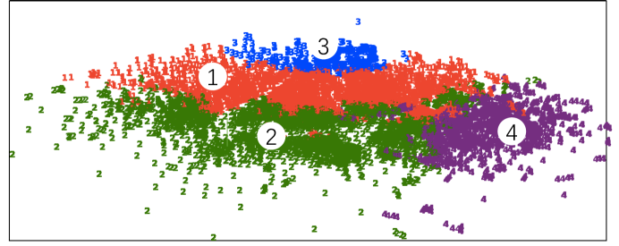
Figure 5: The visual results of our clustering for preference groups

Then, we show the preference distributions inferred by our model explicitly. Fig. LABEL:fig:pref_heatmap shows the heat-map of preference distributions of four clusters. The block ($i$, $j$) with lighter color represents when users receive ($i$, $j$) pair of coupons, the preference they choose company 1 is higher. ”Low”, ”Middle”, ”High” mean the effects of coupon respectively, as we introduced in Subsection. 5.2. We can find that when company 1 chooses high coupons, the preference distribution of users is very high, close to 100%. These results confirm our intuition.

We also plot the histogram of the distribution of preference in Fig.LABEL:fig:pref_hist. The histogram of preference distribution in each cluster. In each subfigure, the bars with the same colors mean that we adopt the same coupon. The ’Low’, ’Middle’, ’High’ in x-axis represent what coupons the opponent chooses respectively. The ’Infer Average’ represent the mean preference regardless of the opponent’s coupons when we choose the corresponding coupon. The ’Real Average’ represent the average usage rates of the coupons regardless of the opponent’s coupons when we choose the corresponding coupon. It is easy to see that when we choose the high effective coupon and the opponent choose the low effective coupon, the preference to us is very high. The most noticeable results in the Fig. LABEL:fig:pref_hist are the comparisons between ’Infer Avg’ and ’Real Avg’. We can find that if ’Real Avg’ is higher than other clusters, the ’Infer Avg’ is higher than other clusters too except the cluster 1, which is in line with the intuition.

6 Practical Financial Scenario

In this section, we present our experiments on real financial data in two aspects.

Dataset

We also evaluate our methods on the real business dataset from a company. The dataset is selected from its marketing records for its new service in September 2017, when coupons of different types were sent to customers to attract them to use the service. The dataset contains customers’ features (264 related attributes, such as one’s resident, age, gender and so on), types of their received coupons, and their response (whether they used the service) in the next 15 days. The ratios of the positive and negative samples is close 1 : 200.

Likelihood On Real Data

Similar to Section 5, we apply our model to this dataset, infer hidden variables from training data and make predictions on the testing data accordingly. We calculated its negative log-likelihood and compared it with those got from other baselines.

Table 4: Comparison of Likelihood

Model	NN	NB	LR	LDA
Result	449.52	701.56	1432.85	259.60

As shown in Table 4, 10000 records from the dataset are used, among which 90% is used for training and the rest for testing. The negative log likelihood of our method’s predictions on testing data is significantly smaller than other models, which means our method captures the users’ behaviors much better.

Practical Financial Marketing

With the help of the company, we tested our method on practical marketing for the same service. Similar to the process as the simulation experiments, we applied the DRL framework for Price War with the information learning from the Price War LDA (Fig. 3) to practical financial marketing. In December 2017, 600,000 customers of the company were divided randomly into three groups of the same size. Our framework decides awards for customers from one group, while Random Strategy and the standard DQN for other two respectively as baselines. Within two weeks after receiving awards, 2.8053% customers from the first group use the product, while 2.1697% of the second and 2.4966% of the third.

Compared with the usage rate of Random Strategy, our method got an improvement of 29.29% on usage rate, while DQN only got 15.07%. This means our method, considering opponent’s strategy and customer’s preference, do improve the effect of personalized marketing compared with those do not considering them.

7 Conclusions

In this paper, we formalize the Internet price war as an imperfect and incomplete information game. We design an LDA to explore unknown variables from one participant’s perspective. The inferred information is shown to help decision making method, like DRL and DP, for finding better strategies in simulated experiments. And the model also exhibits better characterization for an open dataset from a practical business. It is the first time that LDA is used in a game scenario and makes efforts in the competitive business environment. This design not only makes a major contribution towards achieving better market sharing in an Internet price war but also inspire a novel technique for dealing with incomplete and imperfect information games.

References

- [1] Aliyun.com. Coupon usage data for o2o. https://tianchi.alibabacloud.com/datalab/dataSet.html?dataId=59, 2018. [Online; accessed 31-May-2018].
- [2] David Besanko. The mother of all (pricing) battles: The 1992 airline price war. Kellogg School of Management Cases, pages 1–3, 2017.
- [3] David M Blei, Andrew Y Ng, and Michael I Jordan. Latent dirichlet allocation. Journal of machine Learning research, 3(Jan):993–1022, 2003.
- [4] Timothy F Bresnahan. Competition and collusion in the american automobile industry: The 1955 price war. The Journal of Industrial Economics, pages 457–482, 1987.
- [5] Wang Chong, David Blei, and Fei-Fei Li. Simultaneous image classification and annotation. In Computer Vision and Pattern Recognition, 2009. CVPR 2009. IEEE Conference on, pages 1903–1910. IEEE, 2009.
- [6] Liyan Chen Ellen Huet. World war uber: Why the ride-hailing giant can’t conquer the planet (yet). https://www.forbes.com, 2015.
- [7] Yuan Feng, Baochun Li, and Bo Li. Price competition in an oligopoly market with multiple iaas cloud providers. IEEE Transactions on Computers, 63(1):59–73, 2014.
- [8] RW Ferrero, JF Rivera, and SM Shahidehpour. Application of games with incomplete information for pricing electricity in deregulated power pools. IEEE Transactions on Power Systems, 13(1):184–189, 1998.
- [9] Ritwik Giri, Heesook Choi, Kevin Soo Hoo, and Bhaskar D Rao. User behavior modeling in a cellular network using latent dirichlet allocation. In International Conference on Intelligent Data Engineering and Automated Learning, pages 36–44. Springer, 2014.
- [10] He He, Jordan Boyd-Graber, Kevin Kwok, and Hal Daumé III. Opponent modeling in deep reinforcement learning. In International Conference on Machine Learning, pages 1804–1813, 2016.
- [11] Johannes Heinrich and David Silver. Deep reinforcement learning from self-play in imperfect-information games. arXiv preprint arXiv:1603.01121, 2016.
- [12] Yi-Chun Ho, Yi-Jen Ho, and Yong Tan. Online cash-back shopping: Implications for consumers and e-businesses. Information Systems Research, 28(2):250–264, 2017.
- [13] Andreas Krämer, Martin Jung, and Thomas Burgartz. A small step from price competition to price war: understanding causes, effects and possible countermeasures. International Business Research, 9(3):1, 2016.
- [14] Steffen L Lauritzen. Causal inference from graphical models. Complex stochastic systems, pages 63–107, 2001.
- [15] Yann LeCun, Yoshua Bengio, and Geoffrey Hinton. Deep learning. nature, 521(7553):436, 2015.
- [16] Huayu Li, Rongcheng Lin, Richang Hong, and Yong Ge. Generative models for mining latent aspects and their ratings from short reviews. In Data Mining (ICDM), 2015 IEEE International Conference on, pages 241–250. IEEE, 2015.
- [17] Andy Liaw, Matthew Wiener, et al. Classification and regression by randomforest. R news, 2(3):18–22, 2002.
- [18] Xin Luo, Mingsheng Shang, and Shuai Li. Efficient extraction of non-negative latent factors from high-dimensional and sparse matrices in industrial applications. In Data Mining (ICDM), 2016 IEEE 16th International Conference on, pages 311–319. IEEE, 2016.
- [19] Patrick Maillé and Bruno Tuffin. Price war in heterogeneous wireless networks. Computer Networks, 54(13):2281–2292, 2010.
- [20] Volodymyr Mnih, Koray Kavukcuoglu, David Silver, Andrei A Rusu, Joel Veness, Marc G Bellemare, Alex Graves, Martin Riedmiller, Andreas K Fidjeland, Georg Ostrovski, et al. Human-level control through deep reinforcement learning. Nature, 518(7540):529, 2015.
- [21] Fabian Pedregosa, Gaël Varoquaux, Alexandre Gramfort, Vincent Michel, Bertrand Thirion, Olivier Grisel, Mathieu Blondel, Peter Prettenhofer, Ron Weiss, Vincent Dubourg, et al. Scikit-learn: Machine learning in python. Journal of machine learning research, 12(Oct):2825–2830, 2011.
- [22] John Platt et al. Probabilistic outputs for support vector machines and comparisons to regularized likelihood methods. Advances in large margin classifiers, 10(3):61–74, 1999.
- [23] Aaditya Ramdas, Nicolás García Trillos, and Marco Cuturi. On wasserstein two-sample testing and related families of nonparametric tests. Entropy, 19(2):47, 2017.
- [24] Akshay R Rao, Mark E Bergen, and Scott Davis. How to fight a price war. Harvard Business Review, 78(2):107–120, 2000.
- [25] Irina Rish. An empirical study of the naive bayes classifier. In IJCAI 2001 workshop on empirical methods in artificial intelligence, volume 3, pages 41–46. IBM, 2001.
- [26] Jean-Charles Rochet and Jean Tirole. Platform competition in two-sided markets. Journal of the european economic association, 1(4):990–1029, 2003.
- [27] Rajiv Sethi and Eswaran Somanathan. Preference evolution and reciprocity. Journal of economic theory, 97(2):273–297, 2001.
- [28] Nicholas Shields. Uber’s losses grow in q3, but bookings rise. https://www.forbes.com, 2017.
- [29] Richard S Sutton and Andrew G Barto. Reinforcement learning: An introduction, volume 1. MIT press Cambridge, 1998.
- [30] Harald J Van Heerde, Els Gijsbrechts, and Koen Pauwels. Winners and losers in a major price war. Journal of Marketing Research, 45(5):499–518, 2008.
- [31] Shiying Wang, Huimiao Chen, and Desheng Wu. Regulating platform competition in two-sided markets under the o2o era. International Journal of Production Economics, 2017.
- [32] Junyu Xuan, Jie Lu, Guangquan Zhang, Richard Yi Da Xu, and Xiangfeng Luo. Infinite author topic model based on mixed gamma-negative binomial process. In Data Mining (ICDM), 2015 IEEE International Conference on, pages 489–498. IEEE, 2015.
- [33] Jun Yu, Sunil Mohan, Duangmanee Pew Putthividhya, and Weng-Keen Wong. Latent dirichlet allocation based diversified retrieval for e-commerce search. In Proceedings of the 7th ACM international conference on Web search and data mining, pages 463–472. ACM, 2014.