Ground-state properties of the one-dimensional transverse Ising model in a longitudinal magnetic field

Abstract

The critical properties of the one-dimensional spin-$1/2$ transverse Ising model in the presence of a longitudinal magnetic field were studied by the quantum fidelity method. We used exact diagonalization to obtain the ground-state energies and corresponding eigenvectors for lattice sizes up to 24 spins. The maximum of the fidelity susceptibility was used to locate the various phase boundaries present in the system. The type of dominant spin ordering for each phase was identified by examining the corresponding ground-state eigenvector. For a given antiferromagnetic nearest-neighbor interaction $J_{2}$, we calculated the fidelity susceptibility as a function of the transverse field $B_{x}$ and the longitudinal field $B_{z}$. The phase diagram in the ($B_{x},B_{z}$)-plane shows three phases. These findings are in contrast with the published literature that claims that the system has only two phases. For $B_{x}<1$, we observed an antiferromagnetic phase for small values of $B_{z}$ and a paramagnetic phase for large values of $B_{z}$. For $B_{x}>1$ and low $B_{z}$, we found a disordered phase that undergoes a second-order phase transition to a paramagnetic phase for large values of $B_{z}$.

I Introduction

There is an ongoing interest in the zero-temperature properties of quantum spin systems Sac11 ; Yus18 . In particular on the nature of phase transitions that occur due to the presence of pure quantum fluctuations since thermal fluctuations are absent. These transitions are triggered when a Hamiltonian parameter crosses a given value, upon which there occurs a change in the spin arrangement in the underlying lattice. Such transitions are regarded as second-order when the changes of the ground-state properties are continuous. On the other hand, if the changes are discontinuous the system undergoes a first-order transition. All of these can only occur at the thermodynamic limit, when the size of the system is infinite.

The one-dimensional (1D) transverse Ising model in a longitudinal field is a relatively simple model that displays both continuous and discontinuous transitions. Thus it has drawn a considerable amount of interest in the literature. Several approaches have been used to study that model, namely, entanglement measures Yus18 , simulations with ultra-cold atoms in optical lattices Sim11 ; Lew07 ; Blo08 ; Gre02 , density matrix renormalization group (DMRG) Ovc03 ; Cam14 ; Rob17 ; Pel18 , quantum Monte Carlo Nov86 , neural networks Czi18 , exact diagonalization Sen00 ; Ban11 , and finite size scaling Cam14 ; Ros18 . In numerical calculations, finite-size scaling is often employed to infer the location of the transitions in the thermodynamic limit.

In the present work, we use the fidelity method to find the zero-temperature phase diagram of the 1D spin-$1/2$ transverse Ising model in a longitudinal field. That method is well suited to the identification of phase changes, as it relies upon the detailed properties of the ground-state eigenvectors Ben92 ; Aba08 ; Coz07 ; Bon17 . It is very sensitive to changes in the quantum state of the system, and provides precise information about the location of the phase transitions as a given Hamiltonian parameter is varied. The nature of the transition can also be determined by the method. It has been used to detect and characterize a variety of phase transitions without requiring prior knowledge of the local order parameter of the system. This point of view also leads to new ways of looking at phase transitions and reveals the origin of their universalities.

Due to its simplicity and ability to locate phase transitions, quantum fidelity has been used in quantum information theory Ben92 and for the identification of topological phases in condensed matter physics Aba08 ; Coz07 . A unified approach connecting Berry phases and quantum fidelity has been established Ven07 . Monte Carlo schemes were introduced to compute the fidelity and its susceptibility for large interacting many-body systems in arbitrary dimensions Sch09 . An analysis of the transverse Ising model in the thermodynamic limit shows the universal properties of the fidelity near a critical point Ram11 .

The fidelity method has also been used to identify the universality class of the quantum transitions in the 1D asymmetric Hubbard model Gu08 . Scaling relations for the fidelity susceptibility in the quantum critical regime have been derived Alb10 . The scaling behavior of the fidelity susceptibility in the vicinity of a quantum multicritical point has been also studied Muk11 . The quantum properties of the two-dimensional version of the present model has been investigated by exact diagonalization using both longitudinal and transverse fidelity susceptibilities Nis13 . An exact expression for the fidelity susceptibility for the Ising model in a transverse field has been derived Dam13 . Quantum fidelity has been used to identify ground-state degeneracy of quantum spin systems Su13 . The behavior of the ground-state fidelity susceptibility in 1D quantum systems displaying a Berezinskii-Kosterlitz-Thouless type transition has been also investigated Sun15 . A method to calculate the fidelity susceptibility of correlated bosons, fermions and quantum spins systems at both zero and non-zero temperatures has been proposed using a variety of quantum Monte Carlo methods Wan15 . An extension and generalization of the application of the fidelity susceptibility to strongly correlated lattices systems has been put forward Hua16 . Closed-form expressions for the fidelity susceptibility of the anisotropic $XY$-model in a transverse field has been recently found Luo18 . Dynamical phase transitions at finite temperatures have recently been studied in topological systems by means of fidelity susceptibility Mer18 . A comprehensive review of the fidelity approach to quantum phase transitions is given in Ref. Gu10 .

Recently, the fidelity method was used to study the transverse Ising model with next-to-nearest neighbor interactions Bon17 , where it uncovered other quantum phases whose existence had been overlooked by other approaches. Thus, the fidelity method helped to uncover a much richer phase diagram for that model.

The phase diagrams found in the literature for the 1D spin-$1/2$ transverse Ising model in a longitudinal field show an antiferromagnetic phase at low fields and a paramagnetic phase at high fields Yus18 ; Sim11 ; Ovc03 . There appears a transition line for a continuous transition belonging to the same universality class of the 2D Ising model Sen00 . When the transverse field vanishes, the model shows a multicritical point where a first-order transition occurs. The phase diagrams in the literature show a single transition between antiferromagnetic and paramagnetic phases. As we shall see below, our fidelity approach uncovers an additional phase boundary line between the paramagnetic phase and a disordered phase, in addition to reproducing the boundary line found in the literature.

This paper is organized as follows: In Sec. II we present the model, while in Sec. III we discuss the fidelity susceptibility method. In Sec. IV we present our results and finally, we summarize our results in Sec. V.

II The Model

The 1D transverse Ising model in the presence of a longitudinal field is written as

$${\cal H}=J_{2}\sum_{i}\sigma^{z}_{i}\sigma^{z}_{i+1}-B_{x}\sum_{i}\sigma^{x}_{i}-B_{z}\sum_{i}\sigma^{z}_{i}.$$ (1)

The chain consists of $L$ spin-half interacting spins, written in terms of Pauli operators, where $\sigma^{\alpha}_{i}$ $(\alpha=x,y,z)$ is the $\alpha$-component located at site $i$. We consider a chain with periodic boundary conditions. The nearest-neighbor Ising coupling is antiferromagnetic, that is $J_{2}>0$, while the applied longitudinal field $B_{z}>0$ tends to align the spins ferromagnetically. For $B_{z}>0$ the model is gapped with a non-degenerate ground-state. Finally, quantum fluctuations are induced by a transverse magnetic field $B_{x}$. In what follows, we take $J_{2}=1$ as the energy unit.

When $B_{x}=0$, the Hamiltonian reduces to the Ising model in a longitudinal magnetic field. In that case the model shows a first-order phase transition at $B_{z}=2.0$. For $B_{x}\geq 0$, the ground state of the system in the low-field regime ($B_{z}<2.0$) is antiferromagnetic, whereas for high fields ($B_{z}>2.0$) it is paramagnetic separated by a second-order transition except at the multicritical point $(B_{x},B_{z})=(0.0,2.0)$ where the quantum fluctuations are suppressed and a classical first order phase transition occurs Sim11 .

On the on the hand, for $B_{z}=0$, the Hamiltonian becomes the transverse Ising model, whose ground-state properties were exactly obtained by Pfeuty in 1970 Pfe70 . He found that quantum fluctuations induced by the transverse field drive the system through a second-order phase transition at $B_{x}=1.0$. At low-fields the phase is antiferromagnetic, whereas for high fields it is disordered.

III The Fidelity Approach

Consider an Hamiltonian that depends on an arbitrary parameter $\lambda$, which drives the system through a phase transition when $\lambda=\lambda_{c}$. We define the quantum fidelity of a ground-state as the magnitude of the overlap between two neighboring ground-states, namely,

$$F(\lambda,\delta)=|\Braket{\psi(\lambda)}{\psi(\lambda+\delta)}|,$$ (2)

where $\Ket{\psi}$ is the normalized non-degenerate ground-state eigenvector evaluated near a given value of $\lambda$ by an arbitrary small shift $\delta$.

Quantum fidelity also depends on the system size. As the system approaches a quantum transition, the fidelity behavior changes dramatically. It drops from a level close to unity on either side of the transition point, to a minimum value at the transition point. This is caused by the distinct nature of the ground-state at each side of that transition point.

Instead of working with quantum fidelity as defined above, it is preferable to work with the fidelity susceptibility, which is obtained by expanding the fidelity as a Taylor’s series for very small $\delta$ about $\lambda$. Assuming that the ground state is normalized, the fidelity susceptibility can be written as

$$\chi(\lambda)=2(1-F(\lambda,\delta))/\delta^{2}+{\cal{O}}(\delta^{2}).$$ (3)

In the present work, the ground-state energy and eigenvector for a given $\lambda$ are found by using both Lanczos and conjugate gradient methods. The latter has been used in Hamiltonian models in statistical physics and transfer-matrix techniques  Nig90 ; Nig93 . For a given accuracy, both methods give the same results for the ground-state eigenvectors and energies.

Since the Hamiltonian (1) depends on two independent parameters, $B_{x}$ and $B_{z}$, we must investigate each of their associated susceptibilities. To differentiate between them, we use the notation $\chi_{\gamma}(\lambda)$, where $\lambda$ is chosen as one of the fields, and $\gamma$ is the other field, which is kept fixed during the calculations. In our numerical calculations, the boundary lines are found by using Eq. (3) with $\delta=0.001$ with a range of accuracy between $10^{-12}$ and $10^{-14}$ for the ground-state energy, depending on the chain size. For each $\lambda$, the location of the phase boundary is determined by the maximum of the fidelity susceptibility.

We write the Hamiltonian using the standard basis consisting of a tensor product of $L$ eigenstates of the $z$-component of the Pauli operator $\sigma^{z}_{i}$ located at site $i$, namely $|n>=\prod_{i}^{L}\,|s>_{i}$. On each site $i$ we have $s=0,1$, where $|s=1>_{i}$ denotes the eigenvector of $\sigma^{z}_{i}$ for an up-spin, and $|s=0>_{i}$ is the corresponding eigenvector for a down-spin. The index $n$ labels the basis states and has the values $n=0,1,...,N-1$, with $N=2^{L}$ which denotes the size of the Hilbert space.

By writing the basis index $n$ in binary notation, each of the $L$ binary digits will represent the z-component of the spin at a given site $i$ of a lattice with $L$ spins. An arbitrary eigenstate of the Hamiltonian can therefore be written as:

$$|\phi_{\alpha}>=\sum_{n=0}^{N-1}a_{\alpha}(n)|n>,$$ (4)

where the energy levels are labeled by $\alpha=0,1,...,N-1$. In particular, $\alpha=0$ is assigned to the ground-state.

Because of the symmetry of the Hamiltonian (1), the coefficients $a_{\alpha}(n)$ are real. The full wave vector can be visualized by plotting the amplitudes $a_{\alpha}(n)$ for any lattice size $L$, as a function of the state index $n$ in a single graph Bon06 ; Boe14 ; Bon14 .

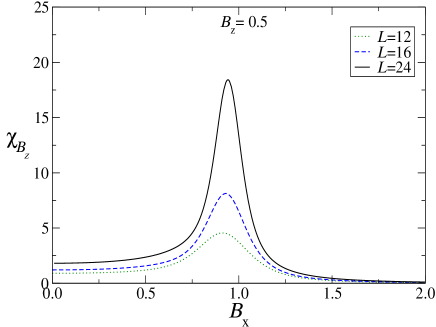
Figure 1: (color online) Fidelity susceptibility as a function of the transverse field $B_{x}$ for a fixed longitudinal field $B_{z}=0.5$, and lattice sizes $L=12$, $16$, and $24$. The maximum of the susceptibility specifies the location of the transition point. We set $J_{2}=1$ as the unity of energy for this and the subsequent figures.

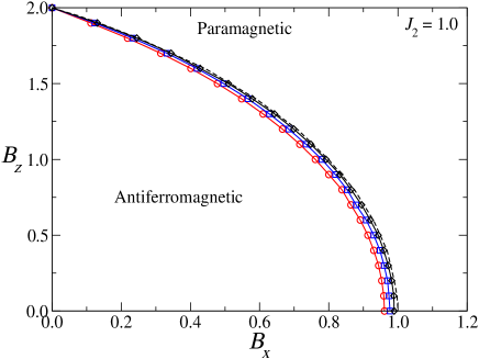
Figure 2: (color online) Phase diagram in the $(B_{x},B_{z})$-plane for chains sizes $L=12$ (circles), $16$ (squares) and $24$ (diamonds), obtained from the maximum of $\chi_{B_{z}}$. The model shows two phase regions, antiferromagnetic and paramagnetic. The transition points $(B_{x},B_{z})=(0,2)$ and $(B_{x},B_{z})=(1,0)$ are exact results. The dashed line is the critical line from DMRG results (Ref. Ovc03 ).

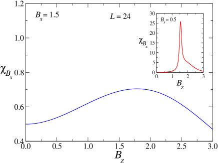
Figure 3: (color online) Fidelity susceptibility vs longitudinal field $B_{z}$ for a chain of size $L=24$, and fixed transverse fields $B_{x}$ = 1.5 and 0.5 (inset). The maximum of the susceptibility locates the transition point.

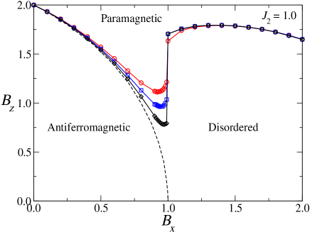
Figure 4: (color online) Phase diagram in the $(B_{x},B_{z})$-plane for chains with $L=12$ (circles), $16$ (squares), and $24$ (diamonds), obtained from the maxima of $\chi_{B_{x}}$. The model shows three phase regions, antiferromagnetic, paramagnetic, and disordered. The transition points at $(B_{x},B_{z})=(0,2)$ and $(B_{x},B_{z})=(1,0)$ are known exact results. The dashed line is the critical line from DMRG (Ref. Ovc03 ).

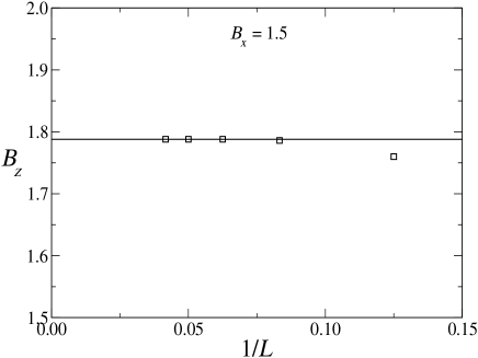
Figure 5: (color online) Critical value $B_{z}$ at the transition line between disordered and paramagnetic phases as a function of $1/L$ for $B_{x}=1.5$. The extrapolated straight line to the origin yields the thermodynamic value $B_{z}=1.788$.

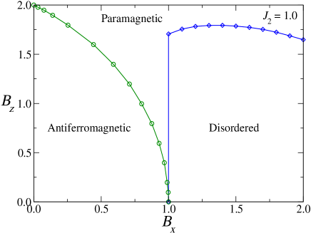
Figure 6: (color online) Full phase diagram of the model in the $(B_{x},B_{z})$-plane using the results of the present work (diamonds) and those of DMRG (open circles). The model shows three phase regions, antiferromagnetic, paramagnetic, and disordered. The transition points $(B_{x},B_{z})=(0,2)$ and $(B_{x},B_{z})=(1,0)$ are known exact results. These phases are separated by second-order phase transitions.

IV Results

In our numerical calculations we used even lattice sizes from $L$ = 8 to 24. This choice of lattice sizes preserves the symmetry of the ground state when the system is in the antiferromagnetic phase. In addition, it avoids undesirable frustration effects due to the finite size of the system and the imposed periodic boundary conditions.

To obtain the phase diagram of the model, we first calculated the fidelity susceptibility as a function of the transverse field $B_{x}$ for a fixed longitudinal field $B_{z}$. We represented this susceptibility as $\chi_{B_{z}}$. In Fig. 1 we show the behavior of $\chi_{B_{z}}$ for three lattice sizes $L=12$, $16$ and $24$, for the particular value of the longitudinal field $B_{z}=0.5$. In all calculations involving the susceptibility, we have used $\delta$= 0.001. The maximum of the susceptibility for each lattice size is taken as the quantum transition point from antiferromagnetic to paramagnetic phases for this particular value of longitudinal field.

By carrying out such calculations for different values of longitudinal fields in the interval $(0,2)$, we obtained the phase diagram shown in Fig. 2. The results for $L=12$ (open circles) , 16 (squares) and 24 (diamonds) are shown together with the critical boundary (dashed line) from Ovc03 calculated using DMRG. As one can see, by increasing the lattice sizes from $L=12$ to $24$ the critical line from the fidelity method gradually approaches the DMRG results. The critical line for $L$ = 24 is almost indistinguishable from that of DMRG. This is the full phase diagram of the model, as reported in the literature Ovc03 ; Sim11 ; Yus18 .

However, an analysis of the phase transitions for small longitudinal or transverses fields shows an inconsistency in the phase diagram of Fig. 2. For instance, for small transverse fields we expect an antiferromagnetic to paramagnetic phase transition boundary near $B_{z}=2$. On the other hand, in the limit of small longitudinal fields, and based on the exact results for the transverse Ising model, we expect an antiferromagnetic to disordered transition near $B_{x}=1$.

Another way to see this is that for low $B_{x}$ and high $B_{z}$, the spins should be pointing in the z-direction and for opposite case, namely low $B_{z}$ and high $B_{x}$, the spins should be pointing in the x-direction. Thus these two configurations cannot be part of the same phase. Therefore a phase boundary between the disordered-paramagnetic phase must be present in the phase diagram, Fig. 2.

We will show below that by evaluating a second fidelity susceptibility for a fixed transverse field ($\chi_{B_{x}}$) this missing phase boundary can be located. As in the case of Fig. 2, we first calculated the susceptibility $\chi_{B_{x}}$ as a function of $B_{z}$ for fixed values of $B_{x}$. Figure 3 shows the results for $B_{x}=1.5$ and $0.5$ (inset). The value $B_{x}$ = 0.5 lies within the antiferromagnetic phase, while $B_{x}$ = 1.5 is in the disordered phase.

A point worth noticing in Fig. 3 is the relatively high ratio between the two fidelity susceptibility maxima. The susceptibility maximum across the transition from the antiferromagnetic phase to the paramagnetic phase, shown in the inset, is about $35$ times larger than that of the maximum for the disordered to paramagnetic phase of the main figure. That is to be expected since the destruction of the antiferromagnetic order produces a very small fidelity (overlap of the wavefunctions) at the transition, hence a large susceptibility. On the other hand, the overlap between the disordered and the paramagnetic phases should be substantially larger, since no particular spin ordering is being broken, causing the susceptibility peak to be much less pronounced. Perhaps that is the reason why the disorder to paramagnetic transition has been overlooked in the treatments using other methods Ovc03 ; Sim11 ; Yus18 .

The phase diagram obtained using the maxima of $\chi_{B_{x}}$ for magnetic fields in the interval ($0\leq B_{z},B_{x}\leq 2$) for lattice sizes $L$ = 12, 16, and 24 is depicted in Fig. 4. For comparison, we have also included the DMRG results (dashed line). The transition boundary between the antiferromagnetic and paramagnetic phases gets closer to the DMRG results as the chain size increases (although the convergence is slower for the susceptibility $\chi_{B_{z}}$). Our fidelity results for the phase boundaries of different lattice sizes converge quite rapidly. The boundary between the disordered and paramagnetic phases for $L$ = 16 and $L$ = 24 are already indistinguishable in the scale of the figure. Figure 5 illustrates the convergence of results for the critical field $B_{z}$ as we consider larger lattices. In that figure, $B_{x}=1.5$. It shows the values of $B_{z}$ which maximize the susceptibility as a function of the inverse lattice size $1/L$. As can be seen, the data converges rapidly to $B_{z}=1.788$ at the thermodynamic limit. Thus, the two fidelity susceptibilities $\chi_{B_{x}}$ and $\chi_{B_{z}}$ complement each other in the determination of the phase boundaries. By combining the results of the present work and those of DMRG, we arrived at the full phase diagram for the model, depicted in Fig. 6.

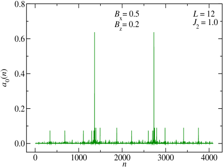
Figure 7: (color online) Ground-state amplitudes vs the basis state index $n$ for $(B_{x},B_{z})=(0.5,0.2)$, within the antiferromagnetic phase for $L=12$. The two largest amplitudes correspond to an antiferromagnetic ordering. The smaller amplitudes are a signature of the transverse magnetic field.

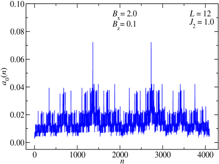
Figure 8: (color online) Ground-state amplitude vs basis state index $n$, for $(B_{x},B_{z})=(2.0,0.1)$, in the disordered phase for $L=12$. This spin configuration corresponds to a disordered phase. The two largest amplitudes are for antiferromagnetic ordering. The smaller, yet comparable, amplitudes arise from quantum effects of the transverse magnetic field.

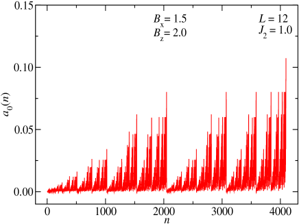
Figure 9: (color online) Ground-state amplitudes vs basis state index $n$ for $(B_{x},B_{z})=(1.5,2.0)$, within the paramagnetic phase for $L=12$. The largest amplitude corresponds to the ferromagnetic configuration.

The spin configuration of each phase can be found by plotting the ground-state eigenvector amplitudes as a function of the ground-state index $n$. As a working example we shall use $L$ = 12. For the point $(B_{x},B_{z})$= (0.5, 0.2) inside the antiferromagnetic phase, we obtained the plot depicted in Fig. 7. The two largest amplitudes are at $n$=1365 and $n$=2730, corresponding to a ground-state in the binary representation $|$010101010101$>$ and $|$101010101010$>$, respectively. The much smaller amplitudes are transverse field effects.

Moving to the disordered phase, we consider now the point $(B_{x},B_{z})=(2.0,0.1)$, where the ground-state amplitudes are shown in Fig. 8. Although the antiferromagnetic component is still present (due to the Ising interactions) as the larger component of the amplitudes, many other components with comparable amplitudes are also present.

Finally, we considered $(B_{x},B_{z})=(1.5,2.0)$, inside the paramagnetic phase. We obtained the graph shown in Fig. 9. The largest amplitude at $n=4096$ corresponds to the ferromagnetic configuration with all spins pointing in the direction of the field. The second largest amplitudes also correspond to a ferromagnetic configuration with all spins but one aligned with the field. The third largest amplitudes still correspond to a ferromagnetic configuration with all spins but two aligned with the field. Similar ferromagnetic configurations are found for the smaller amplitudes.

V Summary and Conclusions

The ground-state properties of the transverse Ising model in the presence of a longitudinal field was analyzed using the quantum fidelity method. The phase diagram in the $(B_{x},B_{z})$-plane shows three phases in contrast with previously reported results from the literature, which show only two phases. The phases are antiferromagnetic, paramagnetic, and disordered. These phases are separated by second-order phase transitions. We have also analyzed the spin configuration of the ground-state of each corresponding phase. The spins configuration on each phase clearly show distinct characteristics.

ACKNOWLEDGEMENTS

We thank C. Warner for critical reading of the manuscript. O.F.A.B. acknowledges support from the Murdoch College of Science Research Program and a grant from the Research Corporation through the Cottrell College Science Award No. CC5737. We also thank FAPERJ, CNPq and PROPPI (UFF) for financial support.

References

- (1) See, for example, S. Sachdev, Quantum Phase Transitions (Cambridge University Press, Cambridge, England, 2011).
- (2) A. Yuste, C. Cartwright, G. De Chiara, and A. Sanpera, New. J. Phys. 20, 043006 (2018).
- (3) J. Simon, W. S. Bakr, R. Ma, M. E. Tai, P. M. Preiss, and M. Greiner, Nature (London) 472, 307 (2011).
- (4) M. Lewenstein, et al., Adv. Phys. 56, 243 (2007).
- (5) I. Bloch, J. Dalibard, and W. Swerger, Rev. Mod. Phys. 80, 885 (2008).
- (6) M. Greiner, O. Mandel, E. Esslinger, T. W. Haensch, and I. Bloch, Nature 415 39 (2002).
- (7) A. A. Ovchinnikov, D. V. Dmitriev, V. Ya. Krivnov, V. O. Cheranovskii, Phys. Rev.B 68, 214406 (2003).
- (8) M. Campostrini, J. Nespolo, A. Pelissetto, and E. Vicari, Phys. Rev. Lett. 113, 070402 (2014).
- (9) B. Roberts, T. Vidick, and O. I. Motrunich, Phys. Rev. B 96, 214203 (2017).
- (10) A. Pelissetto, D. Rossini, and E. Vicari, Phys. Rev. E 98, 032124 (2018).
- (11) M. A. Novotny and D. P. Landau, J. Mag. Mag. Mat. 54, 885 (1986).
- (12) S. Czischek, M. Gärttner, and T. Gasenzer, Phys. Rev. B 98, 024311 (2018).
- (13) P. Sen, Phys. Rev. E 63, 016112 (2000).
- (14) M. C. Bañuls, J. I. Cirac, and M. B. Hastings, Phys. Rev. Lett. 106, 050405 (2011).
- (15) M. Campostrini, A. Pelissetto, and E. Vicari, Phys. Rev. 89, 094516 (2014).
- (16) D. Rossini, and E. Vicari, arXiv:1807.01674 (2018).
- (17) C. H. Bennett, G. Brassard, and N. D. Mermin, Phys. Rev. Lett. 68, 557 (1992).
- (18) D. F. Abasto, A. Hamma, and P. Zanardi, Phys. Rev. A 78, 010301 (2008).
- (19) M. Cozzini, P. Giorda, and P. Zanardi, Phys. Rev. B 75, 014439 (2007).
- (20) O. F. de Alcantara Bonfim, B. Boechat, and J. Florencio, Phys. Rev. E 96 042140 (2017).
- (21) L. C. Venuti, and P. Zanardi, Phys. Rev. Lett. 99, 095701 (2007).
- (22) D. Schwandt, F. Alet, and S. Capponi, Phys. Rev. Lett. 103,170501 (2009).
- (23) M. M. Rams, and B. Damski, Phys. Rev. Lett. 106, 055701 (2011).
- (24) S. Gu, H.-M. Kwok, W.-Q. Ning, and H.-Q. Lin, Phys. Rev. B 77, 245109 (2008).
- (25) A. F. Albuquerque, F. Alet, C. Sire, and S. Capponi, Phys. Rev. B 81, 064418 (2010).
- (26) V. Mukherjee, A. Polkovnikov, and A. Dutta, Phys. Rev. B 83, 075118 (2011).
- (27) Y. Nishiyama, Phys. Rev. E 88, 012129 (2013).
- (28) B. Damski, Phys. Rev. E 87, 052131 (2013).
- (29) Y. H. Su, B.-Q. Hu, S.-H. Li, and S. Y. Cho, Phys. Rev. E 88, 032110 (2013).
- (30) G. Sun, A. K. Kolezhuk, and T. Vekua, Phys. Rev. B 91, 014418 (2015).
- (31) L. Wang, Y.-H. Liu, J. Imriška, P. N. Ma, and M. Troyer, Phys. Rev. X 5, 031007 (2015).
- (32) L. Huang, Y. Wang, L. Wang, and P. Werner, Phys. Rev. B 94, 235110 (2016).
- (33) Q. Luo, J. Zhao, and X. Wang, Phys. Rev. E 98, 022106 (2018).
- (34) B. Mera, C. Vlachou, N. Paunković, V. R. Vieira, and O. Viyuela, Phys. Rev. B 97, 094110 (2018).
- (35) S. Gu, Int. J. Mod. Phys. B 24, 4371 (2010).
- (36) P. Pfeuty, Ann. Phys. (N.Y.) 57, 79 (1970).
- (37) M. P. Nightingale, in Finite-Size Scaling and Numerical Simulation of Statistical Systems, edited by V. Privman, World Scientific, Singapore, 1990.
- (38) M. P. Nightingale, V. S. Viswanath, and G. Müller, Phys. Rev. B 48, 7696 (1993).
- (39) O. F. de Alcantara Bonfim and J. Florencio, Phys. Rev. B 74, 134413 (2006).
- (40) B. Boechat, J. Florencio, A. Saguia, O. F. de Alcantara Bonfim, Phys. Rev. E 89, 032143 (2014).
- (41) O. F. de Alcantara Bonfim, A. Saguia, B. Boechat, J. Florencio, Phys. Rev. E 90, 032101 (2014).