Optimizing the tie-breaker regression discontinuity design

Abstract

Motivated by customer loyalty plans and scholarship programs, we study tie-breaker designs which are hybrids of randomized controlled trials (RCTs) and regression discontinuity designs (RDDs). We quantify the statistical efficiency of a tie-breaker design in which a proportion $\Delta$ of observed subjects are in the RCT. In a two line regression, statistical efficiency increases monotonically with $\Delta$, so efficiency is maximized by an RCT. We point to additional advantages of tie-breakers versus RDD: for a nonparametric regression the boundary bias is much less severe and for quadratic regression, the variance is greatly reduced. For a two line model we can quantify the short term value of the treatment allocation and this comparison favors smaller $\Delta$ with the RDD being best. We solve for the optimal tradeoff between these exploration and exploitation goals. The usual tie-breaker design applies an RCT on the middle $\Delta$ subjects as ranked by the assignment variable. We quantify the efficiency of other designs such as experimenting only in the second decile from the top. We also show that in some general parametric models a Monte Carlo evaluation can be replaced by matrix algebra.

1 Introduction

Airlines, hotels and other companies may offer incentives such as free upgrades to their most loyal customers. An e-commerce company may offer some analytic tools or other support to the customers most likely to benefit from them. A philanthropist may offer higher education scholarships to high school students with excellent GPAs. It is reasonable to expect some benefit from the subjects who receive the treatment, be it increased sales to a customer or better educational outcomes for a student. It is then of interest to measure the causal effect of these special treatments. A natural choice in this context is the regression discontinuity design (RDD) but that has the disadvantage of only estimating a causal impact right at the threshold point separating treated from untreated study subjects.

In this paper we study a tie-breaker design that can estimate the causal effect more broadly. That design injects some randomness into the decision near the cutoff. Our main contributions are to analyze the efficiency gains of tie-breaker designs versus RDD, and to study the tradeoffs behind deciding how much randomness to introduce. More randomness brings greater statistical efficiency, while at the same time, it is expected to reduce the value of the incentives by not applying them where they will be the most effective.

The RDD was originated by Thistlethwaite and Campbell (1960). In an RDD, subjects are sorted according to a treatment assignment variable $x$ and those for which $x$ exceeds a threshold $t$ get the treatment while others do not. Sometimes the assignment variable is called a running variable or a forcing variable. For background on RDD see Angrist and Pischke (2009, 2014), Imbens and Lemieux (2008), Jacob et al. (2012), Van Der Klaauw (2008), and Lee and Lemieux (2010).

Historically, regression discontinuity designs were fit by a regression including a polynomial in $x$ and a discontinuous predictor $1\{x>t\}$ whose coefficient was taken to be the estimated causal impact of the treatment at $x=t$. This approach is problematic. Low order polynomial estimates are biased by lack of fit, and high order ones are unstable (Gelman and Imbens, 2017). The more modern approach fits linear or quadratic or other low order local polynomial regression models to the left and right of the threshold using kernel weights proportional to $K(|x-t|/b)$ for a bandwidth $b>0$ and a kernel $K(\cdot)$ of bounded support. In the kernel regression approach, the estimated causal effect is the difference between those nonparametric regressions when extrapolated to $x=t$ using data sets on the left and the right of $t$. See Hahn et al. (2001) for a description, Porter (2003) for optimality results, and Calonico et al. (2014) for improved confidence interval estimation. Armstrong and Kolesár (2018) and Imbens and Wager (2019) optimize for regression functions in general convex classes while also taking special care with assignment variables that have a discrete distribution.

One problem with RDDs is that a causal estimate is only available at $x=t$. A randomized controlled trial (RCT) by contrast makes the treatment a random variable independent of $x$. An RCT would not be appropriate for a customer loyalty program, and even less so for a scholarship

This problem is well suited to a tie-breaker design. For an assignment variable $x$, subjects are assigned to a control condition if $x\leqslant A$, to a test condition if $x\geqslant B$ and their treatment (test or control) is randomized if $A<x<B$. If $A=B$, then no subjects are randomized and the design is an RDD. At the other extreme, if all the $x$ values are between $A$ and $B$, then the design is an RCT as described in texts on causal inference (Imbens and Rubin, 2015) or on experimental design (Box et al., 1978; Wu and Hamada, 2011). Tie-breaker designs are also called cutoff designs; see (Cappelleri and Trochim, 2003). If one is fitting kernel weighted regressions, then the tie-breaker design offers an additional advantage. Nonparametric regressions have their most severe bias problems at or outside the boundary of the observed data (Rice and Rosenblatt, 1983). When $A<B$ there is a whole interval of $x$ values for which the nonparametric regressions need not extrapolate.

Angrist et al. (2014) use a tie-breaker design to evaluate the effects of post secondary aid in Nebraska. In that setting, $x$ was a student ranking. Students were triaged into top, middle and bottom groups. The top students received aid, the bottom ones did not, and those in the middle group were randomized to receive aid or not. Aiken et al. (1998) report on a study about allocation of students to remedial English classes where the assignment variable is a measure of students’ reading ability before they matriculate.

Tie-breakers are not the only settings where the threshold varies. In fuzzy RDDs (Campbell, 1969) the threshold varies due to dependence on other variables that may be unavailable to the data analyst. The threshold can also vary in settings where subjects or others working on their behalf manipulate the value of $x$ in order to get the treatment (McCrary, 2008). Rosenman and Rajkumar (2019) propose a mitigation strategy. We focus on the tie-breaker setting because in our motivating problems the investigator has control of the treatment variable.

Our interest is in optimizing the size of the RCT within a tie-breaker experiment. For this purpose we need a statistical model. In Section 8 we give a very general approach to this problem but it provides no closed form results. For interpretable results, we work primarily with a model in which there are two linear regressions, one for treatment and one for control. This model was used by Goldberger (1972) and Jacob et al. (2012), who both find RCTs more efficient than RDDs, and we think it is the simplest one in which the tradeoff we study is interesting. We can interpolate between RCTs and RDDs using a quantity $\Delta\in[0,1]$ representing the fraction of experimental assignments, ranging from $\Delta=0$ for the RDD to $\Delta=1$ for the RCT. When the region of study is small then a linear model will perform similarly to the local linear models underlying kernel approaches to RDD. At the design stage we know a lot less about model goodness of fit than we will once the data are available and that is another reason to design with a simple working model.

Figure 1 illustrates tie-breaker designs for four values of $\Delta$. The assignment variable there has a Gaussian distribution, that we assume has been centered and scaled. The outcome variable is simulated from a linear model with a constant treatment effect. For instance, in the third panel, the top $1/6$ of subjects get the treatment, the bottom $1/6$ do not and a fraction $\Delta=2/3$ of the data in the middle have randomized allocation.

For a Gaussian assignment variable, the experimental region in the middle of the data is where the data are most densely packed, which may well be where we are most interested in learning the treatment effect. The effect of treatment appears to be more visually prominent at larger $\Delta$ in accordance with the greater statistical efficiency that we find here for larger $\Delta$.

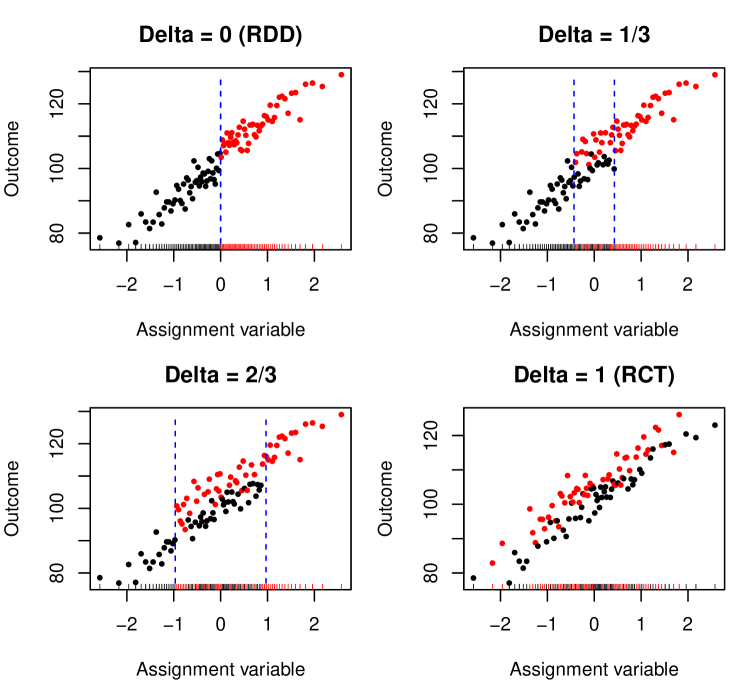
Figure 1: Illustrative data for tie-breaker designs with $\Delta\in\{0,1/3,2/3,1\}$, and a standardized Gaussian assignment variable. The regression discontinuity design has $\Delta=0$, the randomized controlled trial has $\Delta=1$. Treated points are plotted in red, control in black. Allocation is deterministic for $x$ outside the blue lines.

Our first working model is a two-line regression relating an outcome to a uniformly distributed assignment variable. The early sections of our paper work in this framework. Section 2 introduces that working model. The slope and intercept vary between treatment and control. Section 3 shows that the statistical efficiency of incorporating $\Delta>0$ experimentation versus the plain regression discontinuity design at $\Delta=0$ is ${1+3\Delta^{2}(2-\Delta^{2})}$, when $x\sim\mathcal{U}[-1,1]$. Thus, statistical efficiency is a monotone increasing function of the amount of experimentation. At the extreme, a pure RCT with $\Delta=1$ is $4$ times as efficient as the RDD as was found earlier by Jacob et al. (2012). We ordinarily expect that our outcome variable will show the greatest gains if we give the treatment to the highest ranked subjects and a tie-breaker design will then reduce those gains. Section 4 quantifies that cost in the two-line regression model and trades it off against statistical efficiency. The optimal $\Delta$ is then dependent on the ratio between the value per subject of the short term return and the value of the information per subject that we get for a given $\Delta$. It can be hard to know how much to weigh the information value compared to the short term value. A practical option is to choose the smallest $\Delta$ with at least a specified amount of efficiency with respect to the full experiment $\Delta=1$.

The later sections of our paper generalize beyond the working model. Section 5 repeats our analysis of the linear model for a pair of quadratic regression models. We see that the regression discontinuity design has a much higher variance than the experiment does, in line with the instability findings of Gelman and Imbens (2017) mentioned previously. An RCT can have orders of magnitude less variance than the RDD with tie-breaker designs in between. Section 6 handles the case of a Gaussian assignment variable that we illustrate in Figure 1. It is similar to the uniform case. Here a full RCT is $\pi/(\pi-2)\doteq 2.75$ times as efficient as the RDD as was found by Goldberger (1972).

Section 7 looks at replacing the three treatment probabilities $0$%, $50$% and $100$% by a strategy with more levels or even a continuous sliding scale $p(x)$ of the assignment variable $x$. We show that there is little to gain by this. If $p(x)$ satisfies $p(-x)=1-p(x)$, as with a symmetric CDF, then in a two line model both the information gained and the value from the experimental subjects in any sliding scale can also be attained by tie-breaker design using only levels $0\%$, $50\%$ and $100$%. A non-symmetric sliding scale can be symmetrized without affecting its cost and potentially reducing the variance of some of the regression coefficients. Using treatment probabilities $\epsilon$, $0.5$ and $1-\epsilon$ would not improve efficiency but would allow a potential outcomes analysis (Imbens and Rubin, 2015) of the data.

Section 8 describes a numerical version of our approach that does not require a simplistic regression model and allows users to choose their own. The design can then be chosen by an intensive numerical search with a Monte Carlo evaluation of each design choice. We show how to replace that simulation-based inner loop by matrix algebra allowing faster and more thorough optimization. We also find in Section 8 that experimenting on all data maximizes statistical efficiency in very general circumstances.

The tie-breaker literature has emphasized experiments in the middle range of the assignment variable $x$. Section 9 looks at off center experiments, such as experimenting in just the second decile from the top. In our motivating applications, the treatment might only be offered to a small fraction of subjects. Experimenting in the second decile reduces the most important regression coefficient’s variance to about 60% of what it would be with a comparably sized regression discontinuity design. When planning the experiment we don’t know whether the linear models that might work on the highest ranked subjects would hold for all subjects. At the time of analysis, we might opt to reduce a bias by only including the highest ranked 30% of subjects in the analysis. This is similar to a kernel weighting. Reducing the data set that way would greatly increase the variance of both the RDD and tie-breaker designs. Interestingly, in this example, the efficiency ratio between the two approaches is almost unchanged. Section 10 contains a short discussion of how to use the findings.

We close this introduction with an historical note. In the Lanarkshire milk experiment, described by Student (1931) the goal was to measure the effect of a daily ration of milk on the health of school children. Among many complications was the fact that some of the schools chose to give the rations to the students that they thought needed it most. While that may have been the most beneficial way to allocate the school’s milk, it was very damaging to the process of learning the causal impact of the milk rations. A tie-breaker experiment might have been a good compromise.

2 Setup

We begin with a simple setting where there are an even number $N$ of subjects $i=1,\dots,N$, and exactly $N/2$ of them will receive the treatment. There is an assignment variable $x_{i}\in\mathbb{R}$ for which it is reasonable to give the treatment to subjects with the largest values. The assignment variable might be the output of a statistical machine learning model based on multiple variables, or it could be based on a subjective judgment of one or more experts or stakeholders.

We will simplify the problem by transforming $x_{i}$ to be equispaced in the interval $[-1,1]$. That is, after sorting the subjects into increasing order of $x_{i}$, we make a rank transformation to $x_{i}=(2i-N-1)/N$. Let $z_{i}$ indicate the treatment status; subjects that receive the treatment have $z_{i}=+1$ and subjects that do not receive the treatment have $z_{i}=-1$.

We denote the experimental interval by $(-\Delta,+\Delta)$ for $\Delta$ in $[0,1]$. In our hybrid design the treatment assignment $z_{i}\in\{-1,1\}$ includes some randomization as follows:

$$\Pr(z_{i}=1\!\mid\!x_{i})=\begin{cases}\,\ \ 1,&x_{i}\geqslant\Delta\\ 1/2,&|x_{i}|<\Delta\\ \,\,-1,&x_{i}\leqslant-\Delta.\end{cases}$$ (1)

If $\Delta=0$, then we have a classic RDD with the discontinuity at $x=0$. If $\Delta=1$, then we have a classic RCT. If $0<\Delta<1$, then we have a tie-breaker design with $\Delta$ measuring the amount of randomization.

The random allocation in equation (1) will, on average, make half of the $z_{i}$ for $|x_{i}|<\Delta$ equal $1$ and the other half equal $-1$. One way to do this is to choose $z_{i}=1$ for a simple random sample of half of the elements in $R=\{i\mid|x_{i}|<\Delta\}$. Stratified schemes, setting $z_{i}=1$ for exactly one random member of each consecutive pair of indices in $R$ are also easy to implement.

The impact of the treatment is measured by a scalar outcome $Y$ where $Y_{i}$ is a measure of the benefit derived from subject $i$. That could be future sales in a commercial setting or a measure of post-secondary educational success for a scholarship. We suppose that the delay time between setting $z_{i}$ and observing $Y_{i}$ is long enough to make bandit methods (see for instance, Scott (2015)) unsuitable. We will instead compare experimental designs using the following two-line regression model:

$$Y_{i}=\beta_{0}+\beta_{1}x_{i}+\beta_{2}z_{i}+\beta_{3}x_{i}z_{i}+\varepsilon_{i},$$ (2)

where $\varepsilon_{i}$ are IID random variables with mean $0$ and finite variance $\sigma^{2}>0$. Our analysis is based on the regression model (2) instead of the randomization because the treatment for subjects with $x$ outside $(-\Delta,\Delta)$ is not random. See Section 7 for an alternative.

The effect of the treatment averaged over subjects $i=1,\dots,N$ is $2\beta_{2}$. The factor of $2$ comes from comparing $z_{i}=1$ to $z_{i}=-1$. We can also estimate whether the effect increases or decreases with $x$, through the coefficient $\beta_{3}$. The quantity $2\beta_{2}$ is also the magnitude of the treatment effect on a (hypothetical) average subject with $x=0$.

Under model (2), we can distinguish subjects for whom the treatment is effective from those for whom it is not. Suppose that $\tau$ is the incremental cost of offering the treatment to one subject. This might be a support cost or foregone revenue; in an educational context it would be the cost of offering a scholarship. If $\beta_{3}>0$, then there is a cutpoint

$$x_{*}=\frac{\tau-2\beta_{2}}{2\beta_{3}}$$

with $\mathbb{E}(Y\!\mid\!z=1)-\mathbb{E}(Y\!\mid\!z=-1)\geqslant\tau$ for subjects with $x\geqslant x_{*}$. If $x_{*}>1$ then the treatment does not pay off for any subject while if $x_{*}<1$ then it pays for all subjects. If $\beta_{3}<0$, then the treatment only pays off for subjects with $x_{i}\leqslant x_{*}$. We discuss that case further in Section 4.

3 Efficiency in the two-line model

We will analyze the data $(x_{i},Y_{i})$ for $i=1,\dots,N$ by fitting model (2) by least squares. The parameter of interest is $\beta=(\beta_{0},\beta_{1},\beta_{2},\beta_{3})^{\mathsf{T}}$ and we assume that $Y_{i}$ are independent random variables with $\mathrm{Var}(Y_{i})=\sigma^{2}$. The design matrix is $\mathcal{X}\in\mathbb{R}^{N\times 4}$ with $i$’th row $(1,x_{i},z_{i},x_{i}z_{i})$, and $\mathrm{Var}(\hat{\beta})=(\mathcal{X}^{\mathsf{T}}\mathcal{X})^{-1}\sigma^{2}$. Because $\sigma^{2}$ does not depend on $\Delta$, we can compare designs assuming that $\sigma=1$.

Next, we look at how $\mathcal{X}^{\mathsf{T}}\mathcal{X}$ depends on $\Delta$. For large $N$ we can replace $\sum_{i}x_{i}^{2}$ by $N\int_{-1}^{1}x^{2}\,\mathrm{d}x/2=N/3$. Similar integral approximations yield

$$\frac{1}{N}\mathcal{X}^{\mathsf{T}}\mathcal{X}\approx\begin{pmatrix}1&0&0&\phi(\Delta)\\ 0&1/3&\phi(\Delta)&0\\ 0&\phi(\Delta)&1&0\\ \phi(\Delta)&0&0&1/3\end{pmatrix},$$ (3)

where $\phi(\Delta)$ is the average value of $z\times x$ over the design. We let

$$z(x)=\mathbb{E}(z\!\mid\!x)=\begin{cases}-1,&x\leqslant-\Delta\\ \phantom{-}0,&|x|<\Delta\\ \phantom{-}1,&x\geqslant\Delta\end{cases}$$

and find that

$$\phi(\Delta)=\frac{1}{2}\int_{-1}^{1}xz(x)\,\mathrm{d}x=\frac{1}{2}\int_{-1}^{-\Delta}(-x)\,\mathrm{d}x+\frac{1}{2}\int_{\Delta}^{1}x\,\mathrm{d}x=\frac{1-\Delta^{2}}{2}.$$ (4)

The approximation error in (3) is $O_{p}(1/\sqrt{N})$ when the random $z_{i}$ are assigned by simple random sampling and it is much smaller under stratified sampling. We will work with (3) as if it were exact.

We can reorder the rows and columns of (3) to make it block diagonal,

$$\bordermatrix{&1&zx&z&x\cr\,1&1&\phi&0&0\cr zx&\phi&1/3&0&0\cr\,z&0&0&1&\phi\cr\,x&0&0&\phi&1/3\cr}$$

where the labels on the matrix above refer to the variables that the $\beta_{j}$ multiply and $\phi=\phi(\Delta)$. It follows that

$$N\times\mathrm{Var}\left(\begin{pmatrix}\hat{\beta}_{0}\\ \hat{\beta}_{3}\\ \hat{\beta}_{2}\\ \hat{\beta}_{1}\end{pmatrix}\right)=\frac{1}{1/3-\phi^{2}}\begin{pmatrix}1/3&-\phi&0&0\\ -\phi&1&0&0\\ 0&0&1/3&-\phi\\ 0&0&-\phi&1\\ \end{pmatrix}.$$ (5)

The individual coefficients’ variances are $\mathrm{Var}(\hat{\beta}_{0})=\mathrm{Var}(\hat{\beta}_{2})=1/(1-3\phi^{2})$ and $\mathrm{Var}(\hat{\beta}_{1})=\mathrm{Var}(\hat{\beta}_{3})=3/(1-3\phi^{2})$. These variances are smallest for small values of $\phi$, corresponding to large values of $\Delta$. That is, the more randomized experimentation there is in the data, the less variance there is in the estimates. Therefore, the RDD is least efficient and the RCT is most efficient. Larger values of $\phi$ also induce stronger correlations among the $\hat{\beta}_{j}$.

The estimated gain from the intervention for a subject with a given $x$ is $\hat{\mathbb{E}}(Y\!\mid\!x,z=1)-\hat{\mathbb{E}}(Y\!\mid\!x,z=-1)=2(\hat{\beta}_{2}+x\hat{\beta}_{3})$. Next

$$\mathrm{Var}(2(\hat{\beta}_{2}+x\hat{\beta}_{3}))=4\times\frac{1/3+x^{2}}{1/3-\phi^{2}}=\frac{16(1+3x^{2})}{1+3\Delta^{2}(2-\Delta^{2})}$$ (6)

after some algebra. The relative efficiency of the experiment versus regression discontinuity is

$$\frac{\mathrm{Var}\bigl{(}2(\hat{\beta}_{2}+x\hat{\beta}_{3});\Delta=0\bigr{)}}{\mathrm{Var}\bigl{(}2(\hat{\beta}_{2}+x\hat{\beta}_{3});\Delta=1\bigr{)}}=\frac{1+3(2-1)}{1+3\times 0}=4$$ (7)

for all $x$. That is, the randomized experiment with $N/4$ observations is as informative as the regression discontinuity with $N$ observations and this holds uniformly over all levels of the assignment variable $x$. This is the factor of $4$ from Jacob et al. (2012) mentioned earlier.

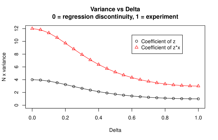
Figure 2: The top curve is the limiting value of $N\mathrm{Var}(\hat{\beta}_{3})$ plotted versus the fraction $\Delta$ of experimental data in the hybrid. Here $\beta_{3}$ is the regression coefficient of $xz$. The bottom curve corresponds to $N\mathrm{Var}(\hat{\beta}_{2})$ where $\beta_{2}$ is the coefficient of $z$.

Method	$\Delta$	$\mathrm{Var}(\hat{\beta}_{2})$	$\mathrm{Var}(\hat{\beta}_{3})$
Regression discontinuity	$0$	$4/N$	$12/N$
Experiment	$1$	$1/N$	$3/N$

Table 1: Variance of $\hat{\beta}_{2}$ (treatment effect intercept) and $\hat{\beta}_{3}$ (treatment effect slope) under regression discontinuity ($\Delta=0$) and randomized experiment ($\Delta=1$). It assumes that $\mathrm{Var}(Y\!\mid\!x,z)=1$.

Figure 2 shows the variance of the treatment effect parameters as a function of $\Delta$. Some values from the plot are shown in Table 1. The regression discontinuity design has four times the variance of the experiment as we saw in equation (7). The slope coefficient for treatment always has three times the variance of the intercept coefficient as follows from (5). Figure 3 show the variance of the estimated impact versus $x$ for several choices of $\Delta$.

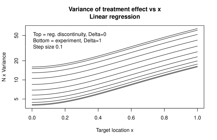
Figure 3: Variance of $2(\hat{\beta}_{2}+x\hat{\beta}_{3})$ versus $x$ in the two-line model (2), for $\Delta$ between $0$ and $1$ in steps of $0.1$. Note that the vertical axis is logarithmic.

4 Cost of experimentation

We ordinarily expect the value of the treatment to increase with the variable $x$. In that case the greatest return on the $N$ subjects in the experiment arises from the regression discontinuity design with $\Delta=0$. The information gain from $\Delta>0$ comes at some cost in the present sample. This section quantifies that cost.

For a deterministic allocation of $z=1$ or $z=-1$ we have $\mathbb{E}(Y\!\mid\!x,z)=\beta_{0}+\beta_{1}x+\beta_{2}z+\beta_{3}zx.$ When $z$ is chosen randomly with $\Pr(z=1)=\Pr(z=-1)=1/2$, then $\mathbb{E}(Y\!\mid\!x)=\beta_{0}+\beta_{1}x.$ It follows that the expected gain per subject in the hybrid design is

$$g(\Delta)=\mathbb{E}(Y) \equiv\frac{1}{2}\int_{-1}^{-\Delta}(\beta_{0}+\beta_{1}x-\beta_{2}-\beta_{3}x)\,\mathrm{d}x+\frac{1}{2}\int_{-\Delta}^{\Delta}(\beta_{0}+\beta_{1}x)\,\mathrm{d}x$$

$$\quad+\frac{1}{2}\int_{\Delta}^{1}\beta_{0}+\beta_{1}x+\beta_{2}+\beta_{3}x\,\mathrm{d}x$$

$$=\beta_{0}+\beta_{3}(1-\Delta^{2})/2.$$

Neither $\beta_{1}$ nor $\beta_{2}$ appear in this gain and the value of $\beta_{0}$ does not affect our choice of $\Delta$. Only $\beta_{3}$ which models how the payoff from the incentive varies with the assignment variable $x$ makes a difference. Compared to the regression discontinuity design with $\Delta=0$, the cost of incorporating experimentation is

$$N(g(0)-g(\Delta))=\frac{N\beta_{3}\Delta^{2}}{2},$$

which grows slowly as $\Delta$ increases from zero and then rapidly as $\Delta$ approaches one. If $\beta_{3}>0$, then as expected, we gain the most from the regression discontinuity design and the least from the experiment. This is a classic exploration-exploitation tradeoff.

It is possible that some settings have $\beta_{3}<0$. This might happen if the incentive is additional free tutoring in the educational context and the strongest students don’t need it, or if it is advice on how to best use an e-commerce company’s products in a context where higher performing customers already knew about the advice. In these cases the greatest gain comes from giving the incentive to the bottom $N/2$ customers and not the top $N/2$ customers. The analysis of this paper goes through by reversing the customer ranking, thereby replacing $x$ by $-x$ and also changing the sign of $\beta_{3}$.

Now we turn to optimizing the choice of $\Delta$ given some assumptions on the relative value of the information in the data for future decisions and the expected gain on the experiment. The precision (inverse variance) of our estimate of $\hat{\beta}$ is a linear function of $N$ and so is the expected gain. We can therefore trade off precision per subject with gain per subject. We think that $\beta_{3}$ is the most important parameter so we take the precision gain per subject to be

$$\mathrm{pre}(\Delta)\equiv\frac{1}{N\mathrm{Var}(\hat{\beta}_{3})}=\frac{1}{3}-\phi^{2}=\frac{1}{3}-\frac{(1-\Delta^{2})^{2}}{4}.$$ (8)

Alternatively, we could focus on $2\beta_{2}$ which is both the average gain per subject and the gain for a subject at $x=0$. The precision for $2\beta_{2}$ turns out to be $(3/4)\mathrm{pre}(\Delta)$ so it is perfectly aligned with precision on $\beta_{3}$. More generally, the gain from the incentive at any specific $x$ has a variance given by (6). Any weighted average of precision of $2(\beta_{2}+\beta_{3}x)$ over points $x\in[-1,1]$ is a scalar multiple of $\mathrm{pre}(\Delta)$ from (8).

We trade off gain per subject and precision per subject with the value function

$$\begin{split}v(\Delta)&=g(\Delta)+\lambda\cdot\mathrm{pre}(\Delta)=\beta_{0}+\beta_{3}\frac{1-\Delta^{2}}{2}+\lambda\Bigl{(}\frac{1}{3}-\frac{(1-\Delta^{2})^{2}}{4}\Bigr{)},\end{split}$$ (9)

where $\lambda>0$ measures the value for future decisions of having greater precision on $\beta_{3}$. Because $\lambda$ is about information gain for the future we consider it to have ‘long term’ value while $\beta_{3}$ describes value in the immediate data set, a relatively ‘short term’ consideration.

Proposition 1.

Let $v(\Delta)$ be given by equation (9) with $\lambda>0$ and $\beta_{3}\geqslant 0$. Then the maximum of $v$ over $\Delta\in[0,1]$ occurs at

$$\Delta_{*}=\begin{cases}1,&\phantom{0\leqslant}\beta_{3}/\lambda\leqslant 0\\ \sqrt{1-\beta_{3}/\lambda},&0\leqslant\beta_{3}/\lambda\leqslant 1\\ 0,&1\leqslant\beta_{3}/\lambda.\\ \end{cases}$$ (10)

Proof.

Let $\gamma=\Delta^{2}$. We will first maximize $v=c-\beta_{3}\gamma/2-\lambda(1-\gamma)^{2}/4$ over $0\leqslant\gamma\leqslant 1$, where $c$ does not depend on $\gamma$. Now $v$ has a unique maximum over $\gamma\in\mathbb{R}$ at $\gamma_{*}=1-\beta_{3}/\lambda$. The maximizing $\gamma$ is $\gamma_{*}$ when $0\leqslant\gamma_{*}\leqslant 1$, it is $0$ when $\gamma_{*}<0$ and it is $1$ when $\gamma_{*}>1$. Equation (10) translates these results back to the optimal $\Delta$. ∎

We see from equation (10) that the decision depends on the critical ratio $\beta_{3}/\lambda$. The numerator reflects the value of more efficient allocation and the denominator captures the value of improved information gathering. When $\beta_{3}\geqslant\lambda$ then the RDD with $\Delta=0$ is optimal. The full experiment, $\Delta=1$, is never optimal unless $\beta_{3}=0$ or the value $\lambda$ of information to be used in future decisions is infinite.

Figure 4: The horizontal axis has $\beta_{3}/\lambda$ where $\beta_{3}$ affects immediate gain per subject of the treatment allocation and $\lambda$ quantifies the value of precise slope estimation. The vertical axis gives the optimal $\Delta$ in a tie-breaker experiment.

Figure 4 shows the value $\Delta_{*}$ from equation (10) versus the ratio $r=\beta_{3}/\lambda$ of the short term to long term value coefficients. The function is nearly equal to $1-r/2$ near the origin and has negative curvature on $0\leqslant r\leqslant 1$. If future uses are important enough that $r\leqslant 1/10$, then one should use $\Delta\geqslant 1-0.1/2=0.95$. That is, when the future is very important the optimal hybrid is very close to an RCT.

In practice it may well be difficult to choose $\Delta$ to maximize the value (9) because we don’t know what $\lambda$ to choose and because the tradeoff depends on $\beta_{3}$ about which we may have little prior knowledge. The parameter $\lambda$ will be hard to choose because it quantifies the relative value of future information versus the present value of the intervention. A practical approach is to use the smallest experiment with at least some given proportion $\rho$ of the information available from the RCT. That is, for some $\rho\in[1/4,1]$, choose the smallest $\Delta$ with $\mathrm{pre}(\Delta)\geqslant\rho\times\mathrm{pre}(1)$. We don’t need to consider $\rho<1/4$ because even $\Delta=0$ has at least one fourth the efficiency of the RCT.

5 Quadratic regression

A quadratic regression model of the form

$$\mathbb{E}(Y)=\beta_{0}+\beta_{1}x+\beta_{2}z+\beta_{3}xz+\beta_{4}x^{2}+\beta_{5}x^{2}z$$ (11)

allows a richer exploration of the treatment effect. For instance, model (11) allows for the possibility that the treatment pays off if and only if $x$ is in some interval. It also allows for a situation where the payoff only comes outside of some interval. This model has even (symmetric) predictors $1$, $xz$, $x^{2}$ and odd (antisymmetric) predictors $x$, $z$, $zx^{2}$. As in the linear case, the even and odd predictors are orthogonal to each other.

Now $(1/N)\mathcal{X}^{\mathsf{T}}\mathcal{X}$ is a $6\times 6$ block diagonal matrix. Some of the entries are

$$\phi_{3}\equiv\phi_{3}(\Delta)=\frac{1}{2}\int_{-1}^{1}\mathbb{E}(z\!\mid\!x)x^{3}\,\mathrm{d}x=\int_{\Delta}^{1}x^{3}\,\mathrm{d}x=\frac{1-\Delta^{4}}{4}$$

as well as $\phi(\Delta)$ from Section 3 that we call $\phi_{1}(\Delta)$ here. We find that

$$\frac{1}{N}\mathcal{X}^{\mathsf{T}}\mathcal{X}=\bordermatrix{&1&zx&x^{2}&z&x&zx^{2}\cr\,1&1&\phi_{1}&1/3&0&0&0\cr zx&\phi_{1}&1/3&\phi_{3}&0&0&0\cr\,x^{2}&1/3&\phi_{3}&1/5&0&0&0\cr\,z&0&0&0&1&\phi_{1}&1/3\cr\,x&0&0&0&\phi_{1}&1/3&\phi_{3}\cr\,zx^{2}&0&0&0&1/3&\phi_{3}&1/5\cr}$$ (12)

after ignoring sampling or stratified sampling fluctuations. Once again we get a block diagonal pattern with two identical blocks. This is a consequence of $z^{2}=1$, and it will happen for more general models with odd and even predictors.

Proposition 2.

For $N>0$, let $\mathcal{X}^{\mathsf{T}}\mathcal{X}$ be given by (12). Then

$$(\mathcal{X}^{\mathsf{T}}\mathcal{X})^{-1}=\frac{1}{ND(\Delta)}\begin{pmatrix}M(\Delta)&0\\ 0&M(\Delta)\end{pmatrix}$$ (13)

for a $3\times 3$ symmetric matrix

$$M(\Delta)=\begin{pmatrix}\dfrac{1}{15}-\phi_{3}^{2}&\dfrac{\phi_{3}}{3}-\dfrac{\phi_{1}}{5}&\phi_{3}\phi_{1}-\dfrac{1}{9}\\[8.61108pt] {}^{\prime\prime}&\dfrac{4}{45}&\dfrac{\phi_{1}}{3}-\phi_{3}\\[8.61108pt] {}^{\prime\prime}&{}^{\prime\prime}&\dfrac{1}{3}-\phi_{1}^{2}\end{pmatrix},$$

and a determinant $D(\Delta)=4/{135}-{\phi_{1}^{2}}/5-\phi_{3}^{2}+(2/3)\phi_{1}\phi_{3}.$

Proof.

Multiplying $M(\Delta)$ above by the upper left $3\times 3$ submatrix in (12) yields $I_{3}$ times $D(\Delta)$, after some lengthy manipulations. ∎

Figure 5 show the variance of the estimated impact versus $x$ for several choices of $\Delta$. Notice that the variance is given on a logarithmic scale there. The regression discontinuity design $\Delta=0$ in the top curve there, has extremely large variances especially where $|x|$ is close to $1$. The randomized design at the bottom has much smaller variance. Even the maximum variance in the RCT (at $x=1$) is smaller than the minimum variance in the RDD (at $x=0$).

Figure 5: Variance of $2(\hat{\beta}_{2}+x\hat{\beta}_{3}+x^{2}\hat{\beta}_{5})$ versus $x$ in the quadratic model (11), for $\Delta$ between $0$ and $1$ in steps of $0.1$.

6 Gaussian case

In some settings, the original assignment variable $x$ might have a nearly Gaussian distribution. By changing location and scale we can suppose that $x$ has approximately the $\mathcal{N}(0,1)$ distribution, without loss of generality. We use $\varphi(\cdot)$ and $\Phi(\cdot)$ to represent the $\mathcal{N}(0,1)$ probability density function and cumulative distribution function, respectively.

We will experiment on the central data with $|x_{i}|\leqslant\tau$ choosing $\tau$ to get a fraction $\Delta$ of data in the experiment. That leads to $\tau=\Phi^{-1}((1+\Delta)/2)$. After reordering the variables we find in this case that

$$\frac{1}{N}\mathcal{X}^{\mathsf{T}}\mathcal{X}\approx\bordermatrix{&1&zx&z&x\cr\,1&1&\phi_{G}&0&0\cr zx&\phi_{G}&1&0&0\cr\,z&0&0&1&\phi_{G}\cr\,x&0&0&\phi_{G}&1\cr}.$$

The value of $\phi$ from the uniform case changes to

$$\phi_{G} =\int_{-\infty}^{-\tau}(-x)\varphi(x)\,\mathrm{d}x+\int_{\tau}^{\infty}x\varphi(x)\,\mathrm{d}x=2\int_{\tau}^{\infty}x\varphi(x)\,\mathrm{d}x$$

$$=2\varphi(\tau)=2\varphi(\Phi^{-1}((1+\Delta)/2)).$$

Compared to the uniform scores case, the diagonal has changed from $(1,1/3,1,1/3)$ to $(1,1,1,1)$. Now

$$N\times\mathrm{Var}\left(\begin{pmatrix}\hat{\beta}_{0}\\ \hat{\beta}_{3}\\ \hat{\beta}_{2}\\ \hat{\beta}_{1}\end{pmatrix}\right)=\frac{1}{1-\phi_{G}^{2}}\begin{pmatrix}1&-\phi_{G}&0&0\\ -\phi_{G}&1&0&0\\ 0&0&1&-\phi_{G}\\ 0&0&-\phi_{G}&1\\ \end{pmatrix}.$$ (14)

For this Gaussian case, all $4$ estimated coefficients $\hat{\beta}_{j}$ have the same variance, equal to $1/(1-\phi_{G}^{2})$. The variances for uniform assignment variables were not all the same. The difference stems from the points $x_{i}$ having variance $1/3$ in the uniform case instead of variance $1$ here. As before as $\Delta$ increases, $\phi_{G}$ also increases and so $\mathrm{Var}(\hat{\beta}_{j})$ decreases.

Now we work out the efficiency of the RCT compared to the RDD. For the RCT, $\Delta=1$ yields $\tau=\infty$ and then $\phi_{G}=0$. For the RDD, $\Delta=0$ yields $\tau=0$ and then $\phi_{G}=2\varphi(0)$. Thus the efficiency of the RCT compared to the RDD is

$$\frac{1}{1-[2\varphi(0)]^{2}} =\frac{\pi}{\pi-2}\doteq 2.75$$

as reported by Goldberger (1972). This is somewhat less than the efficiency gain of $4$ in the uniform case. The efficiency versus $\Delta$ (not shown) has a qualitatively similar shape to the black curve for the coefficient of $z$ in the uniform case (Figure 2).

7 Sliding scales

In the tie-breaker design, there are three levels of subjects getting the treatment condition with probabilities 0%, 50% and 100%. We could use a more general sliding scale where this probability rose from $0$ to $100$% in a sequence of smaller steps, or even rose continuously as a function $p(x)$ of the assignment variable $x\in[-1,1]$. Figure 6 has an example of each type. We show here that there is little to gain from such a sliding scale in the case where half the subjects will be treated and half will not. At the end of this section we point to an advantage of using treatment probabilities $\epsilon$, $1/2$ and $1-\epsilon$ where $0<\epsilon<1/2$.

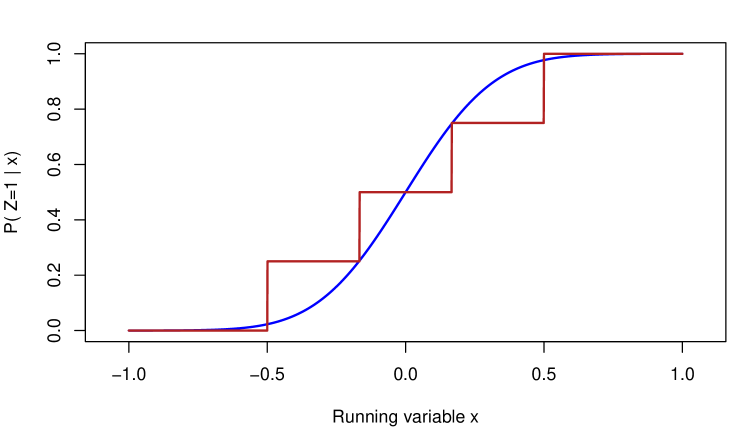
Figure 6: The smooth curve shows a sliding scale with $\Pr(z=1\!\mid\!x)=\Phi(4x)$, where $\Phi$ is the $\mathcal{N}(0,1)$ cumulative distribution function. The step function has $\Pr(z=1\!\mid\!x)$ increasing from $0$ in steps.

Suppose first that $p(x)$ satisfies $p(x)=1-p(-x)$ and is non-decreasing. For instance, $p$ could be the cumulative distribution function (CDF) of a symmetric distribution. A proper CDF would ordinarily have $p(-1)=0$ and $p(1)=1$ too, but we do not need to impose that. With this $p(x)$, the expected number of treated cases is $N/2$. The variance-covariance matrix of $\hat{\beta}$ in our model is then the same as in (3) with $\phi(\Delta)$ replaced by

$$\overline{zx}\equiv\frac{1}{2}\int_{-1}^{1}x\mathbb{E}(z\!\mid\!x)\,\mathrm{d}x=\frac{1}{2}\int_{-1}^{1}x(2p(x)-1)\,\mathrm{d}x.$$

For symmetric $p$, $\overline{z}=(1/2)\int_{-1}^{1}(2p(x)-1)\,\mathrm{d}x=0$ and $\overline{zx^{2}}=(1/2)\int_{-1}^{1}x^{2}(2p(x)-1)\,\mathrm{d}x=0$.

Now let’s consider the expected gain on the $N$ subjects in the trial. The short term gain, averaged over $z$, is

$$\frac{1}{2}\int_{-1}^{1}\beta_{0}+\beta_{1}x+\beta_{2}\mathbb{E}(z\!\mid\!x)\,\mathrm{d}x=\beta_{0}+\beta_{3}\overline{zx}.$$

Supposing as before that $\beta_{3}>0$, we see that the tradeoff between immediate value and information gained is driven by the single variable $\overline{zx}$ and not by whether $\mathbb{E}(z\!\mid\!x)$ is on a continuous sliding scale or simply at three levels $0$, $0.5$ and $1.0$. For tie-breaker designs $\overline{zx}=(1-\Delta^{2})/2\in[0,1/2]$ for $0\leqslant\Delta\leqslant 1$. If $p(x)$ is symmetric then we find that

$$\overline{zx}=2\int_{0}^{1}xp(x)\,\mathrm{d}x-\frac{1}{2}.$$

For $x>0$, we know that $1/2=p(0)\leqslant p(x)\leqslant 1$. It follows that $0\leqslant\overline{zx}\leqslant 1/2$. In other words, the full range of exploration-exploitation tradeoffs available from a sliding scale with symmetric $p(x)$ is already available in a tie-breaker design.

Now suppose that we relax the symmetry constraint on $p(x)$, while still having 50% allocation, that is $\bar{z}=0$. The short term gain still depends only on $\overline{zx}$. The other ingredient in the tradeoff is $\mathrm{Var}(\hat{\beta})$ which depends on $\bar{z}$, $\overline{zx}$ and $\overline{zx^{2}}$. To see what can be gained by symmetrizing we compare $p(x)$ to a symmetric alternative $\tilde{p}(x)=(p(x)+1-p(-x))/2$. This has $\tilde{p}(x)+\tilde{p}(-x)=1$, and so $\tilde{p}$ is symmetric as described above. Denote the result of replacing $p$ by $\tilde{p}$ in the definitions of $\bar{z}$, $\overline{zx}$ and $\overline{zx^{2}}$ by $\tilde{z}$, $\widetilde{zx}$ and $\widetilde{zx^{2}}$, respectively. We find that $\tilde{z}=\bar{z}$ and $\overline{zx}=\widetilde{zx}$, and so symmetrizing has not changed these quantities. However, symmetrizing makes $\widetilde{zx^{2}}=0$ which is not necessarily equal to $\overline{zx^{2}}$. We will see that $\overline{zx^{2}}$ enters our expression for $\mathrm{Var}(\hat{\beta})$ only through $\overline{zx^{2}}^{2}\geqslant\widetilde{zx^{2}}^{2}=0$.

After some algebra our expression for $N\mathrm{Var}(\hat{\beta})$ yields

$$N\mathrm{Var}\begin{pmatrix}\hat{\beta}_{0}\\ \hat{\beta}_{1}\end{pmatrix}\doteq N\mathrm{Var}\begin{pmatrix}\hat{\beta}_{2}\\ \hat{\beta}_{3}\end{pmatrix}\doteq(A-BA^{-1}B)^{-1}$$

where

$$A=\begin{pmatrix}1&0\\ 0&\frac{1}{3}\end{pmatrix}\quad\text{and}\quad B=\begin{pmatrix}\overline{z}^{2}+3\overline{zx}^{2}&\overline{z}\,\overline{zx}+3\overline{zx}\,\overline{zx^{2}}\\ \overline{z}\,\overline{zx}+3\overline{zx}\,\overline{zx^{2}}&\overline{zx}^{2}+3\overline{zx^{2}}^{2}\end{pmatrix}.$$

Then

$$\begin{split}\mathrm{Var}(\hat{\beta}_{1})&\doteq\mathrm{Var}(\hat{\beta}_{3})\doteq\frac{1}{N}\frac{1-3\overline{zx}^{2}}{D},\quad\text{and}\\ \mathrm{Var}(\hat{\beta}_{0})&\doteq\mathrm{Var}(\hat{\beta}_{2})\doteq\frac{1}{N}\frac{1/3-\overline{zx}^{2}-3\overline{zx^{2}}^{2}}{D},\end{split}$$ (15)

for a determinant

$$D=\frac{1}{3}-2\overline{zx}^{2}-3\overline{zx^{2}}^{2}+3\overline{zx}^{4}.$$

Symmetrizing can increase but not decrease $D$ because $\widetilde{zx^{2}}^{2}=0$. Symmetrizing does not change the numerators for $\hat{\beta}_{1}$ and $\hat{\beta}_{3}$ and so it can reduce but not increase their approximate variance expressions. The cases of $\hat{\beta}_{0}$ and $\hat{\beta}_{2}$ are more complicated because symmetrizing changes both their numerators and denominators. However some straightforward calculus shows that those expressions are minimized when $\overline{zx^{2}}^{2}=0$ so they cannot be increased by symmetrization.

It is possible that $\mathrm{Var}(c^{\mathsf{T}}\hat{\beta})$ can be increased by symmetrization for some values of $c\in\mathbb{R}^{4}$. An example of this type can be constructed with $p(x)=|x|$ and $\tilde{p}(x)=1/2$. Then $\mathrm{Var}(\hat{\beta}_{1}+\hat{\beta}_{3})$ is increased under symmetrization. The same holds for $\mathrm{Var}(\hat{\beta}_{2}+\hat{\beta}_{3})$ where $\hat{\beta}_{2}+\hat{\beta}_{3}$ is half of the expected treatment gain at $x=1$.

The most consequential coefficient is $\beta_{3}$. A symmetric sliding scale cannot improve its estimation compared to a tie-breaker design at a given short term cost. A non-symmetric sliding scale cannot improve over a symmetric one when half of the cases are treated. Thus, when half of the cases are to be treated, the original tie-breaker design is optimal at any given level of $\overline{zx}$.

One drawback of using treatment probabilities $0$ and $0.5$ and $1$ is that some of the potential treatment allocations are deterministic. Methods based on the potential outcomes framework (see Imbens and Rubin (2015)) cannot then be readily applied. We could instead use three levels $\epsilon$, $0.5$ and $1-\epsilon$ with the central $\Delta$ of subjects having $p(x)=0.5$. Then we find that the critical quantity governing both statistical and allocation efficiency becomes

$$\overline{zx}=\frac{1}{2}\int_{-1}^{-\Delta}x(2\epsilon-1)\,\mathrm{d}x+\frac{1}{2}\int_{\Delta}^{1}x(2(1-\epsilon)-1)\,\mathrm{d}x=(1-\epsilon)\frac{1-\Delta^{2}}{2}.$$

The consequence is that we can find a design only in the range $0\leqslant\overline{zx}\leqslant(1-\epsilon)/2$ instead of $0\leqslant\overline{zx}\leqslant 1/2$. For small $\epsilon$, this is only a mild reduction in the attainable range, and it still requires only three levels of treatment probability.

8 General numerical approach

The two line model for an assignment variable $x$ with a symmetric distribution made it simple to study central experimental windows of the form $(-\Delta,\Delta)$. In that setting the means of $x_{i}$ and $z_{i}$ were both zero, and the variance of parameter estimates depended simply on just one quantity $\Delta$. We may want to use a more general regression model, allow experimental windows that are not centered around the middle value of $x$, have $x$ values that are not uniform or Gaussian, and we might also want to use models other than two regression lines.

There might even be more than one assignment variable as in Abdulkadiroglu et al. (2017). The price for this flexibility is high; users have to answer some hard questions about their goals, and then do numerical optimization over parameters with a potentially expensive Monte Carlo inner loop. In this section we show that the inner loop can be done algebraically. We also find that the full experiment $\Delta=1$ with $\Pr(z_{i}=1)=1/2$ is variance optimal.

We suppose that prior to treatment assignment, subject $i$ has a known feature vector $F_{i}\in\mathbb{R}^{d}$ which includes an intercept variable equal to $1$, but not the treatment variable $z_{i}$. For instance in the linear and quadratic models, the features $F_{i}$ are $(1,x_{i})^{\mathsf{T}}$ and $(1,x_{i},x_{i}^{2})^{\mathsf{T}}$, respectively. In the regression model

$$Y_{i}=F_{i}^{\mathsf{T}}\beta+z_{i}F_{i}^{\mathsf{T}}\gamma+\varepsilon_{i},$$

we have $\mathbb{E}(Y_{i})=F_{i}^{\mathsf{T}}(\beta+\gamma)$ for the treated subjects $i$ and $\mathbb{E}(Y_{i})=F_{i}^{\mathsf{T}}(\beta-\gamma)$ for the others. Here $\gamma\in\mathbb{R}^{d}$ models the effect of treatment.

The generalized tie-breaker study works with a vector $\theta\in\mathbb{R}^{d}$ and sets

$$\Pr(z_{i}=1\!\mid\!x_{i})=\begin{cases}\phantom{-}1,&\theta^{\mathsf{T}}F_{i}\geqslant\Delta\\ \phantom{-}p,&|\theta^{\mathsf{T}}F_{i}|<\Delta\\ -1,&\theta^{\mathsf{T}}F_{i}\leqslant-\Delta,\end{cases}$$

for some fixed $p\in(0,1)$, not necessarily $1/2$. Because $F_{i}$ contains an intercept term, the experimental window $|\theta^{\mathsf{T}}F_{i}|<\Delta$ need not be centered on a central value of $\theta^{\mathsf{T}}F_{i}$. The analyst must now choose $\Delta\geqslant 0$, $\theta\in\mathbb{R}^{d}$ and $p\in(0,1)$.

The analogue of our previous approach is to find the matrix $(\mathcal{X}^{\mathsf{T}}\mathcal{X})^{-1}$ where

$$\mathcal{X}^{\mathsf{T}}\mathcal{X}=\begin{pmatrix}A&B\\ B&A\end{pmatrix},\quad A=\sum_{i}F_{i}F_{i}^{\mathsf{T}},\quad B=\sum_{i}w_{i}F_{i}F_{i}^{\mathsf{T}},$$

for

$$w_{i}=\mathbb{E}(z_{i}\!\mid\!F_{i})=\begin{cases}1,&\theta^{\mathsf{T}}F_{i}\geqslant\Delta,\\ 2p-1,&|\theta^{\mathsf{T}}F_{i}|<\Delta,\\ -1,&\theta^{\mathsf{T}}F_{i}\leqslant-\Delta.\end{cases}$$

The lower right corner of $\mathcal{X}^{\mathsf{T}}\mathcal{X}$ is $A$ because $\mathbb{E}(z_{i}^{2}\!\mid\!F_{i})=1$. Averaging over the outcomes of $z_{i}$ this way is statistically reasonable when $N\gg d$. If $\varepsilon_{i}$ are independent with mean zero and variance $\sigma^{2}$, then

$$\mathrm{Var}\left(\begin{pmatrix}\hat{\beta}\\ \hat{\gamma}\end{pmatrix}\right)=(\mathcal{X}^{\mathsf{T}}\mathcal{X})^{-1}\sigma^{2}.$$

This averages over the outcomes $\varepsilon_{i}$ so that they do not have to be simulated.

One can now do brute force numerical search for good values of $\theta$ and $p$ and $\Delta$. A good choice would yield a favorably small $\mathrm{Var}(\hat{\gamma})$. A bad choice will yield a larger variance covariance matrix. A very bad choice would lead to singular $\mathcal{X}^{\mathsf{T}}\mathcal{X}$ and one would of course reject the corresponding triple $(\theta,\Delta,p)$. For instance, such a singularity would happen if $\max_{i}\theta^{\mathsf{T}}F_{i}<-\Delta$ which is an obviously poor choice because then no subjects would be in the treatment group.

Using a formula for the inverse of a block matrix we get

$$\mathrm{Var}(\hat{\gamma})=\mathrm{Var}(\hat{\beta})=(A-BA^{-1}B)^{-1}\sigma^{2}$$

and $\mathrm{Cov}(\hat{\beta},\hat{\gamma})=-A^{-1}B(A-BA^{-1}B)^{-1}\sigma^{2}$. In an RCT with $p=1/2$ we have $B=0$. For $\Delta<\max_{i}(|\theta^{\mathsf{T}}F_{i}|)$ certain components of $B$ become nonzero. That can increase $BA^{-1}B$ but not decrease it. As a consequence, $\mathrm{Var}(\hat{\gamma})$ cannot be made smaller than it is under the RCT for any choice of $\Delta$ given $\theta$, when $p=1/2$.

9 Non-central experimental regions

Our treatment of the two line model assumed that the experimental region was in the center of the range of the assignment variable. A customer loyalty program might well reward just the top few customers and a scholarship program will ordinarily award scholarships to fewer than half of the students. We analyze that case and compare statistical efficiency of a tie-breaker design in the upper quantiles to an RDD there. We find that the tie-breaker experimenting on the second decile is about $1.62$ times as efficient as an RDD with a threshold at the 85’th percentile, both of which offer the treatment to 15% of subjects. If we find upon seeing the data that the linear model is too biased and reduce the bias by only looking at the top $30$% of data, then on that data subset, using the tie-breaker becomes $1.63$% times as efficient as the RDD. That is, the efficiency is virtually the same.

To handle designs where fewer than half of the subjects are treated we let

$$\Pr(z_{i}=1\!\mid\!x_{i})=\begin{cases}\phantom{-}1,&x_{i}\geqslant b\\ \phantom{-}p,&a<x_{i}<b\\ -1,&x_{i}\leqslant a\end{cases}$$ (16)

for $a\leqslant b$ and $0<p<1$. We abuse notation a little by having the function $p(x)$ subsume all three cases in (16). For a less expensive treatment we might want to offer it to the top $50$% of subjects and then randomize it to the bottom $50$% and (16) can handle this choice too.

Let the assignment variable $x\in\mathbb{R}$ be random with $\mathbb{E}(x^{4})<\infty$. Then letting $\mathcal{X}$ be the design matrix in the two line regression, and noting that $z^{2}=1$, we have

$$\frac{1}{N}\mathcal{X}^{\mathsf{T}}\mathcal{X}=\begin{pmatrix}1&\mathbb{E}(x)&\mathbb{E}(z)&\mathbb{E}(xz)\\ \mathbb{E}(x)&\mathbb{E}(x^{2})&\mathbb{E}(xz)&\mathbb{E}(x^{2}z)\\ \mathbb{E}(z)&\mathbb{E}(xz)&1&\mathbb{E}(x)\\ \mathbb{E}(xz)&\mathbb{E}(x^{2}z)&\mathbb{E}(x)&\mathbb{E}(x^{2})\\ \end{pmatrix}+O_{p}\Bigl{(}\frac{1}{\sqrt{N}}\Bigr{)}$$

under random sampling of $x_{i}$ and $z_{i}$ given $x_{i}$ for $i=1,\dots,N$. The $O_{p}(N^{-1/2})$ error holds because $\mathbb{E}(x^{4})<\infty$. The error could be $o_{p}(N^{-1/2})$ if $p(x)$ is a simple enough function to make stratification tractable.

We can center $x$ so that $\mathbb{E}(x)=0$ and then

$$\mathrm{Var}(\hat{\beta})\doteq\frac{1}{N}\begin{pmatrix}D&C\\ C&D\end{pmatrix}^{-1},\ \text{for}\ \,C=\begin{pmatrix}\mathbb{E}(z)&\mathbb{E}(xz)\\ \mathbb{E}(xz)&\mathbb{E}(x^{2}z)\\ \end{pmatrix}\ \,\text{and}\ \,D=\begin{pmatrix}1&0\\ 0&\mathbb{E}(x^{2})\\ \end{pmatrix}.$$

We can scale $x$ to get $\mathbb{E}(x^{2})=1$ so that $D=I_{2}$. We retain more general scaling because $x\sim\mathcal{U}[-1,1]$ has $\mathbb{E}(x^{2})=1/3$ and rescaling would require working with the less convenient distribution $\mathcal{U}[-\sqrt{3},\sqrt{3}]$.

We need the inverse of a block diagonal matrix containing just two unique square blocks. The following proposition specializes block matrix inversion to our case.

Proposition 3.

Let $D$ be an invertible matrix and $C$ be a square matrix with the same dimensions as $D$. If $D-CD^{-1}C$ is invertible, then

$$\begin{pmatrix}D&C\\ C&D\end{pmatrix}^{-1}=\begin{pmatrix}A&B\\ B&A\end{pmatrix}$$

for $A=(D-CD^{-1}C)^{-1}$ and $B=-ACD^{-1}$.

Proof.

Multiplying,

$$\begin{pmatrix}A&B\\ B&A\end{pmatrix}\begin{pmatrix}D&C\\ C&D\end{pmatrix}=\begin{pmatrix}AD+BC&AC+BD\\ BD+AC&BC+AD\end{pmatrix}.$$

Now $AC+BD=AC-ACD^{-1}D=0$ and $AD+BC=A(D-CD^{-1}C)=I$. ∎

Using Proposition 3 we get

$$\mathrm{Var}(\hat{\beta})\doteq\frac{1}{N}\begin{pmatrix}\phantom{-}(D-CD^{-1}C)^{-1}\phantom{CD^{-1}}&-(D-CD^{-1}C)^{-1}CD^{-1}\\ -(D-CD^{-1}C)^{-1}CD^{-1}&\phantom{-}(D-CD^{-1}C)^{-1}\phantom{CD^{-1}}\\ \end{pmatrix}.$$

Our primary interest is in $\mathrm{Var}(\hat{\beta}_{3})$, for the coefficient of $xz$. This is the lower right element of $(D-CD^{-1}C)^{-1}$. Now

$$D-CD^{-1}C =\begin{pmatrix}1-\mathbb{E}(z)^{2}-\mathbb{E}(xz)^{2}/\mathbb{E}(x^{2})&-\mathbb{E}(xz)\mathbb{E}(z)-\mathbb{E}(x^{2}z)\mathbb{E}(xz)/\mathbb{E}(x^{2})\\ -\mathbb{E}(xz)\mathbb{E}(z)-\mathbb{E}(x^{2}z)\mathbb{E}(xz)/\mathbb{E}(x^{2})&\mathbb{E}(x^{2})-\mathbb{E}(xz)^{2}-\mathbb{E}(x^{2}z)^{2}/\mathbb{E}(x^{2})\\ \end{pmatrix}$$

$$\equiv\begin{pmatrix}M_{11}&M_{12}\\ M_{12}&M_{22}\end{pmatrix},$$

and so

$$\mathrm{Var}(\hat{\beta}_{3})=\frac{1}{N}\frac{M_{11}}{M_{11}M_{22}-M_{12}^{2}}.$$

The asymptotic value of $N\mathrm{Var}(\hat{\beta}_{3})$ depends on certain integrals. For the case of primary interest to us with $x\sim\mathcal{U}[-1,1]$, and $p(x)=1/2$ in the experimental region, these are

$$\mathbb{E}(x^{2}) =\frac{1}{2}\int_{-1}^{1}x^{2}\,\mathrm{d}x=\frac{1}{3},$$

$$\mathbb{E}(xz) =\frac{1}{2}\int_{-1}^{a}(-x)\,\mathrm{d}x+\frac{1}{2}\int_{b}^{1}x\,\mathrm{d}x=\frac{1}{2}-\frac{a^{2}+b^{2}}{4},$$

$$\mathbb{E}(z) =-\frac{1}{2}(a+1)+\frac{1}{2}(1-b)=-\frac{a+b}{2},\quad\text{and}$$

$$\mathbb{E}(x^{2}z) =\frac{1}{2}\int_{-1}^{a}(-x^{2})\,\mathrm{d}x+\frac{1}{2}\int_{b}^{1}x^{2}\,\mathrm{d}x=-\frac{a^{3}+b^{3}}{6}.$$

Method	$a\ \,$	$b\ \,$	$\mathrm{Var}(\hat{\beta}_{3})$
Experiment	$-1.00$	$1.00$	$3.00/N$
RDD	$0.00$	$0.00$	$12.00/N$
Bottom 50%	$-1.00$	$0.00$	$13.09/N$
Skew RDD (85th)	$0.70$	$0.70$	$223.44/N$
Second 10%	$0.60$	$0.80$	$137.56/N$

Table 2: Variance of $\hat{\beta}_{3}$ (treatment effect slope) for some central and non-central experimental regions.

Table 2 shows $\mathrm{Var}(\hat{\beta}_{3})$ for various designs when $x\sim\mathcal{U}[-1,1]$. The first two are the full experiment and the RDD discussed previously. Next is an experiment on just the bottom half of $x$. This strategy is inadmissible by our criteria. It has more variance than the RDD and also lower allocation efficiency.

Next, the table compares some options we might have when only $15$% of subjects can get the treatment. The first one is to do an RDD with the critical point at the $85$’th percentile. Alternatively we could choose a tie-breaker design giving the top $10$% of subjects the treatment along with a randomly chosen half of the second $10$% of customers. The skewed RDD has $223.44/137.56\doteq 1.62$ times the variance for $\hat{\beta}_{3}$ compared to running the tie-breaker on the second $10$%. Put another way, the tie-breaker design reduces $\mathrm{Var}(\hat{\beta}_{3})$ by a factor of roughly $0.6$.

In a setting like this we might find after gathering the data that the working linear model fits poorly over the whole range of $x$ and the model would then have severe bias. An alternative is to just analyze the top $30$% of subjects. In that case, the skewed RDD becomes a usual RDD and the tie-breaker becomes an experiment with $\Delta=1/3$. Working on only $30$% as many observations over a narrower range of $x$ values will increase the variance for both models. The efficiency of this tie-breaker compared to the RDD is $1+3(1/3)^{2}(2-(1/3)^{2})\doteq 1.63$, almost identical to what we find for the designs in the table.

10 Discussion

In an incentive plan, a regression discontinuity design rewards the a priori best customers but it has severe disadvantages if one wants to follow up with regression models to measure impact. There is a tradeoff between estimation efficiency and allocation efficiency. Proposition 1 provides a principled way to translate estimates or educated guesses about the present value of the incentives and future value of information into a choice of $\Delta$ in a hybrid experiment.

In commercial settings, the incentive under study will change over time. Experience with similar though perhaps not identical prior incentive plans then gives some guidance for making the tradeoff. A simpler approach is to do the smallest experiment with at least some given fraction of the information from $\Delta=1$.

We have examined a simple linear model because it is easiest to work with and is a reasonable design choice in many contexts. Analysts have many more models at their disposal when the data come in and they do not need to use that model. If a more satisfactory model is found then the methods of Section 8 can be used to design the next experiment under that model. Section 5 on the quadratic model provides a warning: the RDD becomes very unreliable already with this model which is only slightly more complicated than the two-line model. A tie-breaker greatly reduces the variance compared to RDD.

In some applications, the assignment variable may be the output of a scoring model based on many subject variables. We expect that incorporating randomness into the design will give better data for refitting such an underlying scoring model, but following up that point is outside the scope of this article. The effects are likely to vary considerably from problem to problem.

References

- Abdulkadiroglu et al. (2017) Atila Abdulkadiroglu, Joshua D Angrist, Yusuke Narita, and Parag A Pathak. Impact evaluation in matching markets with general tie-breaking. Technical report, National Bureau of Economic Research, 2017. URL http://www.nber.org/papers/w24172.
- Aiken et al. (1998) Leona S Aiken, Stephen G West, David E Schwalm, James L Carroll, and Shenghwa Hsiung. Comparison of a randomized and two quasi-experimental designs in a single outcome evaluation: Efficacy of a university-level remedial writing program. Evaluation Review, 22(2):207–244, 1998.
- Angrist et al. (2014) Joshua Angrist, Sally Hudson, and Amanda Pallais. Leveling up: Early results from a randomized evaluation of post-secondary aid. Technical report, National Bureau of Economic Research, 2014. URL http://www.nber.org/papers/w20800.pdf.
- Angrist and Pischke (2009) Joshua D. Angrist and Jorn-Steffen Pischke. Mostly Harmless Econometrics. Princeton Univerity Press, Princeton, 2009.
- Angrist and Pischke (2014) Joshua D. Angrist and Jorn-Steffen Pischke. Mastering Metrics. Princeton Univerity Press, Princeton, 2014.
- Armstrong and Kolesár (2018) Timothy B Armstrong and Michal Kolesár. Optimal inference in a class of regression models. Econometrica, 86(2):655–683, 2018.
- Box et al. (1978) George E. P. Box, William Gordon Hunter, and J. Stuart Hunter. Statistics for experimenters. John Wiley and Sons, New York, 1978.
- Calonico et al. (2014) Sebastian Calonico, Matias D Cattaneo, and Rocio Titiunik. Robust nonparametric confidence intervals for regression-discontinuity designs. Econometrica, 82(6):2295–2326, 2014.
- Campbell (1969) Donald T Campbell. Reforms as experiments. American psychologist, 24(4):409, 1969.
- Cappelleri and Trochim (2003) Joseph C. Cappelleri and William M. K. Trochim. Cutoff designs. In Marcel Dekker, editor, Encyclopedia of Biopharmaceutical Statistics. CRC Press, 2003. doi: 10.1081/E-EBS12000734. URL https://www.socialresearchmethods.net/research/Cutoff%20Designs%202003.pdf.
- Gelman and Imbens (2017) Andrew Gelman and Guido Imbens. Why high-order polynomials should not be used in regression discontinuity designs. Journal of Business & Economic Statistics, 0(0), 2017. URL http://www.nber.org/papers/w20405.
- Goldberger (1972) A. S. Goldberger. Selection bias in evaluating treatment effects: Some formal illustrations. Technical Report Discussion paper 128–72, Institute for Research on Poverty, University of Wisconsin–Madison, 1972.
- Hahn et al. (2001) Jinyong Hahn, Petra Todd, and Wilbert Van der Klaauw. Identification and estimation of treatment effects with a regression-discontinuity design. Econometrica, 69(1):201–209, 2001.
- Imbens and Lemieux (2008) Guido Imbens and Thomas Lemieux. Regression discontinuity designs: a guide to practice. Journal of Econometrics, 142(2):615–635, 2008. URL www.nber.org/papers/w13039.pdf.
- Imbens and Wager (2019) Guido Imbens and Stefan Wager. Optimized regression discontinuity designs. Review of Economics and Statistics, 101(2):264–278, 2019.
- Imbens and Rubin (2015) Guido W Imbens and Donald B Rubin. Causal inference in statistics, social, and biomedical sciences. Cambridge University Press, 2015.
- Jacob et al. (2012) Robin Tepper Jacob, Pei Zhu, Marie-Andrée, Somers, and Howard Bloom. A practical guide to regression discontinuity. MDRC Publications, July 2012. URL https://www.mdrc.org/publication/practical-guide-regression-discontinuity.
- Lee and Lemieux (2010) David S. Lee and Thomas Lemieux. Regression discontinuity designs in economics. Journal of Economic Literature, 48:281–355, June 2010. URL https://www.princeton.edu/~davidlee/wp/RDDEconomics.pdf.
- McCrary (2008) Justin McCrary. Manipulation of the running variable in the regression discontinuity design: A density test. Journal of econometrics, 142(2):698–714, 2008.
- Porter (2003) Jack Porter. Estimation in the regression discontinuity model. Unpublished Manuscript, Department of Economics, University of Wisconsin at Madison, 2003:5–19, 2003.
- Rice and Rosenblatt (1983) John Rice and Murray Rosenblatt. Smoothing splines: regression, derivatives and deconvolution. The annals of Statistics, pages 141–156, 1983.
- Rosenman and Rajkumar (2019) Evan Rosenman and Karthik Rajkumar. Optimized partial identification bounds for regression discontinuity designs with manipulation. Technical Report arXiv:1910.02170, Stanford University, 2019.
- Scott (2015) Steven L. Scott. Multi-armed bandit experiments in the online service economy. Applied Stochastic Models in Business and Industry, 31(1):37–45, 2015.
- Student (1931) Student. The Lanarkshire milk experiment. Biometrika, 23(2/3):398–406, 1931.
- Thistlethwaite and Campbell (1960) D. L. Thistlethwaite and D. T. Campbell. Regression-discontinuity analysis: An alternative to the ex post facto experiment. Journal of Educational psychology, 51(6):309, 1960.
- Van Der Klaauw (2008) Wilbert Van Der Klaauw. Regression–discontinuity analysis: A survey of recent developments in economics. LABOUR, 22(2):219–245, 2008. URL http://citeseerx.ist.psu.edu/viewdoc/download?doi=10.1.1.466.956&rep=rep1&type=pdf.
- Wu and Hamada (2011) C. F. Jeff Wu and Michael S. Hamada. Experiments: planning, analysis, and optimization. John Wiley & Sons, New York, 2011.