Generalization of Bloch’s theorem for arbitrary boundary conditions:
Interfaces and topological surface band structure

Abstract

We describe a method for exactly diagonalizing clean $D$-dimensional lattice systems of independent fermions subject to arbitrary boundary conditions in one direction, as well as systems composed of two bulks meeting at a planar interface. The specification of boundary conditions and interfaces can be easily adjusted to describe relaxation, reconstruction, or disorder away from the clean bulk regions of the system. Our diagonalization method builds on the generalized Bloch theorem [A. Alase et al., Phys. Rev. B 96, 195133 (2017)] and the fact that the bulk-boundary separation of the Schrödinger equation is compatible with a partial Fourier transform operation. Bulk equations may display unusual features because they are relative eigenvalue problems for non-Hermitian, bulk-projected Hamiltonians. Nonetheless, they admit a rich symmetry analysis that can simplify considerably the structure of energy eigenstates, often allowing a solution in fully analytical form. We illustrate our extension of the generalized Bloch theorem to multicomponent systems by determining the exact Andreev bound states for a simple SNS junction. We then analyze the Creutz ladder model, by way of a conceptual bridge from one to higher dimensions. Upon introducing a new Gaussian duality transformation that maps the Creutz ladder to a system of two Majorana chains, we show how the model provides a first example of a short-range chiral topological insulators hosting topological zero modes with a power-law profile. Additional applications include the complete analytical diagonalization of graphene ribbons with both zigzag-bearded and armchair boundary conditions, and the analytical determination of the edge modes in a chiral $p+ip$ two-dimensional topological superconductor. Lastly, we revisit the phenomenon of Majorana flat bands and anomalous bulk-boundary correspondence in a two-band gapless $s$-wave topological superconductor. Beside obtaining sharp indicators for the presence of Majorana modes through the use of the boundary matrix, we analyze the equilibrium Josephson response of the system, showing how the presence of Majorana flat bands implies a substantial enhancement in the $4\pi$-periodic supercurrent.

I Introduction

This paper is the logical continuation of Ref. [PRB1, ], referred to as Part I henceforth. In Part I, we described a method for the exact diagonalization of clean systems of independent fermions subject to arbitrary boundary conditions (BCs), and illustrated its application in several prototypical one-dimensional ($D=1$) tight-binding models PRB1 ; JPA ; PRL . Our broad motivation was, and remains, to develop an analytic approach for exploring and quantitatively characterizing the interplay between bulk and boundary physics, in a minimal setting where translation symmetry is broken only by BCs. On a fundamental level, such an understanding is a prerequisite toward building a complete physical picture of the bulk-boundary correspondence for mean-field topological electronic matter. For systems classified as topologically non-trivial chiu16 , there exist at least one bulk invariant and one boundary invariant whose values must coincide prodanBook . Bulk invariants are insensitive to BCs by construction, but what is the impact of BCs on boundary invariants? Likewise, with an eye toward applications, what are design principles and ultimate limitations in engineering boundary modes in topological materials?

Our method of exact diagonalization provides an insightful first step towards answering these questions, because it can be casted neatly as a generalization of Bloch’s theorem to arbitrary BCs. As we showed, in the generic case the exact energy eigenstates of a single-particle Hamiltonian are linear combinations of generalized Bloch states. The latter are uniquely determined by the analytic continuation of the Bloch Hamiltonian (or some closely-related matrix function) off the Brillouin zone to complex values of the crystal momentum. In essence, the problem of diagonalizing the single-particle Hamiltonian boils down to finding all linear combinations of generalized Bloch states which satisfy the BCs. As long as the bulk is disorder-free and couplings have finite range, BCs can be encoded in a boundary matrix, whose shape is generally independent of the number of lattice sites. Any change in the energy levels and eigenstates induced by a change in BCs is thus directly and efficiently computable from the boundary matrix in principle.

The generalized Bloch theorem properly accounts for two types of energy eigenstates that do not exist once translation invariance is imposed via Born-von-Karman (periodic) BCs: perfectly localized modes and localized modes whose exponential decay exhibits a power-law prefactor. While such “power-law modes” have been well documented in numerical investigations of long-ranged tight-binding models longrange , it was a surprise to find them in short-range modelsPRB1 ; JPA – notably, the topological zero-modes of the Majorana chain display power-law behavior in a parameter regime known as the “circle of oscillations”. As shown in Part I, both types of exotic modes appear precisely when the transfer matrix of the model fails to be invertible. The generalized Bloch theorem may be thought of as bestowing exact solvability in the same sense as the algebraic Bethe ansatz does: the linear-algebraic task of diagonalizing the single-particle Hamiltonian is mapped to one of solving a small (independent of the number of sites) system of polynomial equations. While in general, if the polynomial degree is higher than four, the roots must be found numerically, whenever this polynomial system can be solved analytically, one has managed to solve the original linear-algebraic problem analytically as well. In fact, fully analytical solutions are less rare than one might think, and either emerge in special parameter regimes, or by suitably adjusting BCs.

In this paper, Part II, we extend the scope of our generalized Bloch theorem even further, with a twofold goal in mind. First, while in Part I we presented the basic framework for calculating energy eigenstates of fermionic $D$-dimensional lattice systems with surfaces, for simplicity we restricted to a setting where the total system Hamiltonian retains translation invariance along $D-1$ directions parallel to the surfaces. In more realistic situations in surface physics, however, this assumption is invalidated by various factors, including surface reconstruction and surface disorder. Establishing procedures for exact diagonalization of $D$-dimensional clean systems subject to arbitrary BCs (surface disorder included) on two parallel hyperplanes is thus an important necessary step. We accomplish this in Sec. II, by allowing for BCs to be adjusted in order to conveniently describe surface relaxation, reconstruction, or disorder in terms of an appropriate boundary matrix.

As a second main theoretical extension, we proceed to show in Sec. III how to diagonalize “multi-component” systems that host hyperplanar interfaces separating clean bulks, that is, “junctions”. Surface and interface problems are conceptually related: BCs are but effective models of the interface between the system of interest and its “complement” or environment. While it is well appreciated that exotic many-body phenomena can take place at interfaces, there are essentially no known principles to guide interface engineering (see e.g. Ref. [diez15, ] for an instructive case study). It is our hope that our characterization of interfaces in terms of interface matrices will shed some light on the problem of finding such guiding principles, at least within the mean-field approximation. As a concrete illustration, we include an exact calculation of the Andreev bound states in a simple model of a clean superconducting-normal-superconducting (SNS) junction, complementing the detailed numerical investigations reported in Ref. [bena12, ].

In addition to the SNS junction, we provide in Sec. IV several explicit applications of our diagonalization procedures to computing surface band structures in systems ranging from insulating ladders to $p$- and and $s$-wave topological superconductors (TSCs) in $D=2$ lattices. The ladder model of domain-wall fermions introduced by Creutz Creutz ; CreutzPRD ; CreutzRMP serves as a bridge between one to higher dimensions. For some values of the magnetic flux, the Creutz ladder can be classified as a topological insulator in class A and we find that it displays topological power-law modes. To the best of our knowledge, this is the first example of such power-law modes in a short-range insulator. In addition, we uncover a Gaussian duality mapping the Creutz ladder to a dual system consisting of two Majorana chains (see Ref. [equivalence, ] for other examples of dualities bridging distinct classes in the mean-field topological classification of electronic matter, and Ref. [dualitygeneral, ] for the general approach to dualities).

Moving to $D=2$ systems, we first consider graphene ribbons with two types of edges, “zigzag-bearded” and “armchair” (in the terminology of Ref. [kohmoto07, ]), in order to also provide an opportunity for direct comparison within our method and other analytical calculations in the literature. As a more advanced application, we compute in closed form the surface band structure of the chiral $p+ip$ TSC read00 . This problem is well under control within the continuum approximationbernevig , but not on the lattice. This distinction is important because the phase diagram of lattice models is richer than one would infer from the continuum approximation. As a final, technically harder example of a surface band-structure calculation, we investigate a two-band, gapless $s$-wave TSC that can host symmetry-protected Majorana flat bands and is distinguished by a non-unique, anomalous bulk-boundary correspondence swavePRL ; swavePRB .

We conclude in Sec. V by iterating our key points and highlighting some key open questions. To ease the presentation, most technical details of our calculations are deferred to appendixes, including the analytic diagonalization of several paradigmatic $D=1$ models with boundaries. For reference, a summary of all the model systems we explicitly analyzed so far using the generalized Bloch theorem approach is presented in Table 1.

$D=1$ and quasi-($D$=1) systems	PC	Boundary Conditions	Some Key Results	See
Single-band chain	yes	open/edge impurities	full diagonalization	Part I, Sec. V.A
Anderson model	yes	open	full diagonalization	Part I, Sec. V.B
Majorana Kitaev chain	no	open	full diagonalization	Refs. [PRL, ; JPA, ];
			power-law Majorana modes	Part I, Sec. V.C
Two-band $s$-wave TSC	no	open/twisted	$4\pi$-periodic supercurrent	Part I, Sec VI.B
			without parity switch
BCS chain	no	open	full diagonalization	App. B
Su-Schrieffer-Heeger model	yes	reconstructed	full diagonalization	App. E
Rice-Mele model	yes	reconstructed	full diagonalization	App. E
Aubry-André-Harper model	yes	reconstructed	full diagonalization	App. E
(period-two)
Creutz ladder	yes	open	power-law topological modes	Sec. IV.1, App. D
Majorana ladder	no	open	SC dual of Creutz ladder	Sec. IV.1.1
SNS junction	no	junction	Andreev bound states	Sec. III
$D=2$ systems
Graphene (including	yes	zigzag-bearded (ribbon)	full diagonalization	Sec. IV.2.1
modulated on-site potential)		armchair (ribbon)	full diagonalization	Sec. IV.2.2
Harper-Hofstadter model	yes	open (ribbon)	closed-form edge bands and states	Ref. [Qiaoru, ]
Chiral p+ip TSC	no	open (ribbon)	closed-form edge bands and states	Sec. IV.3
			power-law surface modes
Two-band $s$-wave TSC	no	open/twisted	$k_{\parallel}$-resolved DOS	Sec. IV.4
			localization length at zero energy
			enhanced $4\pi$-periodic supercurrent

Table 1: Summary of representative models analyzed in this work along with Part I (Ref. [PRB1, ]) and Ref. [Qiaoru, ], by using the generalized Bloch theorem approach. Some emerging key results are highlighted in the fourth column. PC: particle-conserving, DOS: density of states, SC: superconductor (or superconducting, depending on context). Additional models that are amenable to solution by our approach include Majorana chains with twisted BCs Katsura17 or longer-range (e.g., next-nearest-neighbor) couplings Liu , dimerized Kitaev chains Zhou , period-three hopping models Kevin , as well as time-reversal-invariant TSC wires with spin-orbit coupling Aligia , to name a few.

II Tailoring the generalized Bloch theorem to surface physics problems

As mentioned, the main aim of this section is to describe how the generalized Bloch theorem may be tailored to encompass BCs encountered in realistic surface-physics scenarios, which need not respect translation invariance along directions parallel to the interface, as we assumed in Part I. Notwithstanding, the key point to note is that the bulk-boundary separation introduced in Part I goes through regardless of the nature of the BCs. As a result, the bulk equation describing a clean system can always be decoupled by a partial Fourier transform into a family of “virtual” chains parametrized by the conserved component of crystal momentum ${\mathbf{k}}_{\parallel}$. If the BCs conserve ${\mathbf{k}}_{\parallel}$, then they also reduce to BCs for each virtual chain. If they do not, then the BCs hybridize the generalized Bloch states associated to the individual virtual chains. In general, the boundary matrix will then depend on all crystal momenta in the surface Brillouin zone.

II.1 Open boundary conditions

We consider a clean system of independent fermions embedded on a $D$-dimensional lattice with associated Bravais lattice $\Lambda_{D}$. Let $d_{\rm int}$ denote the number of fermionic degrees (e.g., the relevant orbital and spin degrees) enclosed by a primitive cell attached to each point of $\Lambda_{D}$. Now let us terminate this system along two parallel lattice hyperplanes, or hypersurfaces henceforth – resulting in open (or “hard-wall”) BCs.

The terminated system is translation-invariant along $D-1$ lattice vectors parallel to the hypersurfaces, so that we can associate with it a Bravais lattice $\Lambda_{D-1}$ of spatial dimension $D-1$, known as the surface mesh bechstedt . If ${\mathbf{m}}_{1},\dots,{\mathbf{m}}_{D-1}$ denote the primitive vectors of $\Lambda_{D-1}$, then any point ${\mathbf{j}}_{\parallel}\in\Lambda_{D-1}$ can be expressed as ${\mathbf{j}}_{\parallel}=\sum_{\mu=1}^{D-1}j_{\mu}{\mathbf{m}}_{\mu}$, where $j_{\mu}$ are integers. Let us choose a lattice vector ${\mathbf{s}}$ of $\Lambda_{D}$ that is not in the surface mesh (and therefore, not parallel to the two hypersurfaces). We will call ${\mathbf{s}}$ the stacking vector. Since $\{{\mathbf{m}}_{1},\dots,{\mathbf{m}}_{D-1},{\mathbf{s}}\}$ are not the primitive vectors of $\Lambda_{D}$ in general, the Bravais lattice $\bar{\Lambda}_{D}$ generated by them may cover only a subset of points in $\Lambda_{D}$. Therefore, in general, each primitive cell of $\bar{\Lambda}_{D}$ may enclose a number $I>1$ of points of $\Lambda_{D}$. As a result, there are a total of $\bar{d}_{\rm int}=Id_{\rm int}$ fermionic degrees of freedom attached to each point ${\mathbf{j}}_{\parallel}+j{\mathbf{s}}$ of $\bar{\Lambda}_{D}$ with $j$ an integer (see Fig. 1). Let us denote the corresponding creation (annihilation) operators by $c^{\dagger}_{{\mathbf{j}}_{\parallel}j1},\dots,c^{\dagger}_{{\mathbf{j}}_{\parallel}j\bar{d}_{\rm int}}$ ($c_{{\mathbf{j}}_{\parallel}j1},\dots,c_{{\mathbf{j}}_{\parallel}j\bar{d}_{\rm int}}$). For each ${\mathbf{j}}_{\parallel}$ in the surface mesh, we define the array of the basis of fermionic operators by

$$\hat{\Phi}^{\dagger}_{{\mathbf{j}}_{\parallel}}\equiv\begin{bmatrix}\hat{\Phi}^{\dagger}_{{\mathbf{j}}_{\parallel},1}&\cdots&\hat{\Phi}^{\dagger}_{{\mathbf{j}}_{\parallel},N}\end{bmatrix},\;\;\hat{\Phi}^{\dagger}_{{\mathbf{j}}_{\parallel},j}\equiv\begin{bmatrix}c^{\dagger}_{{\mathbf{j}}_{\parallel}j1}&\cdots&c^{\dagger}_{{\mathbf{j}}_{\parallel}j\bar{d}_{\rm int}}\end{bmatrix},$$

where the integer $N$ is proportional to the separation between the two hypersurfaces. For arrays, such as $\hat{\Phi}^{\dagger}_{{\mathbf{j}}_{\parallel}}$ and $\hat{\Phi}_{{\mathbf{j}}_{\parallel}}^{\;}$, we shall follow the convention that the arrays appearing on the left (right) of a matrix are row (column) arrays. In the above basis, the many-body Hamiltonian of the system, subject to open BCs on the hypersurfaces, can be expressed as PRB1

$$\widehat{H}_{N}=\sum_{{\mathbf{j}}_{\parallel},{\mathbf{r}}_{\parallel}\in\Lambda_{D-1}}\Big{[}\hat{\Phi}^{\dagger}_{{\mathbf{j}}_{\parallel}}K_{{\mathbf{r}}_{\parallel}}\hat{\Phi}^{\;}_{{\mathbf{j}}_{\parallel}+{\mathbf{r}}_{\parallel}}+\frac{1}{2}(\hat{\Phi}^{\dagger}_{{\mathbf{j}}_{\parallel}}\Delta_{{\mathbf{r}}_{\parallel}}\hat{\Phi}_{{\mathbf{j}}_{\parallel}+{\mathbf{r}}_{\parallel}}^{\dagger}+\text{H.c.})\Big{]},$$

where ${\mathbf{j}}_{\parallel},{\mathbf{r}}_{\parallel}$ are vectors in the surface mesh, and $K_{{\mathbf{r}}_{\parallel}}$, $\Delta_{{\mathbf{r}}_{\parallel}}$ are $N\bar{d}_{\rm int}\times N\bar{d}_{\rm int}$ hopping and pairing matrices that satisfy $K_{-{\mathbf{r}}_{\parallel}}=K_{{\mathbf{r}}_{\parallel}}^{\dagger}$, $\Delta_{-{\mathbf{r}}_{\parallel}}=-\Delta_{{\mathbf{r}}_{\parallel}}^{\rm T}$ by virtue of fermionic statistics, with the superscript ${\rm T}$ denoting the transpose operation. Thanks to the assumptions of clean, finite-range system, these are banded block-Toeplitz matrices JPA : explicitly, if $R\geq 1$ is the range of hopping and pairing, we may write $[S_{{\mathbf{r}}_{\parallel}}]_{jj^{\prime}}\equiv S_{{\mathbf{r}}_{\parallel},j^{\prime}-j}\equiv S_{{\mathbf{r}}_{\parallel},r}$, with

$$S_{{\mathbf{r}}_{\parallel},r}=0\quad\text{if}\quad|r|>R,\;\;\forall{\mathbf{r}}_{\parallel},\quad\mbox{where }S=K,\Delta.$$

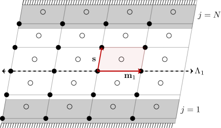
Figure 1: (Color online) Sketch of a $D=2$ lattice system with nearest-neighbor (NN) hopping subject to arbitrary BCs. The filled and hollow circles together form a Bravais lattice $\Lambda_{2}$. The two $D=1$ edges of the system are shown by horizontal lines decorated by pattern. The surface mesh $\Lambda_{1}$ is generated by ${\mathbf{m}}_{1}$, and consists of all points connected by dashed black lines. ${\mathbf{m}}_{1}$ and ${\mathbf{s}}$ generate the Bravais lattice $\bar{\Lambda}_{2}$, formed only by the filled circles. A primitive cell of $\bar{\Lambda}_{2}$ (shaded brown) encloses two points of $\Lambda_{2}$. In this case, assuming there are $d_{\rm int}$ internal degrees associated to each point of $\Lambda_{2}$, we get $\bar{d}_{\rm int}=2d_{\rm int}$. Since, for NN hopping, $R=1$, the operator $W$ that implements the BCs has its support on single-particle states in the boundary region (shaded gray).

Next, we enforce periodic BCs along the directions ${\mathbf{m}}_{1},\dots,{\mathbf{m}}_{D-1}$ in which translation invariance is retained, by restricting to those lattice points ${\mathbf{j}}_{\parallel}=\sum_{\mu=1}^{D-1}j_{\mu}{\mathbf{m}}_{\mu}$ where for each $\mu$, $j_{\mu}$ takes values from $\{1,\dots,N_{\mu}\}$, $N_{\mu}$ being a positive integer. Let ${\mathbf{n}}_{1},\dots,{\mathbf{n}}_{D-1}$ denote the primitive vectors of the surface reciprocal lattice, which is the $(D-1)$-dimensional lattice reciprocal to the surface mesh $\Lambda_{D-1}$, satisfying ${\mathbf{m}}_{\mu}\cdot{\mathbf{n}}_{\nu}=2\pi\delta_{\mu\nu}$ for $\mu,\nu=1,\dots,D-1$. The Wigner-Seitz cell of the surface reciprocal lattice is the surface Brillouin zone, denoted by SBZ. In the Fourier-transformed basis defined by

$$\hat{\Phi}_{{\mathbf{k}}_{\parallel}}^{\dagger}\equiv\sum_{{\mathbf{j}}_{\parallel}}^{\Lambda_{D-1}}\frac{e^{i{\mathbf{k}}_{\parallel}\cdot{\mathbf{j}}_{\parallel}}}{\sqrt{N_{S}}}\hat{\Phi}_{{\mathbf{j}}_{\parallel}}^{\dagger},\quad N_{S}=N_{1}\dots N_{D-1},$$ (1)

where ${\mathbf{k}}_{\parallel}=\sum_{\mu=1}^{D-1}\frac{k_{\mu}}{N_{\mu}}{\mathbf{n}}_{\mu}$ and the integers $k_{\mu}$ are crystal momenta in the SBZ, we can then express the relevant many-body Hamiltonian in terms of “virtual wires” labeled by ${\mathbf{k}}_{\parallel}$. That is,

$$\widehat{H}_{N} \equiv \sum_{{\mathbf{k}}_{\parallel}\in\text{SBZ}}\widehat{H}_{{\mathbf{k}}_{\parallel},N},\quad\text{where}$$ (2)

$$\widehat{H}_{{\mathbf{k}}_{\parallel},N} = \frac{1}{2}(\hat{\Phi}_{{\mathbf{k}}_{\parallel}}^{\dagger}K_{{\mathbf{k}}_{\parallel}}\hat{\Phi}^{\;}_{{\mathbf{k}}_{\parallel}}-\hat{\Phi}^{\;}_{-{\mathbf{k}}_{\parallel}}K_{-{\mathbf{k}}_{\parallel}}^{*}\hat{\Phi}_{-{\mathbf{k}}_{\parallel}}^{\dagger}$$

$$+ \hat{\Phi}_{{\mathbf{k}}_{\parallel}}^{\dagger}\Delta_{{\mathbf{k}}_{\parallel}}\hat{\Phi}_{-{\mathbf{k}}_{\parallel}}^{\dagger}-\hat{\Phi}_{-{\mathbf{k}}_{\parallel}}\Delta_{-{\mathbf{k}}_{\parallel}}^{*}\hat{\Phi}_{{\mathbf{k}}_{\parallel}})+\frac{1}{2}\text{Tr }K_{{\mathbf{k}}_{\parallel}}.$$

Here, Tr denotes trace and the $N\bar{d}_{\rm int}\times N\bar{d}_{\rm int}$ matrices $S_{{\mathbf{k}}_{\parallel}}$, for $S=K,\Delta$, have entries

$$[S_{{\mathbf{k}}_{\parallel}}]_{jj^{\prime}}\equiv S_{{\mathbf{k}}_{\parallel},j^{\prime}-j}\equiv S_{{\mathbf{k}}_{\parallel},r}\equiv\sum_{{\mathbf{r}}_{\parallel}}e^{i{\mathbf{k}}_{\parallel}\cdot{\mathbf{r}}_{\parallel}}S_{{\mathbf{r}}_{\parallel},r},$$

and the finite-range assumption requires that

$$S_{{\mathbf{k}}_{\parallel},r}=0\ \,\text{if}\ |r|>R,\;\;\forall{\mathbf{k}}_{\parallel}\in\text{SBZ},\ \ \mbox{where }S=K,\Delta.$$ (3)

II.2 Arbitrary boundary conditions

Physically, non-ideal surfaces may result from processes such as surface relaxation or reconstruction, as well as from the presence of surface disorder (see Fig. 2). In our setting, these may be described as effective BCs, modeled by a Hermitian operator of the form

$$\widehat{W}\equiv\sum_{{\mathbf{j}}_{\parallel},{\mathbf{j}}^{\prime}_{\parallel}}\Big{[}\hat{\Phi}^{\dagger}_{{\mathbf{j}}_{\parallel}}W^{(K)}_{{\mathbf{j}}_{\parallel},{\mathbf{j}}^{\prime}_{\parallel}}\hat{\Phi}^{\;}_{{\mathbf{j}}_{\parallel}}+\frac{1}{2}(\hat{\Phi}^{\dagger}_{{\mathbf{j}}_{\parallel}}W^{(\Delta)}_{{\mathbf{j}}_{\parallel},{\mathbf{j}}^{\prime}_{\parallel}}\hat{\Phi}^{\dagger}_{{\mathbf{j}}_{\parallel}^{\prime}}+\text{H.c.})\Big{]},$$

subject to the constraints from fermionic statistics,

$$W^{(K)}_{{\mathbf{j}}^{\prime}_{\parallel},{\mathbf{j}}_{\parallel}}=\big{[}W^{(K)}_{{\mathbf{j}}_{\parallel},{\mathbf{j}}^{\prime}_{\parallel}}\big{]}^{\dagger},\quad W^{(\Delta)}_{{\mathbf{j}}^{\prime}_{\parallel},{\mathbf{j}}_{\parallel}}=-\big{[}W^{(\Delta)}_{{\mathbf{j}}_{\parallel},{\mathbf{j}}^{\prime}_{\parallel}}\big{]}^{\rm T}.$$

Since such non-idealities at the surface are known to influence only the first few atomic layers near the surfaces, we assume that $\widehat{W}$ affects only the first $R$ boundary slabs of the lattice, so that (see also Fig. 1)

$$\big{[}W^{(S)}_{{\mathbf{j}}_{\parallel},{\mathbf{j}}^{\prime}_{\parallel}}\big{]}_{jj^{\prime}}=0\quad\forall{\mathbf{j}}_{\parallel},{\mathbf{j}}^{\prime}_{\parallel},\quad S=K,\Delta,$$

if $j$ or $j^{\prime}$ take values in $\{R+1,\dots,N-R\}$.

The total Hamiltonian subject to arbitrary BCs is

$$\widehat{H}\equiv\widehat{H}_{N}+\widehat{W}.$$

Let $j\equiv b=1,\ldots,R;N-R+1,\ldots,N$ label boundary lattice sites. While in Part I we also assumed $\widehat{W}$ to be periodic along ${\mathbf{m}}_{1},\dots,{\mathbf{m}}_{D-1}$ [case (a) in Fig. 2], in general only $\widehat{H}_{N}$ will be able to be decoupled by Fourier-transform, whereas $\widehat{W}$ will retains cross-terms of the form

$$[W_{{\mathbf{q}}_{\parallel},{\mathbf{k}}_{\parallel}}^{(S)}]_{bb^{\prime}}=\sum_{{\mathbf{j}}_{\parallel},{\mathbf{j}}^{\prime}_{\parallel}}e^{i({\mathbf{k}}_{\parallel}\cdot{\mathbf{j}}^{\prime}_{\parallel}-{\mathbf{q}}_{\parallel}\cdot{\mathbf{j}}_{\parallel})}\big{[}W_{{\mathbf{j}}_{\parallel},{\mathbf{j}}^{\prime}_{\parallel}}^{(S)}\big{]}_{bb^{\prime}},\quad S=K,\Delta.$$

If the system is not particle-conserving, let us reorder the fermionic operator basis according to PRB1

$$\hat{\Psi}_{{\mathbf{k}}_{\parallel}}^{\dagger}\equiv\begin{bmatrix}\hat{\Psi}_{{\mathbf{k}}_{\parallel},1}^{\dagger}&\cdots&\hat{\Psi}_{{\mathbf{k}}_{\parallel},N}^{\dagger}\end{bmatrix},\quad\hat{\Psi}_{{\mathbf{k}}_{\parallel},j}^{\dagger}\equiv\begin{bmatrix}\hat{\Phi}_{{\mathbf{k}}_{\parallel},j}^{\dagger}&\hat{\Phi}^{\;}_{-{\mathbf{k}}_{\parallel},j}\end{bmatrix}.$$

The single-particle Hamiltonian can then be expressed as

$$H=H_{N}+W=$$ (4)

$$=\sum_{{\mathbf{k}}_{\parallel}}|{\mathbf{k}}_{\parallel}\rangle\langle{\mathbf{k}}_{\parallel}|\otimes H_{{\mathbf{k}}_{\parallel},N}+\sum_{{\mathbf{q}}_{\parallel},{\mathbf{k}}_{\parallel}}|{\mathbf{q}}_{\parallel}\rangle\langle{\mathbf{k}}_{\parallel}|\otimes W_{{\mathbf{q}}_{\parallel},{\mathbf{k}}_{\parallel}},$$

where $H_{{\mathbf{k}}_{\parallel},N}$ is the single-particle (BdG) Hamiltonian corresponding to Eq. (2). In terms of the shift matrix $T\equiv\sum_{j=1}^{N-1}|j\rangle\langle j+1|$ implementing a shift along the direction ${\mathbf{s}}$, and letting $r=j^{\prime}-j$ as before, we have

$$H_{{\mathbf{k}}_{\parallel},N}=\mathds{1}_{N}\otimes h_{{\mathbf{k}}_{\parallel},0}+\sum_{r=1}^{R}\,[T^{r}\otimes h_{{\mathbf{k}}_{\parallel},r}+\text{H.c.}],$$ (5)

$$h_{{\mathbf{k}}_{\parallel},r}=\sum_{{\mathbf{r}}_{\parallel}}e^{i{\mathbf{k}}_{\parallel}\cdot{\mathbf{r}}_{\parallel}}h_{{\mathbf{r}}_{\parallel},r},\quad h_{{\mathbf{r}}_{\parallel},r}=\begin{bmatrix}K_{{\mathbf{r}}_{\parallel},r}&\Delta_{{\mathbf{r}}_{\parallel},r}\\ -\Delta_{{\mathbf{r}}_{\parallel},r}^{*}&-K_{{\mathbf{r}}_{\parallel},r}^{*}\end{bmatrix},$$

whereas the single-particle boundary modification $W_{{\mathbf{q}}_{\parallel},{\mathbf{k}}_{\parallel}}$ in Eq. (4) is given by

$$W_{{\mathbf{q}}_{\parallel},{\mathbf{k}}_{\parallel}} = \begin{bmatrix}W^{(K)}_{{\mathbf{q}}_{\parallel},{\mathbf{k}}_{\parallel}}&W^{(\Delta)}_{{\mathbf{q}}_{\parallel},{\mathbf{k}}_{\parallel}}\\ -[{W^{(\Delta)}_{-{\mathbf{q}}_{\parallel},-{\mathbf{k}}_{\parallel}}}]^{*}&-[{W^{(K)}_{-{\mathbf{q}}_{\parallel},-{\mathbf{k}}_{\parallel}}}]^{*}\end{bmatrix}.$$

In the simpler case where the system is particle-conserving, then $h_{{\mathbf{r}}_{\parallel},r}=K_{{\mathbf{r}}_{\parallel},r}$ and $W_{{\mathbf{q}}_{\parallel},{\mathbf{k}}_{\parallel}}=W^{(K)}_{{\mathbf{q}}_{\parallel},{\mathbf{k}}_{\parallel}}$.

Figure 2: (a) Sketch of a $D=2$ crystal with ideal surface. The remaining panels show the same crystal with (b) relaxed, (c) reconstructed, and (d) disordered surface. The unfilled circle in panel (d) shows a surface impurity atom.

Reflecting the different ways in which a surface may deviate from its ideal structure (Fig. 2), we may consider BCs as belonging to three different categories of increasing complexity:

• Relaxed BCs— In the process of surface relaxation, the atoms in the surface slab displace from their ideal position in such a way that the surface (and the bulk) layers remain translation invariant along ${\mathbf{m}}_{1},\dots,{\mathbf{m}}_{D-1}$, as assumed in Part I. Therefore, ${\mathbf{k}}_{\parallel}$ remains a good quantum number, and $W_{{\mathbf{q}}_{\parallel},{\mathbf{k}}_{\parallel}}=\delta_{{\mathbf{q}}_{\parallel},{\mathbf{k}}_{\parallel}}W_{{\mathbf{k}}_{\parallel},{\mathbf{k}}_{\parallel}}$. In particular, $W_{{\mathbf{q}}_{\parallel},{\mathbf{k}}_{\parallel}}=0$ for each ${\mathbf{q}}_{\parallel},{\mathbf{k}}_{\parallel}$ for open BCs, which falls in this category.

• Reconstructed BCs— If the surfaces undergo reconstruction, then the total system can have lower periodicity than the one with ideal surfaces. This scenario is also referred to as commensurate surface reconstruction bechstedt . In this case, $W$ may retain some cross-terms of the form $W_{{\mathbf{q}}_{\parallel},{\mathbf{k}}_{\parallel}}$. However, not all values ${\mathbf{k}}_{\parallel}$ are expected to have cross-terms in this way, and the system can still be block-diagonalized. For example, for $2\times 1$ reconstruction of the (111) surface of Silicon crystals, each block of the Hamiltonian will consist of only $2\times 1=2$ values of ${\mathbf{k}}_{\parallel}$, whereas for its $7\times 7$ reconstruction, each block includes $49$ values of ${\mathbf{k}}_{\parallel}$ bechstedt .

• Disordered BCs— If the surface reconstruction is non-commensurate, or if the surface suffers from disorder, then the Hamiltonian cannot be block-diagonalized any further in general. Non-commensurate reconstruction of a surface is likely to happen in the case of adsorption.

Our setting is general enough to model adsorption as well as thin layer deposition up to a few atomic layers. In the following, unless otherwise stated, we will assume that the system is subject to the most general type of disordered BCs.

II.3 Generalized Bloch theorem

The first needed ingredient toward formulating the generalized Bloch theorem is a description of the eigenstates of the single-particle Hamiltonian $H_{{\mathbf{k}}_{\parallel},N}$ of the virtual wire labeled by ${\mathbf{k}}_{\parallel}$, given in Eq. (5). Let

$$d\equiv\left\{\begin{array}[]{lcl}\bar{d}_{\rm int}&\text{if}&\Delta=0=W^{(\Delta)},\\ 2\bar{d}_{\rm int}&\text{if}&\Delta\neq 0\;\text{or}\;W^{(\Delta)}\neq 0.\end{array}\right.$$

Then, the projector

$$P_{B}=\bm{1}\otimes\sum_{j=R+1}^{N-R}|j\rangle\langle j|\otimes\mathds{1}_{d},$$

determined by the range $R$ of the virtual chains is the bulk projector, where we have used the completeness relation $\bm{1}=\sum_{{\mathbf{k}}_{\parallel}\in\text{SBZ}}|{\mathbf{k}}_{\parallel}\rangle\langle{\mathbf{k}}_{\parallel}|$. By definition, the matrix $W$ describing BCs satisfies $P_{B}W=0$, whereby it follows that $P_{B}H=P_{B}(H_{N}+W)=P_{B}H_{N}$. Accordingly, building on the exact bulk-boundary separation also used in Part I, the bulk equation to be solved reads

$$P_{B}H_{N}|\psi\rangle=\epsilon P_{B}|\psi\rangle,\quad\epsilon\in{\mathbb{R}}.$$ (6)

To proceed, we need to introduce some auxiliary matrices and states. First and foremost there is the $d\times d$ analytic continuation of the Bloch Hamiltonian PRL , which now takes the form

$$H_{{\mathbf{k}}_{\parallel}}(z)\equiv h_{0}+\sum_{r=1}^{R}\,(z^{r}h_{{\mathbf{k}}_{\parallel},r}+z^{-r}h_{{\mathbf{k}}_{\parallel},r}^{\dagger}),\quad z\in{\mathbb{C}},$$ (7)

acting on a $d$-dimensional internal space spanned by states $\{|m\rangle,\ m=1,\dots,d\}$. If the matrix $h_{{\mathbf{k}}_{\parallel},R}$ is invertible, then $H_{{\mathbf{k}}_{\parallel}}(z)$ is essentially everything one needs to proceed. Otherwise, the related matrix polynomial

$$K_{{\mathbf{k}}_{\parallel}}^{-}(\epsilon,z)\equiv z^{R}(H_{{\mathbf{k}}_{\parallel}}(z)-\epsilon\mathds{1}_{d})$$ (8)

is of considerable importance. We will also need the $dv\times dv$ generalized Bloch Hamiltonians with block entries

$$[H_{{\mathbf{k}}_{\parallel},v}(z)]_{xx^{\prime}}\equiv$$ (9)

$$\frac{\partial_{z}^{x^{\prime}-x}H_{{\mathbf{k}}_{\parallel}}(z)}{(x^{\prime}-x)!}=\frac{H_{{\mathbf{k}}_{\parallel}}^{(x^{\prime}-x)}(z)}{(x^{\prime}-x)!},\quad 1\leq x\leq x^{\prime}\leq v,$$

with $H_{{\mathbf{k}}_{\parallel}}^{(0)}(z)=H_{{\mathbf{k}}_{\parallel}}(z)$ given in Eq. (7). In array form,

$$H_{{\mathbf{k}}_{\parallel},v}(z)=\begin{bmatrix}\ \ H^{(0)}&H^{(1)}&\frac{1}{2}H^{(2)}&\cdots&\frac{1}{(v-1)!}H^{(v-1)}\\ 0&\!\ddots&\!\!\ddots&\!\!\ddots&\vdots\\ \vdots&\!\ddots&\!\ddots&\!\!\ddots&\frac{1}{2}H^{(2)}\\ \vdots&&\!\ddots&\!\ddots&H^{(1)}\\ 0&\cdots&\cdots&0&H^{(0)}\end{bmatrix},$$

where the label $(z)$ and the subscript ${\mathbf{k}}_{\parallel}$ were dropped for brevity. The $dv\times dv$ block matrix $K_{{\mathbf{k}}_{\parallel},v}^{-}(\epsilon,z)$ is defined by the same formula. The important difference between these two matrices is that $K_{{\mathbf{k}}_{\parallel},v}^{-}(\epsilon,z)$ is well defined at $z=0$, whereas $H_{{\mathbf{k}}_{\parallel},v}(z)$ is not. These block matrices act on column arrays of $v$ internal states, which can be expressed in the form $|u\rangle=\begin{bmatrix}|u_{1}\rangle&\dots&|u_{v}\rangle\end{bmatrix}^{\rm T},$ where each of the entries is an internal state.

For fixed but arbitrary $\epsilon$, the expression

$$P_{{\mathbf{k}}_{\parallel}}(\epsilon,z)\equiv\det K_{{\mathbf{k}}_{\parallel}}^{-}(\epsilon,z)$$ (10)

defines a family of polynomials in $z$. We call a given value of $\epsilon$ singular JPA if $P_{{\mathbf{k}}_{\parallel}}(\epsilon,z)$ vanishes identically for all $z$ for some value of ${\mathbf{k}}_{\parallel}$. Otherwise, $\epsilon$ is regular. At a singular value of the energy, $z$ becomes independent of $\epsilon$ for some ${\mathbf{k}}_{\parallel}$. Physically, singular energies correspond to flat bands, at fixed ${\mathbf{k}}_{\parallel}$. As explained in Part I, flat bands are not covered by the generalized Bloch theorem and require separate treatment FBRemark . In the following, we will concentrate on the generic case where $\epsilon$ is regular.

For regular energies, $P_{{\mathbf{k}}_{\parallel}}(\epsilon,z)$ can be factorized in terms of its distinct roots as

$$P_{{\mathbf{k}}_{\parallel}}(\epsilon,z)=c\prod_{\ell=0}^{n}(z-z_{\ell})^{s_{\ell}},\quad c\in{\mathbb{C}},$$

with $c$ a non-vanishing constant and $z_{0}=0$ by convention. If zero is not a root, then $s_{0}=0$. The $z_{\ell},\ \ell=1,\dots,s_{\ell}$, are the distinct non-zero roots of multiplicity $s_{\ell}\geq 1$. It was shown in Ref. [JPA, ] that the number of solutions of the kernel equation

$$(H_{{\mathbf{k}}_{\parallel},s_{\ell}}(z_{\ell})-\epsilon\mathds{1}_{ds_{\ell}})|u\rangle=0$$ (11)

coincides with the multiplicity $s_{\ell}$ of $z_{\ell}$. We will denote a complete set of independent solutions of Eq. (11) by $|u_{\ell s}\rangle,$ $s=1,\dots,s_{\ell}$, where each $|u_{\ell s}\rangle$ has $d\times 1$ block-entries

$$|u_{\ell s}\rangle=\begin{bmatrix}|u_{\ell s1}\rangle&\dots&|u_{\ell ss_{\ell}}\rangle\end{bmatrix}^{\rm T}.$$

Moreover, if we define

$$K_{{\mathbf{k}}_{\parallel}}^{-}(\epsilon)\equiv K_{{\mathbf{k}}_{\parallel},s_{0}}^{-}(\epsilon,z_{0}=0)\equiv K_{{\mathbf{k}}_{\parallel}}^{+}(\epsilon)^{\dagger},$$

then it is also the case that the kernel equations

$$K_{{\mathbf{k}}_{\parallel}}^{-}(\epsilon)|u\rangle=0,\quad K_{{\mathbf{k}}_{\parallel}}^{+}(\epsilon)|u\rangle=0$$

have each $s_{0}$ solutions. We will denote a basis of solutions of these kernel equations by $|u^{\pm}_{s}\rangle,$ $s=1,\dots,s_{0}$, each with block entries

$$|u^{\pm}_{s}\rangle=\begin{bmatrix}|u^{\pm}_{s1}\rangle&\dots&|u^{\pm}_{ss_{0}}\rangle\end{bmatrix}^{\rm T}.$$

In order to make the connection to the lattice degrees of freedom, let us introduce the lattice states

$$\!\!|z,v\rangle\equiv\!\sum_{j=1}^{N}\frac{j^{(v-1)}}{(v-1)!}z^{j-v+1}|j\rangle\!=\!\frac{1}{(v-1)!}\partial_{z}^{v-1}|z,1\rangle,\quad$$ (12)

with $j^{(0)}=1$ and $j^{(v)}=(j-v+1)(j-v+2)\dots j$ for $v$ a positive integer. The states

$$|{\mathbf{k}}_{\parallel}\rangle|\psi_{{\mathbf{k}}_{\parallel}\ell s}\rangle\equiv \sum_{v=1}^{s_{\ell}}|{\mathbf{k}}_{\parallel}\rangle|z_{\ell},v\rangle|u_{\ell sv}\rangle,\quad s=1,\dots,s_{\ell},$$

$$|{\mathbf{k}}_{\parallel}\rangle|\psi^{-}_{{\mathbf{k}}_{\parallel}s}\rangle\equiv \sum_{j=1}^{s_{0}}|{\mathbf{k}}_{\parallel}\rangle|j\rangle|u_{sj}^{-}\rangle,\quad s=1,\dots,s_{0},$$

$$|{\mathbf{k}}_{\parallel}\rangle|\psi^{+}_{{\mathbf{k}}_{\parallel}s}\rangle\equiv \sum_{j=1}^{s_{0}}|{\mathbf{k}}_{\parallel}\rangle|N-j+s_{0}\rangle|u_{sj}^{+}\rangle,\quad s=1,\dots,s_{0},$$ (13)

form a complete set of independent solutions of the bulk equation, Eq. (6). Intuitively speaking, these states are eigenstates of the Hamiltonian “up to BCs”. For regular energies as we assumed, there are exactly $2Rd=2s_{0}+\sum_{\ell=1}^{n}s_{\ell}$ solutions of the bulk equation for each value of ${\mathbf{k}}_{\parallel}$ JPA ; PRB1 . The solutions associated to the non-zero roots are extended bulk solutions, and the ones associated to $z_{0}=0$ are emergent. Emergent bulk solutions are perfectly localized around the edges of the system in the direction perpendicular to the hypersurfaces.

It is convenient to obtain a more uniform description of solutions of the bulk equation by letting

$$\!\!|\psi_{{\mathbf{k}}_{\parallel}\ell s}\rangle=\left\{\begin{array}[]{lcl}|\psi_{{\mathbf{k}}_{\parallel}s}^{-}\rangle&\mbox{if}&\ell=0;\ s=1,\dots,s_{0},\\ |\psi_{{\mathbf{k}}_{\parallel}\ell s}\rangle&\mbox{if}&\ell=1,\dots,n;\ s=1,\dots,s_{\ell},\\ |\psi_{{\mathbf{k}}_{\parallel}s}^{+}\rangle&\mbox{if}&\ell=n+1;\ s=1,\dots,s_{0},\end{array}\right.\quad$$ (17)

Also, let $s_{n+1}\equiv s_{0}$. Then, the ansatz

$$|\epsilon,\bm{\alpha}\rangle\equiv\sum_{{\mathbf{k}}_{\parallel}\in\text{SBZ}}\sum_{\ell=0}^{n+1}\sum_{s=1}^{s_{\ell}}\alpha_{{\mathbf{k}}_{\parallel}\ell s}|{\mathbf{k}}_{\parallel}\rangle|\psi_{{\mathbf{k}}_{\parallel}\ell s}\rangle$$

describes the most general solution of the bulk equation in terms of $2Rd$ amplitudes $\bm{\alpha}$ for each value of ${\mathbf{k}}_{\parallel}$. We call it an ansatz because the states $|\epsilon,\bm{\alpha}\rangle$ provide the appropriate search space for determining the energy eigenstate of the full Hamiltonian $H=H_{N}+W$.

As a direct by-product of the above analysis, it is interesting to note that a necessary condition for $H$ to admit an eigenstate of exponential behavior localized on the left (right) edge is that some of the roots $\{z_{\ell}\}$ of the equation $\det K^{-}_{{\mathbf{k}}_{\parallel}}(\epsilon,z)=0$ be inside (outside) the unit circle. Therefore, one simply needs to compute all roots of $\det K^{-}_{{\mathbf{k}}_{\parallel}}(\epsilon,z)$ to know whether localized edge states may exist in principle.

We are finally in a position to impose arbitrary BCs. As before, let $b=1,\dots,R;N-R+1,\dots,N$ be a variable for the boundary sites. Then the boundary matrix PRL ; JPA ; PRB1 is the block matrix

$$[B(\epsilon)]_{{\mathbf{q}}_{\parallel}b,{\mathbf{k}}_{\parallel}\ell s}=$$

$$=\delta_{{\mathbf{q}}_{\parallel},{\mathbf{k}}_{\parallel}}\langle b|(H_{{\mathbf{k}}_{\parallel},N}-\epsilon\mathds{1}_{dN}|\psi_{{\mathbf{k}}_{\parallel}\ell s}\rangle+\langle b|W({\mathbf{q}}_{\parallel},{\mathbf{k}}_{\parallel})|\psi_{\ell s}\rangle,$$

with non-square $d\times 1$ blocks (one block per boundary site $b$ and crystal momentum ${\mathbf{k}}_{\parallel}$). By construction,

$$(H-\epsilon\mathds{1})|\epsilon,\bm{\alpha}\rangle=\sum_{{\mathbf{q}}_{\parallel},b}\sum_{{\mathbf{k}}_{\parallel},\ell,s}|{\mathbf{q}}_{\parallel}\rangle|b\rangle[B(\epsilon)]_{{\mathbf{q}}_{\parallel}b,{\mathbf{k}}_{\parallel}\ell s}\alpha_{{\mathbf{k}}_{\parallel}\ell s},$$

for any regular value of $\epsilon\in\mathds{C}$. Hence, an ansatz state represents an energy eigenstate if and only if

$$\sum_{{\mathbf{k}}_{\parallel},\ell,s}[B(\epsilon)]_{{\mathbf{q}}_{\parallel}b,{\mathbf{k}}_{\parallel}\ell s}\alpha_{{\mathbf{k}}_{\parallel}\ell s}=0\quad\forall\,{\mathbf{q}}_{\parallel},b,$$

for all boundary sites $b$ and crystal momenta ${\mathbf{q}}_{\parallel}$, or, more compactly, $B(\epsilon)\bm{\alpha}=0$. We are finally in a position to state our generalized Bloch theorem for clean systems subject to arbitrary BCs on two parallel hyperplanes, and extending Theorem 3 in Part I:

Theorem (Generalized Bloch theorem). Let $H=H_{N}+W$ denote a single-particle Hamiltonian as specified above [Eq. (4)], for a slab of thickness $N>2Rd$. Let $B(\epsilon)$ be the associated boundary matrix. If $\epsilon$ is an eigenvalue of $H$ and a regular energy of $H(z)$, the corresponding eigenstates of $H$ are of the form

$$|\epsilon,\bm{\alpha}_{\kappa}\rangle=\sum_{{\mathbf{k}}_{\parallel}}\sum_{\ell=0}^{n+1}\sum_{s=1}^{s_{\ell}}\alpha_{{\mathbf{k}}_{\parallel}\ell s}^{(\kappa)}\,|{\mathbf{k}}_{\parallel}\rangle|\psi_{{\mathbf{k}}_{\parallel}\ell s}\rangle,\quad\kappa=1,\dots,\mathcal{K},$$

where the amplitudes $\bm{\alpha}_{\kappa}$ are determined as a complete set of independent solutions of the kernel equation $B(\epsilon)\bm{\alpha}_{\kappa}=0$, and the degeneracy $\mathcal{K}$ of the energy level $\epsilon$ coincides with the dimension of the kernel of the boundary matrix, $\mathcal{K}=\dim{\rm Ker\,}B(\epsilon)$.

In the above statement, the lower bound $N>2dR$ on the thickness of the lattice is imposed in order to ensure that the emergent solutions on opposite edges of the system have zero overlap and are thus necessarily independent. It can be weakened to $N>2R$ in the generic case where $\det h_{{\mathbf{k}}_{\parallel},R}\neq 0$, because in this case $s_{0}=0$ and there are no emergent solutions.

Based on the generalized Bloch theorem, an algorithm for numerical computation of the electronic structure was given in Part I, directly applicable to the case of relaxed BCs. In particular, it was shown that the complexity of the algorithm is independent of the size $N$ of each virtual wire. In the most general case of disordered BCs we consider here, however, since the boundary matrix can have cross-terms between the virtual wires, we correspondingly have to deal with a single (non-decoupled) boundary matrix of size $2RdN^{D-1}\times 2RdN^{D-1}$. Finding the kernel of this boundary matrix has time complexity $\mathcal{O}(N^{3D-3})$, which will be reflected in the performance of the overall algorithm.

The generalized Bloch theorem relies on the complete solution of the bulk equation, given in Eq. (6). Since the latter describes an unconventional relative eigenvalue problem for the (generally) non-Hermitian operator $P_{B}H_{N}$, the standard symmetry analysis of quantum mechanics does not immediately apply. It is nonetheless possible to decompose the solution spaces of the bulk equation into symmetry sectors, if the Hamiltonian obeys unitary symmetries that also commute with the bulk projector $P_{B}$. Assume that a unitary operator $\mathcal{S}$ commutes with both $H=H_{N}+W$ and $P_{B}$. Then any vector in the bulk solution space satisfies

$$P_{B}(H_{N}+W-\epsilon\mathds{1})|\psi\rangle=0\Rightarrow\mathcal{S}^{\dagger}P_{B}(H_{N}+W-\epsilon\mathds{1})\mathcal{S}|\psi\rangle=0.$$

This implies that the bulk solution space is invariant under the action of $\mathcal{S}$. Therefore, there exists a basis of the bulk solution space in which the action of $\mathcal{S}$ is block-diagonal. This leads to multiple eigenstate ansätze, each labeled by an eigenvalue of $\mathcal{S}$. Further, $\mathcal{S}^{\dagger}P_{B}\mathcal{S}=0$ implies that the boundary subspace (i.e., the kernel of $P_{B}$) is also invariant under $\mathcal{S}$. After finding a basis of the boundary subspace in which $\mathcal{S}$ is block-diagonal, the boundary matrix itself splits into several matrices, each labeled by an eigenvalue of $\mathcal{S}$. We will use this strategy in some of the applications in Sec. III and Sec. IV. We also discuss in Appendix A how symmetry conditions can help identifying a criterion for the absence of localized edge modes, which may be of independent interest.

III Interface physics problems

III.1 Multi-component generalized Bloch theorem

As mentioned, a second extension of our theoretical framework addresses the exact diagonalization of systems with internal boundaries, namely, interfaces between distinct bulks. In the spirit of keeping technicalities to a minimum, we focus on the simplest setting whereby two bulks with identical reduced Brillouin zones are separated by one interface. The extension to multi-component systems is straightforward, and can be pursued as needed by mimicking the procedure to be developed next.

Since the lattice vectors for the two bulks forming the interface are the same, the primitive vectors of the surface mesh $\{{\mathbf{m}}_{\mu},\ \mu=1,\dots,D-1\}$, the stacking vector ${\mathbf{s}}$, and the basis $\{{\mathbf{d}}_{\bar{\nu}},\ {\bar{\nu}}=1,\dots,I-1\}$ are shared by both bulks. Let us further assume that the latter are described by systems that are half-infinite in the directions $-{\mathbf{s}}$ and ${\mathbf{s}}$, respectively. The bulk of system number one (left, $i=1$) occupies sites $\{{\mathbf{j}}={\mathbf{j}}_{\parallel}+j{\mathbf{s}}+{\mathbf{d}}_{\bar{\nu}},\ j=0,-1,\dots,-\infty\}$, whereas the bulk of system number two (right, $i=2$) occupies the remaining sites, corresponding to $j=1,\dots,\infty$ in the direction ${\mathbf{s}}$. In analogy to the case of a single bulk treated in Sec. II, we may write single-particle Hamiltonians for the left and right bulks in terms of appropriate shift operators, namely,

$$T_{1}\equiv\sum_{j=-\infty}^{-1}|j\rangle\langle j+1|,\quad T_{2}\equiv\sum_{j=1}^{\infty}|j\rangle\langle j+1|.$$

Then $H_{i}=\sum_{{\mathbf{k}}_{\parallel}}|{\mathbf{k}}_{\parallel}\rangle\langle{\mathbf{k}}_{\parallel}|\otimes H_{i,{\mathbf{k}}_{\parallel}}$, where

$$H_{i{\mathbf{k}}_{\parallel}}=\mathds{1}\otimes h_{i{\mathbf{k}}_{\parallel}0}+\sum_{r=1}^{R_{i}}\big{[}T_{i}^{r}\otimes h_{i{\mathbf{k}}_{\parallel}r}+\text{H.c.}\big{]},$$

with the corresponding bulk projectors given by

$$P_{B_{1}}\!\equiv\!\!\sum_{j=-\infty}^{-R_{1}}\!\!\bm{1}\otimes|j\rangle\langle j|\otimes\mathds{1}_{d},\;\;P_{B_{2}}\!\equiv\!\!\sum_{j=R_{2}+1}^{\infty}\!\!\bm{1}\otimes|j\rangle\langle j|\otimes\mathds{1}_{d}.$$

The projector onto the interface is $P_{\partial}=\mathds{1}-P_{B_{1}}-P_{B_{2}}$.

The Hamiltonian for the total system is of the form

$$H=H_{1}+W+H_{2},$$

with $P_{B_{i}}W=0,\ i=1,2$. In this context, $W$ describes an internal BC, that is, physically, it accounts for the various possible ways of joining the two bulks. For simplicity, let us assume that $W$ is translation-invariant in all directions parallel to the interface, so that we may write $W=\sum_{{\mathbf{k}}_{\parallel}}|{\mathbf{k}}_{\parallel}\rangle\langle{\mathbf{k}}_{\parallel}|\otimes W_{{\mathbf{k}}_{\parallel}}$. The next step is to split the Schrödinger equation $(H-\epsilon\mathds{1})|\epsilon\rangle=0$ into a bulk-boundary system of equations PRL ; PRB1 . This is possible by observing that an arbitrary state of the total system may be decomposed as $|\Psi\rangle=P_{1}|\Psi\rangle+P_{2}|\Psi\rangle$ in terms of the left and right projectors

$$P_{1}\equiv\sum_{j=-\infty}^{0}\bm{1}\otimes|j\rangle\langle j|\otimes\mathds{1}_{d},\quad P_{2}\equiv\sum_{j=1}^{\infty}\bm{1}\otimes|j\rangle\langle j|\otimes\mathds{1}_{d},$$

and that the following identities hold:

$$P_{B_{1}}(H_{1}-\epsilon\mathds{1})P_{2}=0=P_{B_{2}}(H_{2}-\epsilon\mathds{1})P_{1}.$$

Hence, the bulk-boundary system of equations for the interface (or junction) takes the form

$$\begin{array}[]{r}P_{B_{1}}(H_{1}-\epsilon\mathds{1})P_{1}|\epsilon\rangle=0,\\ P_{\partial}(H_{1}+W+H_{2}-\epsilon\mathds{1})|\epsilon\rangle=0,\\ P_{B_{2}}(H_{2}-\epsilon\mathds{1})P_{2}|\epsilon\rangle=0.\end{array}$$

We may now solve for fixed but arbitrary $\epsilon$ the bottom and top bulk equations just as in the previous section. The resulting simultaneous solutions of the two bulk equations are expressible as

$$|\epsilon,\bm{\alpha}_{{\mathbf{k}}_{\parallel}}\rangle = |\epsilon,\bm{\alpha}_{1{\mathbf{k}}_{\parallel}}\rangle+|\epsilon,\bm{\alpha}_{2{\mathbf{k}}_{\parallel}}\rangle$$ (19)

$$= \sum_{i=1,2}\sum_{{\mathbf{k}}_{\parallel}}|{\mathbf{k}}_{\parallel}\rangle\otimes\big{(}\sum_{\ell=0}^{n_{i}}\sum_{v=1}^{s_{i\ell}}\alpha_{i\ell s}|\psi_{i{\mathbf{k}}_{\parallel}\ell s}\rangle,\quad$$

where $\{|\psi_{i\ell s}\rangle=\sum_{v=1}^{s_{i\ell}}P_{i}|z_{\ell},v\rangle|u_{i\ell sv}\rangle\}$ are solutions of the bulk equation for the $i$th bulk. In such situations, we extend the definition of the lattice state $|z,v\rangle$ to a bi-infinite lattice by allowing the index $j$ in Eq. (12) to take all integer values. We refer to $|\epsilon,\bm{\alpha}_{i{\mathbf{k}}_{\parallel}}\rangle,\ i=1,2$, as the eigenstate ansatz for the $i$th bulk. For $|\epsilon,\bm{\alpha}_{{\mathbf{k}}_{\parallel}}\rangle$ to be an eigenstate of the full system, the column array of complex amplitudes $\bm{\alpha}_{{\mathbf{k}}_{\parallel}}=\begin{bmatrix}\bm{\alpha}_{1{\mathbf{k}}_{\parallel}}&\bm{\alpha}_{2{\mathbf{k}}_{\parallel}}\end{bmatrix}^{\rm T}$ must satisfy the boundary equation $B(\epsilon)\bm{\alpha}_{{\mathbf{k}}_{\parallel}}=0$, in terms of the interface boundary matrix,

$$[B_{{\mathbf{k}}_{\parallel}}(\epsilon)]_{b,i\ell s}=\langle b|(H_{1{\mathbf{k}}_{\parallel}}+W+H_{2{\mathbf{k}}_{\parallel}}-\epsilon\mathds{1})|\psi_{i{\mathbf{k}}_{\parallel}\ell s}\rangle,$$

where the boundary index $b\equiv-R_{1}+1,\dots,0;1,\dots,R_{2}$.

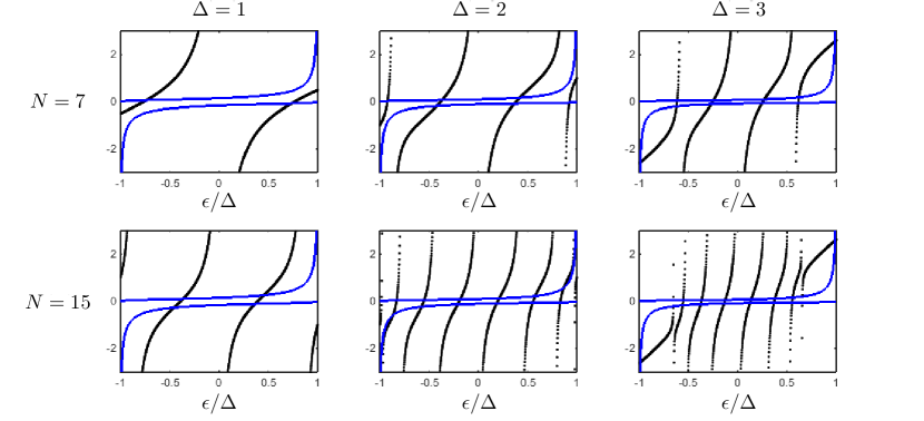
Figure 3: (Color online) Bound modes of an SNS junction. The figure shows plots of two independent constraints derived from the boundary matrix against the ratio $\epsilon/\Delta$, as energy is swept from $-\Delta$ to $\Delta$ (with reference to Appendix C, these constraints are the functions on the left hand-side (blue solid lines) and right hand-side (black dotted lines) of Eq. (43) and Eq. (43b). Each intersection of the two distinct sets of lines indicates the emergence of a bound state. The plots in the top (bottom) panels correspond to $N=7$ ($N=15$), respectively. Parameters $t=1,t^{\prime}=0.5$ are fixed for all the plots. The number of intersections shows an expected increment as we increase the length of the normal region (N) from $N=7$ to $15$, without changing other parameters. For a fixed value of $N$, the number of intersections increases as we change $\Delta=1$ to $\Delta=2$, but it stays constant for $\Delta=2$ vs. $\Delta=3$, except for additional states pinned to the energies near $\epsilon=\pm\Delta$.

III.2 Application to SNS junctions

We illustrate the generalized Bloch theorem for interfaces by outlining an analytical calculation of the Andreev bound states for an idealized SNS junction. The equilibrium Josephson effect, namely, the phenomenon of supercurrent flowing through a junction of two superconducting leads connected via a normal link, is of great importance for theoretical understanding of superconductivity, as well as for its applications in SC circuits. One of the questions this phenomenon poses is to understand how exactly a weak link with induced band-gap due to superconducting proximity effect can carry a supercurrent. An answer to this question invokes the formation of bound states in the band gap of the weak link, known as the “Andreev bound states”, that allow transport of Cooper pairs lesovik11 .

We model a basic $D=1$ SNS junction as a system formed by attaching a finite metallic chain (a “normal dot”, denoted by N) to two semi-infinite SC chains (“superconducting leads”, denoted by S1 and S2). Following Ref. [bena12, ], we describe the SC leads in terms of a $D=1$ BCS pairing Hamiltonian,

$$\widehat{H}_{\sf S}=-\sum_{j,\sigma}tc^{\dagger}_{j\sigma}c_{j+1\sigma}-\sum_{j}\Delta c_{j\uparrow}^{\dagger}c_{j\downarrow}^{\dagger}+\text{H.c.},$$ (20)

where we have assumed zero chemical potential. This Hamiltonian can be diagonalized analytically for open BCs, see Appendix B (see also Refs. [arutyunov08, ; ortiz14, ; ortiz16, ] for a critical discussion of $D=1$ models of superconductivity). The normal dot is modeled by NN hopping of strength $t$. The links connecting the SC regions to the metallic one have a weaker hopping strength, $t^{\prime}<t$. The Hamiltonian of the full system is thus $\widehat{H}_{\sf SNS}=\widehat{H}_{\sf S1}+\widehat{H}_{\sf S2}+\widehat{H}_{\sf T}+\widehat{H}_{\sf N},$ where $\widehat{H}_{\sf S1}$ and $\widehat{H}_{\sf S2}$ denote the SC Hamiltonians for the leads, $\widehat{H}_{\sf N}$ describes the normal metal, and $\widehat{H}_{\sf T}$ is the tunneling Hamiltonian, of the form

$$\widehat{H}_{\sf T}=-\!\!\sum_{\sigma=\pm 1}[t^{\prime}(c_{-2{\sf L}\sigma}^{\dagger}c_{-2{\sf L}+1\sigma}+c_{2{\sf L}-1\sigma}^{\dagger}c_{2{\sf L}\sigma})+\text{H.c.}].$$ (21)

The region S1 extends from $j=-\infty$ on the left to $j=-2{\sf L}$, whereas S2 extends from $j=2{\sf L}$ to $j=\infty$, so that the length the of the metallic chain is $N\equiv 4{\sf L}-1$.

The technical implementation of our diagonalization procedure for junctions is described in full detail in Appendix C. Let us summarize the key results here (see also Fig. 3 for illustration). The structure of the boundary equations makes clear the dependence of the number of bound states with the length $N$ of the normal dot and the pairing amplitude $\Delta$. When the metal strip is completely disconnected from the SC, that is, when $t^{\prime}=0$, the stationary states of the normal dot (standing waves) are labelled by the quantum numbers $k=\frac{\pi q}{2{\sf L}}+\frac{\pi}{4{\sf L}},$ $q=0,1,\dots,2{\sf L}-1$, typical of the lattice-regularized infinite square well. Each of these states at energy less than $\Delta$ turns into a bound state with a slightly different value of energy for weak tunneling. For a fixed value of $\Delta$, increasing $N$ allows for more solutions of the boundary equations, and so for more Andreev bound states. Conversely, for fixed $N$ the number of bound modes does not increase with the value of $\Delta$ once $|\Delta|>|t|$. Instead, we find pinning of bound states near energy values $\epsilon=\pm\Delta$ as $N$ increases. These pinned states, that appear only if $|\Delta|>|t|$, are characterized physically by a large penetration depth in the superconducting regions S1 and S2.

IV Surface bands in higher-dimensional systems

In this section we illustrate the application of the generalized Bloch theorem to computing surface bands. Our goal is to gain as much insight as possible on the interplay between bulk properties – topological or otherwise – and BCs toward establishing the structure of surface bands. We consider first a prototypical ladder system, the Creutz ladder Creutz , as a stepping stone going from one dimension to two. We next examine a graphene ribbon, partly because there has been a considerable amount of analytical work on the surface band structure of this system. Thus, this permits benchmarking our generalized Bloch theorem against other approaches. In this regard, we emphasize that our method yields analytically all of the eigenstates and eigenvalues of a graphene strip, not just the surface ones.

Our two final illustrative systems are $D=2$ TSCs. Specifically, we first compute the surface band structure of the chiral $p+ip$ TSC analytically, with emphasis on the interplay between the phase diagram of the lattice model and its surface physics. A key point here is to gain physical insight into the emergence of chiral surface bands from the point of view of the boundary matrix. We conclude by providing an exact, albeit non analytical, solution for the Majorana surface flat bands of a time-reversal invariant gapless $s$-wave TSC model. Here, we both revisit the anomalous bulk-boundary correspondence that this model is known to exhibit Deng14 through the eyes of the boundary matrix, and leverage access to the system’s eigenstates to characterize physical equilibrium properties. Notably, we predict that the presence of a Majorana surface flat band implies a substantial enhancement in the equilibrium $4\pi$-periodic Josephson supercurrent as compared to a gapped $D=2$ TSC that hosts only a finite number of Majorana modes.

IV.1 The Creutz ladder

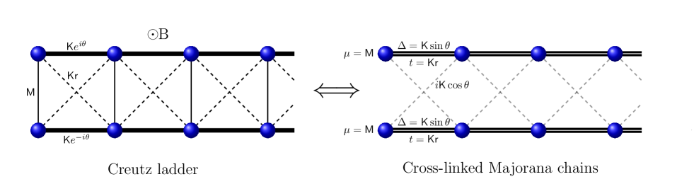
Figure 4: (Color online) Schematic of the duality between the Creutz ladder (left) and cross-linked Majorana chains (right).

The ladder model described by Hamiltonian

$$\widehat{H}= -\sum_{j}\big{[}{\sf K}(e^{i\theta}a_{j}^{\dagger}a_{j+1}+e^{-i\theta}b_{j}^{\dagger}b_{j+1}+\text{H.c.})+$$

$$+{\sf r}{\sf K}(a_{j}^{\dagger}b_{j+1}+b_{j}^{\dagger}a_{j+1}+\text{H.c.})+{\sf M}(a_{j}^{\dagger}b_{j}+b_{j}^{\dagger}a_{j})\big{]}.$$ (22)

is typically referred to as the Creutz ladder after its proponent Creutz ; CreutzRMP ; CreutzPRD , and is schematically depicted in Fig. 4(left). Here, $a_{j}$ and $b_{j}$ denote fermionic annihilation operators for fermions at site $j$ of two parallel chains visualizable as the sides of a ladder. Fermions on each side of the ladder are characterized by an inverse effective mass ${\sf K}$. There is a homogeneous magnetic field perpendicular to the plane of the ladder, responsible for the phase $e^{i\theta}$($e^{-i\theta}$) for hopping along the upper (lower) side of the ladder. Hopping along rungs of the ladder occur with amplitude ${\sf M}$, whereas diagonal hoppings occur with amplitude ${\sf K}{\sf r}$.

The Creutz ladder is known to host mid-gap bound states when $|{\sf M}|<|2{\sf K}{\sf r}|$ and $\theta\neq 0,\pi$. Such states are called domain-wall fermions in lattice quantum field theory. The domain-wall fermions of the Creutz ladder are, for the most part, not topologically protected or mandated by the bulk-boundary correspondence. If $\theta\neq\pm\pi/2$, the Creutz ladder may be classified as a $D=1$ model in class $A$, thus the domain-wall fermions are not protected. However, if $\theta=\pm\pi/2$, then the Creutz ladder enjoys a chiral symmetry, and with a canonical transformation of the fermionic basis, the single-particle Hamiltonian can be made real (see Appendix  D). In this parameter regime, the model belongs to class BDI, which is topologically non-trivial in $D=1$. Interestingly, this was the parameter regime analyzed in depth in the original work Creutz . We reveal some of these features analytically for ${\sf r}=\pm 1$ in Appendix D. Ladder systems are not quite $D=1$, but are not $D=2$ either. Ultimately, it is more convenient to investigate ladders in terms of the basic generalized Bloch theorem of Part I. For this reason, we have chosen to relegate a detailed discussion of the diagonalization of the Creutz ladder to Appendix D. In the following, we highlight two related new results: a many-body duality transformation that maps the Creutz ladder to a pair of Majorana chains, and the existence of edge modes with a power-law prefactor.

IV.1.1 The dual Majorana ladder

The Gaussian duality transformation equivalence

$$a_{j}\mapsto\mathcal{U}_{\sf d}a_{j}\mathcal{U}_{\sf d}^{\dagger}={\sf c}\,a_{j}+i{\sf s}\,a_{j}^{\dagger}-i{\sf c}\,b_{j}+{\sf s}\ b_{j}^{\dagger},$$

$$b_{j}\mapsto\mathcal{U}_{\sf d}b_{j}\mathcal{U}_{\sf d}^{\dagger}={\sf s}\,a_{j}-i{\sf c}\,a_{j}^{\dagger}-i{\sf s}\,b_{j}-{\sf c}\ b_{j}^{\dagger},$$

with $\mathcal{U}_{\sf d}$ a unitary transformation in Fock space and (${\sf c}=\frac{\cos\varphi}{\sqrt{2}}$, ${\sf s}=\frac{\sin\varphi}{\sqrt{2}}$), transforms the Creutz ladder model to a dual SC. Specialized to $\varphi=\pi/4$, the dual SC Hamiltonian is $\mathcal{U}_{\sf d}\widehat{H}\mathcal{U}_{\sf d}^{\dagger}=\widehat{H}_{a}+\widehat{H}_{b}+\widehat{H}_{ab}$, with

$$\widehat{H}_{a}=\!-\sum_{j}\big{[}ta_{j}^{\dagger}a_{j+1}+\frac{\mu}{2}a_{j}^{\dagger}a_{j}+\Delta\,a_{j}a_{j+1}+\text{H.c.}],$$

$$\widehat{H}_{b}=\!-\sum_{j}\big{[}tb_{j}^{\dagger}b_{j+1}+\frac{\mu}{2}b_{j}^{\dagger}b_{j}+\Delta\,b_{j}b_{j+1}+\text{H.c.}],$$

$$t \equiv{\sf r}{\sf K},\quad\Delta\equiv{\sf K}\sin\theta,\quad\mu\equiv{\sf M},$$

and, finally,

$$\widehat{H}_{ab}=\!-\sum_{j}\big{[}i{\sf K}\cos\theta(b^{\dagger}_{j}a_{j+1}+b^{\dagger}_{j+1}a_{j}-\text{H.c.})-{\sf M}\big{]}.$$

We conclude that the dual system may be described as a ladder consisting of Majorana chains on each side, connected by electron tunneling and with no pairing term associated to the rungs of the ladder [see Fig. 4(right)]. Moreover, the Majorana chains (the sides of the ladder) decouple if $\theta=\pm\pi/2$, in which case the Creutz ladder displays chiral symmetry. Since these two decoupled Majorana chains have real parameter values, the dual system also belongs to the topologically non-trivial class D.

The fermion number operator $\hat{N}_{F}\equiv\sum_{j}(a_{j}^{\dagger}a_{j}+b_{j}^{\dagger}b_{j})$, regarded as the broken particle conservation symmetry of the Majorana ladder, maps by the inverse of the duality transformation to a broken symmetry $\hat{N}_{C}\equiv\mathcal{U}^{\dagger}_{\sf d}\hat{N}_{F}\mathcal{U}_{\sf d}$ of the Creutz ladder. In other words, we expect the insulating spectral gap of the Creutz ladder to close whenever the symmetry $\hat{N}_{C}$ is restored, unless there is a stronger factor at play. This symmetry is restored for ${\sf K}\sin(\theta)=0$, which is indeed a gapless regime unless ${\sf K}=0$, because then the Creutz ladder reaches the atomic limit. A similar explanation of the insulating gap for the Peierls chain in terms of a hidden broken symmetry was given in Ref. [equivalence, ], where fermionic Gaussian dualities were investigated in higher dimensions as well.

IV.1.2 Topological power-law modes

The generalized Bloch theorem identifies regimes in which the domain-wall fermions of the Creutz ladder may display power-law behavior. From the analysis in Appendix D, power-law modes are forbidden only if ${\sf M}=0,$ $\theta=\pm\pi/2$ and ${\sf K}\neq 0,$ ${\sf r}\neq\pm 1$. For arbitrary values of ${\sf K},{\sf r},\theta,{\sf M}$, one can expect in general a finite number of values of $\epsilon$ for which the full solution of the bulk equation includes power-law modes, potentially compatible with the BCs. Let us point out for illustration the power-law modes of the Creutz ladder in the parameter regime $\theta=\pi/2,\ {\sf M}=2{\sf K}\sqrt{{\sf r}^{2}-1}$, with ${\sf r}>1$. In this regime the Creutz ladder is dual to two decoupled Kitaev chains, each individually on its “circle of oscillations” in its phase diagram hegde16 . The topological power-law modes of the Kitaev chain have been explicitly described in Part I (see Sec. V C). Therefore, the power-law topological edge modes of the Creutz ladder may be found by way of our duality transformation. Alternatively, there is a shortcut at the single-particle level.

Let us rewrite the Creutz ladder in terms of a new set of fermionic degrees of freedom

$$\widetilde{a}_{j}=\frac{1}{\sqrt{2}}(a_{j}+b_{j}),\quad\widetilde{b}_{j}=\frac{i}{\sqrt{2}}(a_{j}-b_{j}).$$ (23)

Unlike for our previous duality transformation, the result is another particle-conserving Hamiltonian. The associated single-particle Hamiltonian is

$$\widetilde{H}_{N}=\mathds{1}_{N}\otimes\tilde{h}_{0}+T\otimes\tilde{h}_{1}+T^{\dagger}\otimes\tilde{h}_{1}^{\dagger},$$ (24)

$$\tilde{h}_{0}=-\begin{bmatrix}{\sf M}&0\\ 0&-{\sf M}\end{bmatrix},$$

$$\tilde{h}_{1}=-\begin{bmatrix}{\sf K}({\sf r}+\cos\theta)&{\sf K}\sin\theta\\ -{\sf K}\sin\theta&{\sf K}(-{\sf r}+\cos\theta)\end{bmatrix}.$$

For $\theta=\pi/2$, and with the identifications $t={\sf K}{\sf r},\Delta={\sf K}\sin\theta,\mu={\sf M}$ already introduced, the above $\widetilde{H}_{N}$ becomes identical to the single-particle Hamiltonian for the Majorana chain of Kitaev. Moreover, if ${\sf M}=\mu=2{\sf K}\sqrt{{\sf r}^{2}-1}$, it follows that $(\mu/2t)^{2}+(\Delta/t)^{2}=1$. This is the aforementioned coupling regime known as the “circle of oscillations”. Hence, by simply translating the calculations of Part I, Sec. V C, we obtain the topological power-law mode

$$|\epsilon=0\rangle=\sum_{j=1}^{\infty}j\,w^{j-1}|j\rangle\begin{bmatrix}1\\ -1\end{bmatrix},\quad w\equiv-\Big{(}\frac{{\sf r}-1}{{\sf r}+1}\Big{)}^{1/2},$$

of the Creutz ladder (in the particle-conserving representation of Eq. (23)). To our knowledge, this provides the first example of a topological power-law zero mode in a particle-conserving Hamiltonian in class AIII.

IV.2 Graphene ribbons

In this section we investigate NN tight-binding models on the honeycomb (hexagonal) lattice, with graphene as the prime motivation castroneto09 . The surface band structure of graphene sheets or ribbons is well understood, even analytically in limiting cases mao10 ; kohmoto07 ; delplace11 ; Iachello . As emphasized in Ref. [yao09, ], a perturbation that breaks inversion symmetry can have interesting effects on these surface bands. With this in mind, in our analysis below we include a sublattice potential and show that the Hamiltonian for a ribbon subject to zigzag-bearded BCs can be fully diagonalized in closed form.

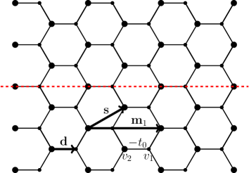
Figure 5: (Color online) Graphene ribbon, periodic or infinite in the horizontal ${\mathbf{m}}_{1}$ direction. Left: The ribbon is terminated in the vertical direction by a zigzag edge on the bottom and a “bearded” edge on top. The decoupled $B$ sites at the top are auxiliary degrees of freedom. Right: The ribbon is terminated by armchair edges. The system has mirror symmetry about the dashed (red) line. In both cases, on-site potentials $v_{1}$ and $v_{2}$ are associated with the $A$ and $B$ sublattice, respectively.

IV.2.1 Zigzag-bearded boundary conditions

The honeycomb lattice is bipartite, with triangular sublattices $A$ and $B$ displaced by ${\mathbf{d}}$ relative to each other, see Fig. 5(left). We parametrize the lattice sites $\mathbf{R}$ as

$$\mathbf{R}(j_{1},j,m)=\left\{\begin{array}[]{lcl}j_{1}{\mathbf{m}}_{1}+j{\mathbf{s}}+{\mathbf{d}}&\mbox{if}&m=1\\ j_{1}{\mathbf{m}}_{1}+j{\mathbf{s}}&\mbox{if}&m=2\end{array}\right.,\quad$$

$${\mathbf{m}}_{1}\equiv a\begin{bmatrix}1\\ 0\end{bmatrix},\ {\mathbf{s}}=\frac{a}{2}\begin{bmatrix}1\\ \sqrt{3}\end{bmatrix},\ {\mathbf{d}}=-\frac{a}{2\sqrt{3}}\begin{bmatrix}\sqrt{3}\\ 1\end{bmatrix},$$

with $j_{1},j\in\mathds{Z}$, $a=1$ being the lattice parameter and $m=1$ ($m=2$) denoting the $A$ ($B$) sublattice. The localized (basis) states are $|{\mathbf{j}}\rangle|m=1\rangle$ and $|{\mathbf{j}}\rangle|m=2\rangle$, and so the sublattice label plays the role of a pseudospin-$1/2$ degree of freedom. The ribbon we consider is translation-invariant in the ${\mathbf{m}}_{1}$ direction and terminated along ${\mathbf{s}}$, with single-particle Hamiltonian $H_{N}=\sum_{{\mathbf{k}}_{\parallel}\in\text{SBZ}}|{\mathbf{k}}_{\parallel}\rangle\langle{\mathbf{k}}_{\parallel}|\otimes H_{{\mathbf{k}}_{\parallel},N}$, where

$$H_{{\mathbf{k}}_{\parallel},N} = \mathds{1}_{N}\otimes\begin{bmatrix}v_{1}&-t_{0}(1+e^{-ik_{\parallel}})\\ -t_{0}(1+e^{ik_{\parallel}})&v_{2}\end{bmatrix}$$

$$+ \Big{(}T\otimes\begin{bmatrix}0&0\\ -t_{0}&0\end{bmatrix}+\text{H.c.}\Big{)},$$

and the $2\times 2$ matrices act on the sublattice degree of freedom. Notice that $H_{N}$ is chirally symmetric if the on-site potentials $v_{1}=0=v_{2}$, and the edges of the ribbon are of the zigzag type, see Fig. 5(left). While in the following we shall set $v_{1}=0$ for simplicity, it is easy to restore $v_{1}$ anywhere along the way if desired. In particular, $v_{1}=-v_{2}$ is an important special case yao09 .

The analytic continuation of the Bloch Hamiltonian is

$$H_{k_{\parallel}}(z)=\begin{bmatrix}0&-t_{1}(k_{\parallel})e^{-i\phi_{k_{\parallel}}}-t_{0}z^{-1}\\ -t_{1}(k_{\parallel})e^{i\phi_{k_{\parallel}}}-t_{0}z&v_{2}\end{bmatrix},$$

$$t_{1}(k_{\parallel})\equiv t_{0}\sqrt{2(1+\cos(k_{\parallel}))},\ \ e^{i\phi_{k_{\parallel}}}\equiv t_{0}(1+e^{ik_{\parallel}})/t_{1}(k_{\parallel}).$$

This analysis reveals the formal connection between graphene and the Su-Schrieffer-Heeger (SSH) model: just compare the above $H_{k_{\parallel}}(z)$ with $H(z)$ in Eq. (55).

We impose BCs in terms of an operator $W$ such that

$$\langle k_{\parallel}|W|k_{\parallel}^{\prime}\rangle\!=\!\delta_{k_{\parallel},k_{\parallel}^{\prime}}|N\rangle\langle N|\otimes\begin{bmatrix}0&t_{1}(k_{\parallel})e^{-i\phi_{k_{\parallel}}}\\ t_{1}(k_{\parallel})e^{i\phi_{k_{\parallel}}}&0\end{bmatrix}.$$

In real space, this corresponds to

$$W=\, \mathbf{1}\otimes|N\rangle\langle N|\otimes\begin{bmatrix}0&-t_{0}\\ -t_{0}&0\end{bmatrix}+$$

$$\quad\quad\quad+\Big{(}\mathbf{T}\otimes|N\rangle\langle N|\otimes\begin{bmatrix}0&0\\ -t_{0}&0\end{bmatrix}+\text{H.c.}\Big{)},$$

The meaning of these BCs is as follows: for the modified ribbon Hamiltonian described by $H=H_{N}+W$, the sites $|j_{1}\rangle|j=N\rangle|B\rangle$ are decoupled from the rest of the system and each other, see Fig. 5(left). The termination of the actual ribbon, consisting of the sites connected to each other, is of the zigzag type on the lower edge, and “bearded” on the upper edge. From a geometric perspective, this ribbon is special because every $B$ site is connected to exactly three $A$ sites, but not the other way around.

At this point we may borrow results from dimerized chains that we include in Appendix  E, to which we refer for full detail. The energy eigenstates that are perfectly localized on the upper edge (consisting of decoupled sites) constitute a flat surface band at energy $v_{2}$. For $|k_{\parallel}|>2\pi/3$, the energy eigenstates localized on the lower edge constitute a flat surface band at $v_{1}=0$ energy. Explicitly, these zero modes are

$$|\epsilon=0,k_{\parallel}\rangle= |k_{\parallel}\rangle|z_{1}(k_{\parallel})\rangle\begin{bmatrix}(t_{1}(k_{\parallel})^{2}-t_{0}^{2})e^{-i\phi_{k_{\parallel}}}/t_{1}(k_{\parallel})\\ 0\end{bmatrix},$$

$$\quad z_{1}(k_{\parallel})\equiv -e^{i\phi_{k_{\parallel}}}\frac{t_{1}(k_{\parallel})}{t_{0}}=-(1+e^{ik_{\parallel}}).$$

While their energy is insensitive to $k_{\parallel}$, their characteristic localization length is not; specifically,

$$\ell_{\rm loc}(k_{\parallel})=-\frac{1}{\ln(|z_{1}(k_{\parallel})|)}=-\frac{2}{\ln(2+2\cos(k_{\parallel}))}.\quad$$ (25)

For $k_{\parallel}\neq\pm\frac{2\pi}{3}$, the bulk states are

$$|\epsilon_{n}(k_{\parallel},q)\rangle\!=\!|k_{\parallel}\rangle|\chi_{1}(q)\rangle\!\begin{bmatrix}t_{1}(k_{\parallel})e^{-i\phi_{k_{\parallel}}}\\ -\epsilon_{n}(k_{\parallel},q)\end{bmatrix}\!+\!|k_{\parallel}\rangle|\chi_{2}(q)\rangle\!\begin{bmatrix}t_{0}\\ 0\end{bmatrix},$$

with

$$|\chi_{1}(q)\rangle\equiv 2i\sum_{j=1}^{N}\sin\!\big{(}\pi qj/N\big{)}e^{-i\phi j}|j\rangle,$$ (26)

$$|\chi_{2}(q)\rangle\equiv 2i\sum_{j=1}^{N}\sin\!\big{(}\pi q(j-1)/N\big{)}e^{-i\phi(j-1)}|j\rangle,$$ (27)

$$\epsilon_{n}(k_{\parallel},q)=$$ (28)

$$=\frac{v_{2}}{2}+(-1)^{n}\sqrt{\frac{v_{2}^{2}}{4}+t_{1}(k_{\parallel})^{2}+t_{0}^{2}+2t_{1}(k_{\parallel})t_{2}\cos\!\big{(}\frac{\pi}{N}q\big{)}},$$

for $n=1,2$. Since $t_{1}(k_{\parallel}=\pm\frac{2\pi}{3})=t_{0}$, the virtual chains $H_{k_{\parallel},N}$ are gapless if $v_{2}=0$, reflecting the fact that graphene is a semimetal. The energy eigenstates are similar but simpler than the ones just described.

IV.2.2 Armchair terminations

The graphene ribbon with zigzag terminations can be described in terms of smooth terminations of the triangular Bravais lattice with two atoms per unit cell. In contrast, armchair terminations require a fairly different description of the underlying atomic array. Figure 5(right) shows how to describe this system in terms of a centered rectangular Bravais lattice bechstedt with two atoms per unit cell and smooth parallel terminations. In this case, we parametrize the lattice sites $\mathbf{R}$ as

$$\mathbf{R}(j_{1},j,m)=\left\{\begin{array}[]{lcl}j_{1}{\mathbf{m}}_{1}+j{\mathbf{s}}+{\mathbf{d}}&\mbox{if}&m=1\\ j_{1}{\mathbf{m}}_{1}+j{\mathbf{s}}&\mbox{if}&m=2\end{array}\right.,$$

$${\mathbf{m}}_{1}\equiv a\begin{bmatrix}\sqrt{3}\\ 0\end{bmatrix},\ {\mathbf{s}}=\frac{a}{2}\begin{bmatrix}\sqrt{3}\\ 1\end{bmatrix},\ {\mathbf{d}}=\frac{a}{\sqrt{3}}\begin{bmatrix}1\\ 0\end{bmatrix},$$

where as before $j_{1},j\in\mathds{Z}$, $a=1$, and $m\in\{1,2\}$ labels the sublattice. The total single-particle Hamiltonian can now be taken to read $H=H_{N}+W$, with $W=0$ and $H_{N}=\sum_{{\mathbf{k}}_{\parallel}\in\text{SBZ}}|{\mathbf{k}}_{\parallel}\rangle\langle{\mathbf{k}}_{\parallel}|\otimes H_{{\mathbf{k}}_{\parallel},N}$, where

$$H_{{\mathbf{k}}_{\parallel},N}=\mathds{1}_{N}\otimes\begin{bmatrix}v_{1}&-t_{0}\\ -t_{0}&v_{2}\end{bmatrix}+\Big{(}T\otimes\begin{bmatrix}0&-t_{0}e^{-ik_{\parallel}}\\ -t_{0}&0\end{bmatrix}+\text{H.c.}\Big{)},$$

and the analytic continuation of the Bloch Hamiltonian for each $k_{\parallel}$ is

$$H_{k_{\parallel}}(z)\!=\!\begin{bmatrix}v_{1}&-t_{0}(1+ze^{-ik_{\parallel}}+z^{-1})\\ -t_{0}(1+z^{-1}e^{ik_{\parallel}}+z)&v_{2}\end{bmatrix}.$$

The diagonalization of the Hamiltonian proceeds from here on as before. There is, however, a shortcut based on Appendix A, which explains in addition the absence of edge modes in this system. Let $T_{k_{\parallel}}\equiv e^{-ik_{\parallel}/2}T$. In terms of this $k_{\parallel}$-dependent matrix,

$$H_{{\mathbf{k}}_{\parallel},N}\!=\!\mathds{1}_{N}\otimes\begin{bmatrix}v_{1}&\!\!-t_{0}\\ -t_{0}&\!\!v_{2}\end{bmatrix}-t_{0}\Big{(}T_{k_{\parallel}}+T_{k_{\parallel}}^{\dagger}\Big{)}\otimes\begin{bmatrix}0&e^{-ik_{\parallel}/2}\\ e^{ik_{\parallel}/2}&0\end{bmatrix}\!.$$

It follows that the (unnormalized) energy eigenstates of the graphene ribbon with armchair terminations are

$$|\epsilon_{q,\pm}\rangle=|k_{\parallel}\rangle\sum_{j=1}^{N}|j\rangle e^{ik_{\parallel}j/2}\sin[\pi qj/(N+1)]\begin{bmatrix}-2t_{0}(1+e^{-ik_{\parallel}/2}\cos[\pi q/(N+1)])\\ \epsilon_{q,\pm}\end{bmatrix},\qquad q=1,\dots,N,$$

where $\epsilon_{q,+}$ and $\epsilon_{q,-}$ are the two roots (in $\epsilon$) of the quadratic equation

$$\epsilon^{2}-v_{2}\epsilon-t_{0}^{2}-4t_{0}^{2}\cos(k_{\parallel}/2)\cos[\pi q/(N+1)]-4t_{0}^{2}\cos^{2}[\pi q/(N+1)]=0.$$

These are the $2N$ energy eigenstates of the system for each value of $k_{\parallel}$.

IV.3 A chiral $p+ip$ superconductor

The spinless $p+ip$ SC of Ref. [read00, ] is the prototype of spinless superconductivity in $D=2$. The model may be regarded as the mean-field approximation to an exactly-solvable (by the algebraic Bethe ansatz) pairing Hamiltonian rombouts10 . It belongs to class D in the Altland-Zirnbauer classification, and thus, according to the ten-fold way, it admits an integer ($\mathbb{Z}$) topological invariant. There has been hope for some time that the related phenomenon of triplet superconductivity is realized in layered perovskite strontium ruthenate $\rm Sr_{2}RuO_{4}$, but the matter remains controversial Sr2RuO4 . The many-body model Hamiltonian can be taken to be

$$\hat{H}=-t\sum_{{\mathbf{r}}}(c_{{\mathbf{r}}+{\mathbf{s}}}^{\dagger}c_{{\mathbf{r}}}+c_{{\mathbf{r}}+{\mathbf{m}}}^{\dagger}c_{{\mathbf{r}}}+\text{H.c.})$$

$$-\Delta\sum_{{\mathbf{r}}}(c_{{\mathbf{r}}}c_{{\mathbf{r}}+{\mathbf{s}}}-ic_{{\mathbf{r}}}c_{{\mathbf{r}}+{\mathbf{m}}}+\text{H.c.})-(\mu-4t)\sum_{\mathbf{r}}c^{\dagger}_{\mathbf{r}}c_{\mathbf{r}},$$

on the square lattice of unit lattice spacing and with standard unit vectors ${\mathbf{s}},{\mathbf{m}}$ pointing in the $x$ and $y$ directions, respectively. The parameters $t,\Delta$ are real numbers. The corresponding single-particle Hamiltonian is

$$H =-[(\mu-4t)\mathds{1}+t(T_{\mathbf{s}}+T_{\mathbf{s}}^{\dagger})+t(T_{\mathbf{m}}+T_{\mathbf{m}}^{\dagger})]\otimes\tau_{z}+$$

$$+i\Delta(T_{\mathbf{s}}-T_{\mathbf{s}}^{\dagger})\otimes\tau_{y}+i\Delta(T_{\mathbf{m}}-T_{\mathbf{m}}^{\dagger})\otimes\tau_{x},$$

in terms of shift operators $T_{\mathbf{s}}\equiv\sum_{\mathbf{r}}|{\mathbf{r}}\rangle\langle{\mathbf{r}}+{\mathbf{s}}|,$ $T_{\mathbf{m}}\equiv\sum_{\mathbf{r}}|{\mathbf{r}}\rangle\langle{\mathbf{r}}+{\mathbf{m}}|$ which can be adjusted to describe relevant BCs (open-open, open-periodic, periodic-open, and periodic-periodic).

IV.3.1 Closed-form chiral edge states

If energy is measured in units of $t$, then the parameter space of the model can be taken to be two-dimensional after a gauge transformation that renders $\Delta>0$. We shall focus on the line $\Delta=1=t$, in which $\mu$ is the only variable parameter. The Bloch Hamiltonian is

$$H({\mathbf{k}}) =\begin{bmatrix}e({\mathbf{k}})&\Delta({\mathbf{k}})\\ \Delta({\mathbf{k}})^{*}&-e({\mathbf{k}})\end{bmatrix},$$

$$\Delta({\mathbf{k}}) \equiv 2i\sin k_{1}-2\sin k_{2},$$

$$e({\mathbf{k}}) \equiv-2\cos k_{1}-2\cos k_{2}-\mu+4,$$

for ${\mathbf{k}}=(k_{1},k_{2})\in[-\pi,\pi)\times[-\pi,\pi)$. The resulting single-particle bulk dispersion then reads

$$\epsilon(k_{1},k_{2})^{2} = \mu^{2}-8\mu+24+4(\mu-4)(\cos k_{1}+\cos k_{2})$$

$$+ 8\cos k_{1}\cos k_{2},$$

and it is fully gapped unless $\mu=0,4,8$. The gap closes at ${\mathbf{k}}=0$ if $\mu=0$, ${\mathbf{k}}=(-\pi,0)$ and ${\mathbf{k}}=(0,-\pi)$ if $\mu=4$, and at ${\mathbf{k}}=(-\pi,-\pi)$ if $\mu=8$. For $0<\mu<8$, the system is in the weak-pairing topologically non-trivial phase with odd fermion number parity in the ground state. The phase transition to the trivial strong-pairing phase happens at $\mu=0$ read00 .

We now impose open BCs in the $x$ direction while keeping the $y$ direction translation invariant, that is, $k_{2}=k_{\parallel}$. Accordingly, we need the analytic continuation of the Bloch Hamiltonian in $k_{1}$. Let us introduce the compact notation

$$\omega\equiv-2\cos k_{\parallel}-\mu+4,\quad\xi\equiv-2\sin k_{\parallel},$$

so that $H_{k_{\parallel}}(z)=h_{k_{\parallel},0}+zh_{1}+z^{-1}h_{1}^{\dagger}$, with

$$h_{k_{\parallel},0}=\begin{bmatrix}\omega&\xi\\ \xi&-\omega\end{bmatrix},\quad h_{1}=\begin{bmatrix}-1&1\\ -1&1\end{bmatrix}.$$ (29)

The condition $\det(H_{k_{\parallel}}(z)-\epsilon\mathds{1}_{2})=0$ is then equivalent to the equation

$$\epsilon^{2} =\omega^{2}+\xi^{2}+4-2\omega\,(z+z^{-1}).$$ (30)

Note that the replacement $z+z^{-1}\mapsto 2\cos k_{1}$ recovers the bulk dispersion relation. Moreover, if $2<\mu<6$, there are values of $k_{\parallel}$ for which $\omega=0$ and the dispersion relation becomes flat. From $H_{k_{\parallel}}(z)$ it is immediate to reconstruct the family of virtual chain Hamiltonians

$$H_{k_{\parallel},N} =\mathds{1}_{N}\otimes h_{k_{\parallel},0}+T\otimes h_{1}+T^{\dagger}\otimes h_{1}^{\dagger}.$$

From the point of view of any one of these chains, mirror symmetry is broken by the NN pairing terms. This fact is important, because then the boundary matrix is not mirror-symmetric either, which will ultimately lead to surface states of opposite chirality on the left and right edges.

The number of edge degrees of freedom is $2Rd=4$ for each value of $k_{\parallel}$. Since $h_{1}$ [Eq. (29)] is not invertible, and Eq. (30) is a polynomial of degree $2$ in $z$, the complete eigenstate ansatz is formed out of four independent states (one ansatz state for each $k_{\parallel}$): two extended states associated to the roots $z_{\ell}=z_{\ell}(\epsilon,k_{\parallel}),$ $\ell=1,2,$ of Eq. (30), and two emergent states of finite support localized on the edges of the virtual chains $H_{k_{\parallel},N}$. With hindsight, we will ignore the emergent states and focus on the reduced ansatz, namely,

$$|\epsilon\rangle=\alpha_{1}|z_{1},1\rangle|u_{1}\rangle+\alpha_{2}z_{2}^{-N+1}|z_{2},1\rangle|u_{2}\rangle.$$

The state $|z_{1},1\rangle|u_{1}\rangle$ should represent a surface state for the left edge, $z_{2}^{-N+1}|z_{2},1\rangle|u_{2}\rangle$ one for the right edge, with

$$|u_{\ell}\rangle=\begin{bmatrix}\xi+z_{\ell}-z_{\ell}^{-1}\\ -\omega+\epsilon+z_{\ell}+z_{\ell}^{-1}\end{bmatrix}$$ (31)

satisfying the equation $H_{k_{\parallel}}(z_{\ell})|u_{\ell}\rangle=\epsilon|u_{\ell}\rangle$. The boundary equations $P_{\partial}(H_{k_{\parallel},N}-\epsilon\mathds{1}_{2N})|\epsilon\rangle=0$ are encoded in the boundary matrices

$$B_{k_{\parallel}}(\epsilon)=-\begin{bmatrix}h_{1}^{\dagger}|u_{1}\rangle&z_{2}^{-N-1}h_{1}^{\dagger}|u_{2}\rangle\\ z_{1}^{N+1}h_{1}|u_{1}\rangle&h_{1}|u_{2}\rangle\end{bmatrix},$$

which are, however, non-square $4\times 2$ matrices as we have ignored the two emergent states that in principle appear in the ansatz. Nonetheless, since $h_{1}$ is a matrix of rank one, we can extract a square boundary matrix, namely,

$$\tilde{B}_{k_{\parallel}}(\epsilon)\!=\!\begin{bmatrix}z_{1}(\xi-\omega+\epsilon+2z_{1})&\!z_{2}^{-N}(\xi-\omega+\epsilon+2z_{2})\\ z_{1}^{N}(\xi+\omega-\epsilon-2z_{1}^{-1})&\!z_{2}(\xi+\omega-\epsilon-2z_{2}^{-1})\end{bmatrix},$$

that properly captures the BCs for our reduced trial states. Surface states are characterized by the condition $|z_{1}|=|z_{2}^{-1}|<1$. Hence, in the large-$N$ limit, one may set $z_{1}^{N}=z_{2}^{-N}=0$. Within this approximation, the left and right edges are effectively decoupled by virtue of their large spatial separation.

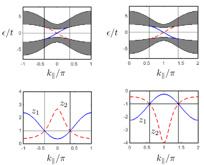
Figure 6: (Color online) Surface bands for $\mu=1.5$, centered at $k_{\parallel}=0$ (top left panel), and $\mu=6.5$, centered at $k_{\parallel}=-\pi$ (top right panel). The shaded (gray) region shows the bulk bands. The electrons on the right edge (dashed red curve) propagate to the right only, and those on the left edge (solid blue curve) to the left only, that is, the surface bands are chiral. The lower panels show the behavior of $z_{1}$ (solid blue curve) and $z_{2}$ (dashed red curve) with $k_{\parallel}$. Notice how $z_{1}$ ($z_{2}$) enters (exits) the unit circle precisely when the surface bands touch the bulk bands, as marked by vertical solid black lines.

In summary, the left surface band is determined by the polynomial system

$$\left\{\begin{array}[]{l}0=\xi-\omega+\epsilon+2z_{1}\\ 0=\epsilon^{2}+2\omega\,(z_{1}+z_{1}^{-1})-(\omega^{2}+\xi^{2}+4)\end{array}\right..$$ (34)

In the following, we will focus on the cases $0<\mu<2$ or $6<\mu<8$ for simplicity (these parameter regimes are in the weak pairing phase and satisfy $\omega\neq 0$ for all values of $k_{\parallel}$). Notice that

$$|u_{1}\rangle=(\xi+z_{1}-z_{1}^{-1})\begin{bmatrix}1\\ -1\end{bmatrix}$$ (35)

due to the (top) boundary equation in Eq. (34) (recall also Eq. (31)). The physical solutionsfootpip are surprisingly simple. They are

$$\epsilon \equiv\epsilon_{\rm left}(k_{\parallel})=-\xi=2\sin k_{\parallel},$$

$$z_{1} =z_{1}(k_{\parallel})=\frac{\omega}{2}=2-\frac{\mu}{2}-\cos k_{\parallel}.$$

These functions of $k_{\parallel}$ represent the dispersion relation and “complex momentum” of surface excitations on the left edge for those values of $k_{\parallel}$ (and only those values) such that $|z_{1}(k_{\parallel})|<1$ (see Fig. 6). Notice that the edge band is chiral. The surface band touches the bulk band at the two values of $k_{\parallel}$ such that $|z_{1}(k_{\parallel})|=1$. The (unnormalized) surface states are, for large $N$,

$$|\epsilon_{\rm left}(k_{\parallel})\rangle=\sum_{j=1}^{N}\Big{(}2-\frac{\mu}{2}-\cos k_{\parallel}\Big{)}^{j}|k_{\parallel}\rangle|j\rangle\begin{bmatrix}1\\ -1\end{bmatrix}.$$

Similarly, the right surface band is determined by the polynomial system

$$\left\{\begin{array}[]{l}0=\xi+\omega-\epsilon-2z_{2}^{-1}\\ 0=\epsilon^{2}+2\omega\,(z_{2}+z_{2}^{-1})-(\omega^{2}+\xi^{2}+4)\end{array}\right..$$ (38)

Due to the boundary equation,

$$|u_{2}\rangle=(\xi+z_{2}-z_{2}^{-1})\begin{bmatrix}1\\ 1\end{bmatrix},$$ (39)

the physical solutions are

$$\epsilon \equiv\epsilon_{\rm right}(k_{\parallel})=\xi=-2\sin k_{\parallel},$$

$$z_{2} =z_{2}(k_{\parallel})=\frac{2}{\omega}=\Big{(}2-\frac{\mu}{2}-\cos k_{\parallel}\Big{)}^{-1}.$$

This surface band is also chiral, but with the opposite chirality to that of the left edge. The right surface band touches the bulk band at the pair of values of $k_{\parallel}$ such that $|z_{2}(k_{\parallel})|=1$. These values of $k_{\parallel}$, are the same as those computed for the surface band on the left edge, due to the fact that $z_{1}(k_{\parallel})=z_{2}(k_{\parallel})^{-1}$. It is not obvious from comparing Eqs. (34) and (38) that this basic relationship should hold, but the actual solutions do satisfy it. The (unnormalized) surface states are, for large $N$,

$$|\epsilon_{\rm right}(k_{\parallel})\rangle=\sum_{j=1}^{N}\Big{(}2-\frac{\mu}{2}-\cos k_{\parallel}\Big{)}^{-(j-N+1)}|k_{\parallel}\rangle|j\rangle\begin{bmatrix}1\\ 1\end{bmatrix}.$$

The root $z_{1}(k_{\parallel})$ ($z_{2}(k_{\parallel})$) is entirely outside (inside) the unit circle if $\mu<0$ or $\mu>8$. This is a direct indication that the system does not host surface bands in these parameter regimes. In Fig. 6, we show the surface bands for two values of the chemical potential, one for each topologically non-trivial phase. The location of the surface bands in the Brillouin zone is not determined by the dispersion relation, which is itself independent of $\mu$, but by the behavior of the wavefunctions as witnessed by $z_{1}(k_{\parallel})=z_{2}(k_{\parallel})^{-1}$.

IV.3.2 Power-law zero modes

Here we return to the basic model Hamiltonian with three parameters $t,\Delta,\mu$. We consider a sheet of material rolled into a cylinder along the $y$-direction and half-infinite in the $x$-direction. The virtual wires are

$$H_{k_{\parallel}}= \,1\otimes h_{k_{\parallel},0}+T\otimes h_{k_{\parallel},1}+T^{\dagger}\otimes h_{k_{\parallel},1}^{\dagger},$$

$$h_{k_{\parallel},0}= \begin{bmatrix}-(\mu-4t)-2t\cos k_{\parallel}&-2\Delta\sin k_{\parallel}\\ -2\Delta\sin k_{\parallel}&(\mu-4t)+2t\cos k_{\parallel}\end{bmatrix},$$

$$h_{k_{\parallel},1}= \begin{bmatrix}-t&\Delta\\ -\Delta&t\end{bmatrix}.$$

The crystal momenta $k_{\parallel}=-\pi,0$ have special significance. Since the off-diagonal entries of $h_{0}$ vanish at these momenta, the virtual $D=1$ systems can be interpreted as one-dimensional SCs. In particular,

$$h_{0,0}=\begin{bmatrix}-(\mu-2t)&0\\ 0&\mu-2t\end{bmatrix},\ h_{-\pi,0}=\begin{bmatrix}-(\mu-6t)&0\\ 0&\mu-6t\end{bmatrix}$$

and so the virtual chains $H_{-\pi}$ and $H_{0}$ are precisely the Majorana chain of Kitaev, at two distinct values of an effective chemical potential $\mu^{\prime}=-(\mu-4t)\mp 2t$ for the chain. We have investigated this paradigmatic system by analytic continuation in Refs. [PRL, ; JPA, ; PRB1, ]. If $\mu<0$ or $\mu>8t$, both chains are in their topologically trivial regime. If $0<\mu<4t$, then $H_{0}$ is in the non-trivial regime, but not $H_{-\pi}$. The opposite is true if $4t<\mu<8t$. This analysis explains why is it that the fermionic parity of the ground state of the $p+ip$ SC is odd in the weak pairing phase read00 , and suggests that one should expect surface bands crossing zero energy at $k_{\parallel}=0$ ($k_{\parallel}=-\pi$) for $0<\mu<4$ ($4<\mu<8$). We already saw some some of these bands in the previous section.

Let us focus here on the virtual Kitaev chain at $k_{\parallel}=0$. Its effective chemical potential is $\mu^{\prime}=\mu-2t$. Suppose we are in a parameter regime

$$4\Delta^{2}=\mu(4t-\mu),\quad 0<\mu<4t,$$

of the full two-dimensional model. Then the $H_{k_{\parallel}=0}$ virtual Kitaev chain is in the topologically nontrivial parameter regime

$$\left(\frac{\mu^{\prime}}{2t}\right)^{2}+\left(\frac{\Delta}{t}\right)^{2}=1,\quad-2t<\mu^{\prime}<2t.$$

It is shown in Part I that the Majorana zero modes display an exotic power-law profile in this regime. For the $p+ip$ TSC these remarks imply the following power-law zero-energy surface mode:

$$|\epsilon=0,k_{\parallel}=0\rangle=\sum_{j=1}^{\infty}\sum_{j_{1}=1}^{N_{1}}j\left(\frac{-2(t-\Delta)}{\mu-2t}\right)^{j}|j_{1}\rangle|j\rangle.$$

IV.4 Majorana flat bands in a gapless $s$-wave topological superconductor

A gapless SC is characterized by a vanishing single-particle excitation gap at particular ${\mathbf{k}}$-points (or regions) of the Brillouin zone, whereas the SC order parameter remains non-vanishing. An example in $D=2$ was analyzed in Ref.  [Deng14, ], where the nodeless character of the $s$-wave pairing in a two-band system was tuned to a gapless SC phase by introducing a suitable spin-orbit coupling. A remarkable feature of this system is the presence of zero-energy Majorana modes whose number grows with system size – a continuum in the thermodynamic limit, namely, a Majorana flat band (MFB) – as long as the system is subject to open BCs along one of the two spatial directions, but not the other. This anomalous bulk-boundary correspondence was attributed to an asymmetric (quadratic vs. linear) closing of the bulk excitation gap near the critical momenta. In this section, we revisit this phenomenon and show that the indicator of bulk-boundary correspondence we introduced in Ref. [PRL, ] captures it precisely. Furthermore, in the phase hosting a MFB, we demonstrate by combining our Bloch ansatz with numerical root evaluation, that the characteristic length of the MFB wavefunctions diverges as we approach the critical values of momentum, similarly to what was observed in graphene [Eq. (25)]. Finally, by comparing the equilibrium Josephson current in the gapless TSC to the one of a corresponding gapped model, we show how, similar to the case of the local DOS at the surface Deng14 , the presence of a MFB translates in principle into a substantial enhancement of the $4\pi$-periodic supercurrent.

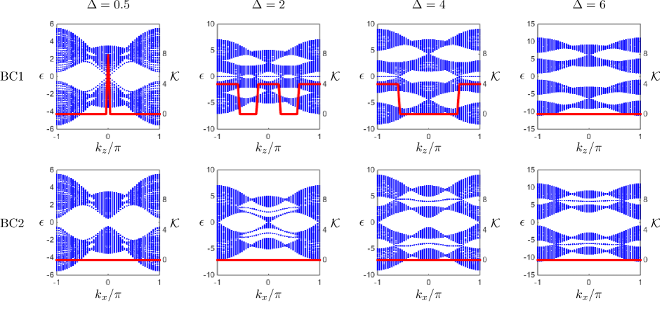
Figure 7: (Color online) Energy spectrum (blue scatter plot) and degeneracy indicator $\mathcal{K}_{k_{z}}(0)$ for the zero energy level (red solid line) in the large-$N$ limit for BC1 (top panel) vs. BC2 (bottom panel) for various values of the SC pairing $\Delta$. The other parameters are $\mu=0$, $t=\lambda=u_{cd}=1$, $N_{x}=120,$ $N_{y}=30$.

IV.4.1 Analysis of anomalous bulk-boundary correspondence
via boundary matrix

The relevant model Hamiltonian in real space is

$$\widehat{H}\!=\!\frac{1}{2}\sum_{{\mathbf{j}}}\Big{(}\hat{\Psi}^{\dagger}_{{\mathbf{j}}}h_{\bm{0}}\hat{\Psi}_{{\mathbf{j}}}-4\mu\Big{)}+\frac{1}{2}\sum_{{\mathbf{r}}=\hat{x},\hat{z}}\!\Big{(}\sum_{{\mathbf{j}}}\hat{\Psi}^{\dagger}_{{\mathbf{j}}}h_{{\mathbf{r}}}\hat{\Psi}_{{\mathbf{j}}+{\mathbf{r}}}+\,\text{H.c.}\Big{)},$$

with respect to a local basis of fermionic operators given by $\hat{\Psi}^{\dagger}_{\mathbf{j}}\equiv\begin{bmatrix}c^{\dagger}_{{\mathbf{j}},\uparrow}&c^{\dagger}_{{\mathbf{j}},\downarrow}&d^{\dagger}_{{\mathbf{j}},\uparrow}&d^{\dagger}_{{\mathbf{j}},\downarrow}&c_{{\mathbf{j}},\uparrow}&c_{{\mathbf{j}},\downarrow}&d_{{\mathbf{j}},\uparrow}&d_{{\mathbf{j}},\downarrow}\end{bmatrix}$. Here,

$$h_{\bm{0}} = -\mu\tau_{z}+u_{cd}\tau_{z}\nu_{z}-\Delta\tau_{x}\nu_{y}\sigma_{x},$$

$$h_{\hat{x}(\hat{z})} = -t\tau_{z}\nu_{z}+i\lambda\nu_{x}\sigma_{x(z)},$$

with Pauli matrices $\tau_{v},\nu_{v},\sigma_{v},\ v=x,y,z$ for the Nambu, orbital, and spin space, respectively. This Hamiltonian can be verified to obey time-reversal and particle-hole symmetry, as well as a chiral symmetry $U_{K}\equiv\tau_{x}\nu_{z}$. The topological response of the system was studied in Ref. [Deng14, ] using a $\mathds{Z}_{2}\times\mathds{Z}_{2}$ indicator $(Q_{k_{\parallel}=0},Q_{k_{\parallel}=\pi})$, where $Q_{k_{\parallel}}$ stands for the parity of the partial Berry phase sum for the value of transverse momentum Notenotation $k_{\parallel}$. The bulk-boundary correspondence of the system was studied subject to two different configurations: BC1, in which the system is periodic along $\hat{z}$ and open along $\hat{x}$, and BC2, in which the system is periodic along $\hat{x}$ and open along $\hat{z}$. A MFB emerges along the open edges for BC1 in the phase characterized by $(Q_{k_{z}=0},Q_{k_{z}=\pi})=(1,1)$. No MFB exists in the configuration BC2.

To shed light into this anomalous bulk-boundary correspondence using our generalized Bloch theorem framework, consider first the configuration BC1. Then, if $N_{x}$ denotes the size of the lattice along the $\hat{x}$ direction, $\widehat{H}$ decouples into $N_{x}$ virtual wires, parametrized by the transverse momentum $k_{z}$. These virtual $D=1$ Hamiltonians have the form

$$H_{k_{z},N_{x}} = \frac{1}{2}\sum_{j=1}^{N_{x}}\Big{(}\hat{\Psi}^{\dagger}_{j,k_{z}}h_{k_{z},0}\hat{\Psi}_{j,k_{z}}-4\mu\Big{)}$$

$$+ \frac{1}{2}\sum_{j=1}^{N_{x}-1}\!\Big{(}\hat{\Psi}^{\dagger}_{j,k_{z}}h_{k_{z},1}\hat{\Psi}_{j+1,k_{z}}+\text{H.c.}\Big{)},$$

where $h_{k_{z},0}\equiv h_{\bm{0}}+(e^{ik_{z}}h_{\hat{z}}+\text{H.c.})$ and $h_{k_{z},1}\equiv h_{\hat{x}}.$ The total number of Majorana modes hosted by each such chain (on its two ends) is given by the degeneracy indicator introduced in Part I [Sec. VI], namely, $\mathcal{K}(0)\equiv\text{dim}\ \text{ker}[{B}_{\infty}(0)],$ where ${B}_{\infty}(0)$ is the boundary matrix in the large-$N$ limit that we obtain after appropriately rescaling the extended bulk solutions corresponding to $|z_{\ell}|>1$, and removing the un-normalizable extended solutions corresponding to $|z_{\ell}|=1$. We calculate the above degeneracy indicator $\mathcal{K}(0)\equiv\mathcal{K}_{k_{z}}(0)$ for each wire parametrized by $k_{z}$, by evaluating the boundary matrix numerically. Representative results are shown in the top panel of Fig. 7. When the system is in a phase characterized by $(Q_{k_{z}=0},Q_{k_{z}=\pi})=(1,-1)$ ($\Delta=2$) and $(Q_{k_{z}=0},Q_{k_{z}=\pi})=(-1,-1)$ ($\Delta=4$) there are $\mathcal{O}(N)$ chains, each of them hosting four Majoranas (two pairs per edge). This is reflected in the four-fold degeneracy for a continuum of values of $k_{z}$. The values of $k_{z}$ at which the excitation gap closes are also the points at which the indicator changes its nature.

The same analysis may be repeated for BC2, in which case periodic BCs are imposed along $\hat{x}$ instead. The resulting virtual $D=1$ systems are now parametrized by $k_{x}$, with explicit expressions for the internal matrices given by $h_{k_{x},0}=h_{\bm{0}}+(e^{ik_{x}}h_{\hat{x}}+\text{H.c.})$ and $h_{k_{x},1}=h_{\hat{z}}.$ In the BC2 configuration, the degeneracy indicator remains zero, showcasing the absence of MFBs, see bottom panel of Fig. 7.

IV.4.2 Penetration depth of flat-band Majorana modes

Whether and how far the Majorana modes in the flat band penetrate in the bulk is important from the point of view of scattering. Our generalized Bloch theorem allows us to obtain a good estimate of the penetration depth without diagonalizing the system. In the large-$N$ limit, the wavefunction corresponding to a Majorana mode for a single wire described by $H_{k_{z},N_{x}}$ must include left emergent solutions and decaying extended solutions, so that

$$|\epsilon=0\rangle=\sum_{s=1}^{s_{0}}\alpha_{s}^{-}|\psi_{k_{z}s}^{-}\rangle+\sum_{|z_{\ell}|<1}\sum_{s=1}^{s_{\ell}}\alpha_{\ell s}|\psi_{k_{z}\ell s}\rangle,$$

for complex amplitudes $\{\alpha_{s}^{-},\alpha_{\ell s}\}$. The emergent solutions are perfectly localized, and so the penetration depth is determined by the extended solutions only. The latter are labeled by the roots $\{z_{\ell}\}$, computed at $\epsilon=0$, of the polynomial equation $z^{dR}\det(H_{k_{z}}(z)-\epsilon\mathds{1}_{8})=0$, which is the dispersion relation. Each extended solution $|\psi_{k_{z}\ell s}\rangle$ corresponding to the root $z_{\ell},\ |z_{\ell}|<1$ has penetration depth $(-\ln|z_{\ell}|)^{-1}$. A useful estimate of the penetration depth $\delta_{p}$ of a zero energy mode may then by obtained by taking the maximum of the individual penetration depths of the bulk solutions Lee81 , leading to the expression

$$\delta_{p}\equiv(-\ln|z_{p}|)^{-1},\quad|z_{p}|\equiv\max\,\{|z_{\ell}|,\ |z_{\ell}|<1\}.$$

Since the roots $\{z_{\ell}\}$ depend on the value of the transverse momentum $k_{z}$, so does the penetration depth $\delta_{p}$. As seen in Fig. 8, the Majoranas penetrate more inside the bulk near the critical values of the transverse momentum, where the excitation gap closes. At these points, the penetration depth diverges, signifying that the corresponding Majorana excitations become part of the bulk bands.

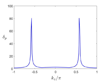
Figure 8: (Color online) Penetration depth (in units of the lattice constant) of flat-band Majoranas as a function of $k_{z}$. The parameters are $\mu=0$, $u_{cd}=t=\lambda=1$, $\Delta=4$.

IV.4.3 Impact of a Majorana flat band on Josephson current

Beside resulting in an enhanced local DOS at the surface Deng14 , one expects that the MFB may impact the nature of the equilibrium (DC) Josephson current at zero temperature. We now show (numerically) that the Josephson current flowing through a strip of finite width is $4\pi$-periodic, irrespective of the width of the strip. This is at variance with the behavior expected for a gapped $D=2$ $s$-wave TSC, in which case the $4\pi$-periodic contribution resulting from a fixed number of Majorana modes is washed away once the strip width becomes large.

We model a SNS junction of the SC under investigation by letting the normal part be a weak link with the same type of hopping, spin-orbit coupling and hybridization as the SC, but weaker by a factor of $w=0.2$. The DC Josephson current can be calculated using the formula lesovik11

$$I(\phi)=\frac{2e}{\hbar}\frac{\partial E_{0}}{\partial\phi}=-\frac{2e}{\hbar}\sum_{\epsilon_{n}>0}\frac{\partial\epsilon_{n}}{\partial\phi},$$

where $E_{0}$ is the energy of the many-body ground state, $\epsilon_{n}$ are single-particle energy levels, and $\phi$ is the SC phase difference (or flux). As $\phi$ is varied, at the level crossings of low-lying energy levels with the many-body ground state associated with the $4\pi$-periodic effect, the system continues in the state which respects fermionic parity and time-reversal symmetry in all the virtual wires.

The upper panels of Fig. 9 show the Josephson response $I(\phi)$ of the gapless TSC under the two BCs. While in the BC1 configuration the behavior of the current $I(\phi)$ (solid black line) is $4\pi$-periodic, the BC2 configuration displays standard $2\pi$-periodicity, reflecting the presence of the MFB only under BC1. The lower panels of Fig. 9 show the Josephson response of the gapped $s$-wave TSC model introduced and analyzed in Ref. [swavePRL, ; swavePRB, ]. It can be seen that the Josephson current is now identical under BC1 and BC2, as expected from the fact that a standard bulk-boundary correspondence is in place.

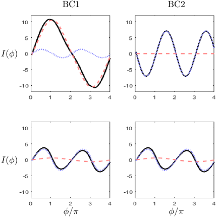
Figure 9: (Color online) Total Josephson current $I(\phi)$ (black solid line), $2\pi$-periodic component $I_{2\pi}(\phi)$ (blue dotted line) and $4\pi$-periodic component $I_{4\pi}(\phi)$ (red dashed line) in units of $2e/\hbar$, as a function of flux $\phi$. Top (bottom) panels correspond to the gapless (gapped) model of a $D=2$ $s$-wave TSC, whereas left (right) panels correspond to BC1 (BC2), respectively. The parameters used for both models are $\mu=0$, $u_{cd}=t=\lambda=1$, $\Delta=4$, $N_{x}=N_{z}=60$.

Let us separate the total Josephson current $I(\phi)$ into $2\pi$- and $4\pi$-periodic components by letting $I(\phi)=I_{2\pi}(\phi)+I_{4\pi}(\phi)$, with

$$I_{2\pi}(\phi)\equiv\left\{\begin{array}[]{lcl}\frac{1}{2}[I(\phi)+I(\phi+2\pi)]&\text{if}&0\leq\phi<2\pi\\[2.0pt] \frac{1}{2}[I(\phi)+I(\phi-2\pi)]&\text{if}&2\pi\leq\phi<4\pi\end{array}\right.,$$

$$I_{4\pi}(\phi)\equiv\left\{\begin{array}[]{lcl}\frac{1}{2}[I(\phi)-I(\phi+2\pi)]&\text{if}&0\leq\phi<2\pi\\[2.0pt] \frac{1}{2}[I(\phi)-I(\phi-2\pi)]&\text{if}&2\pi\leq\phi<4\pi\end{array}\right.,$$

In the four panels of Fig. 9, the $2\pi$- and $4\pi$-periodic components are individually shown by (blue) dotted and (red) dashed lines, respectively. The nature of the supercurrent in the gapped TSC (lower panels) is predominantly $2\pi$-periodic, with only a small $4\pi$-periodic component due to the presence of a finite number of Majoranas (two per edge). Further numerical simulations (data not shown) reveal that the amplitude of the $2\pi$-periodic current relative to the $4\pi$-periodic current increases linearly with the width of the strip, so that for large strip width, the Josephson current is essentially $2\pi$-periodic. The origin of such a degradation of the $4\pi$-periodicity lies in the fact that the number of Majorana modes is constant, irrespective of the width of the strip, as only one virtual wire hosts Majorana modes in this gapped model. Since only the Majorana modes can support $4\pi$-periodic current, their contribution relative to the extensive $2\pi$-periodic current arising from the bulk states diminishes as the strip width becomes large. In contrast, for the gapless TSC in the MFB phase (top panels), the number of virtual wires hosting Majorana modes grows linearly with the width of the strip in the BC1 configuration. This leads to an extensive contribution from the $4\pi$-periodic component, which may be easier to detect in experiments.

V Summary and Outlook

As mentioned in the Introduction, this paper constitutes the sequel, Part II, to Ref. [PRB1, ], where we introduced a generalization of Bloch’s theorem for arbitrary boundary conditions. In clean systems translation symmetry is only broken by surface terminations and boundary constraints that encode physical or experimental conditions. The conventional Bloch theorem is not in force because translational symmetry is explicitly broken. However, since such a symmetry is only mildly broken, one wonders whether one can one continue to label single-particle electronic excitations in terms of some kind of “generalized momenta”. Our generalized Bloch theorem PRL ; PRB1 provides a precise answer to that question. The mathematical framework makes the idea of approximate translation precise by relating the spectral properties of certain shift operators to non-unitary representations of the group of translations JPA . According to the generalized Bloch theorem, the exact eigenstates of a clean system of independent fermions with terminations are linear combinations of eigenstates of non-unitarily represented translations. It is because of this lack of unitarity that complex momenta arise. The latter leads to the emergence of localized edge modes and more involved power-law corrections to the Bloch-like wavefunctions. The amplitudes that weigh the relative contribution of the generalized Bloch states to the exact energy eigenstates are determined by a boundary matrix. This piece of our formalism, the boundary matrix, optimally combines information about the translation-invariant bulk and the boundary conditions: it allows one to compactly parametrize the manifold of boundary conditions and may eventually suggest new ways of accessing effective edge theories.

Part II focused on presenting two new theoretical developments and several non-trivial applications to higher-dimensional systems. New developments include the extension of the generalized Bloch theorem formalism to incorporate: (1) Surface reconstruction and surface disorder; and (2) Interface physics involving multiple bulks. Within our framework, boundary conditions for $D$-dimensional systems must be imposed on two parallel hyperplanes, but are otherwise arbitrary. Thus, the generalized Bloch theorem yields highly-effective tools for diagonalizing systems subject to anything from pristine terminations to surface relaxation, reconstruction and disorder. The extension to interfaces between multiple bulks allows us to study arbitrary junctions, including interface modes resulting from putting in contact two exotic topologically non-trivial bulks.

It is interesting to digress on what happens when one tries to formulate a generalized Bloch theorem for clean systems cut into hypercubes. The bulk-boundary separation goes through essentially unchanged: for example, the range of the boundary projector consists of a hypercubic surface layer of thickness determined by the bulk structure of the system. The challenge in higher dimensions is solving the bulk equation explicitly and in full generality. It is a worthy challenge, because it would yield insight into the plethora of corner states that can appear in such systems benalcazar17 ; hashimoto17 ; flore18 . While special cases may still be able to be handled on a case-by-case basis, in general we see little hope of using the same mathematical techniques (crucially, the Smith decomposition JPA ) that work so well in our setup. In general, the analytic continuation of the Bloch Hamiltonian become then a matrix-valued analytic function of $D$ complex variables. The passage from one complex variable to several makes a critical difference.

We have illustrated our formalism with several applications to models of current interest in condensed matter physics. Table 1 summarizes all systems that we have solved so far by our techniques, where exact analytic solutions were unknown prior to our findings, to the best of our knowledge. For example, we showed that it is possible to analytically determine Andreev bound states for an idealized SNS junction. More importantly, the existence of power-law modes would not have been unveiled without our mathematical formalism. Among the challenging applications presented in this paper, we investigated in detail the Creutz ladder system, where thanks to a Gaussian duality equivalence , we can map this topological insulator to a pair of coupled Kitaev Majorana chains. The presence of power-law topological modes in the Creutz ladder insulator is noteworthy, see Sec. IV.1. We also find power-law modes on the surface of the $p+ip$ chiral superconductor as part of our closed-form full calculation of the surface states of this system, see Sec. IV.3. It seems reasonable now to accept that power-law modes, topological or otherwise, are a general, if fine-tuned, feature of short range tight-binding models. We have also included applications to other $D=2$ systems, such as the full closed-form diagonalization of graphene ribbons for zigzag-bearded and armchair surface terminations. While the edge modes for zigzag-bearded graphene have been computed before in closed form, the closed-form band states appear to be new in the literature. It seems a distinctive feature of the generalized Bloch theorem that both edge and bulk bands can be treated analytically on equal footing. Finally, we investigated in detail the Majorana flat bands of the gapless $s$-wave topological superconductor we previously introduced Deng14 . There, we find an extensive contribution of the surface Majorana flat band to the $4\pi$-periodic component of the Josephson current, which would serve as a smoking gun for experimental detection should a candidate material realization be identified.

In view of these results it seems fair to grant that the generalized Bloch theorem bestows a higher level of control over surface and interface physics, and opens the door for a deeper investigation of the interplay between surface/interface and bulk critical phenomena book8 ; quelle15 ; kempkes16 . Let us conclude by recalling a main motivation behind the formulation of our generalized Bloch theorem. That motivation was to investigate the bulk-boundary correspondence in boundary space, that is, the space of boundary conditions, as opposed to the usual parameter space, in order to quantitatively express stability and robustness in this new space that clearly affects boundary invariants most directly prodanBook . Physically, boundary conditions are idealized representations of interfaces between the system of interest and an “environment” that we choose not to characterize, and so they capture matching conditions that can have a big impact on the energy spectrum of the system. This interpretation suggests that it might be very illuminating to bring closer together precise mathematical ideas of stability and robustness from quantum information processing and control engineering, and more qualitative concepts in condensed matter physics. We have not carried out this systematic task in this paper which is, strictly speaking, still an exploration of the power of the generalized Bloch theorem. We will return to the study of the relation between boundary and bulk topological invariants in future publications.

Appendix A A criterion for the absence of localized eigenstates

Symmetry conditions paired with suitable BCs can exclude completely edge modes, topological or otherwise. We have identified one particularly useful sufficient condition that guarantees the absence of edge modes. It relies on the analytic diagonalization of the matrices

$$T_{\theta}+T_{\theta}^{\dagger}\equiv e^{-i\theta}T+e^{i\theta}T^{\dagger},\quad\theta\in[0,2\pi).$$

Physically, the phase $\theta$ may arise from ${\mathbf{k}}_{\parallel}$, see for example Sec. IV.2.2, or one may think of $\theta$ as an applied electric field. The combination $T+T^{\dagger}$ is singled out by a symmetry argument. The $\mathds{Z}_{2}$ mirror symmetry,

$$U_{\sf m}\equiv\sum_{j=1}^{N}|N-j+1\rangle\langle j|,\quad U_{\sf m}^{\dagger}=U_{\sf m}^{-1}=U_{\sf m},$$

exchanges the two shift operators, $U_{\sf m}TU_{\sf m}=T^{\dagger}$, so that

$$U_{\sf m}(T+T^{\dagger})U_{\sf m}=T^{\dagger}+T.$$

The eigenstates and eigenvalues of $T+T^{\dagger}$ are known MouraSin , and were recomputed by way of the generalized Bloch theorem in Part I (see Sec. V A therein):

$$(T+T^{\dagger})|k_{q}\rangle=2\cos\big{(}\frac{\pi q}{N+1}\big{)}|k_{q}\rangle,\quad q=1,\dots,N,$$

with unnormalized eigenvectors

$$|k_{q}\rangle=\sum_{j=1}^{N}\sin\big{(}\frac{\pi qj}{N+1}\big{)}|j\rangle.$$

Let $X\equiv\sum_{j=1}^{N}j\,|j\rangle\langle j|$ denote the position operator. As explained in Part I (see Appendix B), $[X,T]=-T$, and thus $e^{i\theta X}Te^{-i\theta X}=e^{-i\theta}T$. In particular,

$$e^{i\theta X}(T+T^{\dagger})e^{-i\theta X}=e^{-i\theta}T+e^{i\theta}T^{\dagger}.$$

It follows that the eigenstates of $T_{\theta}+T_{\theta}^{\dagger}$ are given by

$$|k_{q},\theta\rangle=\sum_{j=1}^{N}\sin\big{(}\frac{\pi qj}{N+1}\big{)}e^{i\theta j}|j\rangle,\quad q=1,\dots,N.$$

Assume now that all the matrices ${h}_{r}$ entering the single-particle Hamiltonian of interest satisfy the relation

$$h_{r}^{\dagger}=e^{i2r\theta}h_{r},$$

for some choice of $\theta$, that is,

$$H=\mathds{1}_{N}\otimes h_{0}+\sum_{r=1}^{R}(T_{\theta}^{r}+T_{\theta}^{\dagger\,r})\otimes e^{ir\theta}h_{r}+W.$$

Then, it is easy to see that $H$ rewrites as

$$H=\mathds{1}_{N}\otimes h_{0}+\sum_{r=1}^{R}(T_{\theta}+T_{\theta}^{\dagger})^{r}\otimes\tilde{h}_{r}+W^{\prime}+W,$$

in terms of new hopping matrices $\tilde{h}_{r}$ and boundary contribution $W^{\prime}$ with the same range finite $R$ (for example, $(T+T^{\dagger})^{3}=T^{3}+3T-|1\rangle\langle 2|-|N-1\rangle\langle N|+{\rm H.c}.$). If the original BCs are such that $W=-W^{\prime}$, then $H$ can be expressed as a function of $T_{\theta}+T_{\theta}^{\dagger}$. It follows that no localized eigenstate can exist. This is exactly the situation for armchair graphene, see Sec. IV.2.2.

Appendix B The BCS chain

A tight-binding BCS chain with $N$ lattice sites can be modeled in terms of the Hamiltonian bena12

$$\widehat{H} = -\sum_{j,\sigma}(tc^{\dagger}_{j\sigma}c_{j+1\sigma}+\frac{\mu}{2}c^{\dagger}_{j\sigma}c_{j\sigma}+\text{H.c.})$$

$$- \sum_{j}(\Delta c_{j\uparrow}^{\dagger}c_{j\downarrow}^{\dagger}+\text{H.c.}).$$

The single-particle Hamiltonian associated to $\widehat{H}_{\sf S}$ is

$$H_{N}=\mathds{1}_{N}\otimes h_{0}+(T+T^{\dagger})\otimes h_{1},$$

where we assume open BCs, with

$$h_{0}=-\mu\tau_{z}\otimes\mathds{1}_{2}-\Delta\tau_{y}\otimes\sigma_{y},\quad h_{1}=-t\tau_{z}\otimes\mathds{1}_{2}.$$

$H_{N}$ commutes with $\mathcal{S}=\mathds{1}_{N}\otimes\mathds{1}_{2}\otimes\sigma_{y}$ because total spin is conserved. Thus, following the discussion in Sec. II.3, we can block-diagonalize $H_{N}$ as

$$H_{N}=\sum_{{\rm s}=\pm 1}H_{N,{\rm s}}\otimes|{\rm s}\rangle\langle{\rm s}|,$$

where $|{\rm s}\rangle$ denotes the eigenstate of $\sigma_{y}$ for the eigenvalue ${\rm s}=\pm 1$. The internal matrices for $H_{N,{\rm s}}$ are

$$h_{{\rm s},0}=-\mu\tau_{z}-{\rm s}\,\Delta\tau_{y},\quad h_{{\rm s},1}=-t\tau_{z},$$

and the action of the particle-hole symmetry on the blocks is

$$\mathcal{P}H_{N,{\rm s}}\otimes|{\rm s}\rangle\langle{\rm s}|\mathcal{P}^{-1}=$$ (40)

$$=\tau_{x}H_{N,s}^{*}\tau_{x}\otimes(|{\rm s}\rangle\langle{\rm s}|)^{*}=-H_{N,-{\rm s}}|-{\rm s}\rangle\langle-{\rm s}|.$$

Hence, the two blocks are exchanged by particle-hole symmetry, whereas the full Hamiltonian only changes sign. Note that, taken individually, these blocks do not respect the particle-hole symmetry because of Eq. (40). Therefore, the many-body Hamiltonian does not decouple into two blocks.

The nontrivial spatial structure of each of the two blocks is encoded in the matrix $T+T^{\dagger}$. According to Appendix A, this fact suffices to guarantee the absence of edge modes and goes a long way towards analytic solvability. For open BCs the eigenstates are

$$|\epsilon_{n,q},{\rm s}\rangle=\sum_{j=1}^{N}\sin(\frac{\pi qj}{N+1})|j\rangle\begin{bmatrix}i\rm{s}\Delta\\ \epsilon_{n,q}+\mu+2t\cos(\frac{\pi q}{N+1})\end{bmatrix},$$

with $q=1,2,\dots,N$ and $n=1,2$ the band index for spin $\rm{s}$ along the $y$ direction. The energy $\epsilon_{n,q}$ satisfies the relation

$$\epsilon_{n,q}=(-1)^{n}\sqrt{\Big{(}\mu+2t\cos(\frac{\pi q}{N+1})\Big{)}^{2}+|\Delta|^{2}}.$$ (41)

Appendix C An SNS junction

With reference to Sec. III, our aim is to find the exact Andreev bound states that form on the normal region. The block-diagonalization in spin space reduces to solving the boundary value problem for the blocks with reduced internal space. Because of Eq. (40), note that each spin block does not individually describe an SNS junction Hamiltonian. The SNS junction is modeled as the system formed by attaching a finite metallic N chain to two semi-infinite SC chains, S1 and S2, with the length of the metallic chain being $N=4{\sf L}-1$ for some positive integer ${\sf L}$. The projectors corresponding to the left and right semi-infinite S1 and S2 regions are

$$P_{1}=\sum_{j=-\infty}^{-2{\sf L}}|j\rangle\langle j|,\quad P_{2}=\sum_{j=2{\sf L}}^{\infty}|j\rangle\langle j|,$$

whereas the region N is finite with an associated projector

$$P_{3}=\sum_{j=-2{\sf L}+1}^{2{\sf L}-1}|j\rangle\langle j|.$$

The links connecting the SC regions S1, S2 to the metal region N at $j=-2{\sf L}$ and $j=2{\sf L}-1$ have weaker hopping strength $t^{\prime}$, and we set the chemical potential $\mu\equiv 0$. The metallic chain is therefore modeled by only the NN hopping of strength $t$, and links to the two SC leads by way of a hopping amplitude $t^{\prime}<t$. The Hamiltonian of the full system is $\widehat{H}_{\sf SNS}=\widehat{H}_{\sf S1}+\widehat{H}_{\sf S2}+\widehat{H}_{\sf T}+\widehat{H}_{\sf N},$ with the SC and tunneling Hamiltonians given in Eqs. (20)-(21) in the main text. Note that the relevant matrices $h_{0},h_{1}$ for the metal part can be obtained from the ones for the SC part (in Appendix B) by setting $\Delta=0$.

The single-particle Hamiltonian $H_{\sf SNS}$ of the junction is block-diagonalized in the basis of the spin operator $\sigma_{y}$, and the two blocks are related to each other by the particle-hole symmetry in the same way as described by Eq. (40). Let us focus on the ${\rm s}=+1$ block, and denote it by $H_{+}$. This system has three translation-invariant regions (bulks) connected by two internal boundaries. The energy eigenvector ansatz in this case is obtained by extending the ansatz in Eq. (19) in the main text to a system of three bulks.

Consider first the case with no phase difference between the two SC leads S1 and S2, that is, $\Delta_{1}=\Delta_{2}=\Delta$ for a real value of $\Delta$. Note that $H_{+}$ obeys a mirror symmetry about $j=0$,

$$\mathcal{S}_{1}=\sum_{j\in\mathds{Z}}|-j\rangle\langle j|\otimes\mathds{1}_{2},$$

and another local symmetry,

$$\mathcal{S}_{2}=\sum_{j\in\mathds{Z}}(-1)^{j}|j\rangle\langle j|\otimes\tau_{y}.$$

Since we are only interested in the states bound on the metal N region, we restrict the value of energy to be in the band gap of the SCs, which is $(-\Delta,\Delta)$. For these bound states to carry a superconducting current, they must be of extended nature on the metallic region, which is allowed by energies such that $|\epsilon|<|t|$.The eigenstate ansatz for any such energy in each of the three bulks will be in terms of the roots of Eq. (41), with $\mu=0$. Noting appropriate symmetries of the polynomial, we denote the four roots in the bulks of S1 and S2 by $\{z_{1},z^{-1}_{1},-z_{1},-z^{-1}_{1}\}$. Without loss of generality, we can choose $|z_{1}|>1$ and $t(z_{1}+z^{-1}_{1})=i{\sf D}$, with ${\sf D}\equiv\sqrt{\Delta^{2}-\epsilon^{2}}$. From Eq. (41) and the above constraints, we find that

$$z_{1}=-\frac{{\sf D}+\sqrt{{\sf D}^{2}+4t^{2}}}{2it}.$$ (42)

For an exponentially decaying mode in the S1 and S2 region, the ansatz is given by

$$P_{1}|\epsilon,{\rm s}_{1},{\rm s}_{2},\bm{\alpha}\rangle=\alpha_{1}\Big{(}P_{1}|z_{1},1\rangle\begin{bmatrix}i\Delta\\ \epsilon+i{\sf D}\end{bmatrix}\\ +{\rm s}_{2}P_{1}|-z_{1},1\rangle\begin{bmatrix}{\sf D}-i\epsilon\\ -\Delta\end{bmatrix}\Big{)},$$

$$P_{2}|\epsilon,{\rm s}_{1},{\rm s}_{2},\bm{\alpha}\rangle=\alpha_{1}\Big{(}{\rm s}_{1}P_{2}|\frac{1}{z_{1}},1\rangle\begin{bmatrix}i\Delta\\ \epsilon+i{\sf D}\end{bmatrix}\\ +{\rm s}_{1}{\rm s}_{2}P_{2}|-\frac{1}{z_{1}},1\rangle\begin{bmatrix}{\sf D}-i\epsilon\\ -\Delta\end{bmatrix}\Big{)},$$

respectively, where ${\rm s}_{1},{\rm s}_{2}$ denote eigenvalues of symmetries $\mathcal{S}_{1}$ and $\mathcal{S}_{2}$ respectively. For the metallic region, since $\Delta=0$, all four roots lie on the unit circle. We denote them by $\{w_{1},w^{-1}_{1},-w_{1},-w^{-1}_{1}\}$, with the convention $t(w_{1}+w_{1}^{-1})=-\epsilon$. Then the ansatz for the N region can be written as

$$P_{3}|\epsilon,{\rm s}_{1},{\rm s}_{2},\bm{\alpha}\rangle=\alpha_{2}\big{(}P_{3}|w_{1},1\rangle+{\rm s}_{1}P_{3}|1/w_{1},1\rangle\begin{bmatrix}1\\ 0\end{bmatrix}+\\ {\rm s}_{2}P_{3}|-w_{1},1\rangle+{\rm s}_{1}{\rm s}_{2}P_{3}|-1/w_{1},1\rangle\big{)}\begin{bmatrix}0\\ i\end{bmatrix}.$$

Therefore, we have obtained four eigenstate ansätze corresponding to the four cases $\{{\rm s}_{1}=\pm 1,\ {\rm s}_{2}=\pm 1\}$, which we denote by $|\epsilon,{\rm s}_{1},{\rm s}_{2},\bm{\alpha}\rangle$, where $\bm{\alpha}=[\alpha_{1}\;\alpha_{2}]^{\rm T}$ are the free parameters. The BCs are provided by the weak links, that is, $j=\pm 2{\sf L},\pm(2{\sf L}-1)$. We choose the basis $\{|2{\sf L},{\rm s}_{1},{\rm s}_{2}\rangle,\ |2{\sf L}-1,{\rm s}_{1},{\rm s}_{2}\rangle,\ {\rm s}_{1},{\rm s}_{2}=1,-1\}$ of the boundary subspace, where

$$|2{\sf L},{\rm s}_{1},{\rm s}_{2}\rangle\! \equiv \frac{1}{2}(|-2{\sf L}\rangle+{\rm s}_{1}|2{\sf L}\rangle)\begin{bmatrix}1\\ i{\rm s}_{2}\end{bmatrix},$$

$$|2{\sf L}-1,{\rm s}_{1},{\rm s}_{2}\rangle\! \equiv \frac{1}{2}(|-2{\sf L}+1\rangle+{\rm s}_{1}|2{\sf L}-1\rangle)\begin{bmatrix}1\\ -i{\rm s}_{2}\end{bmatrix}\!.$$

There will be four boundary matrices $B(\epsilon,{\rm s}_{1},{\rm s}_{2})$, for ${\rm s}_{1},{\rm s}_{2}=1,-1$, arising from the equations

$$\langle 2{\sf L},{\rm s}_{1},{\rm s}_{2}|(H-\epsilon\mathds{1}_{2}))|\epsilon,{\rm s}_{1},{\rm s}_{2},\bm{\alpha}\rangle=0,$$

$$\langle 2{\sf L}-1,{\rm s}_{1},{\rm s}_{2}|(H-\epsilon\mathds{1}_{2}))|\epsilon,{\rm s}_{1},{\rm s}_{2},\bm{\alpha}\rangle=0.$$

The boundary matrix corresponding to $({\rm s}_{1},{\rm s}_{2})$ is

$$B(\epsilon,{\rm s}_{1},{\rm s}_{2})=\\ \begin{bmatrix}tz_{1}^{-2{\sf L}+1}(i\Delta-{\rm s}_{2}({\sf D}-i\epsilon))&-t^{\prime}(w_{1}^{-2{\sf L}+1}+s_{1}w_{1}^{2{\sf L}-1})\\ -t^{\prime}z_{1}^{-2{\sf L}}(i\Delta+{\rm s}_{2}({\sf D}-i\epsilon))&t(w_{1}^{-2{\sf L}}+s_{1}w_{1}^{2{\sf L}})\end{bmatrix}.$$

In writing the above, we made use of the identity

$$(h_{0}-\epsilon\mathds{1}+z_{\ell}h_{1})|u_{\ell}\rangle=-z_{\ell}^{-1}h_{1}^{\dagger}|u_{\ell}\rangle,$$

which follows from the bulk equation. The condition for non-trivial kernel of the boundary matrix in the four cases leads, after simplification using Eq. (42), to the following four boundary equations:

$$-\left(\frac{t^{\prime}}{t}\right)^{2}\!\!\left(\frac{2t}{\epsilon+{\rm s}_{2}\Delta}\right)\left(1+\sqrt{1+\frac{4t^{2}}{\Delta^{2}-\epsilon^{2}}}\right)^{-1}=$$

$$\frac{\cos k(2{\sf L}-1)}{\cos k(2{\sf L})},\quad\text{if}\quad{\rm s}_{1}=+1,{\rm s}_{2}=\pm 1\qquad$$ (43a)

$$-\left(\frac{t^{\prime}}{t}\right)^{2}\!\!\left(\frac{2t}{\epsilon+{\rm s}_{2}\Delta}\right)\left(1+\sqrt{1+\frac{4t^{2}}{\Delta^{2}-\epsilon^{2}}}\right)^{-1}=$$

$$\frac{\sin k(2{\sf L}-1)}{\sin k(2{\sf L})},\quad\text{if}\quad{\rm s}_{1}=-1,{\rm s}_{2}=\pm 1,\qquad$$ (43b)

where $e^{ik}\equiv w_{1}$. Whenever any one of these conditions is satisfied, $\epsilon$ is an eigenvalue. The coefficients $\alpha_{1},\alpha_{2}$, that completely determine the eigenstates in the four cases, in turn satisfy

$$\frac{\alpha_{2}}{\alpha_{1}}=\Big{(}\frac{t^{\prime}}{t}\,\Big{)}\frac{z_{1}^{-2{\sf L}}(i\Delta+{\rm s}_{2}({\sf D}-i\epsilon))}{2\cos k(2{\sf L})},\;\;\text{if}\;{\rm s}_{1}=+1,{\rm s}_{2}=\pm 1,$$

$$\frac{\alpha_{2}}{\alpha_{1}}=\Big{(}\frac{t^{\prime}}{t}\,\Big{)}\frac{z_{1}^{-2{\sf L}}(i\Delta+{\rm s}_{2}({\sf D}-i\epsilon))}{2\sin k(2{\sf L})},\;\;\text{if}\;{\rm s}_{1}=-1,{\rm s}_{2}=\pm 1.$$

The structure of the above boundary equations explains how the number of bound modes increases as we increase $N$ or $\Delta$. Notice that the function on the right hand side of Eq. (43) assume all real values between any two adjacent poles, given by

$$k=\frac{\pi q}{2{\sf L}-1}+\frac{\pi}{2(2{\sf L}-1)},\quad q=0,1,\dots,2{\sf L}-2.$$

When the metal strip is completely disconnected from the SC, that is, when $t^{\prime}=0$, the bound states corresponding to ${\rm s}_{1}=+1$ in the metal are given by

$$k=\frac{\pi q}{2{\sf L}}+\frac{\pi}{4{\sf L}},\quad q=0,1,\dots,2{\sf L}-1,$$

each of which lie singularly between two adjacent poles. This can be seen from the relation

$$\frac{\pi q}{2{\sf L}-1}>\frac{\pi q}{2{\sf L}}>\frac{\pi(q-1)}{2{\sf L}-1}.$$

This analysis indicates that each metallic state at energy less than $\Delta$ gets converted into a bound state with slightly different value of energy in the presence of weak tunneling. For a fixed value of $\Delta$, increasing $N$ implies more poles for the functions on the right hand-side, therefore allowing more solutions of the boundary equations, as discussed in the main text.

Appendix D The Creutz ladder

In terms of the array $\hat{\Psi}_{j}^{\dagger}=\begin{bmatrix}a_{j}^{\dagger}&b_{j}^{\dagger}\end{bmatrix},$ the single-particle Hamiltonian for the Creutz ladder, given by Eq. (IV.1) in the main text, is specified by the matrices

$${h}_{0}=-\begin{bmatrix}0&{\sf M}\\ {\sf M}&0\end{bmatrix},\quad{h}_{1}=-\begin{bmatrix}{\sf K}e^{i\theta}&{\sf K}{\sf r}\\ {\sf K}{\sf r}&{\sf K}e^{-i\theta}\end{bmatrix}.$$

It is more convenient, however, to work with the equivalent ladder Hamiltonian $\widetilde{H}_{N}=\mathds{1}_{N}\otimes\tilde{h}_{0}+(T\otimes\tilde{h}_{1}+\text{H.c.})$ defined in Eq. (24), where the new matrices

$$\tilde{h}_{0}=\!-\!\begin{bmatrix}{\sf M}\!&0\\ 0\!&-{\sf M}\end{bmatrix}\!,\tilde{h}_{1}=-\begin{bmatrix}{\sf K}({\sf r}+\cos\theta)&{\sf K}\sin\theta\\ -{\sf K}\sin\theta&{\sf K}(-{\sf r}+\cos\theta)\end{bmatrix}.$$

The analytic continuation of the corresponding Bloch Hamiltonian is

$$\widetilde{H}(z)=-\begin{bmatrix}{\sf M}+{\sf K}({\sf r}+\cos\theta)(z+z^{-1})&{\sf K}\sin\theta\,(z-z^{-1})\\ -{\sf K}\sin\theta\,(z-z^{-1})&-{\sf M}+{\sf K}(-{\sf r}+\cos\theta)(z+z^{-1})\end{bmatrix},$$

and the condition $\det(\widetilde{H}(z)-\epsilon\mathds{1}_{2})=0$ yields the polynomial equation

$$P(\epsilon,z)=-z^{2}\big{[}({\sf r}^{2}-1){\sf K}^{2}(z+z^{-1})^{2}+2{\sf K}({\sf M}{\sf r}-\epsilon\cos\theta)(z+z^{-1})+{\sf M}^{2}+4{\sf K}^{2}\sin^{2}\theta-\epsilon^{2}\big{]}=0.$$ (44)

For fixed but arbitrary values of the parameters, the singular, that is, flat-band energies, can be determined as the solutions in $\epsilon$ of the system of equations

$$({\sf r}^{2}-1){\sf K}^{2}=0,$$

$${\sf K}({\sf M}{\sf r}-\epsilon\cos\theta)=0,$$

$${\sf M}^{2}+4{\sf K}^{2}\sin^{2}\theta-\epsilon^{2}=0,$$

For any combination of parameter values that exclude flat bands, the generalized Bloch theorem can be used to determine all the (regular) energy eigenvalues and eigenstates. For this system, there are $2Rd=4$ independent solutions of the bulk equation for each value of $\epsilon$, and they are all extended. Excluding power-law modes, these extended bulk solutions are labeled by the distinct roots of Eq. (44). The solution $|u(\epsilon,z_{\ell})\rangle$ of the kernel equation $(\widetilde{H}(z_{\ell})-\epsilon\mathds{1}_{2})|u\rangle=0$ can be taken to be

$$|u(\epsilon,z_{\ell})\rangle=\begin{bmatrix}a(z_{\ell})\\ \epsilon+b(z_{\ell})\end{bmatrix},$$ (45)

$$a(z)=-{\sf K}\sin\theta\,(z-z^{-1}),$$

$$b(z)={\sf M}+{\sf K}({\sf r}+\cos\theta)\,(z+z^{-1}).$$

For ${\sf r}\neq\pm 1$, $h_{1}$ is invertible, and we get total four roots which come in reciprocal pairs. We choose the convention $z_{1}=z_{3}^{-1}$, $z_{2}=z_{4}^{-1},\quad|z_{1}|,|z_{2}|\leq 1$ to denote them. Then the ansatz is

$$|\epsilon,\bm{\alpha},\bm{\beta}\rangle=\sum_{\ell=1,2}\Big{(}\alpha_{\ell}|z_{\ell},1\rangle|u(\epsilon,z_{\ell})\rangle+\beta_{\ell}|z_{\ell}^{-1},1\rangle|u(\epsilon,z_{\ell}^{-1})\rangle\Big{)},$$

with amplitudes $(\bm{\alpha},\bm{\beta})=(\{\alpha_{\ell}\},\{\beta_{\ell}\})$ to be determined by the boundary matrix.

It is useful at this point to cast the ansatz in a more symmetric form. The unitary operator

$$\mathcal{S}=-\sum_{j=1}^{N}|N+1-j\rangle\langle j|\otimes\begin{bmatrix}1&0\\ 0&-1\end{bmatrix},$$ (46)

describes a $\mathds{Z}_{2}$ symmetry of the Hamiltonian in Eq. (IV.1). It commutes with the bulk projector $P_{B}$, so that

$$[\mathcal{S},P_{B}(H_{N}-\epsilon)]=0.$$

Following Sec. II.3, this allows us to partition the bulk solution space into ${\rm s}=+1$ and ${\rm s}=-1$ eigenspaces of $\mathcal{S}$. Notice that under this transformation,

$$\mathcal{S}|z_{\ell},1\rangle|u(\epsilon,z_{\ell})\rangle=\sum_{j=1}^{N}|N+1-j\rangle\langle j|z_{\ell},1\rangle\otimes\begin{bmatrix}-a(z_{\ell})\\ \epsilon+b(z_{\ell})\end{bmatrix}\\ =z_{\ell}^{N+1}|z_{\ell}^{-1},1\rangle\begin{bmatrix}a(z_{\ell}^{-1})\\ \epsilon+b(z_{\ell}^{-1})\end{bmatrix}=z_{\ell}^{N+1}|z_{\ell}^{-1},1\rangle|u(\epsilon,z_{\ell}^{-1})\rangle.$$

This equation is a consequence of the symmetry

$$\sigma_{z}\widetilde{H}(z)\sigma_{z}=\widetilde{H}(z^{-1}),\quad\sigma_{z}=\begin{bmatrix}1&0\\ 0&-1\end{bmatrix}$$

of the reduced bulk Hamiltonian. Therefore, the ansatz yields eigenstates of $\mathcal{S}$ provided $z_{\ell}^{N+1}\alpha_{\ell}=\pm\beta_{\ell}$. For each energy, we obtain two ansätze,

$$|\epsilon,{\rm s},\bm{\alpha}\rangle=$$ (47)

$$\sum_{\ell=1,2}\alpha_{\ell}\{|z_{\ell},1\rangle|u(\epsilon,z_{\ell})\rangle+{\rm s}z_{\ell}^{N+1}|z_{\ell}^{-1},1\rangle|u(\epsilon,z_{\ell}^{-1})\rangle\},$$

corresponding to the eigenvalues ${\rm s}=\pm 1$. Each of these ansätze, with only two free parameters, is representative of the $D=2$ bulk solution space compatible with the corresponding eigenvalue of the symmetry.

The next step is to construct the boundary matrices corresponding to ${\rm s}=\pm 1$. We need to find a basis of the boundary subspace in which ${\rm s}$ is block-diagonal. One such basis is $\{|{\rm s},m\rangle,\,{\rm s}=1,-1,m=1,2\}$, where

$$|{\rm s},1\rangle\equiv\frac{1}{\sqrt{2}}(|1\rangle-{\rm s}|N\rangle)\begin{bmatrix}1\\ 0\end{bmatrix},\;\;|{\rm s},2\rangle\equiv\frac{1}{\sqrt{2}}(|1\rangle+{\rm s}|N\rangle)\begin{bmatrix}0\\ 1\end{bmatrix}\!.$$

The two boundary matrices are then

$$\!\!\!B(\epsilon,{\rm s})=\!\\ -\sqrt{2}h_{1}^{\dagger}\begin{bmatrix}a(z_{1})(1-{\rm s}z_{1}^{N+1})&a(z_{2})(1-{\rm s}z_{2}^{N+1})\\ (\epsilon+b(z_{1}))(1+{\rm s}z_{1}^{N+1})&(\epsilon+b(z_{2}))(1+{\rm s}z_{2}^{N+1})\end{bmatrix}\!.$$

In simplifying the boundary matrix, we have used

$$\langle N|\langle m|(\widetilde{H}_{N}-\epsilon)|\epsilon,s,\bm{\alpha}\rangle\\ =(-1)^{m}s\langle 1|\langle m|(\widetilde{H}_{N}-\epsilon)|\epsilon,s,\bm{\alpha}\rangle,$$

which follows from the symmetry $\mathcal{S}$ of $\widetilde{H}_{N}$, and also

$$(\tilde{h}_{0}-\epsilon\mathds{1}_{2}+z_{\ell}\tilde{h}_{1})|u(\epsilon,z_{\ell})\rangle=-z_{\ell}^{-1}\tilde{h}_{1}^{\dagger}|u(\epsilon,z_{\ell})\rangle,$$

which follows from the bulk equation.

D.0.1 The parameter regime ${\sf M}=0,\theta=\pi/2,{\sf r}\neq 1$

We now derive explicit solutions for energy eigenstates in the parameter regime ${\sf M}=0,\ \theta=\pi/2$, for the non-trivial case ${\sf K}\neq 0$ and odd values of $N$. The calculation for $\theta=-\pi/2$ can be carried out in a similar way. We will also assume ${\sf r}\neq\pm 1$ for this analysis, which makes $\tilde{h}_{1}$ invertible. In this parameter regime, the Creutz ladder is dual to two decoupled copies of Kitaev’s Majorana chain. Notice from Eq. (44) that in this case, we get $z_{1}=-z_{2}$ for any value of $\epsilon$. This leads to the simplification $a(z_{1})=-a(z_{2})$ and $b(z_{1})=-b(z_{2})$ for the quantities appearing in the boundary matrices. Further, for odd $N$, we get $z_{2}^{N+1}=z_{1}^{N+1}$. This allows us to determine the solutions of $\det B(\epsilon,{\rm s})=0$ analytically. Observe that for $\epsilon=0$, the two columns of the boundary matrices differ by a minus sign. Therefore, the kernel vector of the boundary matrix is $\bm{\alpha}=[1\quad 1]^{\rm T}$. We get two eigenvectors corresponding to exact zero energy, which are given by the unified expression (up to normalization)

$$|\epsilon=0,{\rm s},\bm{\alpha}\rangle=2\sum_{j\ \text{odd}}|j\rangle\begin{bmatrix}a(z_{1})(z_{1}^{j}-{\rm s}\,z_{1}^{N+1-j})\\ b(z_{1})(z_{1}^{j}+{\rm s}\,z_{1}^{N+1-j})\end{bmatrix},$$

$$z_{1}=\left\{\begin{array}[]{lcl}i\sqrt{({\sf r}-1)/(1+{\sf r})}&\text{if}&{\sf r}>1\\ \sqrt{(1-{\sf r})/(1+{\sf r})}&\text{if}&0<{\sf r}<1\\ \sqrt{(1+{\sf r})/(1-{\sf r})}&\text{if}&-1<{\sf r}<0\\ i\sqrt{(1+{\sf r})/({\sf r}-1)}&\text{if}&{\sf r}<-1\end{array}\right..\quad\quad\quad$$ (52)

The symmetry $\mathcal{S}$ is spontaneously broken by these zero energy eigenvectors. It is worth a remark that, following the exact same analysis, the energy of the edge mode is found to be exact zero for any value of $\theta$ as long as ${\sf M}=0$ and $N$ is odd. A similar phenomenon was uncovered in Kitaev’s Majorana chain in Ref. [Katsura17, ].

If the eigenvalue is non-zero, then $\det B(\epsilon,{\rm s})=0$ leads to the condition $z_{1}^{N+1}=\pm 1$, in which case either the upper or lower row of the boundary matrix vanishes. This condition is satisfied if $z_{1}$ takes any value from the set $\{e^{i\pi q/(N+1)},q=1,\dots,2N+2\}$. Out of these $2N+2$ values, the four values $z_{1}=\pm 1,\pm i$ do not fit this analysis, since each of them are double roots of the characteristic equation, and lead to power-law bulk solutions. We will now find eigenvectors corresponding to the remaining $2N-2$ values of $z_{1}$. First, consider $q$ odd, so that $z_{1}^{N+1}=-1$. The corresponding energy values found from Eq. (44) are $\epsilon=\pm\epsilon_{q}$, where

$$\epsilon_{q}=2{\sf K}\sin[\pi q/(N+1)]\sqrt{1+\gamma_{q}^{2}},\quad\gamma_{q}={\sf r}\cot[\pi q/(N+1)].$$

For either of these two energy values, the lower row of the boundary matrix $B(\epsilon,{\rm s}=+1)$ is identically zero, and its kernel is determined by the upper row, which is spanned by $[1\quad 1]^{\rm T}$. For simplicity of calculations, we choose

$$\bm{\alpha}=i\Big{(}8{\sf K}\sin(\pi q/(N+1))\Big{)}^{-1}\begin{bmatrix}1\\ 1\end{bmatrix}.$$

This leads us to the eigenvectors

$$|\epsilon=\pm\epsilon_{q},{\rm s}=+1,\bm{\alpha}\rangle=\!\!\!\!$$ (53)

$$\!\!\sum_{j\text{ odd}}|j\rangle\!\begin{bmatrix}\cos\big{(}\frac{\pi qj}{N+1}\big{)}\\ -\gamma_{q}\sin\big{(}\frac{\pi qj}{N+1}\big{)}\end{bmatrix}\!-\!\!\!\sum_{j\text{ even}}|j\rangle\!\begin{bmatrix}0\\ \pm\sqrt{1+\gamma^{2}_{q}}\sin\big{(}\frac{\pi qj}{N+1}\big{)}\end{bmatrix}\!.$$

One can repeat the same procedure to calculate the eigenvectors $|\epsilon=\pm\epsilon_{q},{\rm s}=-1,\bm{\alpha}\rangle$ from the boundary matrix $B(\epsilon,{\rm s}=-1)$. However, notice that the operator

$$\mathcal{C}=\mathds{1}_{N}\otimes\begin{bmatrix}0&1\\ 1&0\end{bmatrix}$$

satisfies the anti-commutation relation $\mathcal{C}\widetilde{H}_{N}\mathcal{C}^{-1}=-\widetilde{H}_{N}$, and therefore is a chiral symmetry of $\widetilde{H}_{N}$. This allows us to write

$$|\epsilon=\mp\epsilon_{q},{\rm s}=-1,\bm{\alpha}\rangle=\mathcal{C}|\epsilon=\pm\epsilon_{q},{\rm s}=+1,\bm{\alpha}\rangle=\sum_{j\text{ odd}}|j\rangle\begin{bmatrix}-\gamma_{q}\sin\big{(}\frac{\pi qj}{N+1}\big{)}\\ \cos\big{(}\frac{\pi qj}{N+1}\big{)}\end{bmatrix}-\sum_{j\text{ even}}|j\rangle\begin{bmatrix}\pm\sqrt{1+\gamma^{2}_{q}}\sin\big{(}\frac{\pi qj}{N+1}\big{)}\\ 0\end{bmatrix}.$$ (54)

Repeating this analysis for even values of $q$ reveals that Eqs. (53) and (54) still provide the expressions for the corresponding eigenvectors, but in contrast to the situation for odd $q$, the expression in Eq. (53) is in the symmetry sector $\mathcal{S}=-1$ and the one in Eq. (54) lies in the sector $\mathcal{S}=+1$.

Finally, let us tally the total number of eigenvectors that we have found. Each value of $z_{1}$ (other than $\pm 1$ and $\pm i$) provided us four eigenvectors ($|\epsilon=\pm\epsilon_{q},{\rm s}=+1,\bm{\alpha}\rangle,\ |\epsilon=\pm\epsilon_{q},{\rm s}=-1,\bm{\alpha}\rangle$). However, for each value of $z_{1}$, three other roots, namely $-z_{1},\ z_{1}^{-1}$ and $-z_{1}^{-1}$ lead to the exact same set of four eigenvectors. Effectively, we get one eigenvector per $q$. These account for $2N-2$ energy eigenstates. Combined with the two zero eigenstates in Eq. (D.0.1), we have accounted for all $2N$ eigenstates.

D.0.2 The parameter regime ${\sf r}=\pm 1$

In the parameter regime ${\sf r}=\pm 1$ and arbitrary values of ${\sf M},\ {\sf K}$ and $\theta$, the matrix $\tilde{h}_{1}$ is no longer invertible. In the cases with no flat energy bands, two out of four bulk solutions for any value of $\epsilon$ are then emergent solutions. In this section, we will shed light on the bulk-boundary correspondence of the Hamiltonian $\widetilde{H}_{N}$ assuming open BCs, and by assuming that the emergent solutions have no contribution in forming the eigenstates. The latter assumption is validated by numerical calculations.

Let us set ${\sf r}=1$ for concreteness. Then,

$$\tilde{h}_{1}=-{\sf K}\begin{bmatrix}2\cos^{2}(\theta/2)&\sin\theta\\ -\sin\theta&-2\sin^{2}(\theta/2)\end{bmatrix},$$

is a rank-$1$ matrix, and this is the reason for the quadratic dependence on $z$ of the dispersion relation, as opposed to quartic in general. The two roots $z_{\ell},\ \ell=1,2$ must be reciprocals of each other, that is $z_{1}=z_{2}^{-1}$, with $|z_{1}|\leq 1$. The vector $|u(\epsilon,z_{\ell})\rangle$ of Eq. (45) simplifies to

$$|u(\epsilon,z_{\ell})\rangle=\begin{bmatrix}-{\sf K}\sin\theta(z_{\ell}-z_{\ell}^{-1})\\ \epsilon+{\sf M}+2{\sf K}\cos^{2}(\theta/2)(z_{\ell}+z_{\ell}^{-1})\end{bmatrix}.$$

This accounts for half of the solutions of the bulk equation. The other two bulk solutions are emergent solutions localized on the edges of the system. The appropriate submatrices in this case are ${K}^{-}=h_{1}^{\dagger}$ and ${K}^{+}=h_{1}$, and so the emergent solutions are

$$|j=1\rangle|u^{-}\rangle =|j=1\rangle\begin{bmatrix}\sin(\theta/2)\\ -\cos(\theta/2)\end{bmatrix},$$

$$|j=N\rangle|u^{+}\rangle =|j=N\rangle\begin{bmatrix}\sin(\theta/2)\\ \cos(\theta/2)\end{bmatrix},$$

independent of $\epsilon$. Having found all four bulk solutions, the boundary matrix can be constructed as usual. For analytical, as opposed to computer-assisted, work it is advantageous to focus on obtaining the energy eigenstates that have no contribution from the emergent solutions.

The ansatz for propagating states is

$$|\epsilon\rangle=\alpha_{1}|z_{1},1\rangle|u(\epsilon,z_{1})\rangle+\alpha_{2}|z_{1}^{-1},1\rangle|u(\epsilon,z_{1}^{-1})\rangle.$$

We can once again use the symmetry of Eq. (46). The boundary equation for the symmetric (${\rm s}=+1$) and antisymmetric (${\rm s}=-1$) ansätze in this case leads to the polynomial equation

$$4{\sf K}\cos^{2}(\theta/2)(z_{1}+{\rm s}z_{1}^{N})+(\epsilon+{\sf M})(1+{\rm s}z_{1}^{N+1})=0.$$

With some algebraic manipulation, the two conditions can be recast into the transcendental equations

$$-\frac{4{\sf K}\cos^{2}{\frac{\theta}{2}}}{\epsilon+{\sf M}}=\frac{\cos[k(N+1)/2]}{\cos[k(N-1)/2]}\quad\text{if }{\rm s}=+1,$$

$$-\frac{4{\sf K}\cos^{2}{\frac{\theta}{2}}}{\epsilon+{\sf M}}=\frac{\sin[k(N+1)/2]}{\sin[k(N-1)/2]}\quad\text{if }{\rm s}=-1,$$

respectively, where we have substituted $z_{1}=e^{ik}$. When any one of these conditions is satisfied, the corresponding eigenstate is found to be

$$|\epsilon,{\rm s}\rangle=\sum_{j=1}^{N}|j\rangle\begin{bmatrix}-{\sf K}\sin\theta\sin k\sin[(\frac{N+1}{2}-j)k+\frac{(1-{\rm s})\pi}{4}]\\ (\epsilon+{\sf M}+2{\sf K}\cos^{2}(\theta/2)\cos k)\cos[(\frac{N+1}{2}-j)k-\frac{(1-{\rm s})\pi}{4}]\end{bmatrix}.$$

In the large-$N$ limit, the condition for the existence of edge state on the left edge can be derived by substituting $\lim_{N\mapsto\infty}z_{1}^{N}=0$, that leads to $-\frac{4{\sf K}}{\epsilon+{\sf M}}\cos^{2}(\theta/2)=1/{z_{1}}.$ Therefore, if there exists a solution ($\epsilon$, $z_{1}$) to this equation that is compatible with the dispersion relation of Eq. (44) and satisfies $|z_{1}|<1$, then $\widetilde{H}_{N}$ hosts a localized mode on the left edge. By substituting the value of $z_{1}$ in terms of energy and other parameters in Eq.(44), we obtain a cubic polynomial equation in energy. Two of the roots of this equation are $\epsilon=-({\sf M}\pm 4{\sf K}\cos^{2}(\theta/2))$, that correspond to $z_{1}=\pm 1$. We throw away these roots, because they do not correspond to bound states, since $z_{1}$ lies on the unit circle. The third root, that is the root of our interest, is $\epsilon={\sf M}\cos{\theta}$. The corresponding value of $z_{1}$ is $z_{1}=-{\sf M}/2{\sf K}$. Now we impose the final condition, which is $|z_{1}|<1$. This is satisfied for the values $|{\sf M}|<|2{\sf K}|$. Therefore, we conclude that if $|{\sf M}|<|2{\sf K}|$, then $\widetilde{H}_{N}$ hosts a localized state on the left edge, with non-zero energy in general. This calculation is consistent with the original observation by Creutz that the system hosts edge states for the parameter regime $|{\sf M}|<|2{\sf K}{\sf r}|$, which coincides with $|{\sf M}|<|2{\sf K}|$ for ${\sf r}=1$.

Appendix E Dimerized chains

The $D=1$ model Hamiltonian of the form

$$\widehat{H} = \sum_{i=1}^{2N}\,[v-(-1)^{i}\delta_{v}]c_{i}^{\dagger}c_{i}$$

$$- \sum_{i=1}^{2N-1}\![(t-(-1)^{i}\delta_{t})c_{i}^{\dagger}c_{i+1}+\text{H.c.}],$$

where the parameters

$$t=\frac{t_{1}+t_{2}}{2},\;\delta_{t}=\frac{t_{1}-t_{2}}{2},\;v=\frac{v_{1}+v_{2}}{2},\;\delta_{v}=\frac{v_{1}-v_{2}}{2},$$

subsumes several interesting spin-insensitive phenomena of $D=1$ electronic matter. At half-filling, the model is mostly insulating (the gap only closes only if $\delta_{t}=0=\delta_{v}$), and has been used for investigating solitons in polyenes (the Rice-Mele model at $v=0$), ferroelectricity, and charge fractionalization (the SSH model, or even Peierls chain sometimes, at $v=0=\delta_{v}$); see Ref. [BerryPhaseRMP, ] and references therein. If $\delta_{t}=0$, our dimerized chain can also be regarded as a special instance of the Aubrey-Harper family of Hamiltonians.

At present, the SSH model is regarded as the simplest particle-conserving topological state of independent electrons (see again Ref. [BerryPhaseRMP, ] for a discussion of the Berry phase if $v=0$). In this sense, it is the natural counterpart of the Kitaev’s Majorana chain, and more is in fact true: as a many-body Hamiltonian, the SSH model is dual to the Majorana chain at vanishing chemical potential equivalence . In contrast, if $\delta_{t}=0\neq\delta_{v}$ (we will informally call this regime the Aubrey-Harper chain), the model is topologically trivial. The Aubrey-Harper chain is exactly solvable for open BCs. For generic parameters, the full model is not analytically solvable for open BCs, but we will introduce distorted open BCs that yield analytic rather than just exact solvability. Fortunately, these unconventional open BCs map by duality to the standard ones for the Majorana chain. In all cases, a very precise picture of intra-gap states can be obtained in a well-controlled large-size approximation that does not remove the geometric inversion operation $j\leftrightarrow N+1-j$, as passing to a half-infinite system geometry does.

The single-particle Hamiltonian for our dimerized chain subject to open BCs is

$$H_{N} =\mathds{1}_{N}\otimes h_{0}+(T\otimes h_{1}+\text{H.c.}),$$

$$h_{0} =\begin{bmatrix}v_{1}&-t_{1}\\ -t_{1}^{*}&v_{2}\end{bmatrix},\quad h_{1}=\begin{bmatrix}0&0\\ -t_{2}&0\end{bmatrix},\quad v_{1},v_{2},t_{2}\in\mathds{R}.$$

For $v_{1}=v_{2}=0$, the Hamiltonian has a chiral symmetry

$$\mathcal{C}_{1}=\mathds{1}_{N}\otimes\begin{bmatrix}1&0\\ 0&-1\end{bmatrix}.$$

For real values of $t_{1}$ and $v_{2}=-v_{1}$, the system has another non-local chiral symmetry,

$$\mathcal{C}_{2}=\sum_{j=1}^{N}|N+1-j\rangle\langle j|\otimes\begin{bmatrix}0&-i\\ i&0\end{bmatrix},$$

which is, however, absent in the limit $N\rightarrow\infty$. The analytic continuation of the Bloch Hamiltonian is then

$$H(z)=\begin{bmatrix}v_{1}&-t_{1}-t_{2}z^{-1}\\ -t_{1}^{*}-t_{2}z&v_{2}\end{bmatrix},$$ (55)

so that the condition $\det(H(z)-\epsilon\mathds{1}_{2})=0$ is equivalent to the “dispersion relation” $P(\epsilon,z)=0$, where

$$P(\epsilon,z)=z^{2}[(\epsilon-v_{1})(\epsilon-v_{2})-(t_{1}+t_{2}z^{-1})(t_{1}^{*}+t_{2}z)].$$ (56)

Before we continue investigating this model with the aid of the generalized Bloch theorem, it is convenient to isolate the occurrence of flat bands. For the dimerized chain, flat bands are only possible if $t_{1}=0$ or $t_{2}=0$. The diagonalization of the system is then trivial. We will not pursue it further, assuming from now on that $t_{1},t_{2}\neq 0$. In order to be able to diagonalize our dimerized chain in closed form, we will impose BCs

$$W=|N\rangle\langle N|\otimes\begin{bmatrix}0&t_{1}\\ t_{1}^{*}&0\end{bmatrix}.$$

Since the range of hopping is $R=1$ and the number of internal states is $d=2$ (two atoms per unit cell), the number of boundary degrees of freedom is $2Rd=4$. This number coincides with the number of solutions of the bulk equation for each value of the ansatz parameter $\epsilon$. There are two emergent bulk soluctions, and two extended ones labelled by the roots $z_{\ell},\ \ell=1,2$ of Eq. (56). The two roots coincide, that is, $z_{1}=z_{2}$, only if $\epsilon$ takes one of the four values values

$$\big{\{}v\pm\sqrt{\delta_{v}^{2}+(|t_{1}|+t_{2})^{2}},\ v\pm\sqrt{\delta_{v}^{2}+(|t_{1}|-t_{2})^{2}}\big{\}}.$$

For these special values of the energy, one of the extended solutions shows power-law behavior.

Ignoring power-law solutions for the moment, the propagating solutions are $|z_{\ell},1\rangle|u_{\ell}\rangle,\ \ell=1,2$, with

$$|u_{\ell}\rangle=|u(\epsilon,z_{\ell})\rangle\equiv\begin{bmatrix}t_{1}+t_{2}z_{\ell}^{-1}\\ v_{1}-\epsilon\end{bmatrix}$$ (57)

such that $(H(z_{\ell})-\epsilon\mathds{1}_{2})|u_{\ell}\rangle=0$. Notice that for $\epsilon=v_{1}$ and $z_{2}=-t_{2}/t_{1}$, the vector $|u(v_{1},-t_{2}/t_{1})\rangle$ vanishes. Therefore, we will deal with the case $\epsilon=v_{1}$ separately. For our dimerized chain, the matrices $K^{\pm}$ that determine the emergent solutions are simply $K^{-}=h_{1}$ and $K^{+}=h_{1}^{\dagger}$, so that the solutions themselves are $|\psi^{-}\rangle=|1\rangle|u^{-}\rangle$ and $|\psi^{+}\rangle=|N\rangle|u^{+}\rangle$, with

$$|u^{-}\rangle=\begin{bmatrix}1\\ 0\end{bmatrix},\quad|u^{+}\rangle=\begin{bmatrix}0\\ 1\end{bmatrix},$$

independently of $\epsilon$. We emphasize that emergent solutions are not always independent of $\epsilon$ JPA . Then our ansatz for energy eigenstates of the dimerized chain is

$$|\epsilon\rangle=\alpha_{-}|1\rangle|u^{-}\rangle+\sum_{\ell=1}^{2}\alpha_{\ell}|z_{\ell},1\rangle|u(\epsilon,z_{\ell})\rangle+\alpha_{+}|N\rangle|u^{+}\rangle.$$

Our generalized Bloch theorem guarantees that the eigenstates of the model are necessarily contained in the ansatz, with amplitudes $\bm{\alpha}=[\alpha_{-}\,\alpha_{1}\,\alpha_{2}\,\alpha_{+}]^{\rm T}$ determined by the boundary matrix

$$B(\epsilon)=\\ \begin{bmatrix}v_{1}-\epsilon&t_{2}(v_{1}-\epsilon)&t_{2}(v_{1}-\epsilon)&0\\ -t_{1}^{*}&0&0&0\\ 0&z_{1}^{N}t_{1}(v_{1}-\epsilon)&z_{2}^{N}t_{1}(v_{1}-\epsilon)&0\\ 0&z_{1}^{N}(v_{1}-\epsilon)(v_{2}-\epsilon)&z_{2}^{N}(v_{1}-\epsilon)(v_{2}-\epsilon)&v_{2}-\epsilon\end{bmatrix}$$ (58)

as $B(\epsilon)\bm{\alpha}=0$. The first and the last columns of the boundary matrix are contributed by the emergent modes, and the remaining two by the propagating modes. The kernel of the boundary matrix is nontrivial only if

$$\epsilon=v_{2}\quad\mbox{or}\quad z_{1}^{N}=z_{2}^{N}\quad\mbox{or}\quad\epsilon=v_{1}.$$ (59)

Out of these three possibilities, $\epsilon=v_{2}$ yields the kernel vector $\bm{\alpha}=[0\;0\;0\;1]^{\rm T}$ of the boundary matrix, which represents the decoupled fermion at site $j=N$,

$$|\epsilon=v_{2},\bm{\alpha}\rangle=|N\rangle\begin{bmatrix}0\\ 1\end{bmatrix}.$$

In order to solve the second equation ($z_{1}^{N}=z_{2}^{N}$) fully, it is necessary to notice a “symmetry” of Eq. (56): The roots of the dispersion relation must satisfy the constraint

$$z_{1}z_{2}=t_{1}^{*}/t_{1}\equiv e^{-2i\phi},$$ (60)

This leads to the allowed values

$$z_{1}=e^{2i\phi}z_{2}^{-1}=e^{i\frac{\pi}{N}q-i\phi},\quad q=-N-1,\dots,N.\quad$$ (61)

Combining this equation with Eq. (56), we find that the corresponding energy values are

$$\epsilon_{n}(q)=v+(-1)^{n}\sqrt{\delta_{v}^{2}+|t(q)|^{2}},\quad n=1,2,$$

$$|t(q)|^{2}\equiv|t_{1}|^{2}+t_{2}^{2}+2|t_{1}|t_{2}\cos(\pi q/N),$$

independent of $\phi$. The last step is putting together the stationary-wave states associated to Eq. (61). The kernel of the boundary matrix is spanned by $\bm{\alpha}=\begin{bmatrix}0&1&-1&0\end{bmatrix}^{\rm T}$. The actual eigenstates are

$$|\epsilon_{n}(q),\bm{\alpha}\rangle=|\chi_{1}(q)\rangle\begin{bmatrix}t_{1}\\ v_{1}-\epsilon_{n}(q)\end{bmatrix}+|\chi_{2}(q)\rangle\begin{bmatrix}t_{2}\\ 0\end{bmatrix},$$

with $|\chi_{i}(q)\rangle,i=1,2,$ as in Eqs. (26), (27). Notice that the eigenvectors $|\epsilon_{n}(q),\bm{\alpha}\rangle$ and $|\epsilon_{n}(-q),\bm{\alpha}\rangle$ obtained in this way are identical. Further, the energies corresponding to $q=\{0,N\}$ are precisely the ones that have associated power-law bulk solutions, and the boundary matrix in Eq. (58) is not valid for these energies. Therefore, the above analysis has revealed only $2(N-1)$ bulk eigenstates (along with the one localized eigenstate at $\epsilon=v_{2}$ found earlier). We are still missing one eigenstate, because we have not yet analyzed the case $\epsilon=v_{1}$, and also not considered the situation corresponding to power-law modes.

Let us now focus on the case $\epsilon=v_{1}$. $B(\epsilon)$ in Eq. (58) is not the correct boundary matrix for $\epsilon=v_{1}$, since $|u(\epsilon=v_{1},z_{2}=-t_{2}/t_{1})\rangle$ vanishes as mentioned before. For this energy and $z_{2}$ (which satisfy $P(\epsilon,z_{2})=0$), we have

$$H(-t_{2}/t_{1})-v_{1}\mathds{1}_{2}=\begin{bmatrix}0&0\\ -t_{1}^{*}+t_{2}^{2}/t_{1}&v_{2}-v_{1},\end{bmatrix},$$

whose kernel is spanned by

$$|u_{2}\rangle=\begin{bmatrix}t_{1}(v_{2}-v_{1})\\ |t_{1}|^{2}-t_{2}^{2}\end{bmatrix}.$$

We can still use $|u_{1}\rangle=|u(\epsilon=v_{1},z_{1}=-t_{1}^{*}/t2)\rangle$, and the two emergent solutions ($|\psi^{-}\rangle$ and $|\psi^{+}\rangle$) are as before. Then the boundary matrix for $\epsilon=v_{1}$ is

$$B(\epsilon=v_{1})=\\ \begin{bmatrix}0&0&t_{2}(|t_{1}|^{2}-t_{2}^{2})&0\\ -t_{1}^{*}&0&0&0\\ 0&0&(-t_{2}/t_{1})^{N}t_{1}(|t_{1}|^{2}-t_{2}^{2})&0\\ 0&0&(-t_{2}/t_{1})^{N}(v_{2}-v_{1})(|t_{1}|^{2}-t_{2}^{2})&v_{2}-v_{1}\end{bmatrix}.$$

The kernel of $B(\epsilon=v_{1})$ is $D=1$, and is spanned by $\bm{\alpha}=[0\;1\;0\;0]^{\rm T}$. Thus, there is only one eigenstate at $\epsilon=v_{1}$,

$$|\epsilon=v_{1},\bm{\alpha}\rangle=|z_{1}=-t_{1}^{*}/t_{2},1\rangle\begin{bmatrix}(|t_{1}|^{2}-t_{2}^{2})/t_{1}\\ 0\end{bmatrix}.$$

For $t_{2}<t_{1}$, this energy eigenstate is exponentially localized on the right edge, whereas for $t_{2}>t_{1}$, it is localized on the left edge. This behavior is characteristic of the topological phase transition that occurs at $t_{2}=t_{1}$. It is not possible to continue this eigenvector into the parameter regime $t_{2}=t_{1}$. With this localized eigenstate, we have found all $2N$ eigenstates of $H_{N}+W$. According to these results, the emergent solution on the left does not enter the physical spectrum for open BCs. The one on the right does, at energy $\epsilon=v_{2}$.

Since we have already found the eigenbasis of $H_{N}+W$ in terms of the ansatz pertaining to those $\epsilon$ for which $z_{1}\neq z_{2}$, the boundary matrix calculated at those values of $\epsilon$ which bear coinciding roots should produce no more eigenvectors. It is instructive to check explicitly that this is the case. By looking at the discriminant of Eq. (56), we find that such double roots appear for the energy values in the set $\big{\{}v\pm\sqrt{\delta_{v}^{2}+|t(0)|^{2}},\ v\pm\sqrt{\delta_{v}^{2}+|t(N)|^{2}}\big{\}}$. Let us consider $\epsilon_{\pm}=v\pm\sqrt{\delta_{v}^{2}+|t(0)|^{2}}$, for which $z_{1}=z_{2}=e^{-i\phi}$ is a double root. In addition to the generic solution $|\psi_{1}\rangle=|z_{1}\rangle|u(\epsilon,z_{1})\rangle$, the bulk equation also has a power-law solution in this case, which is

$$|\psi_{2}\rangle=\partial_{z_{1}}|\psi_{1}\rangle=\big{(}|z_{1}\rangle\partial_{z_{1}}+|z_{1},2\rangle\big{)}|u(\epsilon,z_{1})\rangle.$$

This effectively replaces each entry in the second column of the boundary matrix $B(\epsilon)$ in Eq. (58) by its derivative with respect to $z_{2}$. Therefore, the resulting boundary matrix is

$$B(\epsilon_{\pm})=\begin{bmatrix}v_{1}-\epsilon_{\pm}&t_{2}(v_{1}-\epsilon_{\pm})&0&0\\ t_{1}e^{i\phi}&0&0&0\\ 0&t_{1}e^{-iN\phi}(v_{1}-\epsilon_{\pm})&N(v_{1}-\epsilon_{\pm})t_{1}e^{i(N-1)\phi}&0\\ 0&e^{-iN\phi}(v_{1}-\epsilon_{\pm})(v_{2}-\epsilon_{\pm})&Ne^{-i(N-1)\phi}(v_{1}-\epsilon_{\pm})(v_{2}-\epsilon_{\pm})&v_{2}-\epsilon_{\pm}\end{bmatrix}.$$

This boundary matrix is found to have a non-trivial kernel if and only if $\epsilon_{\pm}=v_{1}$. But since this analysis pertains to the points away from the phase transition ($|t_{0}|\neq|t_{1}|$), neither of the conditions $\epsilon_{\pm}=v_{1}$ can be satisfied. A similar analysis for the energy values $v\pm\sqrt{\delta_{v}^{2}+|t(N)|^{2}}$, for which $z_{1}=z_{2}=-e^{-i\phi}$ is the double root, leads to the conclusion that, away from the critical points, no eigenvector of $H$ takes contributions from power-law solutions. This is a particular feature of this Hamiltonian.

References

- (1) A. Alase, E. Cobanera, G. Ortiz, and L. Viola, Generalization of Bloch’s theorem for arbitrary boundary conditions: Theory, Phys. Rev. B 96, 195133 (2017).
- (2) E. Cobanera, A. Alase, G. Ortiz, and L. Viola, Exact solution of corner-modified banded block-Toeplitz eigensystem, J. Phys. A 50, 195204 (2017).
- (3) A. Alase, E. Cobanera, G. Ortiz, and L. Viola, Exact solution of quadratic fermionic Hamiltonians for arbitrary boundary conditions, Phys. Rev. Lett. 117, 076804 (2016).
- (4) C.-K. Chiu, J. C. Y. Teo, A. P. Schnyder, and S. Ryu, Classification of topological quantum matter with symmetries, Rev. Mod. Phys. 88, 035005 (2016).
- (5) E. Prodan and H. Schulz-Baldes, Bulk and Boundary Invariants for Complex Topological Insulators: From K-Theory to Physics (Springer, 2016).
- (6) D. Vodola, L. Lepori, E. Ercolessi, A. V. Gorshkov, and G. Pupillo, Kitaev chains with long-range pairing, Phys. Rev. Lett. 113, 156402 (2014).
- (7) M. Diez, A. M. R.V. L. Monteiro, G. Mattoni, E. Cobanera, T. Hyart, E. Mulazimoglu, N. Bovenzi, C. W. J. Beenakker, A. D. Caviglia, Giant negative magnetoresistance driven by spin-orbit coupling at the LaAlO3/SrTiO3 interface, Phys. Rev. Lett. 115, 016803 (2015).
- (8) C. Bena, Metamorphosis and taxonomy of Andreev bound states, Eur. Phys. J. B 85, 196 (2012).
- (9) M. Creutz, End states, ladder compounds, and domain-wall fermions, Phys. Rev. Lett. 83 2636 (1999).
- (10) M. Creutz and I. Horváth, Surface states and chiral symmetry on the lattice, Phys. Rev. D 50, 2297 (1994).
- (11) M. Creutz, Aspects of chiral symmetry and the lattice, Rev. Mod. Phys. 73, 119 (2001).
- (12) E. Cobanera and G. Ortiz, Equivalence of topological insulators and superconductors, Phys. Rev. B 92, 155125 (2015).
- (13) E. Cobanera, G. Ortiz, and Z. Nussinov, The bond-algebraic approach to dualities, Adv. Phys. 60, 679 (2011).
- (14) M. Kohmoto and Y. Hasegawa, Zero modes and edge states of the honeycomb lattice, Phys. Rev. B 76, 205402 (2007).
- (15) N. Read and D. Green, Paired states of fermions in two dimensions with breaking of parity and time reversal symmetries and the fractional quantum Hall effect, Phys. Rev. B 61, 10267 (2000).
- (16) B. A. Bernevig and T. L. Hughes, Topological Insulators and Topological Superconductors (Princeton University Press, 2013).
- (17) S. Deng, L. Viola, and G. Ortiz, Majorana modes in time-reversal invariant -wave topological superconductors, Phys. Rev. Lett. 108, 036803 (2012).
- (18) S. Deng, G. Ortiz, and L. Viola, Multiband s-wave topological superconductors: Role of dimensionality and magnetic field response, Phys. Rev. B 87, 205414 (2013).
- (19) Q. Xu et al. (in preparation).
- (20) K. Kawabata, R. Kobayashi, N. Wu, and H. Katsura, Majorana zero modes without edges, Phys. Rev. B 95, 195140 (2017).
- (21) D.-P. Liu, Topological phase boundary in a generalized Kitaev model, Chinese Phys. B 25, 057101 (2016).
- (22) B.-Z. Zhou and B. Zhou, Topological phase transition in a ladder of the dimerized Kitaev superconductor chains, Chinese Phys. B 25, 107401 (2016).
- (23) Y. He, K. Wright, S. Kouachi, and C.-C. Chien, Topology, edge states, and zero-energy states of ultracold atoms in one-dimensional optical superlattices with alternating on-site potentials or hopping coefficients, Phys. Rev. A 97, 023618 (2018).
- (24) A. Aligia and L. Arrachea, Entangled end states with fractionalized spin projection in a time-reversal-invariant topological superconducting wire, arXiv:1806.06104.
- (25) F. Bechstedt, Principles of Surface Physics (Springer-Verlag, Berlin, 2003).
- (26) Recall that, if is not invertible, flat bands may exist for at most a finite number of singular energy values, for each . Since the corresponding eigenstates can be chosen to be bulk-localized, they always enter the physical spectrum of the finite-size Hamiltonian , as they are completely insensitive to the BCs. In this sense, they are properly outside the scope of the generalized Bloch theorem. Nonetheless, in Part I we showed how to compute the compactly-supported eigenstates of flat bands directly from the analytic continuation of the Bloch Hamiltonian.
- (27) M. Püschel and J. M. F. Moura, The algebraic approach to the discrete cosine and sine transforms and their fast algorithms, SIAM J. Comput. 32, 1280 (2003).
- (28) G. B. Lesovik and I. A. Sadovskyy, Scattering matrix approach to the description of quantum electron transport, Phys. Uspekhi 54, 1007 (2011).
- (29) K. Yu. Arutyunov, D. S. Golubev, and A. D. Zaikin, Superconductivity in one dimension, Phys. Rep. 464, 1 (2008).
- (30) G. Ortiz, J. Dukelsky, E. Cobanera, C. Esebbag, and C. Beenakker, Many-body characterization of particle-conserving topological superfluids, Phys. Rev. Lett. 113, 267002 (2014).
- (31) G. Ortiz and E. Cobanera, What is a particle-conserving topological superfluid? The fate of Majorana modes beyond mean-field theory, Ann. Phys. 372, 357 (2016).
- (32) S. Deng, G. Ortiz, A. Poudel, and L. Viola, Majorana flat bands in s-wave gapless topological superconductors, Phys. Rev. B 89, 140507(R) (2014).
- (33) S. S. Hegde and S. Vishveshwara, Majorana wave-function oscillations, fermion parity switches, and disorder in Kitaev chains, Phys. Rev. B 94, 115166 (2016).
- (34) A. H. Castro Neto, F. Guinea, N. M. R. Peres, K. S. Novoselov, and A. K. Geim, The electronic properties of graphene, Rev. Mod. Phys. 81, 109 (2009).
- (35) S. Mao, Y. Kuramoto, K.-I. Imura, and A. Yamakage, Analytic theory of edge modes in topological insulators, J. Phys. Soc. Jpn. 79, 124709 (2010).
- (36) P. Delplace, D. Ullmo, and G. Montambaux, Zak phase and the edge states in graphene, Phys. Rev. B 84, 195452 (2011).
- (37) It is worth noting that eigenfunctions may also be obtained by means of Lie-algebraic methods, that are in principle applicable beyond quadratic Hamiltonians, see B. Dietz, F. Iachello, and M. Macek, Algebraic theory of crystal vibrations: localization properties of wavefunctions in two-dimensional lattices, Crystals 7, 246 (2017).
- (38) W. Yao, S. A. Yang, and Q. Niu, Edge states in graphene: From gapped flat-band to gapless chiral modes, Phys. Rev. Lett. 102, 096801 (2009).
- (39) D. Xiao, M.-C. Chang, and Q. Niu, Berry phase effects on electronic properties, Rev. Mod. Phys. 82, 1959 (2010).
- (40) S. M. A. Rombouts, J. Dukelsky, and G. Ortiz, Quantum phase diagram of the integrable px+ipy fermionic superfluid, Phys. Rev. B 82, 224510 (2010).
- (41) A. P. Mackenzie and Y. Maeno, The superconductivity of and the physics of spin-triplet pairing, Rev. Mod. Phys. 75, 657 (2003).
- (42) There are two other solutions of the system in Eq. (34), . These solutions are excluded because the internal state vanishes identically if evaluated at , see Eq. (39). Similar remarks apply to the system in Eq. (38).
- (43) Reference [Deng14, ] used the notation (), which however would be confusing in the present content.
- (44) D. Lee and J. Joannopoulos, Simple scheme for surface-band calculations. I, Phys. Rev. B 23, 4988 (1981).
- (45) W. A. Benalcazar, B. Andrei Bernevig and T. L. Hughes, Quantized electric multipole insulators, Science 357, 61 (2017).
- (46) K. Hashimoto, X. Wu, and T. Kimura, Edge states at an intersection of edges of a topological material, Phys. Rev. B 95 165443 (2017).
- (47) F. K. Kunst, G. van Miert and E. J. Bergholtz, Lattice models with exactly solvable topological hinge and corner states, Phys. Rev. B 97, 241405 (2018).
- (48) K. Binder, Critical behavior at surfaces; in: C. Domb and J. L. Lebowitz, Editors, Phase Transitions and Critical Phenomena, Vol. 8 (Academic Press, 1983).
- (49) A. Quelle, E. Cobanera, and C. Morais Smith, Thermodynamic signatures of edge states in topological insulators, Phys. Rev. B 94, 075133 (2016).
- (50) S. N. Kempkes, A. Quelle, and C. Morais Smith, Universality of thermodynamic signatures in topological phases, Sci. Rep. 6, 38530 (2016).