ON THE SCHRÖDINGER SPECTRUM OF A HYDROGEN ATOM WITH ELECTROSTATIC BOPP–LANDÉ–THOMAS–PODOLSKY INTERACTION BETWEEN ELECTRON AND PROTON

ON THE SCHRÖDINGER SPECTRUM OF
A HYDROGEN ATOM WITH
ELECTROSTATIC
BOPP–LANDÉ–THOMAS–PODOLSKY
INTERACTION
BETWEEN ELECTRON AND PROTON

Abstract

The Schrödinger spectrum of a hydrogen atom, modelled as a two-body system consisting of a point electron and a point proton, changes when the usual Coulomb interaction between point particles is replaced with an interaction which results from a modification of Maxwell’s law of the electromagnetic vacuum. Empirical spectral data thereby impose bounds on the theoretical parameters involved in such modified vacuum laws. In the present paper the vacuum law proposed, in the 1940s, by Bopp, Landé–Thomas, and Podolsky (BLTP) is scrutinized in such a manner. The BLTP theory hypothesizes the existence of an electromagnetic length scale of nature — the Bopp length $\varkappa^{-1}$ —, to the effect that the electrostatic pair interaction deviates significantly from Coulomb’s law only for distances much shorter than $\varkappa^{-1}$. Rigorous lower and upper bounds are constructed for the Schrödinger energy levels of the hydrogen atom, $E_{\ell,n}(\varkappa)$, for all $\ell\in\{0,1,2,...\}$ and $n>\ell$. The energy levels $E_{0,1}(\varkappa)$, $E_{0,2}(\varkappa)$, and $E_{1,2}(\varkappa)$ are also computed numerically and plotted versus $\varkappa^{-1}$. It is found that the BLTP theory predicts a non-relativistic correction to the splitting of the Lyman-$\alpha$ line in addition to its well-known relativistic fine-structure splitting. Under the assumption that this splitting doesn’t go away in a relativistic calculation, it is argued that present-day precision measurements of the Lyman-$\alpha$ line suggest that $\varkappa^{-1}$ must be smaller than $\approx 10^{-18}\,\mathrm{m}$. Finite proton size effects are found not to modify this conclusion. As a consequence, the electrostatic field energy of an elementary point charge, although finite in BLTP electrodynamics, is much larger than the empirical rest mass ($\times\,c^{2}$) of an electron. If, as assumed in all “renormalized theories” of the electron, the empirical rest mass of a physical electron is the sum of its bare rest mass and its electrostatic field energy, then in BLTP electrodynamics the electron has to be assigned a negative bare rest mass.

©(2019) The authors. Reproduction of this preprint, in its entirety, is

permitted for non-commercial purposes only.

1 Introduction

Maxwell’s “law of the pure ether,”

$$\boldsymbol{{\cal H}}(t,{\boldsymbol{{s}}}) =\boldsymbol{{\cal B}}(t,{\boldsymbol{{s}}}),$$ (1)

$$\boldsymbol{{\cal D}}(t,{\boldsymbol{{s}}}) =\boldsymbol{{\cal E}}(t,{\boldsymbol{{s}}}),$$ (2)

has long been suspected as culprit for the notorious electromagnetic “self”-interaction problems of point charges. Of course, the issue is not the long obsolete original notion of electromagnetic fields as mathematical expressions of “stresses in an elastic ether” — this is simply taken care of by thinking of the postulated identities (1), (2) as “Maxwell’s law of the electromagnetic vacuum.” The issue is that this electromagnetic vacuum law leads to the Maxwell–Lorentz equations for the electromagnetic fields with point charge sources, the solutions of which diverge so strongly at the locations of the point charges that their electromagnetic field energy, field momentum, and field angular momentum are all infinite, and so is the total Lorentz force. Since the first-order PDEs of Maxwell’s theory linking the fields $\boldsymbol{{\cal B}},\boldsymbol{{\cal D}},\boldsymbol{{\cal E}},\boldsymbol{{\cal H}}$ are a mathematical consequence of the law of charge conservation, these PDEs are unlikely to be at fault, which thus points to the law of the electromagnetic vacuum as the prime suspect.

In the 1940s, Bopp[1], independently Landé and Thomas[2], and subsequently Podolsky[3] (BLTP) proposed the electromagnetic vacuum law

$$\boldsymbol{{\cal H}}(t,{\boldsymbol{{s}}}) =\left(1+\varkappa^{-2}\square\,\right)\boldsymbol{{\cal B}}(t,{\boldsymbol{{s}}})\,,$$ (3)

$$\boldsymbol{{\cal D}}(t,{\boldsymbol{{s}}}) =\left(1+\varkappa^{-2}\square\,\right)\boldsymbol{{\cal E}}(t,{\boldsymbol{{s}}})\,,$$ (4)

to cure the above-mentioned infinities. Here, $\square\equiv c^{-2}\partial_{t}^{2}-\Delta$ is the d’Alembertian, and $1/\varkappa$ is “Bopp’s length parameter”[1]; then $\varkappa\to\infty$ the BLTP law (3), (4) reduces to Maxwell’s law (1), (2). Whether the BLTP vacuum law (3), (4) leads to an acceptable classical electrodynamics is an interesting question which has also attracted the attention of some of the present authors, see Refs. 5 and 6.

In this paper we are concerned with some of its quantum-physical implications. In 1960 Kvasnica [7] estimated how small $\varkappa$ would have to be for explaining an apparent discrepancy between the observed and the predicted Lamb shift. Cuzinatto et al. [8] used the Rayleigh-Ritz method to estimate the ground-state energy of hydrogen in dependence of $\varkappa^{-1}$. A more systematic study of the complete hydrogen spectrum, assuming a BLTP vacuum law, seems not yet to have been done.

In the ensuing sections we will investigate how the BLTP vacuum law (3), (4) affects the Schrödinger spectrum of hydrogen. This question can be studied in great detail, for the electric BLTP pair interaction energy $V_{\varkappa}(r)$ of a point electron and a point proton a distance $r$ apart is explicitly computable as $V_{\varkappa}(r)=-e^{2}\frac{1-e^{-\varkappa r}}{r}$; when $\varkappa\to\infty$ this BLTP pair interaction energy reduces to the usual Coulomb pair energy $V_{\infty}(r)=-e^{2}\frac{1}{r}$. Thus we expect a small perturbation of the usual Rydberg spectrum for large $\varkappa$, but significant deviations for when $\varkappa$ becomes too small.

In the next section we formulate the Schrödinger two-body problem with BLTP pair interaction energy, reduce it to a single ODE problem in the radial variable for the eigenvalues of the relative Hamiltonian, then obtain rigorous upper and lower bounds on the eigenvalues, and finally compute the few lowest eigenvalues numerically. Comparison with experimental spectral results yields an empirical upper bound on $\varkappa^{-1}$ of approximately $10^{-18}\,\mathrm{m}$, see section 3. This is much smaller than the empirical proton radius, which roughly coincides with the so-called “classical electron radius” $e^{2}/{m}_{\rm{el}}c^{2}$. Section 4 concludes with a summary, and some open questions.

2 Nonrelativistic “BLTP hydrogen”

2.1 Maxwell–Bopp–Landé–Thomas–Podolsky field theory

For the full Maxwell-BLTP field theory we refer the reader to the original articles Refs. 1, 2, and 3, as well as Ref. 4, and recently Refs. 5 and 6. Here we recall the Maxwell-BLTP field equations specialized to the needs of our investigation, i.e. the (electro-)static fields of an arbitrary static configuration of two elementary point charges, one of them positive (representing the hydrogen nucleus), the other one negative (representing the electron). We then state and evaluate the field energy of such an arbitrary static configuration, obtaining a sum of finite self-field energy terms plus the pair interaction energy term.

2.1.1 The static field equations

The differential equations of the relativistic field theory will be written w.r.t. any particular flat foliation of Minkowski spacetime into space points ${\boldsymbol{{s}}}\in\mathbb{R}^{3}$ at time $t\in\mathbb{R}$. In the static limit, $\frac{\partial\phantom{t}}{\partial t}\boldsymbol{{\cal B}}=\boldsymbol{{\cal O}}=\frac{\partial\phantom{t}}{\partial t}\boldsymbol{{\cal D}}$, as well as $\dot{{\boldsymbol{{q}}}}{}_{\pm}=\boldsymbol{{\cal O}}$; here, ${\boldsymbol{{q}}}_{\pm}\in\mathbb{R}^{3}$ are the positions of proton (₊) and electron (_-), and $\dot{{\boldsymbol{{q}}}}{}_{\pm}$ their velocities. Therefore Maxwell’s two evolution equations for the magnetic induction field $\boldsymbol{{\cal B}}$ and the electric displacement field $\boldsymbol{{\cal D}}$ reduce to

$$\textstyle\boldsymbol{{\nabla}}\times\boldsymbol{{\cal E}}({\boldsymbol{{s}}}) =\boldsymbol{{\cal O}}\,,$$ (5)

$$\textstyle\boldsymbol{{\nabla}}\times\boldsymbol{{\cal H}}({\boldsymbol{{s}}}) =\boldsymbol{{\cal O}}\,,$$ (6)

while Maxwell’s constraint equations for these two fields, given two point charges, read

$$\boldsymbol{{\nabla}}\cdot\boldsymbol{{\cal B}}({\boldsymbol{{s}}})=0\,,$$ (7)

$$\boldsymbol{{\nabla}}\cdot\boldsymbol{{\cal D}}({\boldsymbol{{s}}})=4\pi e\left(\delta_{{\boldsymbol{{q}}}_{+}}({\boldsymbol{{s}}})-\delta_{{\boldsymbol{{q}}}_{-}}({\boldsymbol{{s}}})\right)\,.$$ (8)

The two equations of the “BLTP law of the electromagnetic vacuum” reduce to

$$\boldsymbol{{\cal H}}({\boldsymbol{{s}}}) =\left(1-\varkappa^{-2}\Delta\,\right)\boldsymbol{{\cal B}}({\boldsymbol{{s}}})\,,$$ (9)

$$\boldsymbol{{\cal D}}({\boldsymbol{{s}}}) =\left(1-\varkappa^{-2}\Delta\,\right)\boldsymbol{{\cal E}}({\boldsymbol{{s}}})\,;$$ (10)

here, $\Delta$ is the Laplacian.

2.1.2 The static field solutions

The static Maxwell-BLTP field equations are easily solved uniquely at all space points ${\boldsymbol{{s}}}\in\mathbb{R}^{3}$ for the asymptotic conditions that $\boldsymbol{{\cal B}}({\boldsymbol{{s}}})$, $\boldsymbol{{\cal E}}({\boldsymbol{{s}}})$, $\boldsymbol{{\cal D}}({\boldsymbol{{s}}})$, $\boldsymbol{{\cal H}}({\boldsymbol{{s}}})$ vanish as $|{\boldsymbol{{s}}}|\to\infty$. Namely, because of (7) we can set $\boldsymbol{{\cal B}}({\boldsymbol{{s}}})=\nabla\times\boldsymbol{{\cal A}}({\boldsymbol{{s}}})$ with $\nabla\cdot\boldsymbol{{\cal A}}({\boldsymbol{{s}}})=0$ and $\boldsymbol{{\cal A}}({\boldsymbol{{s}}})\to 0$ as $|{\boldsymbol{{s}}}|\to\infty$, while (5) implies that we can set $\boldsymbol{{\cal E}}({\boldsymbol{{s}}})=-\nabla\phi({\boldsymbol{{s}}})$ with $\phi({\boldsymbol{{s}}})\to 0$ as $|{\boldsymbol{{s}}}|\to\infty$. Inserting these representations of $\boldsymbol{{\cal B}}$ and $\boldsymbol{{\cal E}}$ into the r.h.s.s of (10) and (9), then hitting (10) with $\nabla\cdot$ and (9) with $\nabla\times$, and finally using (6) and (8), we obtain

$$-\left(1-\varkappa^{-2}\Delta\,\right)\Delta\boldsymbol{{\cal A}}({\boldsymbol{{s}}})=\boldsymbol{{\cal O}}\,,$$ (11)

$$-\left(1-\varkappa^{-2}\Delta\,\right)\Delta\phi({\boldsymbol{{s}}})=4\pi e\left(\delta_{{\boldsymbol{{q}}}_{+}}({\boldsymbol{{s}}})-\delta_{{\boldsymbol{{q}}}_{-}}({\boldsymbol{{s}}})\right),\>$$ (12)

together with the asymptotic conditions that $(\phi,\boldsymbol{{\cal A}})$ as well as $\Delta(\phi,\boldsymbol{{\cal A}})$ go to 0 as $|{\boldsymbol{{s}}}|\to\infty$. The unique solutions are

$$\phi({\boldsymbol{{s}}})=e\left(\frac{1-e^{-\varkappa|{\boldsymbol{{s}}}-{\boldsymbol{{q}}}_{+}|}}{|{\boldsymbol{{s}}}-{\boldsymbol{{q}}}_{+}|}-\frac{1-e^{-\varkappa|{\boldsymbol{{s}}}-{\boldsymbol{{q}}}_{-}|}}{|{\boldsymbol{{s}}}-{\boldsymbol{{q}}}_{-}|}\right),$$ (13)

and $\boldsymbol{{\cal A}}({\boldsymbol{{s}}})\equiv\boldsymbol{{\cal O}}$, yielding $\boldsymbol{{\cal B}}({\boldsymbol{{s}}})\equiv\boldsymbol{{\cal O}}\equiv\boldsymbol{{\cal H}}({\boldsymbol{{s}}})$, which is all we need to compute the pair interaction energy.

2.1.3 The electrostatic field energy

In electrostatic situations, the Maxwell-BLTP field energy density $\varepsilon_{\mbox{\tiny{field}}}({\boldsymbol{{s}}})$ is given by

$$\varepsilon_{\mbox{\tiny{field}}}({\boldsymbol{{s}}})=\frac{1}{4\pi}\left(\boldsymbol{{\cal E}}\cdot\boldsymbol{{\cal D}}-\frac{1}{2}|\boldsymbol{{\cal E}}|^{2}-\frac{1}{2\varkappa^{2}}\big{(}\nabla\cdot\boldsymbol{{\cal E}}\big{)}^{2}\right)({\boldsymbol{{s}}}).\quad$$ (14)

Integrating (14) over $\mathbb{R}^{3}$ yields the electrostatic field energy $\int_{\mathbb{R}^{3}}\varepsilon_{\mbox{\tiny{field}}}({\boldsymbol{{s}}})d^{3}s=:E_{\mbox{\tiny{field}}}({\boldsymbol{{q}}}_{+},{\boldsymbol{{q}}}_{-})$ of the two point charges as

$$E_{\mbox{\tiny{field}}}({\boldsymbol{{q}}}_{+},{\boldsymbol{{q}}}_{-})=e^{2}\varkappa-e^{2}\;\frac{1-e^{-\varkappa|{\boldsymbol{{q}}}_{+}-{\boldsymbol{{q}}}_{-}|}}{|{\boldsymbol{{q}}}_{+}-{\boldsymbol{{q}}}_{-}|}.$$ (15)

Here, the configuration-independent term is just the sum of the electrostatic self-field energies of the two point charges of magnitude $e$, which amounts to twice the self-field energy of a single point charge of magnitude $e$, and which is manifestly finite in the BLTP theory. The configuration-dependent term is the pair-interaction energy between a positive and a negative point charge, each of magnitude $e$.

2.2 The Schrödinger Equation for “BLTP Hydrogen”

Ignoring the constant electrostatic self-field energy terms, the Schrödinger equation for the joint wave function $\Psi(t,{\boldsymbol{{q}}}_{+},{\boldsymbol{{q}}}_{-})$ of the electron and the proton in a “BLTP hydrogen” atom reads

$$i\hbar\frac{\partial\phantom{t}}{\partial t}\Psi=H\Psi$$ (16)

with

$$H:=-\frac{\hbar^{2}}{2m_{+}}\Delta_{+}-\frac{\hbar^{2}}{2m_{-}}\Delta_{-}-e^{2}\frac{1-e^{-\varkappa|{\boldsymbol{{q}}}_{+}-{\boldsymbol{{q}}}_{-}|}}{|{\boldsymbol{{q}}}_{+}-{\boldsymbol{{q}}}_{-}|};\quad$$ (17)

here, $m_{+}={m}_{\rm{pr}}$ is the proton’s and $m_{-}={m}_{\rm{el}}$ the electron’s rest mass, and $\hbar$ is Planck’s quantum of action divided by $2\pi$. This equation can be treated with the same separation-of-variables technique which solves the traditional textbook problem of the Schrödinger spectrum for hydrogen, as follows.

2.2.1 Separating Center-of-Mass from Relative Coordinates

We define the center-of-mass coordinate

$${\boldsymbol{{Q}}}=\frac{m_{+}{\boldsymbol{{q}}}_{+}+m_{-}{\boldsymbol{{q}}}_{-}}{m_{+}+m_{-}}$$ (18)

and the relative position vector

$${\boldsymbol{{q}}}={\boldsymbol{{q}}}_{-}-{\boldsymbol{{q}}}_{+}.$$ (19)

Setting $m_{+}+m_{-}=M$ and $\frac{m_{+}m_{-}}{m_{+}+m_{-}}=\mu$, (16) becomes

$$i\hbar\frac{\partial\phantom{t}}{\partial t}\Psi=-\frac{\hbar^{2}}{2M}\Delta_{{\boldsymbol{{Q}}}}\Psi-\frac{\hbar^{2}}{2\mu}\Delta_{{\boldsymbol{{q}}}}\Psi-e^{2}\frac{1-e^{-\varkappa|{\boldsymbol{{q}}}|}}{|{\boldsymbol{{q}}}|}\Psi,$$ (20)

where now $\Psi=\Psi(t,{\boldsymbol{{Q}}},{\boldsymbol{{q}}})$ (in the usual mild abuse of notation). The separation-of-variables Ansatz $\Psi(t,{\boldsymbol{{Q}}},{\boldsymbol{{q}}})=\Phi(t,{\boldsymbol{{Q}}})\psi(t,{\boldsymbol{{q}}})$ splits this equation in two, viz.

$$i\hbar\frac{\partial\phantom{t}}{\partial t}\Phi=-\frac{\hbar^{2}}{2M}\Delta_{{\boldsymbol{{Q}}}}\Phi$$ (21)

for the center-of-mass degrees of freedom, and

$$i\hbar\frac{\partial\phantom{t}}{\partial t}\psi=-\frac{\hbar^{2}}{2\mu}\Delta_{{\boldsymbol{{q}}}}\psi-e^{2}\frac{1-e^{-\varkappa|{\boldsymbol{{q}}}|}}{|{\boldsymbol{{q}}}|}\psi$$ (22)

for the relative, or intrinsic, degrees of freedom.

2.2.2 Separating off time in the intrinsic Schrödinger problem

The Ansatz $\psi(t,{\boldsymbol{{q}}})=e^{-iEt/\hbar}u({\boldsymbol{{q}}})$ separates the time variable off from the position variable ${\boldsymbol{{q}}}$ in (22), yielding the intrinsic eigenvalue problem

$$-\frac{\hbar^{2}}{2\mu}\Delta_{{\boldsymbol{{q}}}}u-e^{2}\frac{1-e^{-\varkappa|{\boldsymbol{{q}}}|}}{|{\boldsymbol{{q}}}|}u=Eu.$$ (23)

By Theorem X.15 of Ref. 16, the Hamilton operator $H_{\varkappa}$ defined by the left-hand side of (23) is self-adjoint on ${\mathcal{H}}^{2}(\mathbb{R}^{3})$, the operator domain of $-\Delta$. By Weyl’s theorem, the essential spectrum of $H_{\varkappa}$ is the positive real half-line, and by Theorem XIII.6 of Ref. 17, $H_{\varkappa}$ has infinitely many eigenvalues $E<0$, each with pertinent eigenfunction $u\in{\mathcal{H}}^{2}(\mathbb{R}^{3})$.

We are interested in estimating these negative eigenvalues $E$.

2.2.3 Separating off the angular variables in the eigenvalue problem

The manifest $O(3)$ symmetry of the problem (23) allows one to separate it completely in spherical coordinates ${\boldsymbol{{q}}}=(r,\vartheta,\varphi)$. If $Y_{\ell}^{m}(\vartheta,\varphi)$ with $\ell\in\{0,1,2,3,...\}$ and $m\in\{-\ell,...,0,...,\ell\}$ denotes the standard three-dimensional spherical harmonics, satisfying

$$-\Delta_{\mathbb{S}^{2}}Y_{\ell}^{m}=\ell(\ell+1)Y_{\ell}^{m},$$ (24)

the Ansatz $u({\boldsymbol{{q}}})=R(r)Y_{\ell}^{m}(\vartheta,\varphi)$ yields the radial equation

$$-\frac{\hbar^{2}}{2\mu}\Delta_{r}R+\frac{\hbar^{2}\ell(\ell+1)}{2\mu r^{2}}R-e^{2}\frac{1-e^{-\varkappa r}}{r}R=ER,\quad$$ (25)

with $rR\in L^{2}(\mathbb{R}_{+})$, and with $\Delta_{r}=\frac{1}{r^{2}}\partial_{r}(r^{2}\partial_{r}\ )$. It is obvious that $E$ does not depend on the magnetic quantum number $m$; hence, for each given $\ell$ an eigenvalue $E$ is at least $2\ell+1$-fold degenerated.

2.3 The radial Schrödinger eigenvalue problem

2.3.1 Switching to dimensionless physical quantities

We now rewrite the radial Schrödinger equation (25) in a dimensionless manner. The (reduced) Compton wave length of the electron, $\lambda_{\mbox{\tiny{C}}}=\frac{\hbar}{{m}_{\rm{el}}c}(\approx 3.86\times 10^{-13}\mbox{m})$, will serve as dimensional reference length, and the rest energy of the electron, ${m}_{\rm{el}}c^{2}(\approx 511\mbox{keV})$, multiplied by $(1+{m}_{\rm{el}}/{m}_{\rm{pr}})$, with ${m}_{\rm{el}}/{m}_{\rm{pr}}\approx 1/1836$, will serve as dimensional reference energy. Thus, in (25) we make the following replacements,

$$r\mapsto\lambda_{\mbox{\tiny{C}}}r,$$ (26)

$$\varkappa\mapsto\lambda_{\mbox{\tiny{C}}}^{-1}\varkappa,$$ (27)

$$E\mapsto(1+{m}_{\rm{el}}/{m}_{\rm{pr}}){m}_{\rm{el}}c^{2}E,$$ (28)

and obtain the dimensionless radial Schrödinger equation

$$-\frac{1}{2}\Delta_{r}R+\frac{\ell(\ell+1)}{2r^{2}}R-\alpha\frac{1-e^{-\varkappa r}}{r}R=ER,$$ (29)

with

$$\alpha=\frac{\alpha_{\mbox{\tiny{S}}}}{1+\frac{{m}_{\rm{el}}}{{m}_{\rm{pr}}}},$$ (30)

where $\alpha_{\mbox{\tiny{S}}}=\frac{e^{2}}{\hbar c}\approx\frac{1}{137.036}$ is Sommerfeld’s fine structure constant.

2.3.2 Rigorous Results

In the limit $\varkappa\to\infty$, we obtain the Bohr spectrum, i.e. for each $\ell\in\{0,1,2,...\}$ we have

$$E_{\ell,n}(\infty)=-\frac{1}{2}\frac{\alpha^{2}}{n^{2}},\ n>\ell.$$ (31)

Note that this is equivalent to the usual textbook presentation of the Bohr energies as $E^{\mbox{\tiny{Bohr}}}_{n}=-\frac{1}{2}\frac{\alpha^{2}}{n^{2}},\ n\in\mathbb{N}$, with $E^{\mbox{\tiny{Bohr}}}_{n}$ occuring $n^{2}$ times; namely, given $n$, the eigenvalue $E^{\mbox{\tiny{Bohr}}}_{n}$ occurs for each angular momentum quantum number $\ell$ satisfying $0\leq\ell<n$, and given also such $\ell$, it occurs for each magnetic quantum number $m\in\{-\ell,...,0,...,\ell\}$. In the same limit, we have $\lim_{\varkappa\to\infty}R^{(\varkappa)}_{\ell,n}(r)=:R^{(\infty)}_{\ell,n}(r)$, where $R^{(\infty)}_{\ell,n}(r)=R_{n,\ell}(r)$ is the conventional normalized radial Schrödinger eigenfunction of hydrogen with Coulomb interaction between electron and proton, i.e.

$$R_{\ell,n}^{(\infty)}(r)=\sqrt{\frac{(n-1-\ell)!}{2n(n+\ell)!}}\;e^{-\alpha r/n}\left(\frac{2\alpha}{n}r\right)^{\ell}L_{n-1-\ell}^{(2\ell+1)}\left(\frac{2\alpha}{n}r\right)\left(\frac{2\alpha}{n}\right)^{\frac{3}{2}},$$ (32)

where $L_{\nu}^{(\kappa)}(\xi)$ with $\nu\in\{0,1,2,...\}$ and $\kappa\in\mathbb{R}_{+}$ is the associated Laguerre polynomial as defined in Ref. 18, with generating function

$$\sum_{\nu=0}^{\infty}t^{\nu}L_{\nu}^{(\kappa)}(\xi)=\frac{e^{-\frac{t\xi}{1-t}}}{(1-t)^{\kappa+1}}.$$ (33)

For every $\ell\in\{0,1,2,...\}$ there is a countable set of eigenvalues $E_{\ell,n}(\varkappa),\ n\in\mathbb{N}\ (n>\ell)$, with $E_{\ell,n}(\varkappa)<0$, and with radial eigenfunctions $R_{\ell,n}^{(\varkappa)}(r)$ satisfying $rR\in L^{2}(\mathbb{R}_{+})$. Those eigenvalues can be estimated as follows.

Since the BLTP pair interaction energy differs by a positive term $\alpha e^{-\varkappa r}/r$ from the usual Coulomb pair interaction energy, it follows that the Bohr energies are lower bounds to the BLTP-hydrogen energies, i.e.

$$\forall\;\ell,n>\ell:\ E_{\ell,n}(\varkappa)>-\frac{1}{2}\frac{\alpha^{2}}{n^{2}}.$$ (34)

By the Rayleigh–Ritz variational principle, we also have a rigorous upper bound on the BLTP-hydrogen energies, obtained by adding $\alpha\langle e^{-\varkappa r}/r\rangle_{\!\ell,n}$ to the Bohr energies, where the expected values are computed with the $R^{(\infty)}_{\ell,n}(r)$. For general $\ell\in\{0,1,2,...\}$ and $n\in\mathbb{N}$ with $n>\ell$, we have

$$\left\langle\dfrac{e^{-\varkappa r}}{r}\right\rangle_{\!\!\ell,n}:= {\displaystyle\int_{0}^{\infty}}\dfrac{e^{-\varkappa r}}{r}R_{\ell,n}^{(\infty)}(r)^{2}r^{2}\mathrm{d}{r}$$ (35)

$$= {\displaystyle\int_{0}^{\infty}}{e^{-\varkappa r}}R_{\ell,n}^{(\infty)}(r)^{2}r\mathrm{d}{r}.$$

Recalling (32), setting $\xi=\frac{2\alpha}{n}r$, and invoking the generating function of the associated Laguerre polynomials, these expected values can be computed explicitly, viz.

$$\left\langle\dfrac{e^{-\varkappa r}}{r}\right\rangle_{\!\!\ell,n}\!\!\!=\alpha C_{\ell,n}\left(\!\!\dfrac{\partial^{2}}{\partial t\partial s}\!\!\right)^{\!\!n-1-\ell}F(t,s)\Big{|}_{t=0\,\&\,s=0}$$ (36)

with

$$C_{\ell,n}=\frac{1}{n^{2}(n+\ell)!(n-1-\ell)!}$$ (37)

and

$$F(t,s) ={\displaystyle\int_{0}^{\infty}}\!\!\!e^{-\frac{\varkappa n}{2\alpha}\xi}\xi^{2\ell}e^{-\xi}\frac{e^{-\frac{t\xi}{1-t}}}{(1-t)^{2\ell+2}}\frac{e^{-\frac{s\xi}{1-s}}}{(1-s)^{2\ell+2}}\xi\mathrm{d}{\xi}$$ (38)

$$=\frac{(2\ell+1)!}{\Big{[}\!(1\!-\!t)(1\!-\!s)\Big{(}\!\big{(}1+\frac{\varkappa n}{2\alpha}\big{)}\!+\!\tfrac{t}{1\!-\!t}\!+\!\tfrac{s}{1\!-\!s}\Big{)}\!\Big{]}^{2\ell+2}}.\qquad$$ (39)

For small $n-1-\ell$, (36) is readily evaluated. In particular, when $\ell=n-1$ we have

$$\alpha\left\langle\frac{e^{-\varkappa r}}{r}\right\rangle_{\!\!n-1,n}=\frac{\alpha^{2}}{n^{2}}\frac{1}{\left(\frac{\varkappa n}{2\alpha}+1\right)^{2n}},\qquad n\in\mathbb{N}.$$ (40)

Thus, for the energy eigenvalues $E_{n-1,n}(\varkappa)$ we have the rigorous upper bound

$$\ E_{n-1,n}(\varkappa)<-\frac{1}{2}\frac{\alpha^{2}}{n^{2}}\left(1-2\frac{\left(\frac{2\alpha}{\varkappa n}\right)^{2n}}{\left(1+\frac{2\alpha}{\varkappa n}\right)^{2n}}\right)$$ (41)

for all $n\in\mathbb{N}$; setting $n=1$ yields an upper bound on the ground state energy.

Remark 2.1

Using the Rayleigh-Ritz method, Cuzinatto et al. [8] found the slightly weaker upper bound for the ground state energy

$$E_{0,1}(\varkappa)<-\frac{\alpha^{2}}{2}\left(1-2\Big{(}\frac{2\alpha}{\varkappa}\Big{)}^{2}\right).$$ (42)

For general $0\leq\ell<n$, we can pull out $(1-t)$ $(1-s)(1+\frac{\varkappa n}{2\alpha})$ from under the fraction at the right-hand side of (36) and Maclaurin-expand ${1}/{[1+x]^{2\ell+2}}$ with $x=\left(\frac{t}{1-t}+\frac{s}{1-s}\right)\frac{1}{1+\frac{n\varkappa}{2\alpha}}$ to find an asymptotic expansion of $\alpha\left\langle\frac{e^{-\varkappa r}}{r}\right\rangle_{\!\!\ell,n}$ in powers of ${1}/{[1+\frac{\varkappa n}{2\alpha}}]$ greater or equal than ^2ℓ+2. In particular, with

$$\left(\dfrac{\partial^{2}}{\partial t\partial s}\right)^{\!\!n-1-\ell}\dfrac{1}{[(1-t)(1-s)]^{2\ell+2}}\biggl{|}_{t=0\,\&\,s=0}\biggr{.}=$$ (43)

$$\left[\!\left(\dfrac{\partial}{\partial t}\right)^{\!\!n-1-\ell}_{\!t=0}\!\dfrac{1}{(1-t)^{2\ell+2}}\right]^{2}\biggl{|}_{t=0}\biggr{.}= \dfrac{(n+\ell)!^{2}}{(2\ell+1)!^{2}}$$

we find for the energy eigenvalues $E_{\ell,n}(\varkappa)$ the rigorous upper bound

$$E_{\ell,n}(\varkappa)<-\frac{1}{2}\frac{\alpha^{2}}{n^{2}}\left[1-2\left(\begin{array}[]{c}n+\ell\\ 2\ell+1\end{array}\right)\frac{\left(\frac{2\alpha}{\varkappa n}\right)^{2\ell+2}}{\left(1+\frac{2\alpha}{\varkappa n}\right)^{2\ell+2}}+\mathcal{O}\left(\left(\frac{2\alpha}{\varkappa n}\right)^{2\ell+3}\right)\right];$$ (46)

for all $\ell\in\{0,1,2,...\}$ and $n>\ell$.

Remark 2.2

We could improve these upper bounds by replacing $\alpha$ in the hydrogen eigenfunctions for Couloumb interactions, see (32), with a parameter $\tilde{\alpha}$ (say), then compute the optimal $\tilde{\alpha}$ which minimizes the upper bound $E_{\ell,n}(\varkappa)\leq\langle H\rangle(\tilde{\alpha})$, where $H$ is given by the operator at l.h.s. (29). However, the improvement shows only at higher order than the order $(\alpha/\varkappa n)^{2\ell+2}$ term in the square bracketed expression of our upper bound (46).

Remark 2.3

Setting $\varkappa=2/\alpha_{\mbox{\tiny{S}}}\approx 2/\alpha$ (this value results when the electrostatic field energy of a point charge equals the empirical rest mass of the electron), our upper bound (46) on $E_{\ell,n}(\varkappa)$ implies that the BLTP correction to the Bohr spectrum is of higher order in $\alpha_{\mbox{\tiny{S}}}$ than the relativistic correction coming from Dirac’s equation (with Coulomb interaction).

2.3.3 Numerical Results

In this subsection we complement the estimates given in the preceding section with a few numerical results. To that end we have solved the dimensionless Schrödinger equation (29) numerically with the standard ODE solver of MATHEMATICA, using the shooting method. We have done this for a selection of values of the Bopp length $\varkappa^{-1}$ of the BLTP theory, and quantum numbers $\ell$ and $n$.

Here first are the results for the ground state ($\ell=0$, $n=1$). Fixing the initial conditions $u(0)=0$ and $u^{\prime}(0)=1$ for the function $u(r)=rR(r)$ and varying $E$, we have shot for the solution with $u(r)\to 0$ for $r\to\infty$ that has no zeros in the interval $0<r<\infty$, then normalized $u$ afterwards. This we did for several values of $\varkappa^{-1}$ in the interval $0<\varkappa^{-1}<10$, then interpolated the results over this interval, see Fig. 2.

The numerically determined radial ground state wave function is shown in Fig. 2. For this plot we have chosen the unrealistically high value of $\varkappa^{-1}=10$, because the resulting graphs of $R_{0,1}^{(\varkappa)}(r)$ for $\varkappa^{-1}\ll 10$ become indistinguishable by the naked eye from the Coulomb case $\varkappa^{-1}=0$. We see that a non-zero $\varkappa^{-1}$ results in a diminished probability density near $r=0$, compared to the case $\varkappa^{-1}=0$, in agreement with the fact that the BLTP law of the vacuum weakens the electrical attraction at short distances compared to the Coulomb law. With increasing $r$ the radial wave function for the ground state falls monotonically to zero. Barely indicated in Fig. 2: $R_{0,1}^{(\varkappa)}(r)$ approaches the Coulombic radial wave function, $R_{0,1}^{(\infty)}(r)$, from above as $r$ grows large.

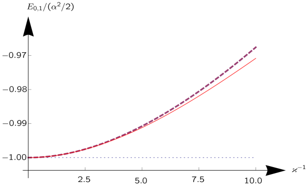
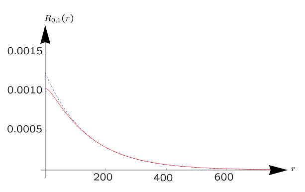
Figure 1: The energy level $E_{\ell,n}(\varkappa)$ of the ground state ($\ell=0$, $n=1$) plotted against the Bopp length $\varkappa^{-1}\in(0,10)$. The upper bound (46) and the lower bound (34) are shown also (as a dashed line and as a dotted line, respectively).

Figure 2: Radial wave function $R^{(\varkappa)}_{\ell,n}(r)$ for the ground state ($\ell=0$, $n=1$) with $\varkappa^{-1}=10$ (solid) and, for the sake of comparison, with $\varkappa^{-1}=0$ (dashed).

We now turn to the case $n=2$. In the case $\ell=0$ we use the same numerical method as for the ground state. The results are shown in Figs. 4 and 4.

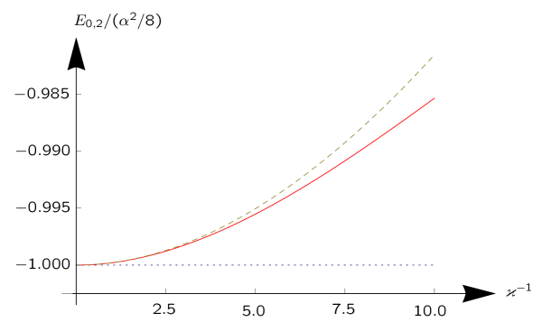
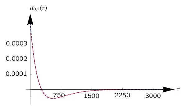
Figure 3: The energy level $E_{\ell,n}(\varkappa)$ for $\ell=0$ & $n=2$ versus $\varkappa^{-1}$. Upper bound (46) and lower bound (34) are shown as a dashed line and as a dotted line, respectively.

Figure 4: Radial wave function $R^{(\varkappa)}_{\ell,n}(r)$ for $\ell=0$ & $n=2$ with $\varkappa^{-1}=10$ (solid) and $\varkappa^{-1}=0$ (dashed). The two curves are optically barely distinguishable (near the origin).

To deal with the case $\ell=1$ is more cumbersome. As the centrifugal potential in the Schrödinger equation (29) is singular at $r=0$, the equation cannot be numerically solved by giving initial conditions at $r=0$. Therefore we give initial conditions at $r=10^{-7}$ and shoot for the solution with $u(r)=0$ and $u(r)\to 0$ for $r\to\infty$ by varying the energy and the initial conditions. The results are shown in Figs. 6 and 6.

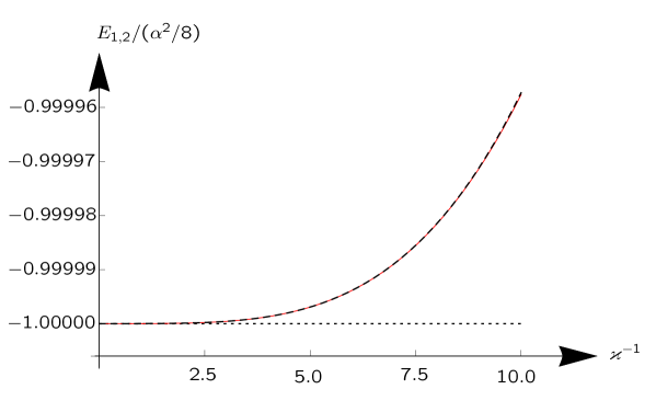
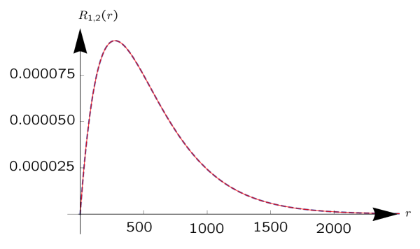
Figure 5: The energy level $E_{\ell,n}(\varkappa)$ for $\ell=1$ & $n=2$ versus $\varkappa^{-1}$. The upper bound (46) (dashed) and the lower bound (34) (dotted) are shown as well.

Figure 6: Radial wave function $R^{(\varkappa)}_{\ell,n}(r)$ for $\ell=1$ & $n=2$ with $\varkappa^{-1}=10$ (solid) and $\varkappa^{-1}=0$ (dashed). The two curves are virtually indistinguishable by the naked eye.

Figures 2, 4, and 6 reveal that the upper bound (46) is a very good approximation for the numerically computed energy for all values of $\varkappa^{-1}\leq 5$; for $E_{1,2}(\varkappa)$ this is even true over the entire interval $0<\varkappa^{-1}<10$. This tendency of increased accuracy with increasing $\ell$ is directly reflected in our upper bound (46), which becomes closer to the Coulomb eigenvalues with increasing $\ell$.

Figures 4 and 6 also reveal that $E_{1,2}(\varkappa)$ changes much less with $\varkappa^{-1}$ than $E_{0,2}(\varkappa)$. As a consequence, the well-known fact that the singlet state ($\ell=0$) and the triplet state ($\ell=1$) have the same Schrödinger energy when $\varkappa^{-1}=0$ no longer holds when $\varkappa^{-1}>0$; more precisely, $E_{0,2}(\varkappa)>E_{1,2}(\varkappa)$ for $\varkappa^{-1}\neq 0$.

The fact that $E_{0,2}(\varkappa)>E_{1,2}(\varkappa)$ for $\varkappa^{-1}\neq 0$ means that the BLTP interaction gives rise to a $\varkappa$-dependent splitting of the Lyman-$\alpha$ line (i.e., of the spectral line that corresponds to the transition from the $(n=2)$ level to the $(n=1)$ level) already with the non-relativistic Schrödinger Hamiltonian. From our numerically computed energy values we can calculate the separation

$$\Delta E(\varkappa):=\big{(}E_{0,2}(\varkappa)-E_{0,1}(\varkappa)\big{)}-\big{(}E_{1,2}(\varkappa)-E_{0,1}(\varkappa)\big{)}=E_{0,2}(\varkappa)-E_{1,2}(\varkappa)$$ (47)

of these two Lyman-$\alpha$ components. In Fig. 7 the result is plotted versus $\varkappa^{-1}$. Both energy differences $E_{1,2}(\varkappa)-E_{0,1}(\varkappa)$ and $E_{0,2}(\varkappa)-E_{0,1}(\varkappa)$ are measurable: The first one corresponds to the two dominant components of the Lyman-$\alpha$ line coming from the by far most likely spontaneous transitions from the $n=2$ to the $n=1$ level, namely from the $2{}^{2}\!P_{\frac{1}{2}}$ state to the $1{}^{2}\!S_{\frac{1}{2}}$ state and from the $2{}^{2}\!P_{\frac{3}{2}}$ state to the $1{}^{2}\!S_{\frac{1}{2}}$ state. These transitions have been routinely observed for more than a century. The second one is more difficult to observe; the single-photon transition from the $2S$ to the $1S$ state is forbidden for spinless particles in spherically symmetric potentials, i.e., it can be realised as a single-photon transition only if the electron spin is taken into account, and even then it has a very low transition probability. However, it has been observed and measured with high accuracy as a two-photon transition, see Parthey et al. [20].

Except for a subtlety which we have to discuss (see next section), the default criterion for acceptable $\varkappa$-modifications of the theoretical hydrogen spectrum would be that the differences are not larger than the measurement uncertainty of the empirical spectra. As a figure of merit for the latter we may use the fine structure splitting of the Lyman-$\alpha$ line which is usually explained as a relativistic quantum-mechanical effect. It has been calculated in the Born–Oppenheimer approximation by replacing the Schrödinger equation with the Dirac equation for an electron in the Coulomb field of an infinitely massive proton. This Dirac energy eigenvalue spectrum is identical with the Sommerfeld fine-structure formula except for its angular momentum labelling; see Ref. 19 for an illuminating analysis. The fine-structure splitting of the Lyman-$\alpha$ line is essentially due to the different spin-orbit coupling strength of the $2\,{}^{2}\!S_{\frac{1}{2}}$/$2\,{}^{2}\!P_{\frac{1}{2}}$ and $2\,{}^{2}\!P_{\frac{3}{2}}$ states; recall that the energies of the $2\,{}^{2}\!S_{\frac{1}{2}}$ and $2\,{}^{2}\!P_{\frac{1}{2}}$ states coincide in this Dirac spectrum. The numerical result, which is well confirmed by observation, for the two transition frequencies of the Lyman-$\alpha$ line is $\nu_{1}\approx 2.466060\times 10^{15}\mathrm{Hz}$ and $\nu_{2}\approx 2.466072\times 10^{15}\mathrm{Hz}$ which, in our units, corresponds to an energy difference of $\Delta E_{\mathrm{fine}}\approx 1.85\times 10^{-6}\alpha^{2}$. This value is marked in Figure 7 as a dashed line. The fact that a BLTP modification of the hydrogen spectrum has not been observed so far requires that the $\Delta E(\varkappa)$ from (47) must be small in comparison to $\Delta E_{\mathrm{fine}}$. From Figure 7 we read that this criterion requires $\varkappa^{-1}$ to be significantly smaller than $0.25$.

This is the upper bound we get from evaluating the difference of the two Lyman-$\alpha$ transition energies as given in the middle line of (47). As an alternative, we may view $\Delta E(\varkappa)$ as the direct transition energy from the ($n=2,\ell=0$) level to the ($n=2,\ell=1$) level. In the standard theory with $\varkappa^{-1}=0$ this transition is possible because the energy of the $2^{2}S_{1/2}$ state differs from the $2^{2}P_{1/2}$ state by the Lamb shift. The latter has been measured by Lamb and Retherford [21] in 1947 and theoretically calculated, on the basis of quantum electrodynamics, by Bethe [22] in the same year, with the result that the transition frequency is about 1 GHz. In our dimensionless units this corresponds to a transition energy of $\Delta E_{\mathrm{Lamb}}\approx 1.50\times 10^{-7}\alpha^{2}$, see the dotted line in Figure 7. As the observed value of the Lamb shift is in agreement with the theoretically predicted one, to within the present measuring accuracy, we may conclude that $\Delta E(\varkappa)$ must be significantly smaller than $\Delta E_{\mathrm{Lamb}}$. From Figure 7 we read that this requires $\varkappa^{-1}$ to be significantly smaller than $0.075$ which is a slightly more restrictive bound than the one from comparison with the fine structure splitting of the Lyman-$\alpha$ line.

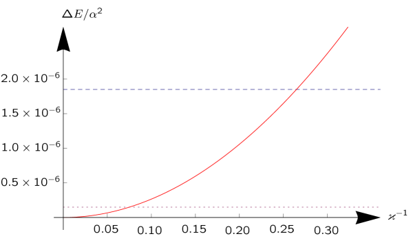
Figure 7: BLTP splitting (47) of the Lyman-$\alpha$ transition in comparison to the fine-structure splitting $\Delta E_{\mathrm{fine}}\approx 1.85\times 10^{-6}\alpha^{2}$ (dashed line) and the Lamb shift $\Delta E_{\mathrm{Lamb}}\approx 1.50\times 10^{-7}\alpha^{2}$ (dotted line).

We also numerically studied the spectrum for the much smaller and theoretically interesting value of $\varkappa^{-1}=\alpha_{S}/2$ mentioned in Remark 2.3. For this value of $\varkappa^{-1}$ we find a splitting of the Lyman-$\alpha$ line of $\Delta E\approx 3.5\times 10^{-10}\alpha^{2}$, see Fig. 8. This splitting is almost four orders of magnitude smaller than the empirical fine-structure splitting and about three orders of magnitude smaller than the Lamb shift, which would seem to be acceptable. Whether this is so will be analyzed in the next section.

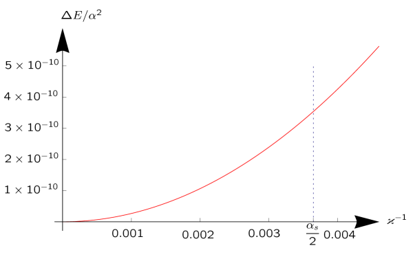
Figure 8: BLTP splitting (47) of the Lyman-$\alpha$ transition for $\varkappa^{-1}=\alpha_{\mbox{\tiny{S}}}/2\approx 1/274\approx 0.0036$.

3 Spectroscopic constraints on $\varkappa$

In the preceding section we have calculated the BLTP splitting of the Lyman-$\alpha$ transition (47) in the (spinless) Schrödinger spectrum. This splitting is caused entirely by the fact that an electron in the $\ell=0,n=2$ state is more likely to be close to the nucleus than an electron in the $\ell=1,n=2$ state, and the influence of nonzero $\varkappa^{-1}$ is largest at short distance. Thus, if one now proceeds along the lines of the usual relativistic perturbation argument, i.e. switching to the two-body Pauli equation to take electron and proton spin into account and then adding the various relativistic correction terms — in particular the spin-orbit term —, then this nonrelativistic BLTP-induced splitting would modify the usual Lyman-$\alpha$ fine structure. All three levels, $2\,{}^{2}\!S_{\frac{1}{2}}$, $2\,{}^{2}\!P_{\frac{1}{2}}$, and $2\,{}^{2}\!P_{\frac{3}{2}}$ should be lifted a little bit, yet the $2\,{}^{2}\!S_{\frac{1}{2}}$ level much more than $2\,{}^{2}\!P_{\frac{1}{2}}$ and $2\,{}^{2}\!P_{\frac{3}{2}}$ levels, the latter presumably still showing essentially the same fine-structure splitting as for the Coulomb case. By fine-tuning $\varkappa$ one may be able to achieve that the $2\,{}^{2}\!S_{\frac{1}{2}}$ and $2\,{}^{2}\!P_{\frac{3}{2}}$ levels coincide, so that energetically again there would be only two different $n=2$ fine-structure levels. Such a fine-tuning of $\varkappa$ based on just two levels would most likely be visible in a distortion of the $n=3$ fine structure, and thus be unacceptable. In any event, even for the fine-tuned $n=2$ levels their changed degeneracy would now lead to a noticeably different hyperfine structure. This line of argument leads to the conclusion that $\varkappa^{-1}$ must be significantly smaller than $0.25$, see Fig. 7.

We thus come to discuss the special value $\varkappa^{-1}=\alpha_{\mbox{\tiny{S}}}/2$. We already noted that for this $\varkappa$ value the Lyman-$\alpha$ splitting predicted by the Schrödinger eigenvalue problem with BLTP interaction, (23), is almost four orders of magnitude smaller than the observed fine-structure splitting, and would thus seem acceptable. However, the precision with which the Lyman-$\alpha$ transition energy itself has been measured — and computed perturbatively with the “standard model of hydrogen” — is so impressive that the influence of a $\varkappa^{-1}=\alpha_{\mbox{\tiny{S}}}/2$ is still too big for being in agreement with empirical data.

Explicitly, for comparison with experiments we concentrate on the transition from the $(n=2,\ell=0)$ level to the $(n=1,\ell=0)$ level of hydrogen. The transition frequency has been measured with the help of two-photon spectroscopy by Parthey et al. [20] as 2466061413187035 Hz with an absolute uncertainty of 10 Hz. By multiplication with Planck’s constant, a frequency uncertainty of 10 Hz corresponds to an energy uncertainty of $4.1\times 10^{-17}\mathrm{keV}$. After dividing by the rest energy of the electron we find that our dimensionless energy $E_{0,2}-E_{0,1}$ is known with an absolute uncertainty of $\approx 8\times 10^{-20}$.

Even though we would need the relativistic “BLTP hydrogen” spectrum of a point electron and a finite-size proton in order to make a definitive comparison, we can still extract a tentative bound on $\varkappa$ by assuming that the $\varkappa$-induced spectral line shifts in a relativistic model of a point electron bound to a finite-size proton are comparable in magnitude to those computed here with the non-relativistic Schrödinger model of a point electron bound to a point proton. Thus, we write the $\varkappa$-dependent theoretical Lyman-$\alpha$ transition energy as $E_{0,2}(\varkappa)-E_{0,1}(\varkappa)=E_{0,2}(\infty)-E_{0,1}(\infty)+\delta E(\varkappa)$ and demand that $\varkappa$ is large enough so that the $\varkappa$-induced fine structure splitting $\delta E(\varkappa)$ can be ignored. From our numerical calculations we find that $|\delta E(\varkappa)|>10^{-19}$ if $\varkappa^{-1}>3\times 10^{-6}$. We conclude that present-day spectroscopic precision measurements restrict the Bopp length $\varkappa^{-1}$ to values smaller than $3\times 10^{-6}$. Recall that we give $\varkappa^{-1}$ in units of the (reduced) Compton wave length $\lambda_{\mbox{\tiny{C}}}$ of the electron. So $\varkappa^{-1}$ is restricted to values at least two orders of magnitude smaller than the so-called classical electron radius, and thus also at least two orders of magnitude smaller than the empirical proton radius.

One might suspect that finite proton size effects will invalidate our conclusion, but this is not the case. To estimate the influence of the finite proton size, consider the extreme model in which the proton’s electric charge is uniformly distributed over a spherical shell of radius ${r}_{\rm{pr}}$. The BLTP interaction of such a charge distribution with a point electron is easily computed (cf. Ref. 23 for balls),

$$V_{\varkappa}(r)=-\alpha\frac{\min\left(\frac{r}{{r}_{\rm{pr}}},1\right)-\frac{{e^{-\varkappa|r-{r}_{\rm{pr}}|}-e^{-\varkappa(r+{r}_{\rm{pr}})}}}{2\varkappa\,{r}_{\rm{pr}}}}{r};$$ (48)

in the limit $\varkappa\to\infty$ the $\varkappa$-dependent contributions in (48) vanish and one obtains the familiar Coulomb interaction $-\frac{\alpha}{r}$ for $r>{r}_{\rm{pr}}$ and $-\frac{\alpha}{{r}_{\rm{pr}}}$ for $r\leq{r}_{\rm{pr}}$.

Now recall that our analytical upper bounds on the numerically computed eigenvalues turned out to be very accurate for “point-proton hydrogen” when $\varkappa\,{r}_{\rm{pr}}>1$ (say). The reason is easy to understand: even though the coupling constant ($\alpha$) is the same for the Coulomb and the Yukawa term in the BLTP interaction (cf. footnote 1), the Yukawa term is a form perturbation of the Schrödinger operator with pure Coulomb interaction in the sense of Kato (see Ref. 17); note though that this does not invoke an expansion in powers of $\varkappa^{-1}$. Its contribution can be made arbitrarily small by making $\varkappa$ large enough. Therefore the usual first-order perturbation theory formalism (proceding as if there was a small coefficient in front of the Yukawa term) will give the dominant correction to the Coulombic interaction spectrum. For “point proton hydrogen” this is precisely our term (35) which, when added to the Coulombic eigenvalues, produces the upper bound on the BLTP-type eigenvalues.

This form perturbation argument does not rely on having a point electron interacting with a point proton; it applies equally well when a point electron interacts with a spherical shell proton. Finally, recall that the radial wave functions $R^{(\infty)}_{\ell,n}(r)$ for $n\in\{1,2\}$ vary appreciably only on the length scale of the Bohr radius, while on the length scale of the proton radius ${r}_{\rm{pr}}$ they are essentially constant; this is true for the “point proton hydrogen” as well as for “spherical-shell proton hydrogen.” For $\ell=0$ and $n=1$, resp. $n=2$, these two $S$ states take non-zero values at the origin (the $n=2$ state somewhat smaller than the $n=1$ state), whereas for $\ell=1$ and $n=2$ this $P$ state vanishes at the origin. Thus to estimate the leading order effect when “switching on $\varkappa$,” it suffices to simply inspect the area between the graphs of $r^{2}V_{\varkappa}(r)$ and $r^{2}V_{\infty}(r)$, see Fig. 9 for when $\varkappa\,{r}_{\rm{pr}}=5$.

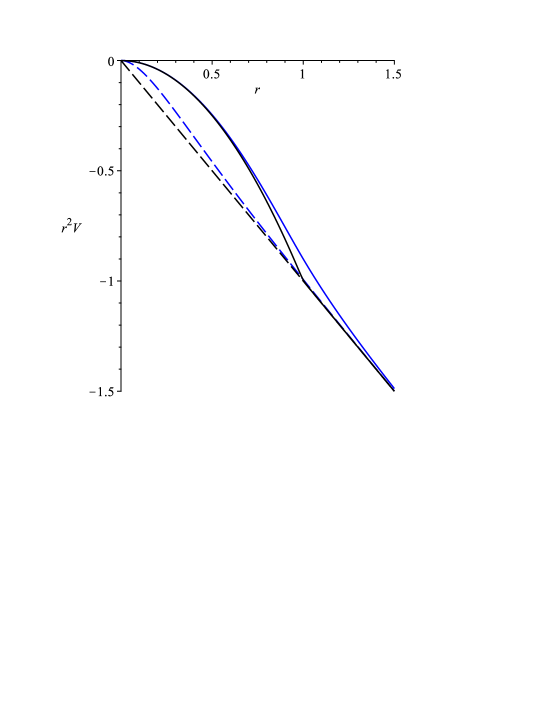
Figure 9: Shown is $r^{2}V(r)$ (up to a constant factor) versus $r$ (in units of the proton radius ${r}_{\rm{pr}}$) for a point electron interacting with a point proton (dashed lines), or with a spherical shell proton (continuous lines), once with $V$ the Coulomb (black) and once with $V$ the BLTP interaction for $\varkappa\,{r}_{\rm{pr}}=5$ (blue).

Fig. 9 suggests that replacing a point proton by a finite size proton will not significantly alter the effects on the spectrum caused by a change from a Coulomb to a BLTP interaction. We computed that the area between the two continuous curves (obtained with the spherical shell proton model) is almost exactly as large as the area between the two dashed curves (obtained with the point proton model), both when $\varkappa\,{r}_{\rm{pr}}=5$ and when $\varkappa\,{r}_{\rm{pr}}=100$.

We conclude that finite size effects of the proton will not likely invalidate our analysis that spectral data restrict $\varkappa^{-1}$ to values at least two orders of magnitude smaller than the empirical proton radius ${r}_{\rm{pr}}$.

4 Summary and Outlook

4.1 Summary

In the present paper we have studied the Schrödinger spectrum of a hydrogen atom when the conventional Coulomb pair energy between a point electron and a point proton is replaced by its Bopp–Landé–Thomas–Podolsky modification. We have obtained rigorous upper and lower bounds on the eigenvalues, and we have numerically computed a few low lying eigenvalues as functions of the Bopp length parameter $\varkappa^{-1}$. Based on our comparison of the theoretical curves with empirical data on the Lyman-$\alpha$ transition we have concluded that $\varkappa^{-1}$ has to be smaller than about $3\times 10^{-6}$ (reduced) Compton wave lengths of the electron for the theoretical spectrum not to disagree with the experimental results.

Converted to SI units, $\lambda_{\mbox{\tiny{C}}}\approx 3.86\times 10^{-13}\,\mathrm{m}$, so our limit $\varkappa^{-1}\lessapprox 3\times 10^{-6}\lambda_{\mbox{\tiny{C}}}$ means that $\varkappa^{-1}$ cannot be bigger than $\approx 10^{-18}\,\mathrm{m}$. Curiously, this is comparable to the currently available bound $R\lessapprox 10^{-18}\,\mathrm{m}$ on the size of the electron deduced in Ref. 24 from experimental data and quantum field-theoretical considerations.

Our “non-relativistic bound” on $\varkappa$ also means that the old idea of “a purely electromagnetic origin of the electron’s inertial mass,” see Refs. 1, 2, 25, 26, and 27, is untenable in BLTP electrodynamics, for it would require $\varkappa^{-1}=e^{2}/2{m}_{\rm{el}}c^{2}$ (or $\alpha_{\mbox{\tiny{S}}}/2$ in our dimensionless units), i.e. half the so-called “classical electron radius,” in flagrant violation of our non-relativistic bound on $\varkappa$. Indeed, a Bopp length $\varkappa^{-1}\approx 10^{-18}$m or less implies that the electrostatic Maxwell-BLTP field energy of a point electron is much larger than its empirical rest energy ${m}_{\rm{el}}c^{2}$. If, as assumed in all “renormalized theories” of the electron, the empirical rest mass of a physical electron is the sum of its bare rest mass and its electrostatic field energy, then in BLTP electrodynamics the electron has to be assigned a negative bare rest mass.

4.2 Outlook

It should be possible to refine our study of the influence of the Bopp–Landé–Thomas–Podolsky vacuum law of electromagnetism on the hydrogen spectrum by replacing the Schrödinger with the Pauli equation for hydrogen such that both electron and proton spin are incorporated. It is also possible to take the finite size of the proton into account in some more realistic model manner than the spherical shell proton model discussed at the end of section 3. Relativistic corrections should also be perturbatively computable. Unfortunately, a non-perturbative truly Lorentz-covariant study of the hydrogen spectrum, involving some version of a “two-body Dirac operator,” has been an elusive goal with the standard Maxwell vacuum law, and this is not going to improve by improving the vacuum law; for the time being a study of the Dirac spectrum of “BLTP hydrogen” in the Born–Oppenheimer approximation should be possible. We expect that such studies will only yield a refinement of our conclusions but no significant changes. In particular, our lower bound on $\varkappa$ obtained from discussing the Schrödinger spectrum of hydrogen is so far removed from the theoretical value obtained by demanding a vanishing bare rest mass of the electron, that we expect that all these studies will suggest a negative bare rest mass of the electron in BLTP electrodynamics.

It is an interesting question whether other modifications of the electromagnetic vacuum law, for instance the Born–Infeld law [28], also require a negative bare rest mass of the electron to be compatible with empirical spectroscopic data. The influence of the Born–Infeld nonlinearity on the theoretical hydrogen spectrum has already been investigated by various authors, see Refs. 29, 30, 31, 32 and 33, using various approximations, leading to different conclusions. The road block is the formidable Born–Infeld nonlinearity, which in the electrostatic limit reduces to the Born nonlinearity[27]. If the point charges are replaced by sufficiently smeared out charges a convergent explicit series expansion to solve the static problem has been constructed in Ref. 34, but the algorithm does not apply to point charges. A unique two-point charge solution to the electrostatic Born–Infeld equations is known to exist[35], but the nonlinearity has so far stood in the way of finding a sufficiently accurate and efficient computation of the electrostatic pair-energy of two point charges. Once this technical obstacle has been overcome the road is paved for a systematic study of the Born–Infeld effects on the Schrödinger, Pauli, and Dirac spectra of hydrogen.

References

- [1] F. Bopp, Eine lineare Theorie des Elektrons, Annalen Phys. (Leipzig) 430, 345–384 (1940).
- [2] A. Landé A and L. H. Thomas, Finite self-energies in radiation theory. Part II, Phys. Rev. 60, 514–523 (1941).
- [3] B. Podolsky, A generalized electrodynamics. Part I: Non-quantum, Phys. Rev. 62, 68–71 (1942).
- [4] B. Podolsky and P. Schwed, A review of generalized electrodynamics, Rev. Mod. Phys. 20, 40–50 (1948).
- [5] J. Gratus, V. Perlick and R. W. Tucker, On the self-force in Bopp–Podolsky electrodynamics, J. Phys. A: Math. Theor. 48, 435401 (2015).
- [6] M. K.-H. Kiessling and A. S. Tahvildar-Zadeh, Bopp–Landé–Thomas–Podolsky electrodynamics as initial value problem, Rutgers Univ. preprint, in preparation (2019).
- [7] J. Kvasnica, A possible estimate of the elementary length in electromagnetic interactions, Czech. J. Phys. 10, 625–627 (1960).
- [8] R. R. Cuzinatto, C. A. M. de Melo, L. G. Medeiros and P. J. Pompeia, How can one probe Podolsky electrodynamics? Int. J. Modern Phys. A 26, 3641–3651 (2011).
- [9] H. Hellmann, A new approximation method in the problem of many electrons, J. Chem. Phys. 3, 61 (1935).
- [10] H. Hellmann, Einführung in die Quantenchemie, (Franz Deuticke, Leipzig, 1937).
- [11] J. Adamowski, Bound eigenstates for the superposition of the Coulomb and the Yukawa potentials, Phys. Rev. A 31, 43–50 (1985).
- [12] P. Amore and F. Fernández, On an approximation to the Schrödinger equation with the Hellmann potential, (arXiv:1411.4871v1, 2014).
- [13] G. Vanden Berghe, V. Fack and H. E. De Meyer, Numerical methods for solving radial Schrödinger equations, J. Comput. Appl. Math. 28, 391–401 (1989).
- [14] C. A. Bonin, R. Bufalo, B. M. Pimentel and G. E. R. Zambrano, Podolsky electromagnetism at finite temperature: Implications on the Stefan-Boltzmann law, Phys. Rev. D 81, 025003 (2010).
- [15] A. Accioly and E. Scatena, Limits on the coupling constant of higher-derivative electromagnetism, Mod. Phys. Lett. A 25, 269–276 (2010).
- [16] M. Reed and B. Simon, Fourier Analysis, Self-Adjointness (Methods of Modern Mathematical Physics II), (Acad. Press, Orlando, 1975).
- [17] M. Reed and B. Simon, Analysis of Operators (Methods of Modern Mathematical Physics IV), (Acad. Press, Orlando, 1978).
- [18] M. Abramowitz and I. Stegun, Handbook of Mathematical Functions 9th ed, (Dover, New York, 1972).
- [19] S. Keppeler, Semiclassical quantisation rules for the Dirac and Pauli equations, Annals Phys. (NY) 304, 40–71 (2003).
- [20] C. G. Parthey et al., Improved measurement of the hydrogen 1S-2S transition frequency, Phys. Rev. Lett. 107, 203001 (2011).
- [21] W. E. Lamb and R. C. Retherford, Fine structure of the hydrogen atom by a microwave method, Phys. Rev. 72, 241 (1947).
- [22] H. Bethe, The electromagnetic shift of energy levels, Phys. Rev. 72, 339 (1947).
- [23] M. K.-H. Kiessling and J. K. Percus, Hard sphere fluids with chemical self-potentials, J. Math. Phys. 51, 015206 (2010).
- [24] S. J. Brodsky and S. D. Drell, Anomalous magnetic moment and limits on fermion substructure, Phys. Rev. D 22, 2236–2243 (1980).
- [25] H. A. Lorentz, Weiterbildung der Maxwellschen Theorie: Elektronentheorie, Encyklopädie d. Mathematischen Wissenschaften , Art. 14, 145–280 (1904).
- [26] M. Abraham, Prinzipien der Dynamik des Elektrons, Phys. Z.4, 57–63, Annalen Phys. 10, 105–179 (1903).
- [27] M. Born, Modified field equations with a finite radius of the electron, Nature 132, 282 (1933).
- [28] M. Born and L. Infeld, Foundation of the new field theory, Proc. Roy. Soc. London A 144, 425–451 (1934).
- [29] G. Heller and L. Motz, Averages over portions of configuration space, Phys. Rev. 46, 502–505 (1934).
- [30] J. Rafelski, L. P. Fulcher and W. Greiner, Superheavy elements and an upper limit to the electric field strength, Phys. Rev. Lett. 27, 958–961 (1971).
- [31] G. Soff, J. Rafelski and W. Greiner, Lower bound to limiting fields in nonlinear electrodynamics, Phys. Rev. A7, 903–907 (1973).
- [32] H. Carley and M. K.-H. Kiessling, Nonperturbative calculation of Born–Infeld effects on the Schrödinger spectrum of the hydrogen atom, Phys. Rev. Lett. 96, 030402 (1–4) (2006).
- [33] J. Franklin and T. Garon, Approximate calculations of Born–Infeld effects on the relativistic hydrogen spectrum, Phys. Lett. A 375, 1391–1395 (2011).
- [34] H. Carley and M. K.-H. Kiessling, Constructing graphs over with small prescribed mean-curvature, Math. Phys. Anal. Geom. 18, 25pp (DOI 10.1007/s11040-015-9177-6, 2015).
- [35] M. K.-H. Kiessling, On the quasi-linear elliptic PDE in physics and geometry, Commun. Math. Phys. 314, 509–523 (2012); Correction: Commun. Math. Phys. 364, 825–833 (2018).