Numerical evolution of shocks in the interior of Kerr black holes

Abstract

We numerically solve Einstein’s equations coupled to a scalar field in the interior of Kerr black holes. We find shock waves form near the inner horizon. The shocks grow exponentially in amplitude and need not be axisymmetric. Observers who pass through the shocks experience exponentially large tidal forces and are accelerated exponentially close to the speed of light.

I Introduction

The no-hair theorem postulates that the exterior geometry of black holes is completely described by the black hole’s mass, charge and angular momentum via the Kerr-Newman metric. The origin of this lies in the fact that perturbations near the event horizon can either be absorbed by the event horizon or radiated to infinity, allowing the near horizon geometry to relax. In fact the no-hair theorem should also hold just inside the event horizon as well, since just inside the event horizon of the Kerr-Newmann metric, all light rays propagate deeper into the interior. However, inside the inner horizon of the Kerr-Newmann geometry, light rays need not propagate deeper into the interior, meaning there is no mechanism for perturbations to relax and the no-hair theorem does not apply there.

The interior geometry of black holes has been most widely studied for Reissner-Nordström black holes Penrose:1968ar ; Simpson:1973ua ; HISCOCK1981110 ; PhysRevD.20.1260 ; Poisson:1989zz ; PhysRevD.41.1796 ; PhysRevLett.67.789 ; 0264-9381-10-6-006 ; Brady:1995ni ; Burko:1997zy ; Hod:1998gy ; Burko:1997fc ; Eilon:2016osg ; 10.2307/3597235 ; Marolf:2011dj . This is due to the fact that one can impose spherical symmetry, greatly simplifying calculations. One striking result is the presence of gravitational shock waves Marolf:2011dj ; Eilon:2016osg , which form along the outgoing branch of the inner horizon . The formation mechanism of the shocks essentially lies in the fact that all outgoing light rays between the event and inner horizons of the Reissner-Nordström geometry asymtotote to the inner horizon at late times. This means that outgoing radiation between the inner and event horizons — which can always be excited via scattering of infalling radiation — becomes localized to an arbitrarily thin shell as time progresses. This thin shell of radiation has a dramatic effect on infalling geodesics passing through it. Firstly, via Raychauhuri’s equation, it follows that radial null geodesics propagate from the shock to the central singularity over an exponentially small affine parameter. Likewise, upon passing through the shock, time-like radial observers are dramatically accelerated, experiencing exponentially large tidal forces, and encounter the central singularity an exponentially short proper time later. For a solar mass black hole, the proper time interval between passing through the shock and smashing into the central singularity becomes Plackian milliseconds after the black hole forms. Hence infalling observers encounter a curvature brick wall at the shock, where the curvature increases from its approximate Reissner-Nordström value to infinity over Planckian proper times.

For Kerr black holes (or more generally Kerr-Newman black holes) outgoing light rays between the event and inner horizons also asymptote to the inner horizon at late times. Hence, it is natural to expect gravitational shocks to form in the interior of rotating black holes Marolf:2011dj . In the present work we study the evolution of shocks in Kerr black holes by numerically solving Einstein’s equations coupled to a scalar field. We study both axisymmetric and non-axisymmetric solutions. Like Reissner-Nordström black holes, we find shocks form near the outgoing leg of the inner horizon. In addition to solving Einstein’s equations numerically, we also solve them analytically with a derivative expansion in the vicinity of the shocks and find excellent agreement with the numerics. Like shocks in Reissner-Nordström black holes, we find that shocks in rotating black holes dramatically affect infalling geodesics passing through them. In particular, infalling time-like observers passing through the shocks are accelerated exponentially close to the speed of light and experience exponentially large tidal forces.

II Setup

We numerically solve Einstein’s equations coupled to a massless real scalar field $\Psi$. The equations of motion read

$$R^{\mu\nu}-{\textstyle\frac{1}{2}}Rg^{\mu\nu}=8\pi T^{\mu\nu},$$ (1)

and

$$D^{2}\Psi=0,$$ (2)

where $D_{\mu}$ is the covariant derivative operator and

$$T_{\mu\nu}=D_{\mu}\Psi D_{\nu}\Psi-{\textstyle\frac{1}{2}}g_{\mu\nu}(D\Psi)^{2},$$ (3)

is the scalar stress tensor.

Our numerical evolution scheme is detailed in Chesler:2013lia . Here we outline the salient details. We employ a characteristic evolution scheme where the metric takes the form

$$\!ds^{2}=-2Adv^{2}{+}2dvd\lambda+r^{2}h_{ab}(dx^{a}{-}F^{a}dv)(dx^{b}{-}F^{b}dv),$$ (4)

with $x^{a}=\{\theta,\varphi\}$ where $\theta$ is the polar angle and $\varphi$ is the azimuthal angle. The two dimensional angular metric $h_{ab}$ satisfies $\det h_{ab}=\sin^{2}\theta$, meaning the function $r$ is an areal coordinate. Lines of constant time $v$ and angles $\theta,\varphi$ are radial null infalling geodesics. The radial coordinate $\lambda$ is an affine parameter for these geodesics. Correspondingly, the metric (4) is invariant under the residual diffeomorphism

$$\lambda\to\lambda+\xi(v,\theta,\varphi),$$ (5)

where $\xi$ is arbitrary. We fix $\xi$ such that the inner horizon of the stationary Kerr geometry is located at

$$\lambda=\lambda_{-}=1.$$ (6)

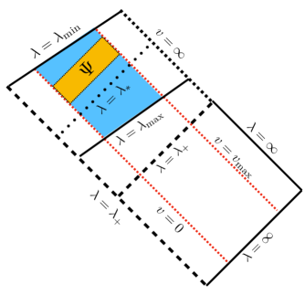
Figure 1: A Penrose diagram showing our computational domain, which is represented by the blue shaded region. Our radial coordinate $\lambda$ is the affine parameter for infalling radial geodesics, two of which are shown as the red dashed lines. The event horizon is located at $\lambda=\lambda_{+}$. The scalar field $\Psi$ (yellow shaded region) is localized inside the event horizon between $\lambda_{\rm min}(v)$ and $\lambda_{\rm max}(v)$, which are spacelike surfaces which at late times asymtotote to $\lambda=1$, the location of the inner horizon of the Kerr geometry. The outgoing null surface $\lambda=\lambda_{*}$ is employed as a matching surface in our analytic calculations below.

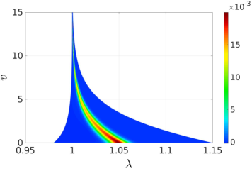
Figure 2: Evolution of the scalar field $\Psi$ in the equatorial plane for spin $a=0.9$. The inner and outer boundaries of the shaded region represent $\lambda_{\rm min}(v)$ and $\lambda_{\rm max}(v)$. As time progresses the scalar field becomes localized at $\lambda=1$.

Requisite initial data at $v=0$ consists of the scalar field $\Psi$ and the angular metric $h_{ab}$. The remaining components of the metric are determined by initial value constraint equations Chesler:2013lia . Perhaps the most natural initial data is that where a rotating black hole is formed dynamically via gravitational collapse. Another option would be to start with a Kerr initial data and allow infalling radiation to perturb the geometry inside the event horizon at $\lambda=\lambda_{+}$. A third option is to start with Kerr initial data and add a perturbation inside the event horizon. To study the evolution of shocks, it is sufficient to consider the last option, as this offers several computational advantages. First, limiting perturbations to the interior of the black hole means that one can restrict the computational domain to the interior of the black hole. Second, since no energy or angular momentum can be radiated to infinity, the mass and spin of the black hole remain constant. Because the geometry outside the inner horizon should be stable, this means that at late times the position of the inner horizon must approach that of the unperturbed Kerr geometry at $\lambda=1$. In our coordinate system this ultimately means that at late times one must have $A\to 0$ at $\lambda=1$. Having the inner horizon approach constant $\lambda$ is useful, since shocks are expected to form there.

We employ the Kerr metric for initial $h_{ab}$. For initial scalar data we choose

$$\!\!\!\!\!\!\Psi={\textstyle\frac{1}{50}}e^{-(\lambda-\lambda_{0})^{2}/2\sigma^{2}}\left\{1+\zeta\,{\rm Re}[y^{10}(\theta,\varphi){+}y^{11}(\theta,\varphi)]\right\},$$ (7)

where $y^{\ell m}$ are spherical harmonics and $\zeta$ is a parameter controlling the degree of non-axisymmetry in the initial data. We choose $\lambda_{0}$ and $\sigma$ such that $\Psi$ is localized between $\lambda=1$ and $\lambda=\lambda_{+}$ and exponentially small at our outer computational boundary. We fix the Kerr mass parameter $M=1$ and spin $a=0.9,0.95$ and $0.99$ and evolve until $v_{\rm max}=9/\kappa$ with $\kappa$ the surface gravity of inner horizon of the unperturbed Kerr black hole. For a = $0.9$, $0.95$ we set $(\lambda_{0},\sigma)=(1.05,1/150)$ while for $a=0.99$ we set $(\lambda_{0},\sigma)=(1.01,1/500)$. For axisymmetric initial data we set $\zeta=0$ and for non-axisymmetric initial data we set $\zeta=1/4$.

We employ a time dependent radial computational domain $\lambda_{\rm min}(v)\leq\lambda\leq\lambda_{\rm max}(v)$. $\lambda_{\rm min}(v)$ and $\lambda_{\rm max}(v)$ will be surfaces which at late times asymtotote to $\lambda=1$ from below and above respectively. See Fig. 1 for a Penrose diagram illustrating our computational domain. We choose

$$\!\!\!\frac{d\lambda_{\rm max}}{dv}=\min\limits_{\theta,\varphi}A\,|_{\lambda=\lambda_{\rm max}}, \frac{d\lambda_{\min}}{dv}={\max\limits_{\theta,\varphi}}\,A\,|_{\lambda=\lambda_{\rm min}}.$$ (8)

These choices mean that the surfaces $\lambda_{\rm min}(v)$ and $\lambda_{\rm max}(v)$ are either spacelike or null. This in turn means that no information can propagate from inside $\lambda_{\rm min}$ through $\lambda_{\rm min}$. At $\lambda_{\rm max}$, where the scalar field is exponentially small, we impose the boundary condition that the geometry is that of Kerr. This is allowed since no signal from inside $\lambda_{\rm max}$ can ever reach $\lambda_{\rm max}$.

Our discretization scheme is nearly identical to that in Chesler:2018txn . To discretize the equations of motion we make a linear change of coordinates from $\lambda$ to $z\in(-1,1)$ via

$$\lambda=a(v)z+b(v),$$ (9)

where

$$a(v) = {\textstyle\frac{1}{2}(\lambda_{\rm max}(v)-\lambda_{\rm min}(v))},$$ (10a)

$$b(v) = {\textstyle\frac{1}{2}(\lambda_{\rm max}(v)+\lambda_{\rm min}(v))}.$$ (10b)

Following Chesler:2013lia , we expand the $z$ dependence of all functions in a pseudo-spectral basis of Chebyshev polynomials. We employ domain decomposition in $z$ direction with 30 equally spaced domains, each containing 8 points.

For the $(\theta,\varphi)$ dependence we employ a basis of scalar, vector and tensor harmonics. These are eigenfunctions of the covariant Laplacian $-\nabla^{2}$ on the unit sphere. The scalar eigenfunctions are just spherical harmonics $y^{\ell m}$. There are two vector harmonics, $\mathcal{V}_{a}^{s\ell m}$ with $s=1,2$, and three symmetric tensor harmonics, $\mathcal{T}_{ab}^{s\ell m}$, $s=1,2,3$. Explicit representations of these functions are easily found and read oldref

$$\mathcal{V}_{a}^{1\ell m} = {\textstyle\frac{1}{\sqrt{\ell(\ell+1)}}}\nabla_{a}y^{\ell m},$$ (11a)

$$\mathcal{V}_{a}^{2\ell m} = {\textstyle\frac{1}{\sqrt{\ell(\ell+1)}}}\epsilon_{a}^{\ b}\nabla_{b}y^{\ell m},$$ (11b)

$$\mathcal{T}_{ab}^{1\ell m} = {\textstyle\frac{H_{ab}}{\sqrt{2}}}y^{\ell m},$$ (11c)

$$\mathcal{T}_{ab}^{2\ell m} = {\textstyle\frac{1}{\sqrt{\ell(\ell+1)(\ell(\ell+1)/2-1)}}}\epsilon_{(a}^{\ \ c}\nabla_{b)}\nabla_{c}y^{\ell m},$$ (11d)

$$\mathcal{T}^{3\ell m}_{ab} = {\textstyle\frac{1}{\sqrt{\ell(\ell+1)(\ell(\ell+1)/2-1)}}}[\nabla_{a}\nabla_{b}+{\textstyle\frac{\ell(\ell+1)}{2}}H_{ab}]y^{\ell m},\ \ \ \ \ \ \$$ (11e)

where $\epsilon_{a}^{\ b}$ has non-zero components $\epsilon_{\theta}^{\ \varphi}=\csc\theta$ and $\epsilon_{\varphi}^{\ \theta}=-\sin\theta$, and $H_{ab}={\rm diag}(1,\sin^{2}\theta)$ is the metric on the unit sphere. The scalar, vector and tensor harmonics are orthonormal and complete.

We expand the metric and scalar field as follows,

$$g_{00}(v,z,\theta,\varphi) = \sum_{\ell m}\alpha^{\ell m}(v,z)y^{\ell m}(\theta,\varphi),$$ (12a)

$$g_{0a}(v,z,\theta,\varphi) = \sum_{s\ell m}\beta^{s\ell m}(v,z)\mathcal{V}^{s\ell m}_{a}(\theta,\varphi),$$ (12b)

$$g_{ab}(v,z,\theta,\varphi) = \sum_{s\ell m}\gamma^{s\ell m}(v,z)\mathcal{T}^{s\ell m}_{ab}(\theta,\varphi),$$ (12c)

$$\Psi(v,z,\theta,\varphi) = \sum_{\ell m}\chi^{\ell m}(v,z)y^{\ell m}(\theta,\varphi).$$ (12d)

Derivatives in $\{\theta,\varphi\}$ can be taken by differentiating the scalar, vector and tensor harmonics.

In order to efficiently transform between real space and mode space, we employ a Gauss-Legendre grid in $\theta$ with $\ell_{\rm max}+1$ points. Likewise, we employ a Fourier grid in the $\varphi$ direction with $2\ell_{\rm max}+1$ points. These choices allow the transformation between mode space and real space to be done with a combination of Gaussian quadrature and Fast Fourier Transforms.

We truncate the expansions (12) at maximum angular momentum $\ell_{\rm max}=100$. For axisymmetric simulations we also truncate at azimuthal quantum number $m_{\rm max}=0$. For non-axisymmetric simulations we truncate at $m_{\rm max}=20$.

Figure 3: $r^{\prime}$ in the equatorial plane at several times for $a=0.9$. The $*$ denote location of the maximum of $\Psi$ at the corresponding time. A shock in $r^{\prime}$ is evident. Outside the shock, $r^{\prime}$ approaches its Kerr value while inside $r^{\prime}$ grows in time.

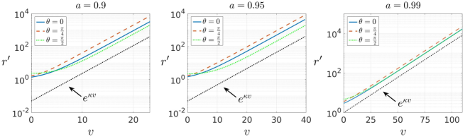
Figure 4: $r^{\prime}|_{\lambda=1}$ for axisymmetric simulations with spin $a=0.9,0.95$ and $0.99$.

III Results and discussion

We begin by presenting results for axisymmetric simulations. In Fig. 2 we plot the scalar field $\Psi$ as a function of time $v$ and radial coordinate $\lambda$ in the equatorial plane for spin $a=0.9$. The inner and outer boundaries of the shaded region correspond to the curves $\lambda_{\rm min}(v)$ and $\lambda_{\rm max}(v)$ and reflect our time-dependent computational domain. As time progresses the scalar wave packet propagates inwards towards $\lambda=1$, becoming increasingly narrower in the process while staying roughly constant in magnitude. As the scalar wave packet approaches $\lambda=1$, the metric at $\lambda>1$ approaches that of Kerr.

The localization of the scalar wave packet to $\lambda=1$ results in large $\lambda$ derivatives of the metric at $\lambda\leq 1$. A useful metric component to study is the areal coordinate $r$, which is related to the volume element via $\sqrt{-g}=r^{2}\sin\theta$. In Fig. 3 we plot $r^{\prime}|_{\lambda=1}$ in the equatorial plane at several times, again for spin $a=0.9$. Here and below

$${}^{\prime}\equiv\partial_{\lambda}.$$ (13)

The $*$ in the figure denote the maximum of $\Psi$ at the corresponding time. As is evident from the figure, there is a dramatic change in $r^{\prime}$ near the scalar maxima. In other words, there is a shock in $r^{\prime}$. Exterior to the shock $r^{\prime}$ is well approximated by its Kerr value. The change in $r^{\prime}$ across the shock grows with time.

In Fig. 4 we plot $r^{\prime}|_{\lambda=1}$ as a function of $v$ for several values of $\theta$ and for $a=0.9,0.95$ and $0.99$. Also included in each plot is $e^{\kappa v}$ where

$$\kappa=\frac{1}{2}\left(\frac{1}{M-\sqrt{M^{2}-a^{2}}}-\frac{1}{M}\right),$$ (14)

is the surface gravity of the inner horizon of the corresponding Kerr solution. For $a=0.9,0.95$ and $0.99$ we have $\kappa\approx 0.386,0.227$ and $0.0821$, respectively. Our numerics are consistent with the scaling $r^{\prime}\sim e^{\kappa v}$.

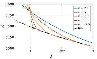
Figure 5: The Kretschmann scalar $K$ in the equatorial plane at several times for an axisymmetric simulation with $a=0.9$. The $*$ denote location of the maximum of the scalar wave packet at the corresponding time. Exterior to the wave packet $K$ is well described by its Kerr value. At $\lambda=1$ $K$ is nearly constant but $K^{\prime}$ grows with time.

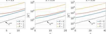
Figure 6: $|K^{\prime}||_{\lambda=1}$ evaluated at several polar angles for axisymmetric simulations with spin $a=0.9,0.95$ and $0.99$.

We now turn to the curvature. In Fig. 5 we plot the Kretschmann scalar

$$K\equiv R^{\mu\nu\alpha\beta}R_{\mu\nu\alpha\beta},$$ (15)

as a function of $\lambda$ in the equatorial plane at several times for the same simulation shown in Fig. 4. The $*$ denote the location of the maximum of $\Psi$ at the corresponding time. Exterior to the scalar wave packet, $K$ is well approximated by its Kerr value. A prominent feature of Fig. 5 is that $K^{\prime}$ grows dramatically with time just inside the wave packet. In Fig. 6 we plot $|K^{\prime}||_{\lambda=1}$ as a function of $v$ at several values of $\theta$ for the same simulations shown in Fig. 4. Also included in the plots is $e^{\kappa v}$. Our numerics are consistent with the scaling $|K^{\prime}||_{\lambda=1}\sim e^{\kappa v}$. Evidently, $\lambda=1$ becomes a curvature brick wall at late times, with a shock in $K$ developing there.

The geometry in the vicinity of the shocks can be studied perturbatively Marolf:2011dj . To account for the rapid $\lambda$ dependence, we introduce a bookkeeping parameter $\epsilon\ll 1$ and assume the scalings

$$\partial_{\lambda}\sim 1/\epsilon, A\sim\epsilon.$$ (16)

The scaling $A\sim\epsilon$ is necessary to have $A^{\prime}=O(1)$, which itself is necessary to have a finite surface gravity at $\lambda=1$ as $v\to\infty$. We then solve the Einstein-scalar system in the region $\lambda<\lambda_{*}$ with $\lambda_{*}=1+O(\epsilon)$. A convenient choice of matching surface $\lambda=\lambda_{*}$ is an outgoing null sheet exterior to the scalar wavepacket, as shown in Fig. 1.

On the surface $\lambda=\lambda_{*}$ we impose the boundary condition that the geometry is that of Kerr and that the scalar field vanishes. At leading order in $\epsilon$ we therefore need the inner horizon values of the Kerr metric. In our coordinate system, at the inner horizon of Kerr we have

$$A|_{\lambda=1}=0, A^{\prime}|_{\lambda=1}=-\kappa, F^{a}|_{\lambda=1}=\Omega\delta^{a\phi},$$ (17)

where

$$\Omega=\frac{\sqrt{M^{2}-a^{2}}+M}{2aM},$$ (18)

is the angular velocity of the inner horizon. It follows that for the Kerr solution

$$D_{+}g_{\mu\nu}|_{\lambda=1}=0,$$ (19)

where

$$D_{+}\equiv\partial_{v}+A\partial_{\lambda}+F^{a}\partial_{a},$$ (20)

is the directional derivative along outgoing null geodesics.

At leading order in $\epsilon$ the $(\mu,\nu)=(v,a)$ component of the Einstein equations (1) reduces to

$$F^{\prime a}=0.$$ (21)

The boundary conditions (17) therefore implies

$$F^{a}=\Omega\delta^{a\phi}.$$ (22)

With the solution (22), at leading order in $\epsilon$ the $(\mu,\nu)=(v,\lambda)$ and $(a,b)$ components of Einstein’s equations reduce to

$$0 =(rD_{+}r)^{\prime},$$ (23a)

$$0 =\textstyle\left[\delta^{c}_{a}\delta^{d}_{b}-\frac{1}{2}h^{cd}h_{ab}\right](rD_{+}h_{cd})^{\prime}+D_{+}rh^{\prime}_{ab},$$ (23b)

$$0 =\textstyle A^{\prime\prime}+\frac{1}{4}h^{ab}h^{\prime}_{bc}h^{cd}D_{+}h_{da}-\frac{2r^{\prime}D_{+}r}{r}$$ (23c)

$$+8\pi\Psi^{\prime}D_{+}\Psi,$$

where $h^{ab}$ is the inverse of $h_{ab}$. Likewise, at leading order in $\epsilon$ the scalar equation of motion (2) reduces to

$$(rD_{+}\Psi)=-\Psi^{\prime}D_{+}r.$$ (24)

Eqs. (23a), (23b) and (24) are just radial wave equations for $r$, $h_{ab}$ and $\Psi$. Imposing the boundary conditions that the geometry exterior to the shell is that of Kerr is tantamount to imposing the boundary conditions that there is no infalling radiation through the shell, which is what (19) states. With the boundary condition (19), Eqs. (23a), (23b) and (24) have the solutions

$$D_{+}r=0, D_{+}\Psi=0, D_{+}h_{ab}=0.$$ (25)

These first order wave equations state that excitations in $r$, $\Psi$ and $h_{ab}$ are transported along outgoing null geodesics tangent to $D_{+}$. Substituting (25) into (23c) and employing the boundary conditions (17), we secure

$$A=-\kappa\lambda.$$ (26)

With the solutions (26) and (22) and the definition of $D_{+}$ in (20), the first order system (25) is solved by

$$r(v,\lambda,\theta,\varphi) =\rho(e^{\kappa v}(\lambda-1),\theta,\varphi-\Omega v),$$ (27a)

$$\Psi(v,\lambda,\theta,\varphi) =\psi(e^{\kappa v}(\lambda-1),\theta,\varphi-\Omega v),$$ (27b)

$$h_{ab}(v,\lambda,\theta,\varphi) =\mathcal{H}_{ab}(e^{\kappa v}(\lambda-1),\theta,\varphi-\Omega v),$$ (27c)

where $\rho$, $\psi$ and $\mathcal{H}_{ab}$ are arbitrary functions. Note that curves with $e^{\kappa v}(\lambda-1)$, $\theta,$ and $\varphi-\Omega v$ all constant are simply outgoing null geodesics near $\lambda=1$. These geodesics spiral in towards $\lambda=1$ at angular frequency $\Omega$, which is due to frame dragging, and eventually terminate at $\lambda=1$ as $v\to\infty$. The value of the fields on these geodesics is constant. Since the $\lambda$ dependence comes in the combination $e^{\kappa v}(\lambda-1)$, it follows that $e^{-\kappa v}$ plays the role of our bookkeeping parameter $\epsilon$.

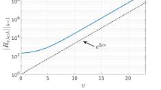
Figure 7: The Riemann tensor component $R_{v\lambda v\lambda}|_{\lambda=1}$ in the equatorial plane for an axisymmetric simulations with spin $a=0.9.$ The Riemann tensor diverges like $e^{2\kappa v}$.

The above analysis implies that as $v\to\infty$, the scalar wave packet must approach $\lambda=1$, just as seen in Fig. 2. Moreover, it immediately follows from (27) that the individual components of the Riemann tensor scale like

$$R_{\mu\nu\alpha\beta}\sim e^{2\kappa v}.$$ (28)

Indeed, in Fig. 7 we plot the component $R_{v\lambda v\lambda}|_{\lambda=1}$ in the equatorial plane for an axisymmetric simulation with spin $a=0.9$ and verify this scaling. The exponential growth in (28) reflects the fact that outgoing radiation is blue shifted by a factor of $e^{\kappa v}$, becoming exponentially localized in $\lambda$ in the process. However, owing to the fact that all excitations in (27) are purely outgoing, the curvature scalar $K$ cannot blow up exponentially, meaning all exponential factors in (15) cancel. Why must this happen? Since by construction there is no infalling radiation present, one can simply boost to the frame where the outgoing radiation is not blue shifted and the components $R_{\mu\nu\alpha\beta}$ and Kretschmann scalar are finite as $v\to\infty$. Simply put, with only outgoing radiation present, the Kretschmann scalar — and in fact all other scalars — can only depend on $\{v,\lambda,\varphi\}$ through the combinations $e^{\kappa v}(\lambda-1)$ and $\varphi-\Omega v$. It therefore follows that $K$ is finite on the shocks and that

$$r^{\prime}|_{\lambda=1}=e^{\kappa v}H(\theta,\varphi-\Omega v), K^{\prime}|_{\lambda=1}=e^{\kappa v}Q(\theta,\varphi-\Omega v),$$ (29)

for some functions $H$ and $Q$. The scaling relations (29) match those shown in Figs. 4 and 5 for our axisymmetric simulations.

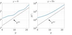
Figure 8: $|K^{\prime}||_{\lambda=1}$ in the equatorial plane for a non-axisymmtric simulation with spin $a=0.95$. The left plot is evaluated at $\varphi=0$ whereas the right is at $\varphi=\Omega v$.

The scaling relations (29) also demonstrate rotation invariance in $\varphi$ can be broken: a small non-axisymmetric perturbation in initial data results in violations of axisymmetry in $r^{\prime}$ and $K^{\prime}$ which are exponentially amplified. To demonstrate this, in Fig. 8 we plot $K^{\prime}|_{\lambda=1}$ at $\theta=\pi/2$ as a function of time for a non-axisymmetric simulation with $a=0.95$. The left figure is evaluated at $\varphi=0$ while the right figure is evaluated at $\varphi=\Omega v$. At $\varphi=0$ we see that $K^{\prime}$ grows exponentially with sinusoidal oscillations superimposed. In the rotating frame, where $\varphi=\Omega v$, the sinusoidal oscillations are not present, just as (29) requires. Evidently, the curvature brick wall at $\lambda=1$ retains angular structure contained in the initial data. Oscillating features of the curvature were also reported in Ori:2001pc .

Let us now turn to analyzing the effect of the shocks on infalling geodesics. Consider first radial infalling null geodesics with $v={\rm const}.$ The null energy condition implies that $r^{\prime\prime}/r<0$. This means that $r^{\prime}$ can only increase as $\lambda$ decreases. Since just inside the shock $r^{\prime}\sim e^{\kappa v}$, it follows that the affine distance $\Delta\lambda$ from the shock to the point $r=0$ is

$$\Delta\lambda\sim e^{-\kappa v}.$$ (30)

This reflects the fact that the shock focuses infalling light rays to $r=0$, which can also be seen from Raychaudhuri’s equation. Turning now to infalling time-like geodesics, the scaling (28) means that infalling time-like observers crossing the shocks will experience tidal forces of order $e^{2\kappa v}$. In particular, upon crossing the shocks the areal velocity will be

$$\frac{dr}{d\tau}\sim-e^{\kappa v}.$$ (31)

What then is the fate of an observer who jumps into the black hole at late times? For large enough black holes, observers need not experience any ill effects until they pass through the shocks. They will measure the local geometry to be that of Kerr, with arbitrarily small tidal forces. Upon encountering the shocks though, they will be torn apart by tidal forces and their subsequent debris will be accelerated nearly to the speed of light towards the black hole interior.

In the present paper we only considered perturbations in the interior of black holes and did not allow infalling radiation. Exterior perturbations of black holes in asymtotically flat spacetime results in infalling radiation which decays with a power law in $v$ in accords with Price’s Law Price:1972pw . For Reissner-Nordström black holes, infalling radiation results in a weak null curvature singularity developing on the ingoing leg of the inner horizon ($v=\infty$ in Fig. 1) Poisson:1989zz ; PhysRevD.41.1796 . A similar effect should happen for Kerr black holes. With infalling radiation, the exponential factors in (28) cannot be ameliorated via a boost, for a boost which compensates the $e^{\kappa v}$ blueshift of outgoing radiation will inevitably result in the infalling radiation being blue shifted by a factor of $e^{\kappa v}$. With infalling radiation present, it is therefore reasonable to expect that $K$ will blow up like $e^{2\kappa v}$. We leave the inclusion of infalling radiation for future studies.

IV Acknowledgments

This work was supported by the Black Hole Initiative at Harvard University, which is funded by a grant from the John Templeton Foundation. EC is also supported by grant 312032894 from the Deutsche Forschungsgemeinschaft. We thank Amos Ori and Peter Galison for useful comments and discussions.

References

- (1) R. Penrose, “Structure of space-time,”.
- (2) M. Simpson and R. Penrose, “Internal instability in a Reissner-Nordstrom black hole,” Int. J. Theor. Phys. 7 (1973) 183–197.
- (3) W. A. Hiscock, “Evolution of the interior of a charged black hole,” Physics Letters A 83 (1981) no. 3, 110 – 112. http://www.sciencedirect.com/science/article/pii/0375960181905089.
- (4) Y. Gürsel, I. D. Novikov, V. D. Sandberg, and A. A. Starobinsky, “Final state of the evolution of the interior of a charged black hole,”Phys. Rev. D 20 (Sep, 1979) 1260–1270. https://link.aps.org/doi/10.1103/PhysRevD.20.1260.
- (5) E. Poisson and W. Israel, “Inner-horizon instability and mass inflation in black holes,” Phys. Rev. Lett. 63 (1989) 1663–1666.
- (6) E. Poisson and W. Israel, “Internal structure of black holes,”Phys. Rev. D 41 (Mar, 1990) 1796–1809. https://link.aps.org/doi/10.1103/PhysRevD.41.1796.
- (7) A. Ori, “Inner structure of a charged black hole: An exact mass-inflation solution,”Phys. Rev. Lett. 67 (Aug, 1991) 789–792. https://link.aps.org/doi/10.1103/PhysRevLett.67.789.
- (8) M. L. Gnedin and N. Y. Gnedin, “Destruction of the cauchy horizon in the reissner-nordstrom black hole,” Classical and Quantum Gravity 10 (1993) no. 6, 1083. http://stacks.iop.org/0264-9381/10/i=6/a=006.
- (9) P. R. Brady and J. D. Smith, “Black hole singularities: A Numerical approach,” Phys. Rev. Lett. 75 (1995) 1256–1259, arXiv:gr-qc/9506067 [gr-qc].
- (10) L. M. Burko, “Structure of the black hole’s Cauchy horizon singularity,” Phys. Rev. Lett. 79 (1997) 4958–4961, arXiv:gr-qc/9710112 [gr-qc].
- (11) S. Hod and T. Piran, “Mass inflation in dynamical gravitational collapse of a charged scalar field,” Phys. Rev. Lett. 81 (1998) 1554–1557, arXiv:gr-qc/9803004 [gr-qc].
- (12) L. M. Burko and A. Ori, “Analytic study of the null singularity inside spherical charged black holes,” Phys. Rev. D57 (1998) 7084–7088, arXiv:gr-qc/9711032 [gr-qc].
- (13) E. Eilon and A. Ori, “Numerical study of the gravitational shock wave inside a spherical charged black hole,” Phys. Rev. D94 (2016) no. 10, 104060, arXiv:1610.04355 [gr-qc].
- (14) M. Dafermos, “Stability and instability of the cauchy horizon for the spherically symmetric einstein-maxwell-scalar field equations,” Annals of Mathematics 158 (2003) no. 3, 875–928. http://www.jstor.org/stable/3597235.
- (15) D. Marolf and A. Ori, “Outgoing gravitational shock-wave at the inner horizon: The late-time limit of black hole interiors,” Phys. Rev. D86 (2012) 124026, arXiv:1109.5139 [gr-qc].
- (16) P. M. Chesler and L. G. Yaffe, “Numerical solution of gravitational dynamics in asymptotically anti-de Sitter spacetimes,” JHEP 07 (2014) 086, arXiv:1309.1439 [hep-th].
- (17) P. M. Chesler and D. A. Lowe, “Nonlinear evolution of the AdS4 black hole bomb,” arXiv:1801.09711 [gr-qc].
- (18) V. D. Sandberg, “Tensor spherical harmonics on and as eigenvalue problems,” Journal of Mathematical Physics 19 (1978) no. 12, 2441–2446, https://doi.org/10.1063/1.523649.
- (19) A. Ori, “Oscillatory null singularity inside realistic spinning black holes,” Phys. Rev. Lett. 83 (1999) 5423–5426, arXiv:gr-qc/0103012 [gr-qc].
- (20) R. H. Price, “Nonspherical Perturbations of Relativistic Gravitational Collapse. II. Integer-Spin, Zero-Rest-Mass Fields,” Phys. Rev. D5 (1972) 2439–2454.