Sculpting Andromeda – made-to-measure models for M31’s bar and composite bulge: dynamics, stellar and dark matter mass

Abstract

The Andromeda galaxy (M31) contains a box/peanut bulge (BPB) entangled with a classical bulge (CB) requiring a triaxial modelling to determine the dynamics, stellar and dark matter mass. We construct made-to-measure models fitting new VIRUS-W IFU bulge stellar kinematic observations, the IRAC-3.6${\rm\mu m}$ photometry, and the disc’s H I rotation curve. We explore the parameter space for the 3.6${\rm\mu m}$ mass-to-light ratio $\left({\Upsilon_{3.6}\,\,}\!\!\right)$, the bar pattern speed (${\Omega_{\rm p}\,\,}\!\!$), and the dark matter mass in the composite bulge (${M^{\rm B}_{\rm DM}\,\,}\!\!$) within $3.2\,{\rm kpc}$. Considering Einasto dark matter profiles, we find the best models for ${\Upsilon_{3.6}\!=\!0.72\!\pm\!0.02\,{\rm M_{\odot}\,L_{\odot}^{-1}}\,}$, ${M^{\rm B}_{\rm DM}\!=\!1.2^{+0.2}_{-0.4}\times 10^{10}\,{\rm M_{\odot}}\,}$and ${\Omega_{\rm p}\!=\!40\pm 5\,{\rm km}\,{\rm s}^{\rm-1}\,{\rm kpc}^{-1}}$. These models have a dynamical bulge mass of $M_{\rm dyn}^{\rm B}\,{\!=\!}\,4.25^{+0.10}_{-0.29}\times\!10^{10}\,{\rm M_{\odot}}$ including a stellar mass of $M_{\star}^{\rm B}\,{\!=\!}\,3.09^{+0.10}_{-0.12}\times\!10^{10}\,{\rm M_{\odot}}$(73%), of which the CB has $M_{\star}^{\rm CB}\,{\!=\!}\,1.18^{+0.06}_{-0.07}\times\!10^{10}\,{\rm M_{\odot}}$(28%) and the BPB $M_{\star}^{\rm BPB}\,{\!=\!}\,1.91\pm 0.06\!\times\!10^{10}\,{\rm M_{\odot}}$(45%). We also explore models with NFW haloes finding that, while the Einasto models better fit the stellar kinematics, the obtained parameters agree within the errors. The ${M^{\rm B}_{\rm DM}\,\,}$values agree with adiabatically contracted cosmological NFW haloes with M31’s virial mass and radius. The best model has two bulge components with completely different kinematics that only together successfully reproduce the observations ($\mu_{3.6}$, $\upsilon_{\rm los},\sigma_{\rm los}$, $h3$, $h4$). The modelling includes dust absorption which reproduces the observed kinematic asymmetries. Our results provide new constraints for the early formation of M31 given the lower mass found for the classical bulge and the shallow dark matter profile, as well as the secular evolution of M31 implied by the bar and its resonant interactions with the classical bulge, stellar halo and disc.

1 Introduction

The Andromeda galaxy (M31, NGC224) is the closest neighbouring massive spiral galaxy, presenting us a unique opportunity to study in depth the dynamics of disc galaxy substructures, such as classical bulges and bars, the latter found in approximately 70 per cent of the disc galaxies in the local Universe (Menendez-Delmestre et al., 2007; Erwin, 2017). In addition, our external perspective more easily proves a global view of M31 in comparison to the Milky Way, while as a similar mass disk galaxy, it allows us to place our home galaxy in context.

Historically, M31’s triaxial bulge has been mostly addressed as a classical bulge, while generally the bar component has been only qualitatively considered in the modelling of its stellar dynamics. However, an accurate dynamical estimation of the mass distribution of the stellar and the dark matter in the bulge must take into account the barred nature of M31’s central regions (Lindblad, 1956). More recent observations better quantify the triaxiality of the bulge which is produced by its box/peanut bulge ($\rm BPB$) component (Beaton et al., 2007; Opitsch et al., 2017), a situation similar in many aspects to the Milky Way’s box/peanut bulge (Shen et al., 2010; Wegg & Gerhard, 2013; Bland-Hawthorn & Gerhard, 2016). The M31 $\rm BPB$ is in addition entangled with a classical bulge ($\rm CB$) component (Athanassoula & Beaton, 2006). The $\rm CB$ is much more concentrated than the $\rm BPB$, with the two components contributing with $\,{\!\sim\!}\,$ 1/3 and $\,{\!\sim\!}\,$ 2/3 of the total stellar mass of the bulge respectively, as shown by Blaña et al. (2017, hereafter B17).

Each substructure in M31 can potentially teach us about the different mechanisms involved in the formation and the evolution of the whole galaxy. In particular, the properties of the $\rm CB$ component of M31 can give us information about the early formation epoch. Current galaxy formation theories consider classical bulges as remnants of a very early formation process, such as a protogalactic collapse, and/or as remnants of mergers of galaxies that occurred during the first gigayears of violent hierarchical formation (Toomre, 1977; Naab & Burkert, 2003; Bournaud et al., 2005). On the other hand, the massive $\rm BPB$ of M31 provides us information about the evolution of the disc, as box/peanut bulges are formed later from the disc material. Box/peanut bulges in N-body models are triaxial structures formed through the buckling instability of the bar, which typically lasts for $\lesssim 1\,{\rm Gyr}$, generating a vertically thick structure (Combes et al., 1990; Raha et al., 1991). Recent observations of two barred galaxies also show evidence of their bars in the buckling process (Erwin & Debattista, 2016). Box/peanut bulges are frequent being found in 79 per cent of massive barred local galaxies ($M_{\star}\gtrsim 10^{10.4}\,{\rm M_{\odot}}$, Erwin & Debattista, 2017). Note that box/peanut bulges are sometimes referred as box/peanut pseudobulges, however not to be confused with discy pseudobulges, which are formed by gas accreted into the centres of disc galaxies (Kormendy, 2013).

Moreover, on even longer time-scales, box/peanut bulges and bars can interact through resonances with the disc and thereby redistribute its material, generating for example surface brightness breaks, as well as ring-like substructures (Buta & Crocker, 1991; Debattista et al., 2006; Erwin et al., 2008; Buta, 2017). Bars also transfer their angular momentum to the spheroid components, such as classical bulges (Saha et al., 2012, 2016), stellar haloes (Perez-Villegas et al., 2017) and dark matter haloes (Athanassoula & Misiriotis, 2002), changing their dynamical properties. Furthermore, Erwin & Debattista (2016) show also with observations that classical bulges can coexist with discy pseudobulges and box/peanut bulges building composite bulges, a scenario that has also been reproduced in galaxy formation simulations (Athanassoula et al., 2016). This makes M31 a convenient laboratory to test formation theories of composite bulges and to better understand their dynamics.

To understand the formation and the evolution of Andromeda, and to accurately compare it with galaxy formation simulations, it is imperative to first determine the contribution and the properties of each of the substructures, such as their masses and sizes, as well as the dark matter distribution. In the outer disc region the gas kinematics constrain the dark matter distribution (Chemin et al., 2009; Corbelli et al., 2010). However, in the centre, the gas may not be in equilibrium due to the triaxial potential generated by the bar. Therefore, we model the stellar kinematics taking into consideration the triaxial structure of the $\rm BPB$. Opitsch (2016, hereafter O16) and Opitsch et al. (2017, hereafter O17) obtained kinematic observations of exquisite detail using the integral field unit (IFU) VIRUS-W (Fabricius et al., 2012), completely covering the classical bulge, the $\rm BPB$ and most of the projected thin or planar bar. In this paper we use these kinematic observations to fit a series of made-to-measure models that allow us to find constraints for the stellar and dark matter mass within the bulge region, as well as other dynamical parameters such as the pattern speed of the $\rm BPB$ and the thin bar.

This paper is ordered as follows: Section 2 describes the observational data, its implementation, and the made-to-measure modelling of M31. Section 3 shows the results of the models that are separated in two main parts. In the first, Section 3.1, we present the main results of the parameter search exploration. In the second part, in Section 3.2, we present the properties of the best model and we compare it with the M31 observations. In Section 4 we conclude with a summary and a discussion of the implications of our findings.

2 Modelling the bulge of M31

Most dynamical models for the bulge of M31 assume a spherical or an oblate geometry for the bulge (Ruiz, 1976; Kent, 1989; Widrow et al., 2003; Widrow & Dubinski, 2005; Block et al., 2006; Hammer et al., 2010), making the mass estimations in the centre less accurate due to the barred nature of this galaxy. N-body barred galaxy models can represent the bulge and the bar of M31 much better. However, finding an N-body model that exactly reproduces all the properties of the M31 substructures is very difficult, because N-body models depend on their initial conditions and on the bar formation and buckling instabilities, evolving with some degree of stochasticity. Therefore, here we use the Made-to-measure (M2M) method to model the bulge of M31 (Syer & Tremaine, 1996, hereafter ST96). This method can model triaxial systems and therefore it is the most suitable approach to model M31’s bar.

In the following sections we describe our technique that implements the M2M method to fit the kinematic and the photometric observations, which allows us to determine the main dynamical properties of the M31 composite bulge: the pattern speed of the bar (${\Omega_{\rm p}\,\,}$), the stellar mass-to-light ratio of the bulge in the 3.6${\rm\mu m}$ band (${\Upsilon_{3.6}\,\,}$) and the dark matter mass within the bulge (${M^{\rm B}_{\rm DM}\,\,}$).

2.1 Made-to-measure method

We use the program nmagic that implements the M2M method to fit N-body models to observations (De Lorenzi et al., 2007; De Lorenzi et al., 2008; Morganti & Gerhard, 2012; Portail et al., 2015; Portail et al., 2017a). In the original implementation of the M2M method (ST96) the potential and the model observables are calculated from the initial mass distribution of the particles, where their masses are then optimised to match observations, requiring a mass distribution of the particles that is close to the final model. In the nmagic implementation the potential is periodically recomputed to generate a system that is gravitationally self-consistent.

A discrete model observable is defined for a system with $N$ particles with phase-space time ($t$) depending coordinates $\vec{z}_{i}\left(t\right)\,{\!=\!}\,\left(\vec{r}_{i},\vec{v}_{i}\right)$ as:

$$y\left(t\right)=\sum_{i\,{\!=\!}\,1}^{N}\,K_{i}\left(\vec{z}_{i}\left(t\right)\right)\,w_{i}$$ (1)

where $K_{i}$ is a known kernel that is used to calculate the distribution moments, $w_{i}$ is the weight of each particle that contributes to the observable, corresponding here to the particle’s mass. We increase the effective number of particles implementing an exponential temporal smoothing with timescale $\tau_{\rm s}$, obtaining the smoothed observable $y_{\tau}$.

The observational data is composed by $j$ observations (e.g. $j$ number of pixels in an image), and by $k$ different sets of observations; here we work with one set of photometric observations and four sets of kinematic observations. Therefore, we generalise to $Y_{j}^{k}$ observations with $Y_{\rm err}\,{}_{j}^{k}$ errors, and by observing the model similarly we have $y_{\tau}\,{}_{j}^{k}$ temporally smoothed model observables and $K_{i\,j}^{k}$ kernels . The deviation between the model observables and the observations is defined by the delta

$$\Delta_{j}^{k}\left(t\right)=\frac{y_{\tau}\,{}_{j}^{k}\left(t\right)-Y_{j}^{k}}{Y_{\rm err}\,{}_{j}^{k}}$$ (2)

and therefore the sum in time of $\left(\Delta_{j}^{k}\right)^{2}$ is the chi-square $\chi^{2}\,_{j}{}^{k}$ of the temporal smoothed model observables and the observations.

The heart of the M2M method is the algorithm that determines how the weights of the particles change in time during the iterative fit to the observations. Here we use the “force-of-change” (FOC) defined by ST96 as:

$$\frac{dw_{i}}{dt}=\epsilon\,w_{i}\,\partial_{w_{i}}F$$ (3)

where $\epsilon$ is a constant adjusting the strength of the FOC. This relation is a gradient ascent algorithm that maximises $F$ in the space of the weights, defined in NMAGIC as

$$F=-\frac{1}{2}\chi^{2}_{\rm tot}+\mu S$$ (4)

Here the first term is just the total chi-square

$$\chi^{2}_{\rm tot}=\sum_{k,j}\lambda_{k}\,\chi^{2}\,_{j}{}^{k}$$ (5)

where $\chi^{2}\,_{j}{}^{k}=\left(\Delta_{j}^{k}\right)^{2}$, and $\lambda_{k}$ are $k$ constants that balance the contributions between different $k$ sets of observables (Long & Mao, 2010; Portail et al., 2015). The term $S$ is an “entropy” introduced by ST96 that forces the weights of the particle distribution to remain close to their initial distribution, defined here as in Morganti et al. (2013); Portail et al. (2017a).

$$S=\sum_{i}w_{i}\left(1-\ln\frac{w_{i}}{\hat{w}_{i}}\right)$$ (6)

where the “priors” $\hat{w}_{i}$ are the averages of the weights of each of the stellar particle types. The entropy term also forces the model to slowly change its initial 3D mass density distribution. The factor $\mu$ balances the contribution between the entropy term and the chi-square term (De Lorenzi et al., 2007). Introducing the previous terms in equation 3 we have now the FOC equation

$$\frac{dw_{i}}{dt}=-\epsilon\,w_{i}\left[\mu\ln\left(\frac{w_{i}}{\hat{w}_{i}}\right)+\sum_{k}\lambda_{k}\sum_{j}\left(K_{i\,j}^{k}+w_{i}\,\partial_{w_{i}}K_{i\,j}^{k}\right)\frac{\Delta_{j}^{k}}{Y_{\rm err}\,{}_{j}^{k}}\right]$$ (7)

With the observables that we define later the differential term becomes zero ($\partial_{w_{i}}K_{i\,j}^{k}\,{\!=\!}\,0$).

2.2 Inputs to the M2M modelling from B17: initial N-body model and projection angles

The M2M modelling requires an initial input particle model that contains the orbits required to construct a new model that successfully matches the observations. Therefore, we use the best matching particle model for the M31 bulge from B17, i.e. Model 1, which comes from a set of 72 N-body models built with a box/peanut bulge ($\rm BPB$) component and a classical bulge ($\rm CB$) component with different masses and scale lengths. These models evolved from a Hernquist density profile for the classical bulge and another for the dark matter halo, where none of these components have initial rotation. During these simulations the initial disc forms a bar that later buckles forming a $\rm BPB$, but leaving bar material in the plane which is the thin bar. The thin bar is aligned with the $\rm BPB$ extending beyond this. We reserve the term “bar” for whole structure of the thin bar and the $\rm BPB$ together. The bar and disc particles have the same label, as the bar evolved from the initial disc. The bar is entangled with the $\rm CB$, where both structures evolve due to the transfer of angular momentum from the bar to the $\rm CB$ and the dark matter halo as well, gaining both rotation. The light of the $\rm CB$ bulge and the $\rm BPB$ dominate in the centre, and therefore no stellar halo component is included. The number of particles used for the $\rm CB$, bar and disc and the dark matter halo are $N_{\rm CB}\,{\!=\!}\,10^{6}$, $N_{\rm bar+disc}\,{\!=\!}\,10^{6}$ and $N_{\rm halo}\,{\!=\!}\,2\times 10^{6}$.

Model 1 (see B17) has a concentrated $\rm CB$ with a 3D half-mass radius $r_{\rm half}^{\rm CB}\,{\!=\!}\,0.53\,{\rm kpc}$ $(140\,{\rm arcsec})$ and a $\rm BPB$ with a 3D semimajor axis of $r^{\rm BPB}\,{\!=\!}\,3.2\,{\rm kpc}\,(840\,{\rm arcsec})$ and a half-mass radius of $r_{\rm half}^{\rm BPB}\,{\!=\!}\,1.3\,{\rm kpc}$ $(340\,{\rm arcsec})$. Within the radius $r^{\rm BPB}$, B17 measure a stellar mass of the composite bulge of $M^{\rm B}_{\star}\,{\!=\!}\,3.3\times 10^{10}\,{\rm M_{\odot}}$, where the $\rm CB$ and the $\rm BPB$ have $\,{\!\sim\!}\,1/3$ and $\,{\!\sim\!}\,2/3$ of the bulge total stellar mass, respectively. They estimate a stellar mass-to-light ratio in the 3.6${\rm\mu m}$ of ${\Upsilon_{3.6}\,\,}_{\rm B17}\,{\!=\!}\,0.813\,{\rm M_{\odot}\,L_{\odot}^{-1}}$. The initial dark matter halo mass within 51$\,{\rm kpc}$ is $3.8\times 10^{11}\,{\rm M_{\odot}}$ and within $r^{\rm BPB}$ is ${M^{\rm B}_{\rm DM}\,\,}\,{\!=\!}\,0.7\times 10^{10}\,{\rm M_{\odot}}$. This model has a bar pattern speed of ${\Omega_{\rm p}\,\,}\,{\!=\!}\,38\,{\rm km}\,{\rm s}^{\rm-1}\,{\rm kpc}^{-1}$.

We tested our final results using another model from B17 as the input N-body model for the M2M fits. This model had the same initial conditions as Model 1, except for the classical bulge mass being 30 per cent higher. We found only small differences in the final fitted M2M model.

We also need to project the M2M models on the sky to calculate the model observables defined later in Section 2.3, requiring the distance to M31 $d_{\rm M31}$, the disc inclination angle $i$, the disc major axis position angle ${\rm PA}_{\rm disk}$, and the bar angle $\theta_{\rm bar}$. For this we use the same quantities adopted as in B17: $d_{\rm M31}\,{\!=\!}\,785\pm 25\,{\rm kpc}$ (McConnachie et al., 2005) (at this distance $3.8\,{\rm pc}\,{\!=\!}\,1\,{\rm arcsec}$, $1\,{\rm kpc}\,{\!=\!}\,260\,{\rm arcsec}$ and $13.7\,{\rm kpc}\,{\!=\!}\,1\degree$ on the sky), $i\,{\!=\!}\,77\degree$ (Corbelli et al., 2010), ${\rm PA}_{\rm disk}\,{\!=\!}\,38\degree$ (de Vaucouleurs, 1958), and the bar angle $\theta_{\rm bar}\,{\!=\!}\,54{\degree\!\!.}7\pm 3{\degree\!\!.}8$ measured in B17. The bar angle is defined in the plane of the disc (where the bar major axis would be aligned with the disc projected major axis for $\theta_{\rm bar}\,{\!=\!}\,0\degree$, see B17 Figure 1). Projecting $\theta_{\rm bar}$ into the sky results in an angle of $\theta_{\rm proj}\,{\!=\!}\,17{\degree\!\!.}7\pm 2{\degree\!\!.}5$ measured from the line of nodes of the disc major axis, corresponding to a position angle of ${\rm PA}_{\rm bar}\,{\!=\!}\,55{\degree\!\!.}7\pm 2{\degree\!\!.}5$. We corroborate later in Section 3.1.5 that $\theta_{\rm bar}\,{\!=\!}\,54{\degree\!\!.}7\pm 3{\degree\!\!.}8$ is the bar angle that best matches the photometry of the bulge, reproducing the bulge isophotal twist.

2.3 Fitting the photometry and IFU kinematics

In this section we describe how we prepare M31’s photometric and kinematic observational data to use as constraints for the M2M fitting with nmagic. The photometric data consist of an image of M31 from the Infrared Array Camera 1 (IRAC 1) . The kinematic data correspond to IFU observations of the bulge region of M31, and to H I rotation curves in the disc region. Consistently with the observations, we build model observables that measure the same quantities in the model and are used to fit to the equivalent data values. However, as we explain later in Section 2.8, to find our range of the best matching models we select a subsample of the fitted observations to compare them with the models. All the model observables $y_{j}^{k}$ defined here are temporally smoothed to $y_{\tau}\,{}_{j}^{k}$.

2.3.1 Photometry I: IRAC 3.6${\rm\mu m}$ observations

The imaging data that we use come from the large-scale IRAC mosaic images of M31 of the Spitzer Space Telescope (Barmby et al., 2006) kindly made available to us by Pauline Barmby. We use the IRAC 1 band that at 3.6${\rm\mu m}$ wavelength for two reasons: i) it traces well the old stars (bulk of the population) where the light is dominated by giant stars that populate the red giant branch (RGB), and ii) this band has the advantage of being only weakly affected by the dust emission or absorption (Meidt et al., 2014). The IRAC1 mosaic of Barmby et al. (2006) has pixels with size of 0.863$\,{\rm arcsec}$ and covers a region of $3{\degree\!\!.}7\times 1{\degree\!\!.}6$. We are interested in covering the inner bulge region, both the region where the $\rm CB$ dominates within $\,{\!\sim\!}\,100\,{\rm arcsec}\,(0.4\,{\rm kpc})$ in the projected radius, also where the $\rm BPB$ is at $\,{\!\sim\!}\,700\,{\rm arcsec}\,(2.7\,{\rm kpc})$ in projection. We use a resolution of 8.63$\,{\rm arcsec}$ ($32.8\,{\rm pc}$) per pixel for the image, which is a convenient scale that faithfully shows the light gradients in the central region where the transition between the $\rm CB$ and the $\rm BPB$ is. As we are interested in the scenario where the 10$\,{\rm kpc}$-ring could be connected to the outer Lindblad resonance, we include the region of the stellar disc out to $3950\,{\rm arcsec}\,(15\,{\rm kpc})$. We define an ellipse with this projected semimajor axis by fitting to the isophotes with the ellipse task in iraf. We mask the pixels of the image that are outside this 15$\,{\rm kpc}$ ellipse and proceed to fit the image. We also mask hot pixels in the image, foreground stars, and the dwarf galaxy M32. At the end of the filtering, the total number of photometric observable (pixels) used for the M2M fit is 170651.

The original image pixel values are in intensity $I\,[{\rm MJy}\,{\rm sr}^{-1}]$. The surface-brightness figures in the paper that are in $\,{\rm mag\,{\rm arcsec^{-2}}}$ are in the Vega system, and they are transformed from the original units using the 3.6${\rm\mu m}$ zero-point calibration 280.9 ${\rm Jy}$ (Reach et al., 2005). The conversion between the SB in $\,{\rm mag\,{\rm arcsec^{-2}}}$ and the luminosity $\,{\rm L_{\odot}}$ is done using the absolute solar magnitude value $M_{\odot}^{3.6}\,{\!=\!}\,3.24\,{\rm mag}$ (Oh et al., 2008), and multiplying $I$ by the pixel area $A_{\rm pixel}\,{\!=\!}\,8.63\times 8.63\,{\rm arcsec}^{2}\,{\!=\!}\,32.8\times 32.8\,{\rm pc}^{2}$.

We also require photometric error maps for the M2M modelling. Given that the M2M models are a representation of M31 in dynamical equilibrium, they cannot reproduce the observed substructures in M31 that are produced by perturbations such as spiral arms. Therefore, we include these smaller scale deviations between M31 and the models in the errors. For this we combined three types of error maps: the observational error $L_{\rm err}^{\rm obs}$, the variability between pixels $L_{\rm err}^{\rm stdv}$ and the asymmetry error $L_{\rm err}^{\rm asym}$. The first error ($L_{\rm err}^{\rm obs}$) is calculated from the square root of the sum in quadrature of the pixel error and the standard deviation for each pixel that comes from the original 0.863$\,{\rm arcsec}$ pixels. The typical $L_{\rm err}^{\rm obs}$ errors are between one and 5 per cent of the intensity depending on the pixel location in the image. This error is smaller than the variability observed between contiguous pixels and so we therefore include a second error that takes into account the pixel-to-pixel scatter. The surface-brightness image of our M2M models is smoother than the observations. We take into account this variability by including in the photometric error the standard deviation within a radius of one 8.63$\,{\rm arcsec}$-pixel around each pixel of the image, obtaining the error $L_{\rm err}^{\rm stdv}$. Finally we also include the variability observed at kiloparsec scales due to substructures like the spiral arms beyond the bar region, and the 10$\,{\rm kpc}$-ring. For this we subtract the image with the same image, but rotated 180°around the centre of the bulge, obtaining $L_{\rm err}^{\rm asym}$. The bulge is roughly symmetric making this term smaller in the bulge than in the disc region. The combined photometric error per pixel $Y_{{\rm err}}\,^{k}{}_{j}$ with $k\,{\!=\!}\,0$ is then:

$$Y_{{\rm err}}\,^{k\,{\!=\!}\,0}{}_{j}=L_{\rm err}\,{}_{j}\,{\!=\!}\,\left[\left(L_{\rm err}^{\rm obs}\,{}_{j}\right)^{2}+\left(L_{\rm err}^{\rm stdv}\,{}_{j}\right)^{2}+\left(L_{\rm err}^{\rm asym}\,{}_{j}\right)^{2}\right]^{1/2}$$ (8)

2.3.2 Photometry II: model observables and the mass-to-light ratio (${\Upsilon_{3.6}\,\,}$)

The photometric model observables consist of an array of pixels that extends from the bulge centre out to the disc until 15$\,{\rm kpc}$ along the disc major axis, where each model pixel uniquely corresponds to each observed pixel, with the same pixel size ($8.63\,{\rm arcsec}$). Each $j$th pixel measures the stellar masses $m_{i}$ of $N_{j}$ particles that pass through each pixel, which are converted to light in the 3.6${\rm\mu m}$ band using the stellar mass-to-light ratio ${\Upsilon_{3.6}\,\,}$. The total light per pixel $L_{j}$ is the photometric model observable $y_{j}^{k}$ with $k\,{\!=\!}\,0$ :

$$y_{j}^{k}=L_{j}\,{\!=\!}\,\sum_{i}^{N_{j}}\,l_{i}\,{\!=\!}\,\sum_{i}^{N_{j}}\Upsilon_{i}^{-1}\,m_{i}$$ (9)

where the light per particle ($l_{i}$) is just $\Upsilon_{i}^{-1}\,m_{i}$. We define three mass-to-light ratio parameters in the 3.6${\rm\mu m}$ band: $\Upsilon^{\rm CB}$ for the classical bulge, $\Upsilon^{\rm BPB}$ for the $\rm BPB$ and $\Upsilon^{\rm d}$ for the outer disc, which are assigned to the particles according to the relation:

$$\Upsilon_{i}=\begin{cases}\Upsilon^{\rm CB}&\text{if }i\in\text{CB}\\ \Upsilon^{\rm BPB}&\text{if }i\notin\text{CB}\wedge\ R_{i}\leq R_{\rm t}\\ \left(\Upsilon^{\rm BPB}-\Upsilon^{\rm d}\right)e^{\frac{-\left(R_{i}-R_{\rm t}\right)^{2}}{2\,R_{\rm s}^{2}}}+\Upsilon^{\rm d}&\text{if }i\notin\text{CB}\wedge\ R_{i}>R_{\rm t}\\ \end{cases}$$ (10)

where the $\rm CB$ particles are assigned $\Upsilon^{\rm CB}$ everywhere, and the bar and disc particles at the cylindrical radius $R_{i}$ are assigned $\Upsilon^{\rm BPB}$ within $R_{\rm t}$, and $\Upsilon^{\rm d}$ if they are outside this radius. The last Gaussian term provides a smooth transition of $\Upsilon_{i}$ from the value of $\Upsilon^{\rm BPB}$ to the value in the disc $\Upsilon^{\rm d}$, where $R_{\rm t}$ is the transition radius between the end of the thin bar and the disc $R_{\rm t}\,{\!=\!}\,4\,{\rm kpc}$ (B17), and $R_{\rm s}$ is the scale of the transition ($R_{\rm s}\,{\!=\!}\,1.5\,{\rm kpc}$).

In Section 2.8 we explain in more detail the different mass-to-light values that we explored, however in our fiducial M2M fits we assumed ${\Upsilon_{3.6}\,\,}\,{\!=\!}\,\Upsilon^{\rm CB}\,{\!=\!}\,\Upsilon^{\rm BPB}\,{\!=\!}\,\Upsilon^{\rm d}$. In Sections 3.1.2 and 3.1.3 we explore further different values for each component, finding only small differences compared with our range of best models. From equation 9 we have that the photometric kernel ($k\,{\!=\!}\,0$) is

$$K^{k\,{\!=\!}\,0}_{i\,j}\,{\!=\!}\,\Upsilon_{i}^{-1}$$ (11)

2.3.3 Kinematics I: M31 Bulge IFU observations

O16 and O17 obtained kinematic IFU observations of the central region of M31 using the McDonald Observatory’s 2.7-meter Harlan J. Smith Telescope and the VIRUS-W Spectrograph (Fabricius et al., 2012). They cover the whole bulge and bar region and also sample the disc out to one disc scale length along six different directions, obtaining line-of-sight velocity distribution profiles (LOSVDs). From this they calculate the four Gauss-Hermite expansion coefficient moments (Gerhard, 1993; Bender et al., 1994), and obtain kinematic maps for the velocity $\upsilon_{\rm los}$, the velocity dispersion $\sigma_{\rm los}$ and the kinematic moments $h3$ and $h4$. The velocity maps are corrected for the systemic velocity of $-300\,{\rm km}\,{\rm s}^{\rm-1}$ (de Vaucouleurs et al., 1991). Note that the light weighted mean line-of-sight velocity $\langle\upsilon\rangle_{\rm los}$ and the light weighted velocity standard deviation (or dispersion) $\langle\sigma\rangle_{\rm los}\,{\!=\!}\,\sqrt{\langle\upsilon^{2}\rangle_{\rm los}-\langle\upsilon\rangle^{2}_{\rm los}}$, differ slightly from $\upsilon_{\rm los}$ and $\sigma_{\rm los}$ when the LOSVDs deviate from a Gaussian distribution ($h3\!\neq\!0$ or $h4\!\neq\!0$ or non-zero higher moments). This is because $\upsilon_{\rm los}$ and $\sigma_{\rm los}$ are instead chosen so that the lower order Gauss-Hermite terms, $h1$ and $h2$, are zero.

We re-grid the kinematic observations into new maps with the same spatial resolution of the photometric data. The new values of $\upsilon_{\rm los}$, $\sigma_{\rm los}$, $h3$ and $h4$ are calculated from the error weighted average of the original values, leaving 13400 measurements for each kinematic variable, and therefore 53600 kinematic values in total. The re-gridded observational kinematic errors ($Y_{\rm err}^{\rm obs}\,{}_{j}^{k}$, with $k\,{\!=\!}\,1,2,3,4$) are calculated from the standard deviation of the error weighted average. Similarly to the photometry, we combined the new observational error and the error due to the variability between different kinematic pixels within one pixel radius ($Y_{\rm err}^{\rm stdv}\,{}^{k}_{j}$), obtaining a total kinematic error per observable and per set of:

$$Y_{{\rm err}}\,^{k}{}_{j}\,{\!=\!}\,\left[\left(Y_{\rm err}^{\rm obs}\,{}_{j}^{k}\right)^{2}+\left(Y_{\rm err}^{\rm stdv}\,{}^{k}_{j}\right)^{2}\right]^{1/2}.$$ (12)

2.3.4 Kinematics II: model observables

We now proceed to build the kinematic model observables. Because the kinematic observations are performed in the V band, we need to include the effects of dust in our model observables. A further description is given later in Section 3.2.3. Our dust absorption implementation consists of using M31 dust mass maps (Draine et al., 2014) converted to a V band absorption map by the dust model of Draine & Li (2007)

$$A_{\rm V}^{j}=0.74\left(\frac{\Sigma_{\rm dust}^{j}}{10^{5}\,{\rm M_{\odot}}\,\,{\rm kpc}^{-2}}\right)\,{\rm mag}\leavevmode\nobreak\ .$$ (13)

We convert this to a 3D absorption map $p^{A{\rm V}}$, deprojected as

$$p^{A{\rm V}}_{i,j}=\begin{cases}10^{-0.4\,A_{\rm V}^{j}}&\text{if }z_{i}\leq 0\,{\rm kpc}\\ 1&\text{if }z_{i}>0\,{\rm kpc}\end{cases}$$ (14)

where for simplicity we assume that the dust is located in the plane of the disk, and therefore any stellar $i$th particle that is temporarily passing behind the disc at the moment that the kinematic model observable is measured, is attenuated by the corresponding value of $p^{A{\rm V}}_{i,j}$ in the $j$th pixel.

So that the kernel of Equation 1 does not depend on weight, we desire kinematic model observables that are linear in the particle weights. Therefore, we fit the Gauss-Hermite moments of the observations, $h1\,{\!=\!}\,0$ and $h2\,{\!=\!}\,0$, instead of directly fitting $\sigma_{\rm los}$ and $\upsilon_{\rm los}$ (De Lorenzi et al., 2007). The model kinematic observables are then the light-weighted Gauss-Hermite coefficient moments, calculated as in De Lorenzi et al. (2007), but with the inclusion of dust absorption:

$$y_{j}^{k}={\rm H}k_{j}=\sum^{N_{j}}_{i}\,p^{A{\rm V}}_{i,j}\,l_{i}\,h_{n,i}\,{\!=\!}\,\sum^{N_{j}}_{i}\,p^{A{\rm V}}_{i,j}\,\Upsilon_{i}^{-1}\,m_{i}\,2\sqrt{\pi}\,u_{k}\left(\beta_{i}\right)\leavevmode\nobreak\ .$$ (15)

Here $k\,{\!=\!}\,1,2,3,4$, and $u_{k}\left(\beta_{i}\right)$ are the dimensionless Gauss-Hermite functions (Gerhard, 1993),

$$u_{k}\left(\beta_{i}\right)=\left(2^{n+1}\pi n!\right)^{-1/2}\,H_{k}\left(\beta_{i}\right)\exp\left(-\beta_{i}^{2}/2\right)$$ (16)

where $H_{k}$ are the standard Hermite polynomials, are

$$\beta_{i}=\left(\upsilon_{i}-\upsilon_{\rm los}\right)/\sigma_{\rm los}$$ (17)

where $\upsilon_{i}$ is the particle’s line-of-sight velocity. The expansion is performed with the observational values of $\sigma_{\rm los}$ and $\upsilon_{\rm los}$ so that while $h$1 and $h$2 are zero in the observations, they are in general non-zero when observing the model. From this we obtain the light weighted model observables ${\rm H1}$, ${\rm H2}$, ${\rm H3}$, and ${\rm H4}$. The corresponding kinematic kernel that changes the weights of the particles is

$$K^{k}_{i\,j}\,{\!=\!}\,p^{A{\rm V}}_{i,j}\,\Upsilon_{i}^{-1}\,2\sqrt{\pi}\,u_{k}\left(\beta_{i}\right)\leavevmode\nobreak\ .$$ (18)

Concordantly, the observational data that we fit are the Gauss-Hermite moments $h1\,{\!=\!}\,0$, $h2\,{\!=\!}\,0$, $h3$ and $h4$, which are light-weighted by the extincted light model observable

$$L_{j}^{A{\rm V}}\,{\!=\!}\,\sum_{i}^{N_{j}}\,p^{A{\rm V}}_{i,j}\,\Upsilon_{i}^{-1}\,m_{i}\leavevmode\nobreak\ .$$ (19)

This is then used to light weight the kinematic observations e.g. ${\rm H1}\,{\!=\!}\,h1\,L^{A{\rm V}}$, obtaining the observations that we fit: ${\rm H1}$, ${\rm H2}$, ${\rm H3}$ and ${\rm H4}$.

The errors for $h1$ and $h2$ are calculated from the observations $\upsilon_{\rm los}$ and $\sigma_{\rm los}$ as in van der Marel & Franx (1993); Rix et al. (1997).

$$h1_{\rm err}=\frac{1}{\sqrt{2}}\frac{\upsilon_{\rm los,err}}{\sigma_{\rm los}}; h2_{\rm err}=\frac{1}{\sqrt{2}}\frac{\sigma_{\rm los,err}}{\sigma_{\rm los}}$$ (20)

Then, the kinematic errors $h1_{\rm err}$, $h2_{\rm err}$, $h3_{\rm err}$ and $h4_{\rm err}$ are also light-weighted in the form ${\rm H1}_{\rm err}\,{}_{j}\,\,{\!=\!}\,h1_{\rm err}\,{}_{j}\,\left(L_{j}\right)^{2}\,\left(L_{j}^{A{\rm V}}\right)^{-1}$, which gives larger errors to the regions with more light extinction. From this we obtained the light weighted errors ${\rm H1_{\rm err}}$, ${\rm H2_{\rm err}}$, ${\rm H3_{\rm err}}$, ${\rm H4_{\rm err}}$. We also test our best model fit considering no dust absorption ($A_{\rm V}^{j}\,{\!=\!}\,0\,{\rm mag}$) and a constant value $A_{\rm V}^{j}\,{\!=\!}\,0.5\,{\rm mag}$.

To facilitate side-by-side comparison of the model with the observations, and also for the selection of the range of best models defined in Section 2.8, we also compute after the M2M fitting the temporally smoothed $\upsilon_{\rm los}$ and $\sigma_{\rm los}$ of the model, and use these values to calculate $h3$ and $h4$ of the model. For this we observe the model and calculate ${\rm H1}$, ${\rm H2}$, ${\rm H3}$, ${\rm H4}$ of the model using equation 15, but in equation 17 we replace $\upsilon_{\rm los}$ and $\sigma_{\rm los}$ of the observations by the mean velocity $\langle\upsilon\rangle_{\rm los}$ and the velocity standard deviation $\langle\sigma\rangle_{\rm los}$ of the model. The non-light weighted quantities are recovered dividing by $L^{A{\rm V}}_{j}$, i.e. h1=H1/$L^{A{\rm V}}_{j}$ and similarly for $h2$, $h3$, $h4$. The parametrisation of the LOSVD with the Gauss-Hermite moments dictates that the variables $\sigma_{\rm los}$ and $\upsilon_{\rm los}$ are chosen such that $h1$ and $h2$ are zero. If this is not the case we use again the approximation (van der Marel & Franx, 1993; Rix et al., 1997) to correct and replace the old values of the velocity and the dispersion ($\upsilon_{\rm o},\sigma_{\rm o}$) with the new values ($\upsilon_{\rm n},\sigma_{\rm n}$) that result in new h$1_{\rm n}$ and h$2_{\rm n}$ values closer to zero:

$$\upsilon_{\rm n}=\upsilon_{\rm o}+\sqrt{2}\,\sigma_{\rm o}h1_{\rm o}\left(\upsilon_{\rm o},\sigma_{\rm o}\right)$$ (21a)

$$\sigma_{\rm n}=\sigma_{\rm o}+\sqrt{2}\,\sigma_{\rm o}h2_{\rm o}\left(\upsilon_{\rm o},\sigma_{\rm o}\right)$$ (21b)

We repeat the previous corrections observing the model and calculating the new $h1$, $h2$, $h3$, $h4$ from the new dispersion and velocity using equation 15, repeating this iteratively until the terms $h1$ and $h2$ converge to zero or values smaller than the observational errors.

2.4 Adjusting the dark matter mass within the bulge (${M^{\rm B}_{\rm DM}\,\,}$), and fitting the H I rotation curve

Our goal is to determine the dark matter mass within 3.2$\,{\rm kpc}$ of the bulge ${M^{\rm B}_{\rm DM}\,\,}$, by exploring a vast range of values given in Section 2.8. For this we change the initial dark matter mass distribution of the input N-body model to match a target analytical profile. As we also want to explore the cusped or cored nature of the dark matter density in the central region, we consider different shapes for the target dark halo, making M2M models with two different target profiles. We consider the Einasto density profile (Einasto, 1965) which has a central core, parametrised here as:

$$\rho_{\rm DM}^{\rm EIN}\left(m\right)=\rho_{\rm E}\,\exp\left\{-\left(\frac{2}{\alpha}\right)\,\left[\left(\frac{m}{m_{\rm E}}\right)^{\alpha}-1\right]\right\}$$ (22)

where $m\,{\!=\!}\,\sqrt{x^{2}+y^{2}+(z/q)^{2}}$ is the elliptical radius for a flattening $q$, $m_{\rm E}$ is the scale length, $\rho_{\rm E}$ is the central density and $\alpha$ is the steepness of the profile. We also comte models with a Navarro-Frenk-White (NFW) dark matter mass density profile, which has a cuspy central profile (Navarro et al., 1996), parametrised here as

$$\rho_{\rm DM}^{\rm NFW}\left(m\right)=\frac{\rho_{\rm N}}{\left(m/m_{\rm N}\right)\left[1+\left(m/m_{\rm N}\right)^{2}\right]}$$ (23)

where $\rho_{\rm N}$ is the central density and $m_{\rm N}$ is the scale length.

The parameters of these target analytical profiles are determined during each M2M run similarly to Portail et al. (2017a), by fitting the dark matter halo profile together with the current stellar mass distribution to match: i) the dark matter mass enclosed within an ellipsoidal volume of the major axis of the bulge ($r^{\rm BPB}\,{\!=\!}\,m^{\rm BPB}\,{\!=\!}\,3.2\,{\rm kpc}$) is fixed to the chosen value ${M^{\rm B}_{\rm DM}\,\,}$, with ${M^{\rm B}_{\rm DM}\,\,}=\int\!\!dv\,\rho_{\rm DM}$ (or $M_{\rm DM}^{\rm B(p)}$ from the particles); and ii) that the total circular velocity of the model matches well the disc H I rotation curve data (Corbelli et al., 2010) described in Section 2.4.1.

To adjust the particle dark matter distribution to the target analytical dark matter profile we also use the M2M method (De Lorenzi et al., 2007). This is done by expanding the initial dark matter density distribution of the particles and the target analytical dark matter density profile in spherical harmonics, which are then fitted with the M2M scheme. The adaptation of the dark matter particles is performed while the photometric and the stellar kinematic observations are also being fitted.

A change in the dark matter mass profile may significantly change the total circular velocity, particularly in the disc region, affecting the orbits of the particles. This is not desirable for particles in the disc that should remain on near-circular or epicyclic orbits. To alleviate this we measure the circular velocity for a $i$th particle before and after the potential update, and then re-scale the velocity of the particle living in the old potential $\phi_{\rm old}$ to a new velocity given by the new potential $\phi_{\rm new}$ by multiplying its velocity by the factor $f_{V_{\rm c},i}$ that is the ratio between the new and the old circular velocities:

$$f_{V_{\rm c},i}=\sqrt{\vec{A}_{i}\cdot\vec{\nabla}_{A_{i}}\,\phi_{\rm new}/\vec{A}_{i}\cdot\vec{\nabla}_{A_{i}}\,\phi_{\rm old}}$$ (24)

using the spherical radius vector $\vec{A}_{i}\,{\!=\!}\,\vec{r}_{i}$ for the dark matter and $\rm CB$ particles that have a spheroidal geometric distribution, and the cylindrical radius $\vec{A}_{i}\,{\!=\!}\,\vec{R}_{i}$ for the disc particles.

2.4.1 Kinematics III: H I rotation curve

We use the de-projected azimuthally averaged H I rotation velocity curve estimated by Corbelli et al. (2010) to fit the total circular velocity of our M2M models modifying the dark matter profile for a given ${\Upsilon_{3.6}\,\,}$(see Section 2.4) . This data extend from 8.5$\,{\rm kpc}$ out to 50$\,{\rm kpc}$. We do not fit the rotation curve beyond 20$\,{\rm kpc}$, for two reasons: i) the contribution of the mass of the H I disc to the circular velocity beyond this radius becomes as important as the stellar disc (Chemin et al., 2009), and ii) the outer disc shows a warp ($R>27\,{\rm kpc}$) changing the inclination with respect to the inner part of the stellar and gaseous discs (Newton & Emerson, 1977; Henderson, 1979; Brinks, E.; Burton, 1984; Chemin et al., 2009). This region includes the 10$\,{\rm kpc}$-ring and the 15$\,{\rm kpc}$ ring structures Gordon et al. (2006); Barmby et al. (2006). We do not include the mass of the gas component in the potential as the gas mass and surface mass contribution within 20$\,{\rm kpc}$ is estimated to be less than 10 per cent of the stellar mass ($\Sigma_{\rm gas}/\Sigma_{\star}<0.1$) (Chemin et al., 2009) and, as we show later in Section 3.1.3, the choice of different dark matter profiles introduces variations larger than this.

2.5 Bar pattern speed adjustment (${\Omega_{\rm p}\,\,}$)

The pattern speed of the bar of the model found in B17 is ${\Omega_{\rm p}\,\,}\,{\!=\!}\,38\,{\rm km}\,{\rm s}^{\rm-1}\,{\rm kpc}^{-1}$. As we want to find constraints for this quantity, we also explore pattern speeds (see Section 2.8). To change the initial pattern speed, we adiabatically and linearly change its initial value to the desired final value with a certain frequency defined in Section 2.7 (see Martinez-Valpuesta, 2012; Portail et al., 2017a). This pattern speed change is performed while the kinematic and the photometric observables are fitted and the potential is frequently recalculated from the new density distribution, resulting at the end of the M2M fit in a self-consistent dynamical system.

2.6 Potential solver and orbital integration

As in Portail et al. (2017a), the NMAGIC modelling here uses the hybrid particle-mesh code from Sellwood et al. (2003) to calculate the potential from the particle mass distribution. The potential solver uses a cylindrical mesh Fourier method to calculate the potential for the disc and the bulge components (Sellwood & Valluri, 1997). Due to the disc geometry and our interest in resolving the vertical and the in plane distribution, instead of using a spherical softening, we use an oblate softening with 67$\,{\rm pc}$ in the plane and 17$\,{\rm pc}$ in the vertical direction. The potential of the particles of the dark matter component is calculated using a spherical mesh with a spherical harmonics potential solver that extends to 42$\,{\rm kpc}$ and includes terms up to the 16th order (De Lorenzi et al., 2007). The cylindrical mesh extends in the disc plane out to $R\,{\!=\!}\,10\,{\rm kpc}$ and $z\pm 3\,{\rm kpc}$ in the vertical direction, and any stellar mass particle that extends beyond the limits of this mesh is considered during the run in the spherical mesh for the calculation of the potential.

The orbits of the particles are integrated forward in time with an adaptive leap-frog algorithm using the acceleration due to the gravitational potential of all the particles. In the nmagic M2M implementation the rotating bar is kept fix in the reference frame of the potential by rotating the phase-space coordinates of all the particles around the $z$-axis at the same rate of the pattern speed of the bar, but opposite in sign (Martinez-Valpuesta, 2012; Portail et al., 2015) (note that the rotated system is still in an inertial frame).

The integration time is measured in iteration units $\,{\rm\left[it\right]}$, with a time step of $1\,{\rm\left[it\right]}\,{\!=\!}\,0.23\,{\rm Myr}$ (see B17, ). We require that the orbits always have at least 1000 steps per orbit.

2.7 M2M fitting procedure and parameters

Each M2M fitting done here with nmagic takes a total number of iterations of $T_{\rm tot}\,{\!=\!}\,80000\,{\rm\left[it\right]}$, where each fit is divided in three main phases. The first phase uses $T_{\rm obs}\,{\!=\!}\,5000\,{\rm\left[it\right]}$, and is when the temporal smoothed measurements of the model observables are calculated. The temporal smoothing scale is $\tau_{\rm s}\,{\!=\!}\,1600\,{\rm\left[it\right]}$, and it is chosen to be larger than the period (${\rm T_{orbit}}$) of a circular orbit at 5$\,{\rm kpc}$ with circular velocity $V_{c}$, which typically is $\,{\!\sim\!}\,1000\,{\rm\left[it\right]}$.

The second phase is when the M2M fitting is performed, and it takes $T_{\rm M2M}\,{\!=\!}\,50000\,{\rm\left[it\right]}$. The bar pattern speed is adjusted during this phase, starting at $T_{\rm i}^{\rm ps}\,{\!=\!}\,10000\,{\rm\left[it\right]}$ and finishing at $T_{\rm f}^{\rm ps}\,{\!=\!}\,40000\,{\rm\left[it\right]}$, with an update of the new value every $T_{\rm up}^{\rm ps}\,{\!=\!}\,3000\,{\rm\left[it\right]}$. During the second phase the total mass of the system may change. Therefore, we recalculate and update the potential from the new mass density distribution every $T_{\rm pot}\,{\!=\!}\,6400\,{\rm\left[it\right]}$. These regular potential updates are important to build a system that is gravitationally self-consistent with its density.

The final phase is the stability check that takes $T_{\rm stab}\,{\!=\!}\,25000\,{\rm\left[it\right]}$, where the M2M fitting stops and the model is only observed. During this phase we recover the values of $\sigma$, $\upsilon$, $h3$ and $h4$ for the model according to equation 21 correcting them every $\tau_{\rm corr}\,{\!=\!}\,3\times\tau_{\rm s}$.

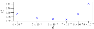
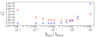
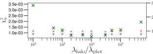
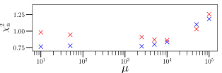
Figure 1: Parameters for the FOC equation. Top panel: photometric $\chi^{2}_{n}$ values versus $\epsilon$ (blue crosses). Second panel: $\chi^{2}_{n}$ versus $\lambda_{\rm kin}/\lambda_{\rm phot}$ (for $\lambda_{\rm phot}\,{\!=\!}\,1$) for the photometry (blue crosses) and the kinematics (red crosses). Third panel: $\chi^{2}_{n}$ versus $\lambda_{\rm kin}/\lambda_{\rm phot}$ (also where $\lambda_{\rm phot}\,{\!=\!}\,1$) for the dark matter density (green crosses). We also show the $\chi^{2}_{n}$ for the photometry (blue crosses) and the kinematics (red crosses) where the $\chi^{2}_{n}$ values are in reference to the right Y-axis numbers. Bottom panel: $\chi^{2}_{n}$ versus $\mu$ for the photometry (blue crosses) and the kinematics (red crosses).

The FOC parameters $\epsilon$, $\lambda_{k}$ and $\mu$ of equation 7 are chosen sequentially. We first fit only the photometry, leaving the parameters $\lambda_{1\dots 5}$ and $\mu$ fixed to zero and varying only $\epsilon$ (the parameter $\lambda_{k\,{\!=\!}\,0}$, or $\lambda_{\rm phot}$, normalises $\epsilon$ and for simplicity is set to $\lambda_{\rm phot}\,{\!=\!}\,1$). We measure the reduced chi-square (terms $\chi^{2}\,_{j}{}^{k}$ in equation 5), for the photometry ($k\,{\!=\!}\,0$) in the bulge region finding the relation between $\chi^{2}_{n}$ and $\epsilon$ shown in Figure 1 in the top panel. For too small $\epsilon$ the photometry does not have the power to change the model and so the $\chi^{2}_{n}$ is large. For too large $\epsilon$ the photometry has too much power, changing the particle weights too quickly compared to the orbital timescale, so that only the local observable (or pixel) that the particle is crossing is fitted. An optimum $\epsilon$ value allows the weight to change an averaged amount once it crosses all the observables that are along the particle’s orbit, so that its weights converge to a constant value. We find this optimum value at the minimum $\chi^{2}_{n}$, when $\epsilon\,{\!=\!}\,7.0\times 10^{-9}$.

Second, we find the best $\lambda_{k}$ for the IFU kinematic observables (where $k\,{\!=\!}\,1\dots 4$) defined also as $\lambda_{\rm kin}$. We use the previous best $\epsilon$ and fit the photometry together with the IFU kinematics for several values of $\lambda_{\rm kin}$. We measure both the photometric and kinematic reduced chi-square in the bulge region, obtaining the relations versus $\lambda_{\rm kin}$ shown in Figure 1 (second panel). The photometric $\chi^{2}_{n}$ has smaller values for small $\lambda_{\rm kin}$, and would be minimized for $\lambda_{\rm kin}\,{\!=\!}\,0$, because then only the photometry would be fitted without the additional kinematic constraints. As $\lambda_{\rm kin}$ increases, the kinematic observations have more power tailoring the model towards fitting the kinematics as well, as we see the kinematic $\chi^{2}_{n}$ decreasing for larger $\lambda_{\rm kin}$, which worsen the photometric $\chi^{2}_{n}$ if the kinematics get too much power. Similarly to $\epsilon$, if $\lambda_{\rm kin}$ increases too much, both the photometric and the kinematic $\chi^{2}_{n}$ get worse. We find an optimal value of $\lambda_{k}\,{\!=\!}\,2.5\times 10^{-1}$ for the minimum kinematic $\chi^{2}_{n}$ while the photometric $\chi^{2}_{n}$ is still small.

To find the best parameter $\lambda_{\rm halo}$ for the dark matter halo fitting, we fix the previously found parameters $\epsilon$ and $\lambda_{\rm kin}$and test different values of $\lambda_{\rm halo}$ versus the reduced chi-square of the dark matter halo density (Figure 1 third panel). We find the minimum $\chi^{2}_{n}$ at $\lambda_{\rm 6}\,{\!=\!}\,10^{4}$, where the photometric and the kinematic $\chi^{2}_{n}$ remain almost unchanged.

We determine the entropy magnitude term to be $\mu\,{\!=\!}\,5\times 10^{3}$ (Figure 1 bottom panel) in the same way, fixing the previous parameters and choosing the largest $\mu$ that still has small $\chi^{2}$ values for the photometry and the kinematics.

After setting the fitting parameters, we run M2M fits, showing an example in Figure 2 where the reduced chi-squares of the model observables from equation 5 are plotted versus time (iterations). In the phase $T_{\rm obs}$ the model temporal smoothed observables are calculated decreasing $\chi^{2}_{\rm n}$ at first and then staying constant. Then the fitting phase $T_{\rm M2M}$ starts where $\chi^{2}_{\rm n}$ of the photometry, kinematics and the dark matter halo decrease in time. Finally in the stability check phase $T_{\rm stab}$ the values of $\chi^{2}_{\rm n}$ increase slightly.

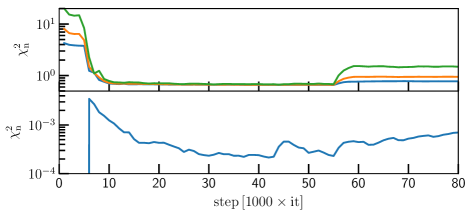
Figure 2: Reduced chi-square values as function of time for the M2M fitting of one model as defined in the main text. Top panel: photometry (blue), kinematics (green) and total (yellow) Bottom panel: dark matter halo density.

2.8 Exploring the effective potential parameters

B17 find good constraints for the mass ratio between the $\rm CB$ and the $\rm BPB$ while the dark matter distribution and the bar pattern speed are less constrained. Here, we use stellar kinematic and photometric observations as targets to better determine these properties. While the M2M method has the power to change the orbital distribution, thereby changing the model $\upsilon_{\rm los}$ $\sigma_{\rm los}$, $h3$, $h4$ and $L$ to match the observed kinematics, there are macroscopic potential parameters that limit the orbital phase space, and therefore a particular model will fit the data as well as these macroscopic parameters allow. Here we have three important dynamical quantities that are inputs to the M2M modelling and that impact the effective potential: the pattern speed of the bar ${\Omega_{\rm p}\,\,}$, the stellar mass-to-light ratio of the bulge in the 3.6${\rm\mu m}$ band ${\Upsilon_{3.6}\,\,}$ which, for a well fitted target observed luminosity, determines the total stellar mass in the bulge $M^{\rm B}_{\star}$, and the amount of dark matter in the bulge region ${M^{\rm B}_{\rm DM}\,\,}$. Therefore, we need to apply a method of meta-optimization where each M2M model is an optimisation itself that finds the orbit distribution that best matches the observations for fixed potential parameters. Then we vary ${\Omega_{\rm p}\,\,}$, ${\Upsilon_{3.6}\,\,}$ and ${M^{\rm B}_{\rm DM}\,\,}$ around reasonable values that we estimated from the literature, and then we find the range of values for which the M2M models overall best reproduce all sets of observations. To explore these three global parameters we create one cube (or grid) of model parameters for the Einasto dark matter profile, and a second cube for the NFW dark matter halo profile, where each model $\vec{\rm M}$ has the coordinates:

$$\vec{\rm M}=\left({\Upsilon_{3.6}\,\,},{M^{\rm B}_{\rm DM}\,\,},{\Omega_{\rm p}\,\,}\right)$$ (25)

For the Einasto cube we explore ${\Upsilon_{3.6}\,\,}$ in the range of $0.5-0.85\,{\rm M_{\odot}\,L_{\odot}^{-1}}$ in steps of $\Delta{\Upsilon_{3.6}\,\,}\,{\!=\!}\,0.05\,{\rm M_{\odot}\,L_{\odot}^{-1}}$ to produce a low resolution grid that allows us to quickly find the best fitting region, and then we include more values between $0.68-0.8\,{\rm M_{\odot}\,L_{\odot}^{-1}}$ in steps of $\Delta{\Upsilon_{3.6}\,\,}\,{\!=\!}\,0.02\,{\rm M_{\odot}\,L_{\odot}^{-1}}$. For ${M^{\rm B}_{\rm DM}\,\,}$ we explore $0.6-2.4\times 10^{10}\,{\rm M_{\odot}}$ in steps of $\Delta M_{\rm DM}\,{\!=\!}\,0.2\times 10^{10}\,{\rm M_{\odot}}$. For ${\Omega_{\rm p}\,\,}$ we explore the range $20-55\,{\rm km}\,{\rm s}^{\rm-1}\,{\rm kpc}^{-1}$ in steps of $\Delta{\Omega_{\rm p}\,\,}\,{\!=\!}\,5\,{\rm km}\,{\rm s}^{\rm-1}\,{\rm kpc}^{-1}$, building then a cube of parameters with $13({\Upsilon_{3.6}\,\,})\times 10({M^{\rm B}_{\rm DM}\,\,})\times 8({\Omega_{\rm p}\,\,})$, i.e., a total of 1040 M2M models with the Einasto dark matter profile.

For the NFW cube we explore ${\Upsilon_{3.6}\,\,}$ in the range $0.62-0.8\,{\rm M_{\odot}\,L_{\odot}^{-1}}$ in steps of $\Delta{\Upsilon_{3.6}\,\,}\,{\!=\!}\,0.02\,{\rm M_{\odot}\,L_{\odot}^{-1}}$. For ${M^{\rm B}_{\rm DM}\,\,}$ we explore $0.6-1.8\times 10^{10}\,{\rm M_{\odot}}$ in steps of $\Delta M_{\rm DM}\,{\!=\!}\,0.2\times 10^{10}\,{\rm M_{\odot}}$. For ${\Omega_{\rm p}\,\,}$ we explore $25-50\,{\rm km}\,{\rm s}^{\rm-1}\,{\rm kpc}^{-1}$ in steps of $\Delta{\Omega_{\rm p}\,\,}\,{\!=\!}\,5\,{\rm km}\,{\rm s}^{\rm-1}\,{\rm kpc}^{-1}$, giving a cube of parameters with $10({\Upsilon_{3.6}\,\,})\times 7({M^{\rm B}_{\rm DM}\,\,})\times 6({\Omega_{\rm p}\,\,})$, i.e., a total of 420 M2M models for the NFW cube.

Dark matter haloes are expected to be flattened in the central part of disc galaxies due to the influence of the disc gravitational potential. Widrow et al. (2003); Widrow & Dubinski (2005) explored different flattening values for the dark halo of M31, finding reasonable fits between $q\simeq 0.8$ and 1.0. Here we use a dark halo flattening of $q\,{\!=\!}\,0.85$ as our fiducial value for both dark matter density profiles, but we test the effects of different values on the final results. We explore $q\,{\!=\!}\,0.7$ and $q\,{\!=\!}\,1.0$, finding stellar mass distributions for the disc and the central region of the $\rm CB$ similar to the fiducial model. This is discussed further in Section 3.1.3.

2.9 Selection of best-matching models in effective potential parameter space

The selection of the best-matching models from the parameter grid just discussed cannot be done by straightforward $\chi^{2}$-minimization, because with the extended, high-quality data available here, systematic effects play a dominant role. These include uncertainties in the dust modelling, intrinsic asymmetries in the observed surface brightness distribution (Figure 17 in Section 3.2.2 below), uncertainties in the parametrisation of the dark matter density distribution, and likely gradients in ${\Upsilon_{3.6}\,\,}$ especially between the BPB and adjacent disk. Because of these systematic effects no model is found to give the best fit simultaneously in all regions of M31, and both photometric and kinematic observables.

In addition, while the M2M models are fitted to an impressive number of 224251 photometric and kinematic data values (pixels), the spatial distributions of photometric and kinematic pixels and their residuals $\Delta_{j}^{k}$ are substantially different. (i) Typical errors can differ between different variables, e.g., between $L$ and $\sigma_{\rm los}$, or $\sigma_{\rm los}$ and $h3$, leading to different ranges of $\Delta_{j}^{k}$; see Figure 3. (ii) For the same variable set, the errors depend on the spatial regions considered; e.g., relative photometric errors are smaller in the central bulge than in its outer parts or in the disc region (Figure 4 below). Yet in all of these locations the data may contain signatures important for specific physical properties of the system.

In consequence, combining all $(\Delta_{j}^{k})^{2}$ values linearly in one total $\chi^{2}_{\rm tot}$ and finding the M2M model with that minimum total chi-square will not adequately capture the entire structure of M31; e.g., it will lead to a model providing a good fit of the $\rm BPB$ region, but to an unsatisfactory fit in the smaller central $\rm CB$ region. In the following we therefore describe an alternative procedure which we believe leads to a more robust selection of the overall best-matching models for M31 given the available data.

Figure 3: Inverse relative errors of the photometric and the kinematic observations. The minimum and maximum errors are: $10^{2.76}$ and $10^{8.05}\,{\rm L_{\odot}}$ for the photometry, 0.1 and 15.5$\,{\rm km}\,{\rm s}^{\rm-1}$ for the velocity, 1.1 and 15.6$\,{\rm km}\,{\rm s}^{\rm-1}$ for the dispersion, $0.6\times 10^{-3}$ and $0.7\times 10^{-1}$ for $h3$ and $0.7\times 10^{-3}$ and $0.6\times 10^{-1}$ for $h4$. The median errors are $10^{4.67}\,{\rm L_{\odot}}$ for the photometry, 3.6$\,{\rm km}\,{\rm s}^{\rm-1}$ for the velocity, 3.8$\,{\rm km}\,{\rm s}^{\rm-1}$ for the dispersion, and 0.02 for $h3$ and $h4$.

2.9.1 Building a metric for the comparison with the observational data: five chi-square subsets

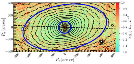
Figure 4: The M31 bulge surface luminosity relative error map. We define the region of the $\rm CB$ (CBR) within the blue circle, and the region of the $\rm BPB$ (BPR) is between the circle and the ellipse, and everything within the ellipse comprehend then the bulge region (BR). The surface-brightness isophotes in the 3.6${\rm\mu m}$ band are shown spaced with $\Delta\mu_{3.6}\,{\!=\!}\,0.25\,[{\rm mag}\,{\rm\,{\rm arcsec}^{-2}}]$. The value $\mu_{3.6}\,{\!=\!}\,16\,[{\rm mag}\,{\rm\,{\rm arcsec}^{-2}}]$ is shown with a dashed isophote and the disc major axis is at ${\rm PA}\,{\!=\!}\,38\degree$ (dash line). In white colour are the masked hot pixels and foreground stars.

Separating the observables $L$, $\upsilon_{\rm los}$, $\sigma_{\rm los}$, we first build five subsets of normalized $\chi^{2}$. These are motivated by the properties of the system that we are modelling, which is built from the three main substructures $\rm CB$, $\rm BPB$ and disc that we want to fit simultaneously well. The $\rm CB$ dominates the light in M31 within $R\lesssim 100\,{\rm arcsec}\,(380\,{\rm pc})$, defined as region CBR. Further out the $\rm BPB$ dominates the light within ellipses with semimajor axis $100\,{\rm arcsec}\!<\!R_{\rm mj}\!<\!700\,{\rm arcsec}$ (region BPR), and even further out the disc dominates (Beaton et al., 2007, B17); see Figure 4. We define five subsets of normalized $\chi^{2}$s:

• $\rm CB$ central photometry (${{\chi}^{2}}\,^{\rm CBR}_{\mu}$): we measure the normalized $\chi^{2}$ (per data point) of the photometry ($L_{3.6{\rm\mu m}}$) in the inner CBR within a diameter of 40$\,{\rm arcsec}$ (150$\,{\rm pc}$, $\sim R_{\rm e}/10$). With this we search for models that match the cuspy light profile in the centre of M31’s bulge.

• $\rm CB$ central dispersion (${{\chi}^{2}}\,^{\rm CBR}_{\sigma}$): the M31 dispersion profile shows two peaks of $\sigma_{\rm los}\,{\!\sim\!}\,170\,{\rm km}\,{\rm s}^{\rm-1}$ at $R\,{\!\sim\!}\,50\,{\rm arcsec}$, but drops to $\sigma_{\rm los}\,{\!\sim\!}\,150\,{\rm km}\,{\rm s}^{\rm-1}$ in the centre (Saglia et al., 2010; Opitsch et al., 2017). Therefore, we also measure the normalized $\chi^{2}$ of $\sigma_{\rm los}$ within $R_{\rm e}/10$, to find models of the grid that reproduce this feature.

• $\rm BPB$ photometry (${{\chi}^{2}}\,^{\rm BPR}_{\mu}$): we measure the normalized $\chi^{2}$ of the photometry in region BPR (Figure 4).

• $\rm BPB$ dispersion (${{\chi}^{2}}\,^{\rm BPR}_{\sigma}$): B17 show that the $\rm BPB$ and the $\rm CB$ of M31 have different kinematic properties. Hence, we calculate the normalized $\chi^{2}$ of the dispersion only in the BPR. This allows us also to find the dynamical mass within the bulge.

• $\rm BPB$ mean velocity (${{\chi}^{2}}\,^{\rm BPR}_{\upsilon}$): Tremaine & Weinberg (1984) showed that the bar pattern speed is related to the LOS velocity ($\upsilon_{\rm los}$) and the photometry. Therefore, we constrain the bar pattern speed with the normalized $\chi^{2}$ of the mean LOS velocity $\upsilon_{\rm los}$ in the bar region BPR.

In this way, each model $\vec{\rm M}$ is evaluated with five normalized $\chi^{2}$ parameters, $\vec{\chi}^{2}=\left({{\chi}^{2}}\,^{\rm CBR}_{\mu},{{\chi}^{2}}\,^{\rm CBR}_{\sigma},{{\chi}^{2}}\,^{\rm BPR}_{\mu},{{\chi}^{2}}\,^{\rm BPR}_{\sigma},{{\chi}^{2}}\,^{\rm BPR}_{\upsilon}\right)$. While the Gauss-Hermite coefficients $h3$ and $h4$ and all observables in the disc region are also fitted in each of the M2M models, we do not include $\chi^{2}$ subsets for them in the best model selection; later we show that the best models selected by the five subsets defined above satisfactory reproduce these observations as well.

2.9.2 Model ranking

Figure 5: Representation of the five chi-square subset volumes in the parameter space of ${\Upsilon_{3.6}\,\,}$, ${M^{\rm B}_{\rm DM}\,\,}$ and ${\Omega_{\rm p}\,\,}$. While the models have chi-square values in the whole cube, the coloured ellipses represent volumes where the chi-square values have the lowest values, showing ${\Delta\hat{\chi}^{2}}\,^{\rm CBR}_{\mu}$ (green), ${\Delta\hat{\chi}^{2}}\,^{\rm CBR}_{\sigma}$ (cyan), ${\Delta\hat{\chi}^{2}}\,^{\rm BPR}_{\mu}$ (blue), ${\Delta\hat{\chi}^{2}}\,^{\rm BPR}_{\sigma}$ (red) and ${\Delta\hat{\chi}^{2}}\,^{\rm BPR}_{\upsilon}$ (orange). The place where all ellipses intersect is where is located the overall best model $\vec{\rm M}_{\rm BM}$ (red circle). We also show the range of the acceptable models $\vec{\rm M}_{\rm AM}$ (green ring). The projections of the best model on each of the planes of the effective potential parameters are indicated with the dashed lines.

Table 1: Main parameters for the range of acceptable models for the Einasto dark dark matter profile $\vec{\rm M}_{\rm AM}^{\rm EIN}\,$; see text. The overall best matching model is Model JR804, corresponding to the best parameter values (B.V.). Inferred error ranges $\Delta^{+}_{-}$ are based on all acceptable models.

Model	${\Upsilon_{3.6}\,\,}$	${M^{\rm B}_{\rm DM}\,\,}$	${\Omega_{\rm p}\,\,}$	$M_{\star}^{\rm CB}$	$M_{\star}^{\rm BPB}$	$M_{\star}^{\rm B}$	$M_{\rm DM}^{\rm B(p)}$	$M_{\rm dyn}^{\rm B}$	${\Delta\hat{\chi}^{2}}\,^{\rm CBR}_{\mu}$	${\Delta\hat{\chi}^{2}}\,^{\rm CBR}_{\sigma}$	${\Delta\hat{\chi}^{2}}\,^{\rm BPR}_{\upsilon}$	${\Delta\hat{\chi}^{2}}\,^{\rm BPR}_{\mu}$	${\Delta\hat{\chi}^{2}}\,^{\rm BPR}_{\sigma}$	$\hat{\chi}^{2}_{\rm sum}$	$\Delta$$\hat{\chi}^{2}_{\rm sum}$
JR804	0.72	1.2	40	1.18	1.91	3.09	1.16	4.25	0.57	1.27	0.43	1.04	0.61	3.92	0.00
JR803	0.72	1.0	40	1.19	1.89	3.08	0.97	4.05	0.28	1.53	0.98	1.12	0.66	4.58	0.65
JR813	0.74	1.0	40	1.22	1.97	3.19	0.99	4.18	1.67	0.72	0.88	1.31	0.18	4.77	0.84
JR764	0.72	1.2	35	1.15	1.93	3.08	1.18	4.26	0.41	1.17	1.16	0.67	1.68	5.10	1.18
JR763	0.72	1.0	35	1.16	1.91	3.07	0.98	4.05	0.21	0.98	2.24	0.89	1.07	5.39	1.46
JR365	0.70	1.4	40	1.13	1.85	2.98	1.35	4.33	0.26	2.81	0.15	1.08	1.24	5.54	1.61
JR285	0.70	1.4	35	1.11	1.86	2.97	1.38	4.35	0.14	2.32	0.52	0.40	2.31	5.68	1.75
JR812	0.74	0.8	40	1.23	1.95	3.18	0.78	3.96	1.20	0.37	2.07	1.50	0.82	5.95	2.03
JR853	0.74	1.0	45	1.24	1.95	3.19	0.99	4.18	1.58	0.44	0.94	2.64	0.51	6.12	2.19
JR844	0.72	1.2	45	1.20	1.90	3.10	1.18	4.28	0.54	1.39	0.85	2.72	0.77	6.26	2.34
JR284	0.70	1.2	35	1.12	1.85	2.97	1.18	4.15	0.47	2.59	1.23	0.35	1.68	6.32	2.40
B.V.	0.72	1.2	40.0	1.18	1.91	3.09	1.16	4.25
$\Delta^{+}_{-}$	${}^{+0.02}_{-0.02}$	${}^{+0.2}_{-0.4}$	${}^{+5.0}_{-5.0}$	${}^{+0.06}_{-0.07}$	${}^{+0.06}_{-0.06}$	${}^{+0.10}_{-0.12}$	${}^{+0.22}_{-0.38}$	${}^{+0.10}_{-0.29}$

Notes: $M_{\star}^{\rm CB}$, $M_{\star}^{\rm BPB}$, ${M^{\rm B}_{\rm DM}\,\,}$, $M_{\rm DM}^{\rm B(p)}$ and $M_{\rm dyn}^{\rm B}$ in units of $10^{10}\,{\rm M_{\odot}}$. Parameters ${\Omega_{\rm p}\,\,}$ and ${\Upsilon_{3.6}\,\,}$ are in units of $\,{\rm km}\,{\rm s}^{\rm-1}\,{\rm kpc}^{-1}$ and $\,{\rm M_{\odot}\,L_{\odot}^{-1}}$ respectively.

Table 2: Main parameters of the range of acceptable models for the NFW dark matter profile $\vec{\rm M}_{\rm AM}^{\rm NFW}\,$. The overall best matching model is Model KR241, corresponding to the best parameter values (B.V.). Inferred error ranges $\Delta^{+}_{-}$ are based on all acceptable models with minimum given by the resolution of the model grid.

Model	${\Upsilon_{3.6}\,\,}$	${M^{\rm B}_{\rm DM}\,\,}$	${\Omega_{\rm p}\,\,}$	$M_{\star}^{\rm CB}$	$M_{\star}^{\rm BPB}$	$M_{\star}^{\rm B}$	$M_{\rm DM}^{\rm B(p)}$	$M_{\rm dyn}^{\rm B}$	${\Delta\hat{\chi}^{2}}\,^{\rm CBR}_{\mu}$	${\Delta\hat{\chi}^{2}}\,^{\rm CBR}_{\sigma}$	${\Delta\hat{\chi}^{2}}\,^{\rm BPR}_{\upsilon}$	${\Delta\hat{\chi}^{2}}\,^{\rm BPR}_{\mu}$	${\Delta\hat{\chi}^{2}}\,^{\rm BPR}_{\sigma}$	$\hat{\chi}^{2}_{\rm sum}$	$\Delta$$\hat{\chi}^{2}_{\rm sum}$
KR241	0.70	1.0	40	1.16	1.82	2.98	0.97	3.95	0.51	1.64	1.76	1.10	1.61	6.61	0.00
KR248	0.72	1.0	40	1.18	1.90	3.08	0.98	4.06	0.80	3.27	1.66	1.16	0.75	7.64	1.03
KR235	0.68	1.2	40	1.12	1.77	2.89	1.17	4.06	1.62	2.97	1.00	0.88	1.45	7.93	1.32
KR171	0.70	1.0	35	1.13	1.85	2.98	0.98	3.96	0.31	1.26	3.87	1.13	1.45	8.03	1.41
KR165	0.68	1.2	35	1.09	1.79	2.88	1.18	4.06	1.19	2.67	2.34	0.56	1.32	8.08	1.47
KR247	0.72	0.8	40	1.20	1.88	3.08	0.78	3.86	0.27	1.35	3.43	1.85	1.99	8.89	2.28
KR242	0.70	1.2	40	1.15	1.84	2.99	1.17	4.16	0.30	6.47	0.83	0.92	0.62	9.14	2.53
KR159	0.66	1.4	35	1.06	1.74	2.80	1.37	4.17	3.34	2.84	1.31	0.20	1.52	9.21	2.60
B.V.	0.70	1.0	40.0	1.16	1.82	2.98	0.97	3.95
$\Delta^{+}_{-}$	${}^{+0.02}_{-0.04}$	${}^{+0.4}_{-0.2}$	${}^{+5.0}_{-5.0}$	${}^{+0.04}_{-0.10}$	${}^{+0.08}_{-0.08}$	${}^{+0.10}_{-0.18}$	${}^{+0.40}_{-0.19}$	${}^{+0.22}_{-0.09}$

Notes: $M_{\star}^{\rm B}$, $M_{\star}^{\rm CB}$, $M_{\star}^{\rm BPB}$, ${M^{\rm B}_{\rm DM}\,\,}$, $M_{\rm DM}^{\rm B(p)}$ and $M_{\rm dyn}^{\rm B}$ in units of $10^{10}\,{\rm M_{\odot}}$. Parameters ${\Omega_{\rm p}\,\,}$ and ${\Upsilon_{3.6}\,\,}$ are in units of $\,{\rm km}\,{\rm s}^{\rm-1}\,{\rm kpc}^{-1}$ and $\,{\rm M_{\odot}\,L_{\odot}^{-1}}$ respectively.

In the space of the parameters ${\Upsilon_{3.6}\,\,}$, ${M^{\rm B}_{\rm DM}\,\,}$ and ${\Omega_{\rm p}\,\,}$, the normalized $\chi^{2}$ for each of the five subsets defines a region of acceptable models and a minimum $\chi^{2}$ model. However, we find that the subset chi-square values have stochastic local variations on top of the global trends, similarly as Morganti et al. (2013) found for their M2M models. Thus there may be several models that have $\chi^{2}$ values near the minimum. This stochasticity dominates the statistical uncertainty measured by normal delta chi-square analysis, which is not unexpected given the large amount of high quality data fitted and the remaining systematics.

Therefore, to better determine the global $\chi^{2}$ minimum in each subset, we follow Gebhardt et al. (2003) and obtain smoothed chi-square values for all models. Specifically, we average each model’s normalized chi-square with those of its $3\times 3\times 3-1\,{\!=\!}\,26$ neighbouring models (we also tested averaging with $3\times 2\,{\!=\!}\,6$ neighbouring models finding similar chi-square volumes and the same range of selected models). Then we find the minimum smoothed chi-square value ($\chi_{\rm min}^{2}$) in each of the subsets (which do not necessarily correspond to the same model $\vec{\rm M}$), obtaining for the Einasto halo grid

$${\vec{\chi}^{2}_{\rm min}} =\left({{\chi}^{2}}\,^{\rm CBR}_{\mu\,{\rm min}},{{\chi}^{2}}\,^{\rm CBR}_{\sigma\,{\rm min}},{{\chi}^{2}}\,^{\rm BPR}_{\mu\,{\rm min}},{{\chi}^{2}}\,^{\rm BPR}_{\sigma\,{\rm min}},{{\chi}^{2}}\,^{\rm BPR}_{\upsilon\,{\rm min}}\right)$$ (26)

$$=\left(0.195,0.267,0.774,2.717,3.544\right).$$ (27)

We also quantify the scatter introduced by the stochasticity described, calculating the standard deviation ($s$) of the original chi-square values of the models neighbouring the model with the minimum smoothed $\chi^{2}$ that is not on the border of the grid. For the five subsets we obtain ${s}\,^{\rm CBR}_{\mu}\,{\!=\!}\,0.062$, ${s}\,^{\rm CBR}_{\sigma}\,{\!=\!}\,0.155$, ${s}\,^{\rm BPR}_{\upsilon}\,{\!=\!}\,0.370$, ${s}\,^{\rm BPR}_{\mu}\,{\!=\!}\,0.040$ and ${s}\,^{\rm BPR}_{\sigma}\,{\!=\!}\,0.097$. Then we compute normalized $\Delta{\hat{\chi}}^{2}$ values for each model $\vec{\rm M}\left({\Upsilon_{3.6}\,\,},{M^{\rm B}_{\rm DM}\,\,},{\Omega_{\rm p}\,\,}\right)$ in all data subsets, ${\Delta\hat{\chi}^{2}}\,^{\rm CBR}_{\mu},{\Delta\hat{\chi}^{2}}\,^{\rm CBR}_{\sigma},{\Delta\hat{\chi}^{2}}\,^{\rm BPR}_{\mu},{\Delta\hat{\chi}^{2}}\,^{\rm BPR}_{\sigma},{\Delta\hat{\chi}^{2}}\,^{\rm BPR}_{\upsilon}$, where

$$\Delta{\hat{\chi}}^{2}\left({\rm subset}\right)=\left(\chi_{\rm n}^{2}\left({\rm subset}\right)-\chi^{2}_{\rm n\,min}\left({\rm subset}\right)\right)/s\left({\rm subset}\right)$$ (28)

based on the smoothed chi-squares and the standard deviation of the original chi-squares near minimum. In other words, we characterize the fit of a model to all the data in one of the five subsets by a single goodness-of-fit $\Delta{\hat{\chi}}^{2}$ parameter. This is the difference between the smoothed chi-square per data point relative to the minimum, normalized by the original scatter between neighbouring models around minimum. In this way, all the $\Delta{\hat{\chi}}^{2}$ are of similar magnitude, which allows us to compare models simultaneously with the signatures contained in the different data subsets.

The range of good models in each independent subset is defined by a volume in the space of ${\Upsilon_{3.6}\,\,}$, ${M^{\rm B}_{\rm DM}\,\,}$ and ${\Omega_{\rm p}\,\,}$, with values $\Delta{\hat{\chi}}^{2}\left({\rm subset}\right)\lesssim 1$, as illustrated in Figure 5. The volume where all subsets intersect with small chi-square values is where the models simultaneously have small deviations from the best model in all of the subsets, and corresponds to the region of the best-matching parameters ${\Upsilon_{3.6}\,\,}$, ${M^{\rm B}_{\rm DM}\,\,}$ and ${\Omega_{\rm p}\,\,}$.

We quantify the size of this region using a total delta chi-square $\Delta\hat{\chi}^{2}_{\rm sum}$ for each model, obtained by summing the normalized delta chi-square values for the $N_{\rm sub}\,{\!=\!}\,5$ subsets:

$$\Delta\hat{\chi}^{2}_{\rm sum}=\left(\hat{\chi}^{2}_{\rm sum}-\hat{\chi}^{2}_{\rm sum,min}\right);\qquad\hat{\chi}^{2}_{\rm sum}=\sum_{i}^{N_{\rm sub}}\Delta\hat{\chi}^{2}_{i}$$ (29)

where $\hat{\chi}^{2}_{\rm sum,min}$ is the minimum value of $\hat{\chi}^{2}_{\rm sum}$. $\Delta\hat{\chi}^{2}_{\rm sum}$ ranks the models from the best fitting model with minimum $\hat{\chi}^{2}_{\rm sum,min}\,{\!=\!}\,3.92$, up to the worst fitting model on the grid with $\hat{\chi}^{2}_{\rm sum}\,{\!=\!}\,954$. Sorting the models by $\hat{\chi}^{2}_{\rm sum}$ results in Table 1 for the Einasto grid, where we show just the range of acceptable models. The first model (JR804) is the overall best matching model $\vec{\rm M}_{\rm BM}$ and determines the best values of the parameters ${\Upsilon_{3.6}\,\,}$, ${M^{\rm B}_{\rm DM}\,\,}$and ${\Omega_{\rm p}\,\,}$. It does not necessarily has the minimum chi-square in each data subset, but achieves the best compromise in matching simultaneously all the observational datasets (see also Portail et al., 2017a).

Errors for parameters ${\Upsilon_{3.6}\,\,}$, ${M^{\rm B}_{\rm DM}\,\,}$and ${\Omega_{\rm p}\,\,}$are estimated from the maximum and minimum values in the acceptable models $\vec{\rm M}_{\rm AM}$ with

$$\vec{\rm M}_{\rm AM}= \left\{\forall\vec{\rm M}\,|\,\,\Delta\hat{\chi}^{2}_{\rm sum}\leq\delta\right\}$$ (30)

where we choose $\delta\,{\!=\!}\,2.7$, obtaining the range of models listed in Table 1. While the exact value of this threshold is arbitrary, inspection of the models within this limit shows that they reproduce all data satisfactorily including the most problematic outer bulge stellar kinematics. For $\delta\,{\!=\!}\,2.7$, no individual subset of any model has $\Delta\hat{\chi}^{2}_{i}>3$, while if we had chosen $\delta\,{\!=\!}\,1.3$, all subsets would be fitted with $\Delta\hat{\chi}^{2}_{i}<2$. These latter four models match the data even better, but we choose the more conservative $\Delta\,{\!=\!}\,2.7$ for the following reasons: (i) Compared to the number of models with $\Delta\hat{\chi}^{2}_{\rm sum}<2.7$, there is only a small number of models with $2.7<\Delta\hat{\chi}^{2}_{\rm sum}<4$, and these models allow only one new value of ${M^{\rm B}_{\rm DM}\,\,}$. (ii) At the same time, some individual subset $\Delta{\hat{\chi}}^{2}$ in this $2.7<\Delta\hat{\chi}^{2}_{\rm sum}<4$ range usually gets much worse, which is confirmed by inspecting the model fits. Thus we consider $\delta\,{\!=\!}\,2.7$ the most conservative choice consistent with the data. We note in passing that if the individual $\Delta\hat{\chi}^{2}_{i}$ were the square residual of single, Gaussian distributed measurements (which they are not), then $\Delta\hat{\chi}^{2}_{\rm sum}\,{\!=\!}\,2.7$ would correspond to 90 per cent of the $\chi^{2}$-distribution.

We also tested a different selection criterium to find the range of acceptable models. There we selected models for which each data subset has a maximum allowed deviation from the minimum in each subset, finding a similar range of models $\vec{\rm M}_{\rm AM}$ and consequently, a similar uncertainty range for the parameters ${\Upsilon_{3.6}\,\,}$, ${M^{\rm B}_{\rm DM}\,\,}$and ${\Omega_{\rm p}\,\,}$.

We finally applied the same procedure to the grid of NFW models (Table 2). The chi-square comparisons of the subset values and $\hat{\chi}^{2}_{\rm sum}$ between the Einasto and the NFW models indicate that the Einasto dark matter profile provides a better fit to the observations (the best NFW model KR241 has $\hat{\chi}^{2}_{\rm sum}=6.62$, already outside the range of acceptable models in the Einasto grid). Nonetheless, the range of parameters ${\Upsilon_{3.6}\,\,}$, ${M^{\rm B}_{\rm DM}\,\,}$and ${\Omega_{\rm p}\,\,}$obtained within the NFW models on their own is very similar to that found previously.

3 Results

Here we first describe the results of our parameter study for M31, and discuss the values we obtain for the mass-to-light ratio, dark matter mass in the bulge, and pattern speed, as well as the implied dark matter density and rotation curve decomposition (Section 3.1). In the second part (Section 3.2), we compare the photometric and kinematic maps and profiles of M31 with our best matching model.

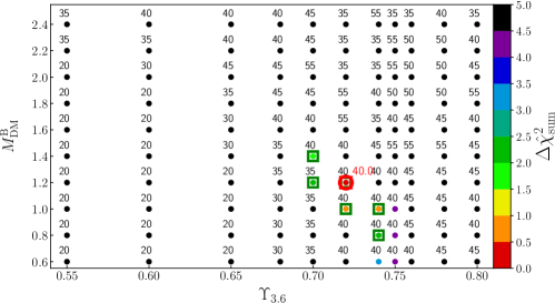
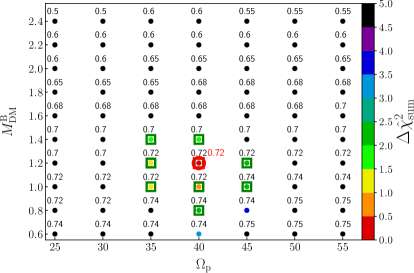
Figure 6: Range of acceptable models defined by the total goodness-of-fit $\Delta\hat{\chi}^{2}_{\rm sum}$, for an Einasto halo. The green squares mark the range of acceptable models, with the red circles marking the overall best matching model JR804. Left panel: $\Delta\hat{\chi}^{2}_{\rm sum}$ in the ${\Upsilon_{3.6}\,\,}$, ${M^{\rm B}_{\rm DM}\,\,}$plane, always selecting the minimum value along the parameter ${\Omega_{\rm p}\,\,}$axis. Right panel: $\Delta\hat{\chi}^{2}_{\rm sum}$ as function of ${\Omega_{\rm p}\,\,}$and ${M^{\rm B}_{\rm DM}\,\,}$, selecting the minimum value along the parameter ${\Upsilon_{3.6}\,\,}$axis. In black are shown models with $\Delta\hat{\chi}^{2}_{\rm sum}\geq 5$), with the largest value in the grid being $\hat{\chi}^{2}_{\rm sum}\,{\!=\!}\,954.7$.

3.1 M31 potential parameters from the best M2M models

From the model grid with Einasto dark matter halo profiles and the selection procedure explained in Section 2.9.2, we find the allowed range of values for the 3.6${\rm\mu m}$ mass-to-light ratio, the dark matter mass in the bulge, and pattern speed:

$${\Upsilon_{3.6}\!=\!0.72\!\pm\!0.02\,{\rm M_{\odot}\,L_{\odot}^{-1}}\,},$$ (31)

$${M^{\rm B}_{\rm DM}\!=\!1.2^{+0.2}_{-0.4}\times 10^{10}\,{\rm M_{\odot}}\,},$$ (32)

$${\Omega_{\rm p}\!=\!40\pm 5\,{\rm km}\,{\rm s}^{\rm-1}\,{\rm kpc}^{-1}}.$$ (33)

Models with an NFW halo fit the data significantly worse (Section 2.9.2), but result in similar parameter values: ${\Upsilon_{3.6}\!=\!0.70^{+0.02}_{-0.04}\,{\rm M_{\odot}\,L_{\odot}^{-1}}\,}$, ${M^{\rm B}_{\rm DM}\!=\!1.0^{+0.4}_{-0.2}\times 10^{10}\,{\rm M_{\odot}}\,}$, and ${\Omega_{\rm p}\!=\!40\!\pm\!5\,{\rm km}\,{\rm s}^{\rm-1}\,{\rm kpc}^{-1}}$. In both cases the central value is the best model and the errors are based on the range of acceptable models; see Table 1 (Einasto) and Table 2 (NFW). In the subsequent discussion we will therefore use the Einasto models.

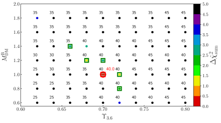
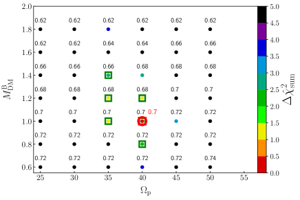
Figure 29: Range of acceptable models defined by the total goodness-of-fit $\Delta\hat{\chi}^{2}_{\rm sum}$, for an NFW halo. The green squares mark the range of acceptable models, with the red circles marking the overall best matching model KR241. Top panel: $\Delta\hat{\chi}^{2}_{\rm sum}$ in the ${\Upsilon_{3.6}\,\,}$, ${M^{\rm B}_{\rm DM}\,\,}$plane, always selecting the minimum value along the parameter ${\Omega_{\rm p}\,\,}$axis. Bottom panel: $\Delta\hat{\chi}^{2}_{\rm sum}$ as function of ${\Omega_{\rm p}\,\,}$and ${M^{\rm B}_{\rm DM}\,\,}$, selecting the minimum value along the parameter ${\Upsilon_{3.6}\,\,}$axis. In black are shown models with $\Delta\hat{\chi}^{2}_{\rm sum}\geq 5$).

Figure 6 shows the total goodness-of-fit $\Delta\hat{\chi}^{2}_{\rm sum}$ as function of the parameters ${\Upsilon_{3.6}\,\,}$, ${M^{\rm B}_{\rm DM}\,\,}$and ${\Omega_{\rm p}\,\,}$for the Einasto models. A small degeneracy between ${\Upsilon_{3.6}\,\,}$and ${M^{\rm B}_{\rm DM}\,\,}$remains within the range of allowed values. This is discussed further below. Figure 29 in the Appendix shows similar information for the NFW models, where the degeneracy is slightly increased because the more concentrated NFW profile has more mass within the bulge than the Einasto profile.

In the next subsections we explain how the physical parameters ${\Upsilon_{3.6}\,\,}$, ${M^{\rm B}_{\rm DM}\,\,}$and ${\Omega_{\rm p}\,\,}$are constrained by different subsets of the data. The corresponding signatures in the chi-square values between M31 data and models allow us to determine these parameters and, for example, break the degeneracy between the stellar mass and the dark matter mass in the bulge.

3.1.1 Constraining ${\Upsilon_{3.6}\,\,}$and ${M^{\rm B}_{\rm DM}\,\,}$

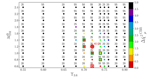
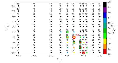
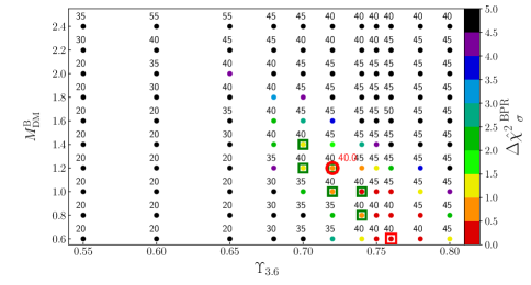
Figure 7: Breaking the degeneracy of ${\Upsilon_{3.6}\,\,}$and ${M^{\rm B}_{\rm DM}\,\,}$with different data sets. Plotted are the subset ${\Delta\hat{\chi}^{2}}\,^{\rm CBR}_{\mu}$ (top left), ${\Delta\hat{\chi}^{2}}\,^{\rm CBR}_{\sigma}$ (top right), ${\Delta\hat{\chi}^{2}}\,^{\rm BPR}_{\mu}$ (bottom left) and ${\Delta\hat{\chi}^{2}}\,^{\rm BPR}_{\sigma}$ (bottom right) for the Einasto models as function of the parameters ${\Upsilon_{3.6}\,\,}$ and ${M^{\rm B}_{\rm DM}\,\,}$, selecting for each pair of values the model with the minimum $\Delta\hat{\chi}^{2}_{i}$ along the ${\Omega_{\rm p}\,\,}$ axis. Numerical values for the points are given by the colour scale. The number next to each point corresponds to the ${\Omega_{\rm p}\,\,}$ value of the model with the lowest chi-square. We mark the best model JR804 (red circle), the models with the minimum values in each subset (red squares), and the range of acceptable models $\vec{\rm M}_{\rm AM}^{\rm EIN}\,$(green squares). The green squares do not necessarily have the pattern speed shown.

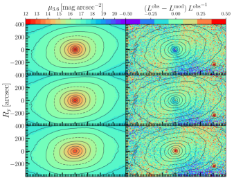
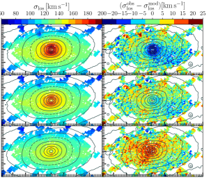
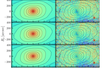
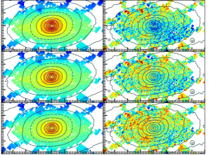
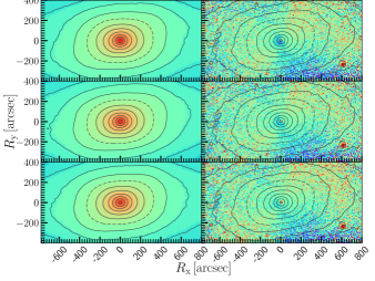
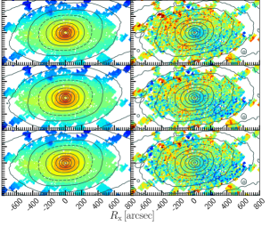
Figure 8: Model maps and their residuals with the observations for the surface-brightness (1st, 2nd columns) and the dispersion and residual (3rd and 4th columns). Case A with variation only in ${\Upsilon_{3.6}\,\,}$showing a model with ${\Upsilon_{3.6}\,\,}\,{\!=\!}\,0.80\,{\rm M_{\odot}\,L_{\odot}^{-1}}$ (1st row), the best model with ${\Upsilon_{3.6}\!=\!0.72\,{\rm M_{\odot}\,L_{\odot}^{-1}}\,}$(2nd row) and a model with ${\Upsilon_{3.6}\,\,}\,{\!=\!}\,0.65\,{\rm M_{\odot}\,L_{\odot}^{-1}}$ (3rd row). Case B with variation only in ${M^{\rm B}_{\rm DM}\,\,}$showing a model with ${M^{\rm B}_{\rm DM}\,\,}\,{\!=\!}\,1.6\!\times\!10^{10}\,{\rm M_{\odot}}$ (4th row), the best model with ${M^{\rm B}_{\rm DM}\!=\!1.2\times 10^{10}\,{\rm M_{\odot}}\,}$(5th row) and a model with ${M^{\rm B}_{\rm DM}\,\,}\,{\!=\!}\,0.8\!\times\!10^{10}\,{\rm M_{\odot}}$ (5th row). Case C (last three rows) with variation of ${\Upsilon_{3.6}\,\,}$and ${M^{\rm B}_{\rm DM}\,\,}$showing a model with ${\Upsilon_{3.6}\,\,}\,{\!=\!}\,0.75\,{\rm M_{\odot}\,L_{\odot}^{-1}}$ and ${M^{\rm B}_{\rm DM}\,\,}\,{\!=\!}\,0.8\!\times\!10^{10}\,{\rm M_{\odot}}$ (6th row), the best model (7th row), and a model with ${\Upsilon_{3.6}\,\,}\,{\!=\!}\,0.68\,{\rm M_{\odot}\,L_{\odot}^{-1}}$ and ${M^{\rm B}_{\rm DM}\,\,}\,{\!=\!}\,1.6\!\times\!10^{10}\,{\rm M_{\odot}}$ (8th row). We show the isophotes of the models (1st and 3rd column) and M31 (2nd and 4th column) spaced with $\Delta\mu_{3.6}\,{\!=\!}\,0.5\,[{\rm mag}\,{\rm\,{\rm arcsec}^{-2}}]$, with the $\mu_{3.6}\,{\!=\!}\,16\,[{\rm mag}\,{\rm\,{\rm arcsec}^{-2}}]$ ($I_{3.6}\,{\!=\!}\,3.4\!\times\!10^{3}\,\,{\rm L_{\odot}}\,\,{\rm pc}^{-2}$) isophote shown with a dashed contour.

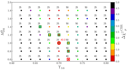
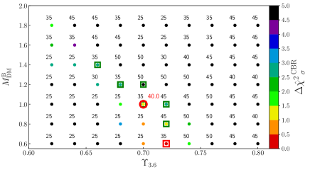
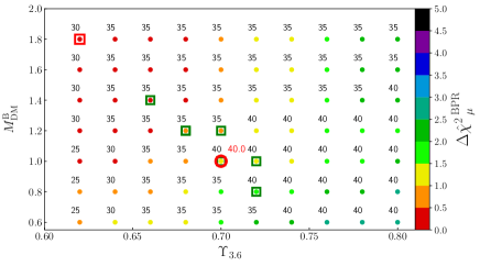
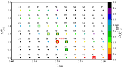
Figure 31: Results of the grid of models for the NFW dark matter halo for ${\Delta\hat{\chi}^{2}}\,^{\rm CBR}_{\mu}$, ${\Delta\hat{\chi}^{2}}\,^{\rm CBR}_{\sigma}$, ${\Delta\hat{\chi}^{2}}\,^{\rm BPR}_{\mu}$ and ${\Delta\hat{\chi}^{2}}\,^{\rm BPR}_{\sigma}$ as function of the parameters ${\Upsilon_{3.6}\,\,}$ and ${M^{\rm B}_{\rm DM}\,\,}$ selecting the lowest value along the axis of the parameter ${\Omega_{\rm p}\,\,}$. The values of each subset are he points that are coded in the coloured bar, and the number corresponds to the selected ${\Omega_{\rm p}\,\,}$. We mark the best model KR241 (red circle), the models with the minimum values in each subset (red squares), and the range of the acceptable models $\vec{\rm M}_{\rm AM}^{\rm NFW}\,$(green squares). The green squares do not necessarily agree with the pattern speed shown.

Figure 7 shows the separate goodness-of-fit values for the $\rm CB$ photometry and dispersion, ${\Delta\hat{\chi}^{2}}\,^{\rm CBR}_{\mu}$, ${\Delta\hat{\chi}^{2}}\,^{\rm CBR}_{\sigma}$, and for the $\rm BPB$ photometry and dispersion, ${\Delta\hat{\chi}^{2}}\,^{\rm BPR}_{\mu}$ and ${\Delta\hat{\chi}^{2}}\,^{\rm BPR}_{\sigma}$, as function of the stellar mass-to-light ratio and bulge dark matter mass in the Einasto models. For each ${\Upsilon_{3.6}\,\,}$and ${M^{\rm B}_{\rm DM}\,\,}$, we show the lowest $\Delta{\hat{\chi}}^{2}$ value along the ${\Omega_{\rm p}\,\,}$ axis. Equivalent results for the NFW model grid are shown in the appendix (Figure 31).

The $\rm CB$ region (CBR): we see from the top panels of Figure 7 that the parameter ${\Upsilon_{3.6}\,\,}$is strongly constrained by the dynamical properties of the $\rm CB$ in M31, where ${\Delta\hat{\chi}^{2}}\,^{\rm CBR}_{\mu}$ and ${\Delta\hat{\chi}^{2}}\,^{\rm CBR}_{\sigma}$ have very confined regions of low chi-square in ${\Upsilon_{3.6}\,\,}$. This is expected because in the very centre of the bulge the dynamics is governed mainly by potential of the stellar mass, which is set by ${\Upsilon_{3.6}\,\,}$, while the dark matter matters more in the outer part of the bulge, in the $\rm BPB$ region. The models that best match the photometry in the centre of the CBR (lowest ${\Delta\hat{\chi}^{2}}\,^{\rm CBR}_{\mu}$) are in the range ${\Upsilon_{3.6}\,\,}\,{\!=\!}\,0.70-0.74\,{\rm M_{\odot}\,L_{\odot}^{-1}}$, while the models that best match the central velocity dispersion in the CBR (lowest ${\Delta\hat{\chi}^{2}}\,^{\rm CBR}_{\sigma}$) are within ${\Upsilon_{3.6}\,\,}\,{\!=\!}\,0.70-0.75\,{\rm M_{\odot}\,L_{\odot}^{-1}}$. ${\Delta\hat{\chi}^{2}}\,^{\rm CBR}_{\mu}$ and ${\Delta\hat{\chi}^{2}}\,^{\rm CBR}_{\sigma}$ constrain the dark matter mass to be within ${M^{\rm B}_{\rm DM}\,\,}\!\leq\!1.4\times 10^{10}\,{\rm M_{\odot}}$, while the pattern speed has only a small effect in the CBR, which translates into having low values of ${\Delta\hat{\chi}^{2}}\,^{\rm CBR}_{\mu}$, ${\Delta\hat{\chi}^{2}}\,^{\rm CBR}_{\sigma}$ for a wide range of values of ${\Omega_{\rm p}\,\,}$.

The $\rm BPB$ region (BPR): the photometry in this region is less constraining with low values of ${\Delta\hat{\chi}^{2}}\,^{\rm BPR}_{\mu}$ over a wider range of ${\Upsilon_{3.6}\,\,}$and ${M^{\rm B}_{\rm DM}\,\,}$. This is because the stellar and dark matter can be exchanged to some degree and the M2M fitting can adjust rather well the stellar luminosity density within some range of values. Therefore, the acceptable models for ${\Delta\hat{\chi}^{2}}\,^{\rm BPR}_{\mu}$ are limited to ${\Upsilon_{3.6}\,\,}\!\lesssim\!0.74\,{\rm M_{\odot}\,L_{\odot}^{-1}}$ and ${M^{\rm B}_{\rm DM}\,\,}\!\gtrsim\!0.8\times 10^{10}\,{\rm M_{\odot}}$. The $\rm BPB$ velocity dispersion parameter ${\Delta\hat{\chi}^{2}}\,^{\rm BPR}_{\sigma}$ has a constrained region of low chi-square values in the range ${\Upsilon_{3.6}\,\,}\,{\!=\!}\,0.70-0.78\,{\rm M_{\odot}\,L_{\odot}^{-1}}$ and ${M^{\rm B}_{\rm DM}\,\,}\!\leq\!1.4\times 10^{10}\,{\rm M_{\odot}}$, so both $\rm BPB$ data sets together constrain ${M^{\rm B}_{\rm DM}\,\,}$. We show later in Figure 13 that the pattern speed is also constrained by ${\Delta\hat{\chi}^{2}}\,^{\rm BPR}_{\sigma}$. We note that, while the lowest chi-square values for each subset have slightly different locations in the space of ${\Upsilon_{3.6}\,\,}$and ${M^{\rm B}_{\rm DM}\,\,}$, the region of acceptable models overlap defining the range of best models, like our didactic Figure 5 illustrates.

The most important result shown by Figure 7 is that the degeneracy between the stellar mass-to-light ratio and the dark matter is broken by combining the different data subsets, particularly the $\rm CB$ photometry (${\Delta\hat{\chi}^{2}}\,^{\rm CBR}_{\mu}$) and dispersion (${\Delta\hat{\chi}^{2}}\,^{\rm CBR}_{\sigma}$) which are sensitive to ${\Upsilon_{3.6}\,\,}$and imply a tight range of values, which then narrow the bounds for the dark matter ${M^{\rm B}_{\rm DM}\,\,}$, strengthening the combined results from the $\rm BPB$ data (${\Delta\hat{\chi}^{2}}\,^{\rm BPR}_{\sigma}$ and ${\Delta\hat{\chi}^{2}}\,^{\rm BPR}_{\mu}$).

Figure 8 illustrates how ${\Upsilon_{3.6}\,\,}$and ${M^{\rm B}_{\rm DM}\,\,}$influence the velocity dispersion maps, and how the degeneracy between them is limited by the different data subsets. At lowest order, the mass in stars and dark matter can compensate. However, for given luminosity distribution and pattern speed, the gradient of the dispersion is changed with the steepness of the gravitational potential that depends on the stellar mass in the central bulge region and the dynamical mass in the outskirts of the bulge. Thus, for example, models that have too much dark matter mass within the bulge and low mass-to-light ratios result in a too flat dispersion profile.

Figure 8 shows photometric and kinematic maps of the best model ($\vec{\rm M}_{\rm BM}^{\rm EIN}$) and of models with modified values of ${\Upsilon_{3.6}\,\,}$and ${M^{\rm B}_{\rm DM}\,\,}$. Residual maps are also shown that illustrate how these physical parameters are connected with goodness-of-fit parameters ${\Delta\hat{\chi}^{2}}\,^{\rm CBR}_{\mu}$, ${\Delta\hat{\chi}^{2}}\,^{\rm CBR}_{\sigma}$, ${\Delta\hat{\chi}^{2}}\,^{\rm BPR}_{\mu}$ and ${\Delta\hat{\chi}^{2}}\,^{\rm BPR}_{\sigma}$. We consider three main cases: (A) variations of only the mass-to-light ratio ($\Delta{\Upsilon_{3.6}\,\,}$), (B) variations of only the dark matter mass in the bulge ($\Delta{M^{\rm B}_{\rm DM}\,\,}$), and (C) varying both simultaneously ($\Delta{\Upsilon_{3.6}\,\,}$, $\Delta{M^{\rm B}_{\rm DM}\,\,}$) showing how the degeneracy between these parameters is constrained:

(A) The top panels in Figure 8 show the best model compared to two models with the same dark matter mass and pattern speed, but with different mass-to-light ratios. The model with a larger ${\Upsilon_{3.6}\,\,}$ has a slightly worse fit to the photometry in the $\rm BPB$ region (BPR) (larger ${\Delta\hat{\chi}^{2}}\,^{\rm BPR}_{\mu}$), and a worse fit to the inner dispersion, which is higher in the model than in the data (larger ${\Delta\hat{\chi}^{2}}\,^{\rm BPR}_{\sigma}$). The high ${\Upsilon_{3.6}\,\,}$results in too much mass in the centre of the bulge, hence a too deep central potential, which has the consequence of a velocity dispersion that is higher than the observations. For the model with lower ${\Upsilon_{3.6}\,\,}$ (3rd row) the effects are the opposite. The most important result here is that the mass-to-light ratio has the strongest effect in the central region where the $\rm CB$ is, showing the important signature of the chi-square variables ${\Delta\hat{\chi}^{2}}\,^{\rm CBR}_{\mu}$ and ${\Delta\hat{\chi}^{2}}\,^{\rm CBR}_{\sigma}$.

(B) If we change only the dark matter mass within the bulge, we obtain similar effects on the velocity dispersion but on larger scales. The middle panels of Figure 8 show the best model and two models that have the same ${\Upsilon_{3.6}\,\,}$and ${\Omega_{\rm p}\,\,}$, but different ${M^{\rm B}_{\rm DM}\,\,}$. These two models overpredict (underpredict) the observed dispersion map outside the central bulge for too high (low) ${M^{\rm B}_{\rm DM}\,\,}$. In the $\rm BPB$ region the mass of the dark matter is comparable to the stellar bulge mass (typically 25 per cent of the stellar mass depending on the model), contributing significantly to the total dynamical mass, which is connected to the dispersion and is constrained by the data through the ${\Delta\hat{\chi}^{2}}\,^{\rm BPR}_{\mu}$ and ${\Delta\hat{\chi}^{2}}\,^{\rm BPR}_{\sigma}$ variables. Because the stellar mass is determined by ${\Upsilon_{3.6}\,\,}$ which is fixed by the central regions of the bulge, ${\Delta\hat{\chi}^{2}}\,^{\rm BPR}_{\mu}$ and ${\Delta\hat{\chi}^{2}}\,^{\rm BPR}_{\sigma}$ thus constrain the dark matter mass ${M^{\rm B}_{\rm DM}\,\,}$.

(C) Finally, considering the case of ${\Upsilon_{3.6}\,\,}$-${M^{\rm B}_{\rm DM}\,\,}$jointly: what happens if we decrease (increase) the mass-to-light ratio, but also increase (decrease) the dark matter mass content? Using our selection criteria in Section 2.9.2 we found a range of acceptable models around the best model parameters ${\Upsilon_{3.6}\!=\!0.72\!\pm\!0.02\,{\rm M_{\odot}\,L_{\odot}^{-1}}\,}$and ${M^{\rm B}_{\rm DM}\!=\!1.2^{+0.2}_{-0.4}\times 10^{10}\,{\rm M_{\odot}}\,}$, in the elongated region of Figure 6 (left panel). The stellar ${\Upsilon_{3.6}\,\,}$is constrained mostly by the data in the CBR, while the influence of the ${M^{\rm B}_{\rm DM}\,\,}$is strongest in the $\rm BPB$. Here we show two models just outside the range of acceptable models along this elongation. Therefore the differences between these models and the data are subtle, but they are still visible directly in the maps.

3.1.2 ${\Upsilon_{3.6}\,\,}$for the two bulge components

Table 3: Cases for different ${\Upsilon_{3.6}\,\,}$ values for the bulge components and the outer disc.

${\Upsilon_{3.6}\,\,}\,\,{\rm M_{\odot}\,L_{\odot}^{-1}}$	i)	ii)	iii)	iv)	v)	vi)
$\Upsilon^{\rm CB}$	0.72	0.72	0.72	0.72	0.72	0.72
$\Upsilon^{\rm BPB}$	0.70	0.68	0.72	0.72	0.72	0.72
$\Upsilon^{\rm d}$	0.70	0.68	0.55	0.65	0.80	0.85

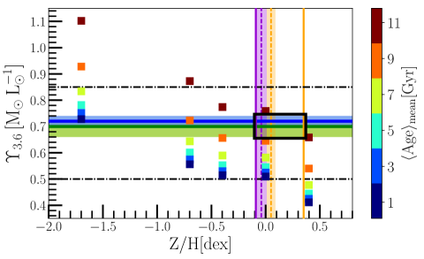
Figure 9: Stellar mass-to-light ratio in the 3.6${\rm\mu m}$ band as function of the metallicity. The best values are ${\Upsilon_{3.6}\!=\!0.72\!\pm\!0.02\,{\rm M_{\odot}\,L_{\odot}^{-1}}\,}$(blue line and shaded region) for the Einasto grid of models, and ${\Upsilon_{3.6}\!=\!0.70^{+0.02}_{-0.04}\,{\rm M_{\odot}\,L_{\odot}^{-1}}\,}$for the NFW grid (green line and shaded region), and the range of explored values of ${\Upsilon_{3.6}\,\,}$is shown with the dotted dashed horizontal lines. From Saglia et al. (2018) we show the $\,{\rm Z/H}$ of their model estimations (solid vertical lines), the average (vertical dashed line) and the root mean square (vertical shaded region) of the $\rm BPB$ (purple) and $\rm CB$ (orange). Meidt et al. (2014) estimate from stellar population evolution analysis predictions, relations for ${\Upsilon_{3.6}\,\,}$, the metallicity and the mean stellar age (squares). The black rectangle indicates the region of ${\Upsilon_{3.6}\,\,}$values that we expect to intersect with the values from the stellar populations analysis, given the metallicities estimated within M31’s bulge.

We find for the Einasto grid of models that the best range of values for the stellar mass-to-light ratio in the 3.6${\rm\mu m}$ band is ${\Upsilon_{3.6}\!=\!0.72\!\pm\!0.02\,{\rm M_{\odot}\,L_{\odot}^{-1}}\,}$. Given that the bulge of M31 has two components: a $\rm CB$ that likely formed very early from a hierarchical process, and a $\rm BPB$ formed by the redistribution of a disc component, we might expect different values of ${\Upsilon_{3.6}\,\,}$for each component. However, we now show that due to their measured metallicities and ages, their expected mass-to-light ratios in the 3.6${\rm\mu m}$ band are rather similar and that the best value represents well both bulge components.

In Figure 9 we show the stellar mass-to-light in the 3.6${\rm\mu m}$ band as function of metallicity and age computed by Meidt et al. (2014) using a stellar population analysis. These values assume a Chabrier initial mass function (IMF). Analysis of IMF sensitive absorption features in high signal-to-noise spectra by Zieleniewski et al. (2015) indicate that the IMF is consistent with Chabrier across the M31 bulge. We also over-plot in Figure 9 the ranges of metallicities within the bulge components of M31 measured by Saglia et al. (2018) (see also Opitsch, 2016) who find a $\rm CB$ with a metal rich and very old centre with an average of $\langle\,{\rm Z/H}\rangle^{\rm CB}\,{\!=\!}\,0.06\pm 0.05\,{\rm dex}$ (and as high as $\,{\rm Z/H}^{\rm CB}_{\rm model}\,{\!=\!}\,0.35\,{\rm dex}$) and ($12.9\pm 0.3\,{\rm Gyr}$); and a comparably old $\rm BPB$ ($12.8\pm 0.3\,{\rm Gyr}$) with a slightly sub-solar averaged metallicity of $\langle\,{\rm Z/H}\rangle^{\rm BPB}\,{\!=\!}\,-0.04\pm 0.01\,{\rm dex}$. Our range of best values for ${\Upsilon_{3.6}\,\,}$are in agreement with what is expected for stellar populations with these metallicities and average ages for a Chabrier IMF.

Note from Figure 9 that, in the 3.6${\rm\mu m}$ band, an old and slightly more metal-rich population could have a mass-to-light similar to that of a slightly younger and less metal-rich population, which is relevant given the negative metallicity gradient measured by Saglia et al. (2018) of $\nabla{\,{\rm Z/H}}^{\rm CB}\,{\!=\!}\,-0.5\pm 0.1\,{\rm dex}\,{\rm kpc}^{-1}$. This is not uncommon, as other classical bulges and elliptical galaxies show metallicity gradients with the most metal rich part in their centres (Koleva et al., 2011). The $\rm BPB$ is indeed slightly younger and less metal rich. Consequently, our assumption of a common value of ${\Upsilon_{3.6}\,\,}$ for both bulge components is not unexpected and is sufficient to reproduce the most important dynamical properties of the M31 bulge, while the narrow range of valid values suggests that any difference in mass-to-light between the two bulge components must be small. Saglia et al. (2018) also compute from stellar population analysis the expected V-band $\Upsilon$ for both bulge components, finding differences in mass-to-light by less than 10 per cent, reinforcing that our common mass-to-light is not unexpected.

However, in the outer disc region, beyond the bar, younger stars can decrease the mass-to-light ratio. Colour gradients also suggest a metallicity gradient between the more metal rich bulge and the outer disc (Courteau et al., 2011). To test these assumptions we also performed M2M fits with different ${\Upsilon_{3.6}\,\,}$values for the bulge components ($\Upsilon^{\rm CB},\,\Upsilon^{\rm BPB}$) and the disc ($\Upsilon^{\rm d}$), considering six cases shown in Table 3. We only find small changes in the dynamical properties of the model within the bulge region. As we show in the next section, even in the outer part of the disc ($R>10\,{\rm kpc}$) for lower ${\Upsilon_{3.6}\,\,}$in the outer disc we require small variations of $\,{\!\sim\!}\,$ 10 per cent of dark matter mass at that radius in order to match the H I rotation curve. These $\Upsilon^{\rm d}$ variations also encompass the changes which would be caused by the mass of the gas in the disc, which would increase the mass in the outer disc by less than 10 per cent.

3.1.3 Stellar and dark matter mass distribution

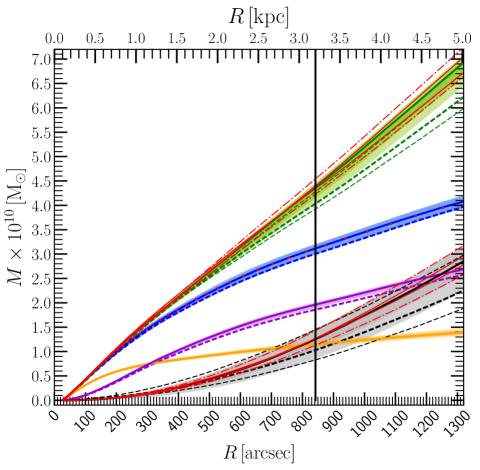
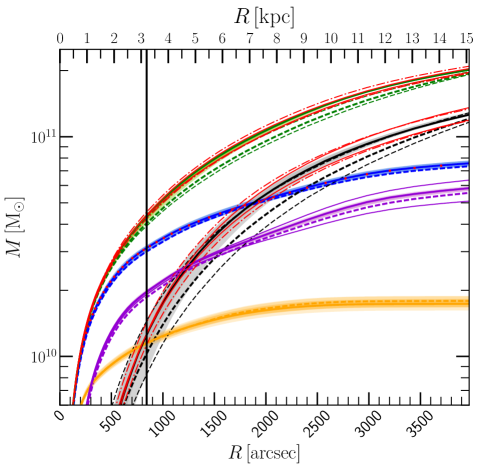
Figure 10: Cumulative mass profiles within 5$\,{\rm kpc}$ and (left panel) 15$\,{\rm kpc}$ (right panel) for the best model (JR804) of the grid with the Einasto dark matter profile (solid curves) and the best model (KR241) of the NFW grid (thick dashed curves), for the different components: $\rm CB$ (orange), $\rm BPB$ and disc (purple), total stellar (blue), dark matter (black) and dynamical mass (green). The range of acceptable models of the Einasto grid $\vec{\rm M}_{\rm AM}^{\rm EIN}\,$is shown in shaded regions. The most extreme values of ${M^{\rm B}_{\rm DM}\,\,}$profiles from the range of the models $\vec{\rm M}_{\rm AM}^{\rm NFW}\,$are shown with the thin dashed curves. The end of the de-projected $\rm BPB$ is at 3.2$\,{\rm kpc}$ (vertical black solid). We also show the $\rm BPB$ and disc cumulative mass profiles of the tests with $\Upsilon_{\rm d}\,{\!=\!}\,0.55\,{\rm M_{\odot}\,L_{\odot}^{-1}}$ and $0.85\,{\rm M_{\odot}\,L_{\odot}^{-1}}$ (lower and upper purple thin solid lines in right panel) (see cases iii and vi in Table 3) and the respective dark matter and dynamical mass profiles (upper and lower red solid curves). The tests for different flattening show masses within the bulge that lay within the range of models for $q\,{\!=\!}\,1.0$ and 0.7 (upper and lower red dot dash lines), and the stellar component in red dots. The profiles are function of the cylindrical radius $R$ summing the mass within a ellipsoidal volume with our fiducial flattening of $q\,{\!=\!}\,0.85$.

Figure 11: Azimuthally averaged circular velocity in the plane of the disc of the model JR804 (solid curves) and model KR241 (dashed curves) for the CB (orange), the $\rm BPB$ and the disc (purple), total stellar mass (blue curve), the dark matter (black curve), and the total circular velocity (green curve). The H I data of Corbelli et al. (2010) is shown out 15$\,{\rm kpc}$ (blue squares). The shaded regions correspond to the models with the Einasto profile $\vec{\rm M}_{\rm AM}^{\rm EIN}\,$. The dashed thin curves indicate the profiles of the models with the maximum and the minimum ${M^{\rm B}_{\rm DM}\,\,}$of the models $\vec{\rm M}_{\rm AM}^{\rm NFW}\,$. We show the circular velocity of the $\rm BPB$ and disc components of the tests with $\Upsilon_{\rm d}\,{\!=\!}\,0.55\,{\rm M_{\odot}\,L_{\odot}^{-1}}$ and $0.85\,{\rm M_{\odot}\,L_{\odot}^{-1}}$ (lower and upper thin purple solid curves) and corresponding dark matter halo circular velocities (upper and lower solid red curves), corresponding to cases iii and vi of Table 3. The test of the different flattening for $q\,{\!=\!}\,1.0$ (lower red dot dash line) and 0.7 (upper red dot dash line). The vertical black line marks the end of the $\rm BPB$.

In the previous section we found the range of 3.6${\rm\mu m}$ mass-to-light ratios and dark matter masses within the bulge that best reproduce the observations, thereby obtaining the range of stellar masses for each bulge component. Table 1 contains the resulting masses within 3.2$\,{\rm kpc}$ for the range of acceptable models with the Einasto dark matter haloes $\vec{\rm M}_{\rm AM}^{\rm EIN}\,$, with the best values being: $M_{\star}^{\rm CB}\,{\!=\!}\,1.18^{+0.06}_{-0.07}\times 10^{10}\,{\rm M_{\odot}}$ for the classical bulge, $M_{\star}^{\rm BPB}\,{\!=\!}\,1.91\pm 0.06\times 10^{10}\,{\rm M_{\odot}}$ for the $\rm BPB$, making a total bulge stellar mass of $M_{\star}^{\rm B}\,{\!=\!}\,3.09^{+0.10}_{-0.12}\times 10^{10}\,{\rm M_{\odot}}$. For the bulge dark matter mass we find ${M^{\rm B}_{\rm DM}\!=\!1.2^{+0.2}_{-0.4}\times 10^{10}\,{\rm M_{\odot}}\,}$finding then a total dynamical mass within the bulge of $M_{\rm dyn}^{\rm B}\,{\!=\!}\,4.25^{+0.10}_{-0.29}\times 10^{10}\,{\rm M_{\odot}}$. Integrating the mass of the $\rm CB$ out to 10$\,{\rm kpc}$ we obtain $M_{\star}^{\rm CB,10\,{\rm kpc}}\,{\!=\!}\,1.71^{+0.10}_{-0.09}\times 10^{10}\,{\rm M_{\odot}}$. Other bulge mass estimations in the literature neglect the composite nature of M31’s bulge, and therefore they recover similar values to our bulge total stellar mass ($M_{\star}^{\rm B}\,{\!=\!}\,4\times 10^{10}\,{\rm M_{\odot}}$; Kent, 1989), ($M_{\star}^{\rm B}\,{\!=\!}\,2.5\times 10^{10}\,{\rm M_{\odot}}$; Widrow et al., 2003). Our $\rm CB$ mass estimation is the lowest value in the literature for M31, which can be used to constrain the early formation history of M31.

The models with NFW haloes result in a similar range of values (Table 2), with $M_{\star}^{\rm CB}\,{\!=\!}\,1.16^{+0.04}_{-0.10}\times 10^{10}\,{\rm M_{\odot}}$ and $M_{\star}^{\rm BPB}\,{\!=\!}\,1.82\pm 0.08\times 10^{10}\,{\rm M_{\odot}}$, and a total stellar mass of $M_{\star}^{\rm B}\,{\!=\!}\,2.98^{+0.10}_{-0.18}\times 10^{10}\,{\rm M_{\odot}}$. The dark matter is ${M^{\rm B}_{\rm DM}\!=\!1.0^{+0.4}_{-0.2}\times 10^{10}\,{\rm M_{\odot}}\,}$with the total mass within the bulge being $M_{\rm dyn}^{\rm B}\,{\!=\!}\,3.95^{+0.22}_{-0.09}\times 10^{10}\,{\rm M_{\odot}}$.

In Figure 10 we present the cumulative mass profiles of the best models and the acceptable range models of the Einasto grid ($\vec{\rm M}_{\rm AM}^{\rm EIN}\,$) and the NFW grid ($\vec{\rm M}_{\rm AM}^{\rm NFW}\,$). The resulting range of models have very similar stellar mass profiles, and most of the total mass variation is due to the dark matter. The $\rm CB$ dominates the centre reaching the same mass of the $\rm BPB$ at 1.2$\,{\rm kpc}$ (300$\,{\rm arcsec}$). Further out the $\rm BPB$ dominates the stellar mass, and is almost double the mass of the $\rm CB$ at the end of the $\rm BPB$. Interestingly, the profiles show that the dark matter masses reach a similar value to the $\rm CB$ at end of the $\rm BPB$ at 3.2$\,{\rm kpc}$ (850$\,{\rm arcsec}$). The best values of the Einasto grid of models are similar within the errors to the best NFW models, with the best matching NFW models requiring slightly lower masses within 3.2$\,{\rm kpc}$. This is explained by the more cuspy density profile of the NFW profile: for the same mass at the end of the bulge (3.2$\,{\rm kpc}$) the NFW models have more dark matter distributed in the very centre than the Einasto models, as is shown by the density profiles in Figure 12.

We show in Figure 11 the circular velocity profiles of the models $\vec{\rm M}_{\rm BM}^{\rm EIN}$and $\vec{\rm M}_{\rm BM}^{\rm NFW}$within 15$\,{\rm kpc}$ $i.e.$ the radius where we fit the photometry. While the total dark matter within the bulge is fixed to a value ${M^{\rm B}_{\rm DM}\,\,}$during each M2M fit, where we select the values that best reproduce the photometry and the stellar kinematic observations, the dark matter in the disc region is determined during each run by fitting the H I rotation curve. We find that for the Einasto profile the range of dark matter masses and the resulting circular velocity values are more constrained than the range of values of the NFW profile.

We include in the mass profile and in the circular velocity figures variations of model JR804 with a flattening $q\,{\!=\!}\,0.7$ and 1.0, having dark matter mass and circular velocity values within the range of the acceptable models. As expected the dark matter mass profile deviates for different flattening values; however, the stellar mass profile remains within the range of the acceptable models. We also include in these figures tests with different ${\Upsilon_{3.6}\,\,}$values for the disc from Table 3, showing that even the extreme values $\Upsilon^{\rm d}\,{\!=\!}\,0.55\,{\rm M_{\odot}\,L_{\odot}^{-1}}$ and $\Upsilon^{\rm d}\,{\!=\!}\,0.85\,{\rm M_{\odot}\,L_{\odot}^{-1}}$ remain within the range of the acceptable models. The variation of the circular velocity in the disc region at $\,{\!\sim\!}\,$ 10$\,{\rm kpc}$ is small because most of the stellar mass is contained within this radius and the dark matter dominates at this distances, making the local variation of the stellar mass at $\,{\!\sim\!}\,$ 10$\,{\rm kpc}$ only a small contribution to the total circular velocity. We note that the tests of $\Upsilon^{\rm d}$ generate variations of stellar mass and surface mass density in the disc region that are larger than the mass contribution of the gas at this radius. Therefore, we do not need to include the gas contribution in the modelling.

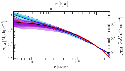
Figure 12: Dark matter density profiles of the best matching Einasto model (black curve) and the best NFW model (blue curve). The shaded regions correspond to the models with the Einasto profile $\vec{\rm M}_{\rm AM}^{\rm EIN}\,$(violet shade) and the NFW profile $\vec{\rm M}_{\rm AM}^{\rm NFW}\,$(cyan shade). The dotted blue dashed curve indicate the profile of the models with the maximum and the minimum ${M^{\rm B}_{\rm DM}\,\,}$of the models $\vec{\rm M}_{\rm AM}^{\rm NFW}\,$.

In Figure 12 we present the particle dark matter density profiles of the best models of the Einasto and the NFW grids, and the range of acceptable models. Fitting equation 22 to the density of the best Einasto model we recover the parameters $\rho_{\rm E}\,{\!=\!}\,1.29^{+0.12}_{-0.28}\times 10^{7}\,\,{\rm M_{\odot}}\,\,{\rm kpc}^{-3}$, $m_{\rm E}\,{\!=\!}\,7.8^{+1.1}_{-0.5}\,{\rm kpc}$ and $\alpha\,{\!=\!}\,0.51^{+0.22}_{-0.12}$ (or $n_{\rm Ein}\,{\!=\!}\,\alpha^{-1}\,{\!=\!}\,1.96\pm 0.6$), with errors from the range of best models. Similarly, a fit from equation 23 to the best NFW model, we recover the values $\rho_{\rm N}\,{\!=\!}\,1.54^{+1.9}_{-0.7}\times 10^{7}\,\,{\rm M_{\odot}}\,\,{\rm kpc}^{-3}$, and $m_{\rm N}\,{\!=\!}\,10.4^{+4.0}_{-3.4}\,{\rm kpc}$.

We find a dark matter mass of ${M^{\rm B}_{\rm DM}\!=\!1.2^{+0.2}_{-0.4}\times 10^{10}\,{\rm M_{\odot}}\,}$within 3.2$\,{\rm kpc}$ for the Einasto grid of models and ${M^{\rm B}_{\rm DM}\!=\!1.0^{+0.4}_{-0.2}\times 10^{10}\,{\rm M_{\odot}}\,}$for the NFW models, where the bulge stellar kinematics favours the cored Einasto profile. We find that the central dark matter masses are in agreement with cosmologically motivated haloes. Haloes with the virial mass M31 of $M_{{\rm DM}\,200}\,{\!=\!}\,1.04\times 10^{12}\,{\rm M_{\odot}}$ (Tamm et al., 2012) in cosmological simulations are expected to have an average concentration of $c_{200}\,{\!=\!}\,8.8$ and virial radius of $R_{200}\,{\!=\!}\,277\,{\rm kpc}$ (Correa et al., 2015a; Correa et al., 2015b, with Planck cosmology; Planck Collaboration et al. 2013). For such halo, the expected mass within 3.2$\,{\rm kpc}$ for a pure NFW halo is $M_{{\rm DM}\,200}^{3.2\,{\rm kpc}}\,{\!=\!}\,0.34\times 10^{10}\,{\rm M_{\odot}}$, lower than our measurement. However, the baryonic mass accretion can cause an adiabatic contraction of the halo that increases the central dark matter mass up to $M_{{\rm DM}\,200}^{3.2\,{\rm kpc}}\,{\!=\!}\,1.88\times 10^{10}\,{\rm M_{\odot}}$ in the most extreme case (Blumenthal et al., 1986), or a lower value of $M_{{\rm DM}\,200}^{3.2\,{\rm kpc}}\,{\!=\!}\,0.97\times 10^{10}\,{\rm M_{\odot}}$, as more recent hydrodynamical cosmological simulations show less contraction (Abadi et al., 2010, implemented with $\nu\,{\!=\!}\,0.4$ prescription from Dutton et al. 2011). Our results then agree with a moderate adiabatic contraction in the centre of the halo, but also favour a cored nature of the halo’s central distribution.

3.1.4 The box/peanut bulge and thin bar pattern speed (${\Omega_{\rm p}\,\,}$).

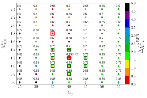
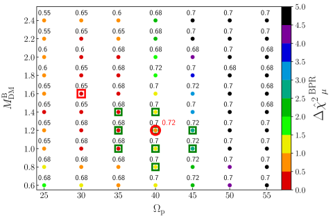
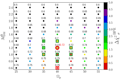
Figure 13: Results of the grid of models for the Einasto dark matter halo: ${\Delta\hat{\chi}^{2}}\,^{\rm BPR}_{\upsilon}$ (top), ${\Delta\hat{\chi}^{2}}\,^{\rm BPR}_{\mu}$ (middle) and ${\Delta\hat{\chi}^{2}}\,^{\rm BPR}_{\sigma}$ (bottom) as function of the parameters ${\Omega_{\rm p}\,\,}$ and ${M^{\rm B}_{\rm DM}\,\,}$, selecting the lowest value along the axis of the parameter ${\Upsilon_{3.6}\,\,}$. The values of each subset are the points that are coded in the coloured bar, and the number corresponds to the selected ${\Upsilon_{3.6}\,\,}$. We mark the best model JR804 (red circle), the models with the minimum values in each subset (red squares), and the range of acceptable models $\vec{\rm M}_{\rm AM}^{\rm EIN}\,$(green squares). The green squares do not necessarily agree with the shown ${\Upsilon_{3.6}\,\,}$.

The bar of M31 consists of a vertically thick structure that is the box/peanut bulge ($\rm BPB$) component, and the thin bar component that is mostly concentrated in the disc’s plane, where both structures are aligned and rotate at the same pattern speed. Most estimations of the M31 bar pattern speed are based on comparisons with gas kinematics, finding typically ${\Omega_{\rm p}\,\,}\!\!\!\!\approx\!\!50-60\,{\rm km}\,{\rm s}^{\rm-1}\,{\rm kpc}^{-1}$ (Stark & Binney, 1994; Berman, 2001; Berman & Loinard, 2002). Tremaine & Weinberg (1984) derived a relation from the continuity equation to determine the pattern speed of a two dimensional bar in disc galaxies directly from the observations using the information of the line-of-sight velocity ($\upsilon_{\rm los}$) and the photometry ($L_{3.6}$). Here we have the unique possibility to use new IFU stellar kinematics of the M31 bulge from O17 to determine the bar pattern speed. However, the disc inclination is too high to robustly determine it directly from the data using the Tremaine-Weinberg method. Therefore, we use this relation indirectly by comparing with models that have been fitted to the photometric and IFU observations, which have different pattern speed values. Then, we select the models with a good match of the velocity field in the bar region (${\Delta\hat{\chi}^{2}}\,^{\rm BPR}_{\upsilon}$), and the surface luminosity density (${\Delta\hat{\chi}^{2}}\,^{\rm BPR}_{\mu}$). Furthermore, the velocity dispersion ($\sigma_{\rm los}$) can also change the velocity through the total kinetic energy ($\sigma_{\rm los}^{2}+\upsilon_{\rm los}^{2}$), and therefore it also constrains the bar pattern speed. And so, combining these two variables with the variables ${\Delta\hat{\chi}^{2}}\,^{\rm CBR}_{\mu}$, ${\Delta\hat{\chi}^{2}}\,^{\rm CBR}_{\sigma}$ and ${\Delta\hat{\chi}^{2}}\,^{\rm BPR}_{\sigma}$ we are able to find the range of best matching models that also reproduce the velocity field in M31’s bulge. From the explored range of ${\Omega_{\rm p}\,\,}\,{\!=\!}\,20-55\,{\rm km}\,{\rm s}^{\rm-1}\,{\rm kpc}^{-1}$, we find ${\Omega_{\rm p}\,\,}\,{\!=\!}\,40\pm 5\,{\rm km}\,{\rm s}^{\rm-1}\,{\rm kpc}^{-1}$ for both grids of Einasto and NFW models (tables 1 and 2).

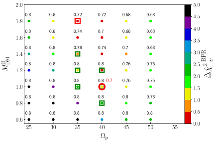
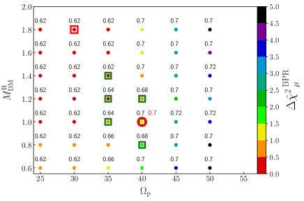
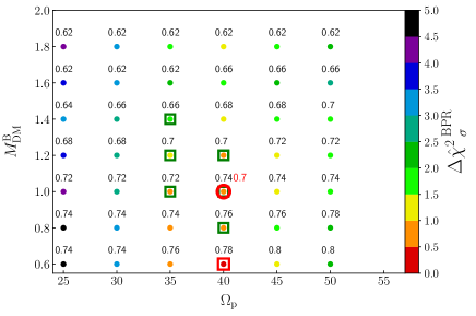
Figure 30: Results of the grid of models for the NFW dark matter halo for ${\Delta\hat{\chi}^{2}}\,^{\rm BPR}_{\upsilon}$, ${\Delta\hat{\chi}^{2}}\,^{\rm BPR}_{\mu}$ and ${\Delta\hat{\chi}^{2}}\,^{\rm BPR}_{\sigma}$ as function of the parameters ${\Omega_{\rm p}\,\,}$ and ${M^{\rm B}_{\rm DM}\,\,}$ selecting the lowest value along the axis of the parameter ${\Upsilon_{3.6}\,\,}$. The values of each subset are the points that are coded in the coloured bar, and the number corresponds to the selected ${\Upsilon_{3.6}\,\,}$. We mark the best model KR241 (red circle), the models with the minimum values in each subset (red squares), and the range of the acceptable models $\vec{\rm M}_{\rm AM}^{\rm NFW}\,$(green squares). The green squares do not necessarily agree with the shown ${\Upsilon_{3.6}\,\,}$.

In Figure 13 we show the results for ${\Delta\hat{\chi}^{2}}\,^{\rm BPR}_{\upsilon}$, ${\Delta\hat{\chi}^{2}}\,^{\rm BPR}_{\sigma}$, and ${\Delta\hat{\chi}^{2}}\,^{\rm BPR}_{\mu}$ as function of ${\Omega_{\rm p}\,\,}$and ${M^{\rm B}_{\rm DM}\,\,}$for the Einasto grid of models, with the best model located at ${M^{\rm B}_{\rm DM}\!=\!1.2\times 10^{10}\,{\rm M_{\odot}}\,}$and ${\Omega_{\rm p}\!=\!40\,{\rm km}\,{\rm s}^{\rm-1}\,{\rm kpc}^{-1}}$(NFW grid results in Figure 30). The variable ${\Delta\hat{\chi}^{2}}\,^{\rm BPR}_{\upsilon}$ has low values in the range of ${\Omega_{\rm p}\,\,}\,{\!=\!}\,30-45\,{\rm km}\,{\rm s}^{\rm-1}\,{\rm kpc}^{-1}$ and for ${M^{\rm B}_{\rm DM}\,\,}\geq 1.0\times 10^{10}\,{\rm M_{\odot}}$. ${\Delta\hat{\chi}^{2}}\,^{\rm BPR}_{\mu}$ has low values within ${\Omega_{\rm p}\,\,}\,{\!=\!}\,25-40\,{\rm km}\,{\rm s}^{\rm-1}\,{\rm kpc}^{-1}$ and within ${\Upsilon_{3.6}\,\,}\,{\!=\!}\,0.55-0.75\,{\rm M_{\odot}\,L_{\odot}^{-1}}$. The variable ${\Delta\hat{\chi}^{2}}\,^{\rm BPR}_{\sigma}$ has low values within ${\Omega_{\rm p}\,\,}\,{\!=\!}\,35-50\,{\rm km}\,{\rm s}^{\rm-1}\,{\rm kpc}^{-1}$ and ${M^{\rm B}_{\rm DM}\,\,}\leq 1.2\times 10^{10}\,{\rm M_{\odot}}$. Taking into account the restrictions given by the variables ${\Delta\hat{\chi}^{2}}\,^{\rm CBR}_{\mu}$, ${\Delta\hat{\chi}^{2}}\,^{\rm CBR}_{\sigma}$ and ${\Delta\hat{\chi}^{2}}\,^{\rm BPR}_{\sigma}$ that constrain the best values for the mass-to-light ratio and the dark matter mass to be ${\Upsilon_{3.6}\!=\!0.72\,{\rm M_{\odot}\,L_{\odot}^{-1}}\,}$and ${M^{\rm B}_{\rm DM}\!=\!1.2\times 10^{10}\,{\rm M_{\odot}}\,}$, we find that the best value for the bar pattern speed is ${\Omega_{\rm p}\!=\!40\,{\rm km}\,{\rm s}^{\rm-1}\,{\rm kpc}^{-1}}$.

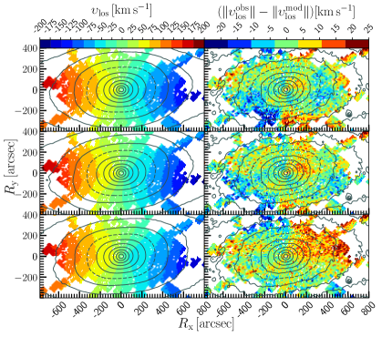
Figure 14: Model velocity maps (left column) and velocity residual with the observations (right column) for models with ${\Upsilon_{3.6}\,\,}\,{\!=\!}\,0.72\,{\rm M_{\odot}\,L_{\odot}^{-1}}$ and ${M^{\rm B}_{\rm DM}\,\,}\,{\!=\!}\,1.2\times 10^{10}\,{\rm M_{\odot}}$ with different pattern speeds, with 55 (top), 40 (middle) and 25$\,{\rm km}\,{\rm s}^{\rm-1}\,{\rm kpc}^{-1}$ (bottom). We show the isophotes of the models (first column) and M31 (second column) spaced with $\Delta\mu_{3.6}\,{\!=\!}\,0.5\,[{\rm mag}\,{\rm\,{\rm arcsec}^{-2}}]$ and the value $\mu_{3.6}\,{\!=\!}\,16\,[{\rm mag}\,{\rm\,{\rm arcsec}^{-2}}]$ is shown with a dashed isophote.

In order to show the effects of changing the bar pattern speed we present in Figure 14 the isophotes, the velocity maps and velocity residual maps of the best model ($\vec{\rm M}_{\rm BM}^{\rm EIN}$) and compare them with maps of two models with the same ${\Upsilon_{3.6}\,\,}$and ${M^{\rm B}_{\rm DM}\,\,}$, but with ${\Omega_{\rm p}\,\,}\,{\!=\!}\,25\,{\rm km}\,{\rm s}^{\rm-1}\,{\rm kpc}^{-1}$ and ${\Omega_{\rm p}\,\,}\,{\!=\!}\,55\,{\rm km}\,{\rm s}^{\rm-1}\,{\rm kpc}^{-1}$. The best model shows smaller residuals than the other two models. The isophotes slightly change in the outer parts of the $\rm BPB$ in response to the change of ${\Omega_{\rm p}\,\,}$, where the model with ${\Omega_{\rm p}\,\,}\,{\!=\!}\,25\,{\rm km}\,{\rm s}^{\rm-1}\,{\rm kpc}^{-1}$ shows slightly more boxy isophotes than the model with ${\Omega_{\rm p}\,\,}\,{\!=\!}\,55\,{\rm km}\,{\rm s}^{\rm-1}\,{\rm kpc}^{-1}$.

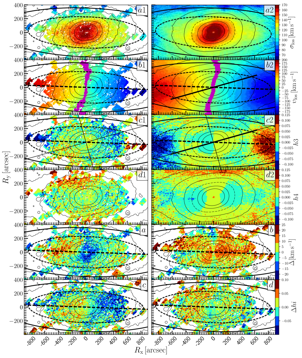
Figure 32: Surface-brightness isophotes and kinematic maps of M31 (left column) and a triaxial elliptical galaxy bulge model i.e. a model with the same parameters as model JR804, but with no pattern speed (${\Omega_{\rm p}\,\,}\,{\!=\!}\,0\,{\rm km}\,{\rm s}^{\rm-1}\,{\rm kpc}^{-1}$) (right column). Labels similar as Figure 23. The differences between the observations and the model are shown in panel ($a$) with $\Delta\,{\!=\!}\,\sigma_{\rm los}^{\rm obs}-\sigma_{\rm los}^{\rm model}$, ($b$) with $\Delta\,{\!=\!}\,||\upsilon_{\rm los}^{\rm obs}||-||\upsilon_{\rm los}^{\rm model}||$, ($c$) with $\Delta h3\,{\!=\!}\,h3^{\rm obs}-h3^{\rm model}$, and panel ($d$) with $\Delta h4\,{\!=\!}\,h4^{\rm obs}-h4^{\rm model}$.

Could the M31 bulge be a triaxial elliptical galaxy? Classical bulges are often considered to be akin to elliptical galaxies sitting in the centres of disc galaxies (Kormendy, 2013). Triaxial elliptical galaxies can also show rotation, but contrary to box/peanut bulges they show very little or no configuration rotation or no pattern speed. The historic consideration of the M31 bulge as a classical bulge implies that the bulge has no pattern speed. Many studies estimate the pattern speed of M31’s bulge (Stark & Binney, 1994; Berman, 2001; Berman & Loinard, 2002). The recent kinematic analysis of O17 (see their Section 5.3.) identify several signatures directly from the data, such as the bulge cylindrical rotation, which favours the barred nature of the M31 bulge over the triaxial elliptical galaxy bulge scenario. We compared our best matching model with the extreme cases of a model with a slowly rotating bar with ${\Omega_{\rm p}\,\,}\,{\!=\!}\,15\,{\rm km}\,{\rm s}^{\rm-1}\,{\rm kpc}^{-1}$ and another with ${\Omega_{\rm p}\,\,}\,{\!=\!}\,0\,{\rm km}\,{\rm s}^{\rm-1}\,{\rm kpc}^{-1}$, which is fundamentally a triaxial “elliptical” galaxy. In Figure 32 in the appendix we show the kinematic maps and residuals of the model with ${\Omega_{\rm p}\,\,}\,{\!=\!}\,0\,{\rm km}\,{\rm s}^{\rm-1}\,{\rm kpc}^{-1}$. The resulting models do indeed have a central triaxial bulge substructure; however, the fits are much worse in all the five subsets: the central stellar dispersion is higher than the observations, the dispersion plateaus reproduced by the best model are much weaker (see Section 3.2.4) and the stellar velocities are much lower. In addition, the fits to $h3$ and $h4$ are also worse, where the $h3-v_{\rm los}$ correlation observed in the bar region cannot be well reproduced. This test therefore demonstrates the barred nature of M31’s composite bulge.

3.1.5 The bar angle ($\theta_{\rm bar}$)

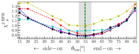
Figure 15: Variable ${{\chi}^{2}}\,^{\rm BPR}_{\mu}$ (chi-square of the photometry in the $\rm BPB$ region) for six different M2M models fitted with different bar angle values: the best model JR804 (black), model JR355 (red), model JR813 (magenta), model JR364 (blue), model JR683 (cyan) and model JR923 (yellow). Their properties are given in the main text. The fiducial value for our runs is $\theta_{\rm bar}\,{\!=\!}\,54\degree\!.7\pm 3\degree\!.8$ (vertical green line) from B17, which matches within errors with the minimum in all the tested models.

Here we show that the fiducial bar angle value chosen for the Einasto and NFW grid of models of $\theta_{\rm bar}\,{\!=\!}\,55\degree$ gives the best photometric fits in the $\rm BPB$ region compared to other values of $\theta_{\rm bar}$. In Figure 15 we show different values of the bar angle versus ${{\chi}^{2}}\,^{\rm BPR}_{\mu}$ for the best matching model JR804, confirming that our fiducial value $\theta_{\rm bar}\,{\!=\!}\,54\degree\!.7\pm 3\degree\!.8$ (Section 2.2) from B17 best matches the observations within the errors. The minimum value ${{\chi}^{2}}\,^{\rm BPR}_{\mu}$ depends on the bar angle to reproduce the observed twist of the bulge isophotes with respect to the projected major axis of the isophotes in the disk region, while the allowed range of angles is given by the flexibility of the made-to-measure technique to adapt the orbital distribution to match the twist. Furthermore, we have also considered models with very different dynamical properties such as model JR355 with $\left({\Upsilon_{3.6}\,\,},{M^{\rm B}_{\rm DM}\,\,},{\Omega_{\rm p}\,\,}\right)\,{\!=\!}\,\left(0.65,1.4,40\right)$, and models neighbouring the best model in variations of the mass-to-light ratio, such as JR813 with $\left({\Upsilon_{3.6}\,\,},{M^{\rm B}_{\rm DM}\,\,},{\Omega_{\rm p}\,\,}\right)\,{\!=\!}\,\left(0.70,1.0,40\right)$, JR364 with $\left({\Upsilon_{3.6}\,\,},{M^{\rm B}_{\rm DM}\,\,},{\Omega_{\rm p}\,\,}\right)\,{\!=\!}\,\left(0.74,1.0,40\right)$, and variations of the bar pattern speed, like JR683 with $\left({\Upsilon_{3.6}\,\,},{M^{\rm B}_{\rm DM}\,\,},{\Omega_{\rm p}\,\,}\right)\,{\!=\!}\,\left(0.72,1.0,25\right)$ and JR923 with $\left({\Upsilon_{3.6}\,\,},{M^{\rm B}_{\rm DM}\,\,},{\Omega_{\rm p}\,\,}\right)\,{\!=\!}\,\left(0.72,1.0,55\right)$, finding that these models also have a minimum values of ${{\chi}^{2}}\,^{\rm BPR}_{\mu}$ at $\theta_{\rm bar}\approx 55\degree$. This confirms that the fiducial bar angle value found by B17 is located in a global chi-square minimum, making unnecessary to vary the bar angle during our parameter search exploration.

3.2 Properties of the best M2M model

In the following section we compare the photometric and kinematic properties of M31 with the best model from the Einasto grid of models (JR804), showing the contribution of the $\rm CB$ and the $\rm BPB$ components separately as well. We find similar properties for the photometric and kinematic substructures in the best model of the grid with NFW haloes (KR241).

3.2.1 Surface-brightness maps

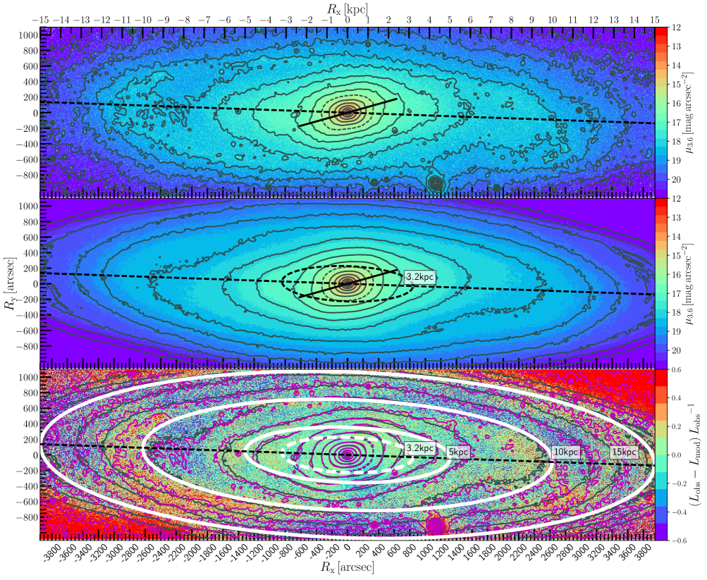
Figure 16: 3.6${\rm\mu m}$ band surface-brightness maps and isophotes spaced with $\Delta\mu_{3.6}\,{\!=\!}\,0.5\,[{\rm mag}\,{\rm\,{\rm arcsec}^{-2}}]$. The isophote with $\mu_{3.6}\,{\!=\!}\,16\,[{\rm mag}\,{\rm\,{\rm arcsec}^{-2}}]$ ($I_{3.6}\,{\!=\!}\,3.4\!\times\!10^{3}\,\,{\rm L_{\odot}}\,\,{\rm pc}^{-2}$) is shown with a dashed contour. Top panel: M31 with the disc projected major axis at ${\rm PA}_{\rm disc}\,{\!=\!}\,38\degree$ (dash line) and the projected bar major axis at ${\rm PA}_{\rm bar}\,{\!=\!}\,55\degree\!.7$ (solid line), where the de-projected thin bar semimajor axis $r_{\rm bar}^{\rm thin}\,{\!=\!}\,4.0\,{\rm kpc}\,\left(1000\,{\rm arcsec}\right)$ is in projection $R_{\rm bar}^{\rm thin}\,{\!=\!}\,2.3\,{\rm kpc}\,\left(600\,{\rm arcsec}\right)$ (B17). The north-east and the near side of the disc are in the top part of the panel (positive $R_{\rm y}$). Some foreground stars are visible as well as M32 in the bottom at $R_{\rm x}\,{\!\sim\!}\,1100\,{\rm arcsec}$. Middle panel: Model JR804 with the disc major axis (dash line) and bar major axis (solid line). We indicate the end of the $\rm BPB$ with a circle projected in the plane of the disk with $i\,{\!=\!}\,77\degree$ at the radii 3.2$\,{\rm kpc}$ (840$\,{\rm arcsec}$) (black ellipse). Bottom panel: fractional difference of the luminosity per pixel normalised by the observations. We also show the isophotes of M31 (magenta) and model JR804 (black). We show with circles projected into the disc the different substructures observed in M31 where the largest deviations occur, where the spiral arms are located 5$\,{\rm kpc}$ (1300$\,{\rm arcsec}$), the ring-like structures at 10$\,{\rm kpc}$ (2600$\,{\rm arcsec}$) and at 15$\,{\rm kpc}$ (3950$\,{\rm arcsec}$) (white ellipses). Note: model surface-brightness calculated from the temporal smoothed model observable $L$ with a pixel size of $8.63\,{\rm arcsec}$, as in the observations.

Figure 17: Bulge 3.6${\rm\mu m}$ band surface-brightness maps and isophotes spaced with $\Delta\mu_{3.6}\,{\!=\!}\,0.25\,[{\rm mag}\,{\rm\,{\rm arcsec}^{-2}}]$. The value $\mu_{3.6}\,{\!=\!}\,16\,[{\rm mag}\,{\rm\,{\rm arcsec}^{-2}}]$ ($I_{3.6}\,{\!=\!}\,3.4\!\times\!10^{3}\,\,{\rm L_{\odot}}\,\,{\rm pc}^{-2}$) is shown with a dashed isophote. Top panel: M31 with the disc projected major axis at ${\rm PA}\,{\!=\!}\,38\degree$ (dash line) and the projected bar major axis ${\rm PA}\,{\!=\!}\,55\degree\!.7$ (solid line), where the de-projected thin bar semimajor axis $r_{\rm bar}^{\rm thin}\,{\!=\!}\,4.0\,{\rm kpc}\,\left(1000\,{\rm arcsec}\right)$ is in projection $R_{\rm bar}^{\rm thin}\,{\!=\!}\,2.3\,{\rm kpc}\,\left(600\,{\rm arcsec}\right)$ (B17). The north-east and the near side of the disc are in the top part of the panel (positive $R_{\rm y}$). Middle panel: Model JR804 with the disc major axis (dash line) and the projected bar major axis (solid line). We indicate the end of the $\rm BPB$ with a circle projected in the plane of the disk with $i\,{\!=\!}\,77\degree$ at the radii 3.2$\,{\rm kpc}$ (840$\,{\rm arcsec}$) (black ellipse). Bottom panel: fractional difference of the luminosity per pixel normalised by the observations. We also show the isophotes of M31 (magenta) and the model (black). We show circles in the plane of the disk projected for $i\,{\!=\!}\,77\degree$ at radii 3.2kpc(840arcsec), 5kpc(1300arcsec) and 8kpc(2100arcsec) (white ellipses). Note: model surface-brightness calculated from the temporal smoothed model observable $L$ with a pixel size of $8.63\,{\rm arcsec}$, as in the observations.

We present our photometric M2M fitted map of the best model in Figure 16, compared to M31 in the 3.6${\rm\mu m}$ band, and a close-up of the bulge in Figure 17. The model fits in general well, particularly in the bulge. Note that because the model is a system in dynamical equilibrium and it has a symmetric structure (to 180°rotations) where the larger differences arise where substructures such as the spiral arms at $\,{\!\sim\!}\,5\,{\rm kpc}\,\left(1300\,{\rm arcsec}\right)$ and the ring at $\,{\!\sim\!}\,10\,{\rm kpc}\,\left(2600\,{\rm arcsec}\right)$ are found. Even the bulge region of M31 is not entirely symmetric, showing asymmetries between the near side (upper) of the bulge and the far side (bottom), where the near side has slightly higher luminosity than the far side, more noticeable for the isophotes with $\mu_{3.6}\geq 16\,{\rm mag\,{\rm arcsec^{-2}}}$. The dust extinction is too weak in the 3.6${\rm\mu m}$ band to cause this asymmetry, with typical V band extinction in the bulge of $A_{\rm V}\approx 1\,{\rm mag}$ (Draine et al., 2014) which corresponds to a 3.6${\rm\mu m}$ band extinction of $A_{3.6}\,{\!\sim\!}\,0.07\,{\rm mag}$ (Schlafly & Finkbeiner, 2011). Moreover, the expected dust extinction effect is the opposite of what is observed, where the luminosity on the far side should be systematically higher than in the near side, unlike the asymmetry observed in the map of Figure 17. The 3.6${\rm\mu m}$ photometric asymmetry also does not show a spatial correlation with high dust density regions (Figure 22) where the dust could have more emission. Another possibility is that the outer parts of the $\rm BPB$ are not in complete dynamical equilibrium, perhaps related to transient material in the disc, or even a possible passage of a satellite galaxy near its centre (Block et al., 2006; Dierickx et al., 2014; D’Souza & Bell, 2018).

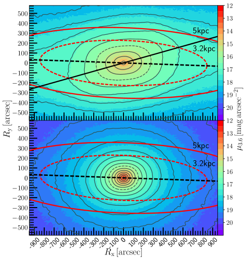
Figure 18: Surface-brightness maps of the $\rm BPB$ component (top panel) and the $\rm CB$ component (bottom panel). showing also their isophotes, spaced with $\Delta\mu_{3.6}\,{\!=\!}\,0.5\,[{\rm mag}\,{\rm\,{\rm arcsec}^{-2}}]$ and the value $\mu_{3.6}\,{\!=\!}\,16\,[{\rm mag}\,{\rm\,{\rm arcsec}^{-2}}]$ ($I_{3.6}\,{\!=\!}\,3.4\!\times\!10^{3}\,\,{\rm L_{\odot}}\,\,{\rm pc}^{-2}$) is shown with a dashed isophote. We show circles at radii 3.2 and 5$\,{\rm kpc}$ in the plane of the disk projected for an inclination of $i\,{\!=\!}\,77\degree$ (red ellipses). The projected bar major axis is shown at ${\rm PA}\,{\!=\!}\,55\degree\!.7$ (solid black line).

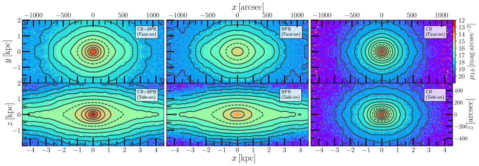
Figure 19: Different views of the best model bulge components. 3.6${\rm\mu m}$ band surface-brightness maps and isophotes spaced with $\Delta\mu_{3.6}\,{\!=\!}\,0.5\,[{\rm mag}\,{\rm\,{\rm arcsec}^{-2}}]$ and the value $\mu_{3.6}\,{\!=\!}\,16\,[{\rm mag}\,{\rm\,{\rm arcsec}^{-2}}]$ ($I_{3.6}\,{\!=\!}\,3.4\!\times\!10^{3}\,\,{\rm L_{\odot}}\,\,{\rm pc}^{-2}$) is shown with a dashed isophote. The orientations and bulge components are shown in the corners of each panel. Note: figures generated from the eight-folded model particles to decrease the noise.

In Figure 18 we show separately the $\rm CB$ component and the $\rm BPB$ component of model JR804. As we show with the surface-brightness profile in Section 3.2.2, the $\rm CB$ dominates in light and mass in the centre. Within $R\lesssim 100\,{\rm arcsec}$ it has roundish ellipses isophotes with their major axis roughly aligned with the disc major axis. The $\rm BPB$ is more extended and it has boxy isophotes that give to the combined bulge a twist of the isophotes as observed in M31, shifted away from the disc major axis by $\Delta{\rm PA}\,{\!\sim\!}\,13\degree$ (B17). The $\rm CB$ has a more oblate shape and therefore it cannot reproduce the triaxial structure and the twist. This is better revealed in Figure 19, where we show surface-brightness maps of the best model and its bulge components from different orientations.

3.2.2 Surface-brightness profiles

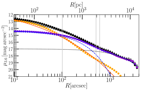
Figure 20: Azimuthally averaged surface-brightness profiles in the 3.6${\rm\mu m}$ band from ellipses fitted to the images of Figure 16 as function of the ellipse major axis for M31 (white triangles) and model JR804 (black circles) plotted out to 15$\,{\rm kpc}$. We also plot separately the $\rm CB$ component (orange circles) with its Sérsic fit (red curve) and the $\rm BPB$ and disc component (purple circles), with its Sérsic fit (dash blue curve), an exponential fit (black dotted curve), and the combined (solid blue curve). The vertical line at 100$\,{\rm arcsec}$ marks the end of region CBR. The vertical lines at 510$\,{\rm arcsec}$ and 600$\,{\rm arcsec}$ mark the end of the projected semimajor axis of the $\rm BPB$ and the thin bar (B17). Region BPR ends at 700$\,{\rm arcsec}$.

Table 4: Photometric profile fit parameters for the azimuthally averaged surface-brightness in the 3.6${\rm\mu m}$ band for M31 and the best model.

Parameter	M31	CB+BP+disc	BP+disc	CB
$n$	$2.58\!\pm\!0.04$	$2.24\!\pm\!0.04$	$1.10\!\pm\!0.01$	$4.3\!\pm\!0.2$
$\mu_{\rm e}$ [a]	$16.50\!\pm\!0.04$	$15.96\!\pm\!0.04$	$16.42\!\pm\!0.01$	$17.4\!\pm\!0.1$
$R_{\rm e}$ [$\,{\rm kpc}$ ]	$1.38\!\pm\!0.04$	$0.98\!\pm\!0.03$	$1.09\!\pm\!0.02$	$1.22\!\pm\!0.06$
$\epsilon_{R_{\rm e}}$	$0.37\!\pm\!0.01$	$0.33\!\pm\!0.01$	$0.40\!\pm\!0.01$	$0.25\!\pm\!0.02$
$\mu_{\rm o}$ [a]	$16.94\!\pm\!0.03$	$16.80\!\pm\!0.03$	$16.98\!\pm\!0.02$	-
$R_{\rm d}$ [$\,{\rm kpc}$ ]	$5.71\!\pm\!0.08$	$5.31\!\pm\!0.07$	$6.02\!\pm\!0.08$	-

Notes: parameters from top to bottom are the Séric profile parameters: index $n$, surface-brightness $\mu_{\rm e}$ in units of $\,{\rm mag\,{\rm arcsec^{-2}}}$, effective radius $R_{\rm e}$ and ellipticity $\epsilon_{R_{\rm e}}$; and the exponential profile parameters: the surface-brightness $\mu_{\rm o}$ in units of $\,{\rm mag\,{\rm arcsec^{-2}}}$ and the disc scale length $R_{\rm d}$. Each parameter error is calculated from the range of solutions taking 90 per cent of the chi-square distribution.

In Figure 20 we show the azimuthally averaged (AZAV) surface-brightness profiles of the best model and M31 in the 3.6${\rm\mu m}$ band calculated with ellipse-IRAF (Jedrzejewski, 1987) directly from the images shown in Figure 16. We also plot separately the $\rm BPB$ component and the $\rm CB$ component. We fit the total AZAV surface-brightness profiles of the best M2M model JR804 and M31 with a Sérsic profile (Sersic, 1968; Capaccioli, 1989) and an exponential profile out to 15$\,{\rm kpc}$ using a non-linear least squares (NLLS) minimization method, obtaining the parameters in Table 4. We also fit the model bulge components serparately, fitting the $\rm BPB$ and the disc with a Sérsic profile and an exponential profile; and the $\rm CB$ component alone with another Sérsic profile (Table 4).

We also use imfit (Erwin, 2015) to perform a 2D fit to the image of the $\rm CB$ component (Figure 18 bottom panel) with a Sérsic profile, finding values similar to the 1D fit, with $R^{\rm CB}_{\rm e}\,{\!=\!}\,273.3\,{\rm arcsec}$, $\mu^{\rm CB}_{\rm e}\,{\!=\!}\,17.1\,{\rm mag\,{\rm arcsec^{-2}}}$ and a Sérsic index of $n^{\rm CB}\,{\!=\!}\,3.4$. If we do not parameterise the contribution of the $\rm BPB$ in the fitting with an additional Sersic profile, the resulting Sérsic index from the usual photometric decomposition of one Sérsic profile and one exponential profile component is $n\approx 2$ as shown by Courteau et al. (2011) and also B17. Fisher & Drory (2008) show that the Sérsic index value of $n\,{\!\sim\!}\,2$ is a threshold that can distinguish galaxies with pseudobulges or classical bulges, the latter typically showing values larger than 2. However, in our scenario we have a composite bulge with a $\rm CB$ with a high Sérsic index $n^{\rm CB}\,{\!\sim\!}\,4$ and a $\rm BPB$ with a lower value $n^{\rm BPB}\,{\!\sim\!}\,1$, that when fitted with a single Sérsic and an exponential for the disc results in an intermediate value of 2.

The most important properties revealed in Figure 20 are:

1. The $\rm CB$ dominates in the central region $R\lesssim 100\,{\rm arcsec}$, and it is required in order to reproduce the central light concentration in M31, and, as we show later in more detail in Section 3.2.4, this component also reproduces the central dispersion profile observed in M31.

2. The $\rm BPB$ dominates in projection between $\,{\!\sim\!}\,100\,{\rm arcsec}$ and $R^{\rm BPB}\,{\!=\!}\,510\,{\rm arcsec}$; and the thin bar extends out to $R^{\rm thin}_{\rm bar}\,{\!=\!}\,600\,{\rm arcsec}$ (B17).

3. The surface-brightness bump at $R\,{\!\sim\!}\,1000$ $-$ $1300\,{\rm arcsec}$ $(4$ $-$ $5\,{\rm kpc})$ is caused by spiral arms and material trailing the bar (see Section 4.6.2 in B17), and it is reproduced in the M2M model by a slightly increase of the disc surface density.

4. The surface-brightness profile also reveals a second “bump” at 10$\,{\rm kpc}$ (Barmby et al., 2006; Courteau et al., 2011) from which point the surface brightness decreases at a faster rate. This is generally attributed to an additional contribution of the 10$\,{\rm kpc}$-ring structure, however it is also possible to attribute this to a change in the SB profile. M31 is a barred galaxy, which are systems that often develop such a break due to the secular evolution of the disc due to the angular momentum transfer with the bar through the Lindblad resonances, and also due to the redistribution of the disc material by the bar formation (Debattista et al., 2006). As we show later, in Section 3.2.5, we find that the outer Lindblad resonance is indeed located at $11\pm 1\,{\rm kpc}$, supporting this scenario. This indicates that the disc of M31 could be a mild Type II.o-OLR disc, with of a SB break at $\,{\!\sim\!}\,10\,{\rm kpc}$ related to a ring-like structure near the OLR resonance (Erwin et al., 2008; Kim et al., 2014), like the galaxy NGC3504, but more difficult to detect due to the high disc inclination. This would imply that a broken profile would be better suited for the photometric parametrisation of the outer M31 stellar disc, rather than the standard single exponential profile.

3.2.3 Dust extinction effects on the observed kinematics

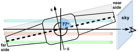
Figure 21: Diagram of M31 asymmetric projection effects due to the dust and the geometrical orientation with a disc inclination $i\,{\!=\!}\,77\degree$. Without extinction M31 projects into an image where the near and the far side are symmetric to the observer (right). However, if the light has a strong extinction by the dust located in the plane of the disc (dashed line) the observer detects an asymmetry. With strong extinction the light integrated along the near side of the disc (blue upper tube) will be dominated by the outer and younger part of the disk, while the material within the dashed area will be obscured by the dust in the plane of the disc. The opposite occurs in the far side of the disk, where the inner part of the disc dominates (green bottom tube). The bulge also projects asymmetrically and as a consequence the region where most of the light of the bulge is detected is slightly shifted to the far side (bottom) from the bulge centre (red middle tube), being then the deepest part of the bulge.

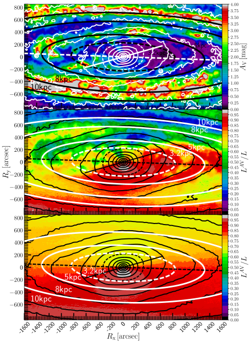
Figure 22: Top panel: M31 absorption map in the V band calculated from equation 13 and the dust surface mass map (Draine et al., 2014), with overplotted white isophotes of the M31’s 3.6${\rm\mu m}$ band image. Middle panel: $L^{A{\rm V}}\,L^{-1}$ map of model JR804 with overplotted model black isophotes in the 3.6${\rm\mu m}$ band. Note the light grey region near the bulge centre where the effects of the extinction in the V band are minimal. Bottom pane: $L^{A{\rm V}}\,L^{-1}$ map and 3.6${\rm\mu m}$ band isophotes for a model with the parameters of JR804, but observed and fitted through a dust map with a constant absorption of $A_{\rm V}\,{\!=\!}\,0.5\,{\rm mag}$. All panels: the disc projected major axis is shown with a dash line, with the near side of the disc in the upper part of the figures (positive $R_{\rm y}$), and the projected bar major axis is shown with a solid line. We show circles at the radii 3.2, 5, 8 and 10$\,{\rm kpc}$ in the plane of the disk projected for $i\,{\!=\!}\,77\degree$ (white and black ellipses). The isophotes are spaced with $\Delta\mu_{3.6}\,{\!=\!}\,0.5\,[{\rm mag}\,{\rm\,{\rm arcsec}^{-2}}]$ and $\mu_{3.6}\,{\!=\!}\,16\,[{\rm mag}\,{\rm\,{\rm arcsec}^{-2}}]$ is shown with a dashed isophote.

Given that the IFU M31 bulge stellar kinematic observations (O17) are in the V band, we have included the effects of the dust extinction in our modelling implemented according to Section 2.3.4. The diagram in Figure 21 qualitatively shows that, when some of the light of the galaxy is absorbed by the dust located in the plane of the disc, the projected image can have asymmetries between the near side of the disc and the far side. These asymmetries are strongly reflected in the stellar kinematics, as we show in the following sections. The line-of-sight to the far side of the disc penetrates more deeply into the galaxy than the near side. Thus, for example, the deepest region in the bulge is located slightly towards the far side from the bulge centre. A similar effect has also been detected in the reddening of RGB stars in M31’s disk (Dalcanton et al., 2015).

As the dust effects in the 3.6${\rm\mu m}$ band are very weak, we observe the model without dust extinction to fit the light in this band, which corresponds to the model light observable $L$. We also observe the model through the V band extinction map shown in Figure 22 (top panel), which results in the model observable $L^{A{\rm V}}$. In Figure 22 (middle panel) we show a map of the fraction of the absorbed and non absorbed light of the model ($L^{A{\rm V}}\,L^{-1}$). Without dust the near and the far side of the disc are symmetric, as in Figure 17 (middle panel); however with dust extinction the model produces asymmetries between both sides, as shown in Figure 22 (middle panel). The regions of the map with a ratio of $L^{A{\rm V}}\,L^{-1}\,{\!=\!}\,1$ are where all the light is detected, while for a ratio of zero the light is completely absorbed. Note that the ratio $L^{A{\rm V}}\,L^{-1}$ is proportional to the ratio between the light in the V band and the 3.6${\rm\mu m}$ band.

The map in Figure 22 (middle panel) reveals interesting features that are caused not only by the dust absorption itself, but also by the geometrical orientation of M31 with its disc inclination $i\,{\!=\!}\,77\degree$ and its bar angle $\theta_{\rm bar}\,{\!=\!}\,54\degree\!.7$. The least absorbed (or deepest) region in the M31 bulge is shifted from the centre to the far side of the disc (light grey region at $R_{y}\,{\!\sim\!}\,-100\,{\rm arcsec}$), as expected from the diagram in Figure 21, and the most extreme effect of extinction near the M31 bulge is in the near side of the disc, between $R_{\rm y}\,{\!\sim\!}\,200\,{\rm arcsec}$ and 400$\,{\rm arcsec}$ (green and blue regions), which are produced by the dust accumulated in the spiral arms. In addition, regions with large amounts of dust, but at the far side of the disc, can have weak effects on the light extinction like, for example, the far side at $R_{\rm y}\,{\!\sim\!}\,-500\,{\rm arcsec}$ where the outer ring is with a large dust lane.

In the bottom panel of Figure 22 we show a fit where we used a constant light absorption of $A_{\rm V}\,{\!=\!}\,0.5\,{\rm mag}$ to estimate how the heterogeneity of the M31 dust map (Draine et al., 2014) affects the ratio $L^{A{\rm V}}\,L^{-1}$, finding that the general features and the asymmetry are also reproduced. Dalcanton et al. (2015) finds lower absorption values in M31 than Draine et al. (2014); and so to investigate this we reduced the absorption values of the dust map by 50 per cent. We found a model with properties similar to the overall best model that again produced the observed asymmetries, but weaker than the fiducial model.

We conclude that the most important consequence of the dust extinction for the kinematics in the V band is that kinematic asymmetries are generated between the near side of the disc and the far side, because the light integrated along the line-of-sight can be dominated by different structures with different intrinsic kinematic properties. An example of this is shown by Baes & Dejonghe (1999) for elliptical galaxies. Furthermore, it is important to consider that neither the near side of the disc, nor the far side, have the complete signature along the line of sight, although the far side is much less affected by light extinction.

3.2.4 Stellar kinematics

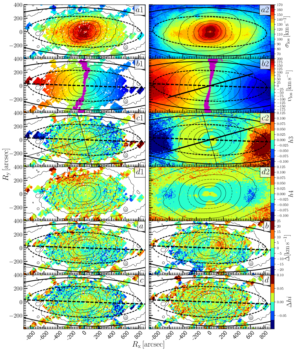
Figure 23: Isophotes and kinematic maps of $\sigma_{\rm los}$, $\upsilon_{\rm los}$, $h3$, $h4$ of M31 (O17) ($a1$, $b1$, $c1$, $d1$) and model JR804 (panels $a2$, $b2$, $c2$, $d2$), showing isophotes spaced every $\Delta\mu_{3.6}\,{\!=\!}\,0.5\,[{\rm mag}\,{\rm\,{\rm arcsec}^{-2}}]$ and $\mu_{3.6}\,{\!=\!}\,16\,[{\rm mag}\,{\rm\,{\rm arcsec}^{-2}}]$ in dashed isophote. We exclude the central isophotes to better reveal the kinematic features. Some panels display two circles projected on the disc’s plane with $i\,{\!=\!}\,77\degree$ at 3.2$\,{\rm kpc}$ (black dashed ellipse) and 8$\,{\rm kpc}$ (solid black ellipse), the projected disk major axis (dash black line at ${\rm PA}\,{\!=\!}\,38\degree$), and the projected bar major axis (black line at ${\rm PA}\,{\!=\!}\,55\degree\!.7$) and minor axis (black line at ${\rm PA}\,{\!=\!}\,145\degree\!.7$). The thick black lines in panels ($b2$, $c2$) mark the projected thin bar major axis, where the de-projected semimajor axis $r_{\rm bar}^{\rm thin}\,{\!=\!}\,4.0\,{\rm kpc}\,\left(1000\,{\rm arcsec}\right)$ is in projection $R_{\rm bar}^{\rm thin}\,{\!=\!}\,2.3\,{\rm kpc}\,\left(600\,{\rm arcsec}\right)$ (B17). The differences between the observations and the model are shown in panel ($a$) with $\Delta\,{\!=\!}\,\sigma_{\rm los}^{\rm obs}-\sigma_{\rm los}^{\rm model}$, ($b$) with $\Delta\,{\!=\!}\,||\upsilon_{\rm los}^{\rm obs}||-||\upsilon_{\rm los}^{\rm model}||$, ($c$) with $\Delta h3\,{\!=\!}\,h3^{\rm obs}-h3^{\rm model}$, and panel ($d$) with $\Delta h4\,{\!=\!}\,h4^{\rm obs}-h4^{\rm model}$. We show the zero velocity values within a range $\upsilon_{\rm los}\,{\!=\!}\,0\pm 5\,{\rm km}\,{\rm s}^{\rm-1}$ (magenta) in panels $b1$ and $b2$.

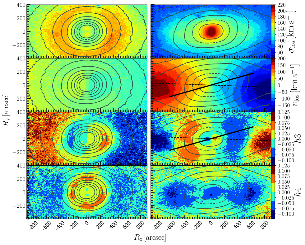
Figure 24: Kinematic maps and isophotes of model JR804 for the $\rm CB$ particles (left column) and the $\rm BPB$ and disc particles (right column). The isophotes are spaced every $\Delta\mu_{3.6}\,{\!=\!}\,0.5\,[{\rm mag}\,{\rm\,{\rm arcsec}^{-2}}]$ and the value $\mu_{3.6}\,{\!=\!}\,16\,[{\rm mag}\,{\rm\,{\rm arcsec}^{-2}}]$ is shown with a dashed isophote. In the $\rm BPB$ maps of $\upsilon_{\rm los}$ and $h3$ we show the projected bar major axis (solid line) and the projected disc major axis (dashed line). We exclude the isophotes in the centre to better reveal the central kinematic structures of each bulge component.

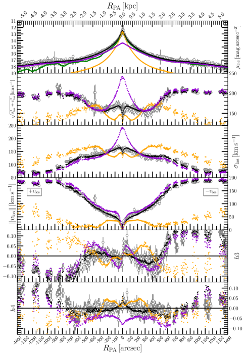
Figure 25: Surface-brightness and kinematic cuts near the disc major axis (${\rm PA}\,{\!=\!}\,33\degree$) of model JR804 (black dots) with its components, the $\rm CB$ (orange) and the $\rm BPB$ (purple), and of M31 (open circles). We also plot the extincted surface-brightness of the model observable $L^{A{\rm V}}$ ($\mu_{A{\rm V}}$, green line). Positive $R_{{\rm PA}}$ extends into the far side of the disc.

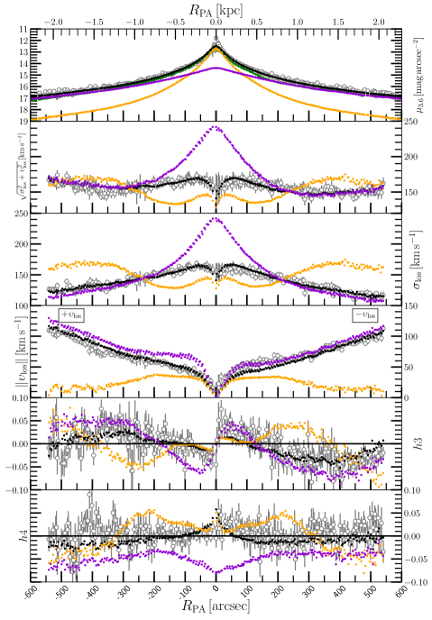
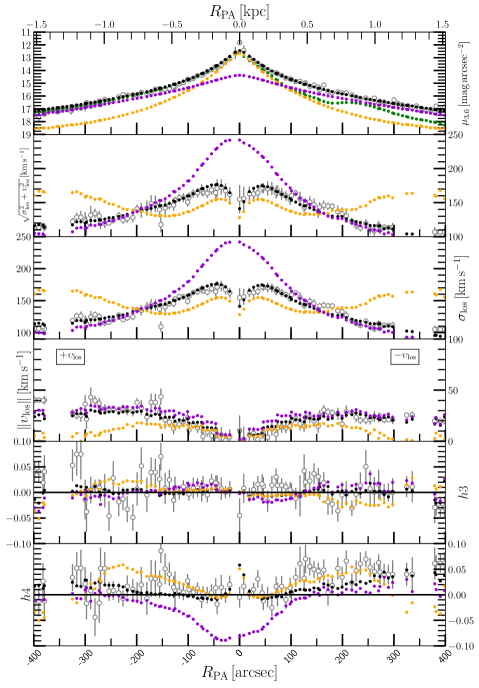
Figure 26: Surface-brightness and kinematic cuts along the projected bar major axis (${\rm PA}\,{\!=\!}\,55.7\degree$) in the left column and the bar minor axis (${\rm PA}\,{\!=\!}\,145.7\degree$) in the right column of model JR804 (black dots) with its components, the $\rm CB$ (orange) and the $\rm BPB$ (purple), and of M31 (open circles). We also plot the extincted surface-brightness of the model observable $L^{A{\rm V}}$ ($\mu_{A{\rm V}}$. green line). Positive $R_{{\rm PA}}$ extends into the near side of the disc.

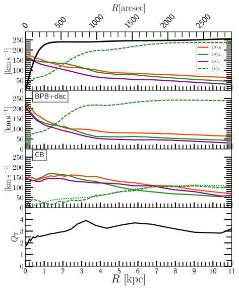
Figure 27: Intrinsic azimuthally averaged kinematic radial profiles in the disc plane for the best Einasto model for the total stellar components (top panel), $\rm BPB$ and disc (second panel), CB component (third panel), and the Toomre parameter $Q_{\rm T}$ (bottom panel). The dispersion profiles are shown in the first three panels in solid line for the coordinates $\langle\sigma\rangle_{R}$ (red), $\langle\sigma\rangle_{\phi}$ (green) and $\langle\sigma\rangle_{\rm z}$ (magenta), and the streaming velocity $\langle\upsilon\rangle_{\phi}$ is shown with a dashed green line. We also show $\langle\upsilon\rangle_{\phi}$ of the $\rm CB$ of Model 1 (green dotted line). The total circular velocity is shown in the first panel (black line).

In this section we present the bulge kinematics of the best model and compare them with the IFU kinematic measurements of O17.

For a better qualitative comparison we show kinematic maps in Figure 23, presenting the velocity, the dispersion, $h3$ and $h4$ of M31, the best model JR804 and the residuals. In Figure 24 we show separately the $\rm CB$ component and the $\rm BPB$ component of the best model. For an easier quantitative comparison we also show kinematic profiles along the disc major axis in Figure 25, and along the bar projected major and minor axis in Figure 26.

1. The line-of-sight dispersion ($\sigma_{\rm los}$): it has three important features that are reproduced by the model:

   1. Within $R<100\,{\rm arcsec}$ the velocity dispersion of M31 shows two peaks of $\sigma_{\rm los}^{\rm M31,max}\,{\!\sim\!}\,170\,{\rm km}\,{\rm s}^{\rm-1}$ along the bulge minor axis (O17), with a drop of $\sigma_{\rm los}$ in the centre. We find that this is produced by the concentrated $\rm CB$ that dominates in the centre (also shown in B17) which is revealed with the dispersion maps of each component in Fig 24, and in the $\sigma_{\rm los}$ profiles of Figure 25 and 26. The $\rm CB$ mass profile is similar to a Hernquist model, where the material in the centre requires lower kinetic energy to remain confined in gravitational equilibrium, leading to a dispersion drop. The two dispersion peaks, and partially the dispersion drop, can also be attributed to CB particles in circular orbits near the centre, as Hernquist (1990) shows for the Hernquist model. When plotted separately, the maximum central velocity dispersion of the $\rm CB$ alone is $\sigma_{\rm los}^{\rm CB,max}\,{\!\sim\!}\,150\,{\rm km}\,{\rm s}^{\rm-1}$, which combined with the high maximum central dispersion of the $\rm BPB$ with a peak of $\sigma_{\rm los}^{\rm BPB,max}\,{\!\sim\!}\,240\,{\rm km}\,{\rm s}^{\rm-1}$, reproduce the central dispersion in M31. A very important characteristic of the $\rm BPB$ is that its high central velocity dispersion is caused by the deep gravitational potential of the $\rm CB$ component, which due to its high mass concentration increases the central circular velocity. This results in particles orbiting the $\rm BPB$ and the thin bar that have high velocities when passing the centre.

   2. Our model also reproduces the two elongated high $\sigma_{\rm los}$ plateaus in the bulge noted by O17 within $R_{\rm x}\,{\!=\!}\,\pm 600\,{\rm arcsec}$ shown in Figures 23 and 26. This features are reproduced in the model by the $\rm BPB$ that dominates here over the classical bulge. At the end of the $\rm BPB$ along the projected bar major axis, or at the projected disc major axis at $R_{\rm x}\,{\!\sim\!}\,-600\,{\rm arcsec}$, the $\rm BPB$ surface-brightness is $\mu_{3.6}\,{\!\sim\!}\,17\,{\rm mag\,{\rm arcsec^{-2}}}$, while the $\rm CB$ is much fainter, with $\mu_{3.6}\,{\!\sim\!}\,18.5\,{\rm mag\,{\rm arcsec^{-2}}}$. The dispersion of the $\rm CB$ component in the outer part rises again. Further out the two $\sigma_{\rm los}$ plateaus end at $R_{\rm x}\,{\!\sim\!}\,\pm 600\,{\rm arcsec}$, decreasing along the major axis (Figure 23) to $\sigma_{\rm los}\,{\!\sim\!}\,70\,{\rm km}\,{\rm s}^{\rm-1}$ in the disc.

   3. Along the disc minor axis and at the near side of the disc (positive $R_{\rm y}$) the dispersion is systematically lower than the far side of the disc (negative $R_{\rm y}$) as shown by the maps (Figure 23) and the profiles (Figure 26). This feature is also reproduced in the model, and is caused by the dust absorption. This can be understood from Figure 21, and the dust extinction map in Figure 22: the light of the near side of the bulge that is behind the dust plane is strongly extinguished by the dust, leaving mostly the light of the foreground disc that has a dispersion lower than the bulge. In contrast, at negative $R_{\rm y}$, most of the light of the bulge is transmitted, while part of the light of the kinematically cooler disc material, which is now behind the bulge is absorbed, resulting in dispersions slightly higher than if the disc would be fully included. The dust also causes the observed asymmetry between the two $\sigma_{\rm los}$ plateaus, where for the side of $R_{\rm x}<0\,{\rm arcsec}$ the dispersion is higher than at the side of $R_{\rm x}>0\,{\rm arcsec}$.

2. The line-of-sight velocity ($\upsilon_{\rm los}$): We also find that the combination of both bulge components reproduces different characteristics of the M31 bulge velocity field, listing three of them below:

   1. In the very centre ($R<50\,{\rm arcsec}$) and near the disc major axis (${\rm PA}\,{\!=\!}\,33\degree$) (Figure 25) both bulge components show similar rotation ($\upsilon_{\rm los}\,{\!\sim\!}\,30\,{\rm km}\,{\rm s}^{\rm-1}$). However, at $R\,{\!\sim\!}\,100\,{\rm arcsec}$ the $\rm BPB$ rotates much faster, reaching already $\,{\!\sim\!}\,70\,{\rm km}\,{\rm s}^{\rm-1}$, while the $\rm CB$ component has $\,{\!\sim\!}\,35\,{\rm km}\,{\rm s}^{\rm-1}$, which then combined reproduce the total velocity of M31 with $\,{\!\sim\!}\,50\,{\rm km}\,{\rm s}^{\rm-1}$. Between 100$\,{\rm arcsec}$ and 600$\,{\rm arcsec}$ along the disc major axis, the $\rm BPB$ dominates the light and the rotation increases with a constant slope, reaching a roughly constant value of $\upsilon_{\rm los}\,{\!\sim\!}\,\pm 200\,{\rm km}\,{\rm s}^{\rm-1}$ in the disc region.

   2. Analysing the difference in velocity between the model and the observations in the panel $b$ of Figure 23, we find a region in the observations at $(R_{\rm x},R_{\rm y})\,{\!=\!}\,(200\,{\rm arcsec},100\,{\rm arcsec})$ that has a velocity $\,{\!\sim\!}\,10\,{\rm km}\,{\rm s}^{\rm-1}$ higher than the model. This is an asymmetry in the M31 observations that is not reproduced by our dust modelling. CO observations in this region (Melchior & Combes, 2011) indicate that the molecular gas kinematics is complex and maybe tilted in this region, and so it may be that our dust modelling is too simple here. As the bar major axis $\upsilon_{\rm los}$ profile shows (Figure 26), the $\rm BPB$ velocities match the observations well, suggesting that $\rm CB$ light contribution could be much weaker in this particular region.

   3. The velocity map (Figure 23) shows in the centre a twist in the zero velocity values that reproduces the velocity twist observed in M31. The twist is weaker in the very centre (within 100$\,{\rm arcsec}$) due to the $\rm CB$ component, which has a more oblate structure (Figure 24).

   4. The velocity of the CB component within 50$\,{\rm arcsec}$ is higher than the initial model before being fitted. As we show later in Figure 27, the CB component of the initial model gain rotation from the bar, but mostly in the outer parts. This could mean that the observed high central rotation could be a legacy from the early formation of the CB.

3. The Gauss-Hermite coefficients $h3$ and $h4$:

   1. The $h3$ maps (Figure 23) and profiles (Figure 26) show that the $h3$ values in the disc region beyond $R_{\rm x}\!>\!700\,{\rm arcsec}$ and $R_{\rm x}\!<\!-700\,{\rm arcsec}$ are anti-correlated with the velocity $\upsilon_{\rm los}$, changing when we enter the region of the bar, with $h3$ then correlated with the velocity. This behaviour is expected in barred galaxies (Bureau & Athanassoula, 2005; Iannuzzi & Athanassoula, 2015). However, the central region of M31’s bulge has a second change of sign in $h3$, which is also reproduced by the model (i.e. $h3$ and $\upsilon_{\rm los}$ are again anti-correlated for isophotes with $\mu_{3.6}\!\leq\!16.5\,{\rm mag\,{\rm arcsec^{-2}}}$). This central $h3-\upsilon_{\rm los}$ anti-correlation feature is produced by both bulge components, and it is due to the near axisymmetric central density distribution, similar to the way that the asymmetric drift causes the $h3-\upsilon_{\rm los}$ anti-correlation in the axisymmetric disc. The dust extinction also generates an asymmetry between the $h3$ at the left and the right side of the bar that is reproduced by the model (Figure 23). In particular, the $h3-\upsilon_{\rm los}$ correlation in the bar region is more extended along the $R_{\rm x}$ axis in the positive side of $R_{\rm x}$. This is because a large fraction of light from the bar at negative $R_{\rm x}$ is behind the dust and it is more strongly absorbed, leaving the foreground part of the disc component more visible.

   2. The M31 $h4$ map in Figure 23 reveals in the centre a positive region, while at the end of the $\rm BPB$ ($R_{\rm x}\,{\!\sim\!}\,\pm 600\,{\rm arcsec}$) the $h4$ map shows negative values. In the model the $\rm BPB$ $h4$ map in Figure 24 shows mostly negative values, and the central positive $h4$ region is reproduced by the $\rm CB$ that shows strong positive $h4$ (except where the two $\sigma_{\rm los}$ peaks are detected, where the classical bulge $h4$ is negative). Along the disc minor axis $h4$ has positive values at $R_{\rm y}\,{\!=\!}\,\pm 400\,{\rm arcsec}$, with larger positive values in the near side of the disc, which is where the dust extinction effects are stronger. Our $h4$ maps also agree with the results for other box/peanut bulge models (Iannuzzi & Athanassoula, 2015), where $h4$ depends on the bar angle for bars with strong box/peanut bulges, while bars with weak or without a box/peanut bulges show a weaker dependence.

4. Stellar kinematics in the outer disc and the inner spheroid:
   In Figure 27 we show the de-projected kinematic profiles of the best Einasto model. We also show the Toomre parameter $Q_{\rm T}\,{\!=\!}\,\kappa\,\langle\sigma\rangle_{r}\left(3.36\,G\,\Sigma\left(R\right)\right)^{-1}$ (Toomre, 1964) calculated with the azimuthally averaged surface mass density profile $\Sigma\left(R\right)$ and the radial velocity dispersion $\langle\sigma\rangle_{r}$ from the disc particles and the epicycle frequency $\kappa$ from the total circular velocity. The stellar disc is stable and dynamically hot with a radially averaged value and standard deviation of $\langle Q_{\rm T}\rangle\,{\!=\!}\,2.6\!\pm\!0.6$. This is consistent with Dorman et al. (2015, see their Figure 16) who also find that M31 has a dynamically hot stellar disc.
   

   The intrinsic kinematic profiles in Figure 27 also shows that in the outer parts the $\rm CB$ increases its rotation to $\,{\!\sim\!}\,70\,{\rm km}\,{\rm s}^{\rm-1}$ at 5$\,{\rm kpc}$, similar to the values estimated for the inner spheroidal component at that radius (Dorman et al., 2012), reaching $\,{\!\sim\!}\,100\,{\rm km}\,{\rm s}^{\rm-1}$ at 10$\,{\rm kpc}$. The outer rotation of the $\rm CB$ is similar to the Model 1 of B17, which obtained all its rotation from the angular momentum transfer from the bar (Saha et al., 2016). The increase of the rotation of the inner spheroid at this radius is not unexpected, as for example it is also observed in the Milky Way’s inner stellar halo (Ness et al., 2013; Perez-Villegas et al., 2017).
   

5. Stellar and globular cluster kinematics:
   Given that the kinematic properties of each bulge component are different, is there a signature or tracer which could identify each stellar component observationally? Morrison et al. (2011) analyse velocities and metallicities of a sample of old star clusters near the M31 centre, concluding that these clusters could be associated with the bar or the inner spheroid depending on their metallicities: the more metal-rich clusters $(\,{\rm Z/H}\!\geq\!-0.6\,{\rm dex})$ near the disc major axis beyond $R\,{\!\sim\!}\,4\,{\rm kpc}$ have velocities similar to the M31 surrounding field stars ($\,{\!\sim\!}\,200\,{\rm km}\,{\rm s}^{\rm-1}$), but within the $\rm BPB$ region ($R<2\,{\rm kpc}$), the clusters reach higher velocities ($\,{\!\sim\!}\,300\,{\rm km}\,{\rm s}^{\rm-1}$) similar to the $\rm BPB$ velocity dispersion presented here. Given that they assumed that the bar is roughly edge on ($\theta_{\rm bar}\,{\!\sim\!}\,20\degree$) they associate the metal-rich component with the $x_{2}$ orbits that are perpendicular to the bar. However, in B17 and here we find $\theta_{\rm bar}\,{\!\sim\!}\,55\degree$ with the end of the thin bar in projection at $R\,{\!=\!}\,2.3\,{\rm kpc}\,(600\,{\rm arcsec})$, approximately the location where the metal-rich star clusters velocity changes. The more metal-poor clusters $(\,{\rm Z/H}\!\leq\!-0.8\,{\rm dex})$ show less co-rotation with the field stars with a broader velocity distribution, similar to the outer classical bulge kinematic properties, or to a spheroid component like the inner stellar halo. Therefore, the bulge models presented here support the scenario where the star clusters in the centre could be associated with different stellar components.

3.2.5 Kinematics: circular velocity & the Lindblad resonances.

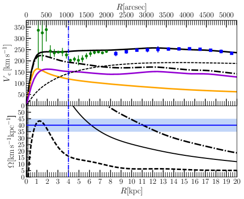
Figure 28: Top panel: azimuthally averaged circular velocity in the plane of the disc of the model JR804 with the different components: the $\rm CB$ (orange), the $\rm BPB$ and the stellar disc (purple), the total stellar component (dot dashed line), the dark matter (dash) and the total circular velocity (solid black). The H I data of Corbelli et al. (2010) is shown out to 20$\,{\rm kpc}$ (blue squares). We also show the H I data of Chemin et al. (2009) within 8$\,{\rm kpc}$ (green circles). Bottom panel: the angular frequency profile $\Omega$ (solid curve), $\Omega_{\rm ILR}\,{\!=\!}\,\Omega-\kappa/2$ (dash curve), and $\Omega_{\rm OLR}\,{\!=\!}\,\Omega+\kappa/2$ of the model JR804 with a bar pattern speed ${\Omega_{\rm p}\!=\!40\pm 5\,{\rm km}\,{\rm s}^{\rm-1}\,{\rm kpc}^{-1}}$(blue horizontal line and shaded region). The corotation radius, the Lindblad resonances inner inner, outer inner, and outer are located at $r_{\rm cor}\,{\!=\!}\,6.5\pm 1.0\,{\rm kpc}$, $r_{\rm IILR}\,{\!=\!}\,1.0\,{\rm kpc}$, $r_{\rm OILR}\,{\!=\!}\,1.8\,{\rm kpc}$ and $r_{\rm OLR}\,{\!=\!}\,11.2\pm 1.0\,{\rm kpc}$. The end of the thin bar (B17) is shown in both panels (blue vertical dotted dashed line).

In Figure 28 we show the total circular velocity $V_{\rm c}$ profile of the best model JR804 with its different components. The $\rm CB$ component reaches a maximum circular velocity of $V_{\rm c}^{\rm CB,max}\,{\!=\!}\,165\,{\rm km}\,{\rm s}^{\rm-1}$ at 1.0$\,{\rm kpc}$, dominating over the $\rm BPB$ component within $R\!\leq\!0.5\,{\rm kpc}$, and then drops nearly Keplerianly. The $\rm BPB$ component reaches a maximum of $V_{\rm c}^{\rm BPB,max}\,{\!=\!}\,160\,{\rm km}\,{\rm s}^{\rm-1}$ at 2.0$\,{\rm kpc}$, where it dominates over the classical bulge, which has 140$\,{\rm km}\,{\rm s}^{\rm-1}$ at that radius. The total circular velocity increases fast due to the $\rm CB$ contribution, reaching $V_{\rm c,o}\,{\!=\!}\,235\,{\rm km}\,{\rm s}^{\rm-1}$ at 1.6$\,{\rm kpc}$ where it stays roughly flat reaching a maximum of $V_{\rm c,max}\,{\!=\!}\,255\,{\rm km}\,{\rm s}^{\rm-1}$ at $\,{\!\sim\!}\,$ 12.5$\,{\rm kpc}$. We also show the H I rotation curve of Corbelli et al. (2010) that is used to fit the dark matter density profile, which is in general well fitted. The authors neglect the inner $R<8.5\,{\rm kpc}$, arguing the presence of an inner warp and the non-circular motion of the gas. For comparison we also show the inner $R<8\,{\rm kpc}$ of the H I rotation curve from Chemin et al. (2009) although we similarly caution about the non-axisymetric motion of the gas here.

In the bottom panel of Figure 28 we show the angular frequency profile ($\Omega$) of the best model, with the range of best bar pattern speed ${\Omega_{\rm p}\!=\!40\pm 5\,{\rm km}\,{\rm s}^{\rm-1}\,{\rm kpc}^{-1}}$. The corotation radius, where ${\Omega_{\rm p}\,\,}\,{\!=\!}\,\Omega$, is located at $r_{\rm cor}\,{\!=\!}\,6.5\pm 1.0\,{\rm kpc}$. The isophotal comparison of the M31 bulge with N-body models in B17 suggests that the thin bar length of M31 is $r_{\rm bar}^{\rm thin}\,{\!\sim\!}\,4.0\,{\rm kpc}$, which would classify M31’s bar as a slow bar with $\mathcal{R}\,{\!=\!}\,1.6\pm 0.2$, where Debattista & Sellwood (2000) define slow bars to be when $\mathcal{R}\,{\!=\!}\,r_{\rm cor}/r_{\rm bar}^{\rm thin}\!\leq\!1.4$ . The inner inner and the outer inner Lindblad resonances ($\Omega_{\rm ILR}\,{\!=\!}\,\Omega-\kappa/2$ Lindblad, 1956), in this model are located at $r_{\rm IILR}\,{\!=\!}\,1.0\,{\rm kpc}$ and $r_{\rm OILR}\,{\!=\!}\,1.8\,{\rm kpc}$. The outer Lindblad resonance $\Omega_{\rm OLR}\,{\!=\!}\,\Omega+\kappa/2$ is then at $r_{\rm OLR}\,{\!=\!}\,11\pm 1\,{\rm kpc}$.

The gas kinematics and its distribution in M31 shows many substructures that are consistent with the typical properties observed in other barred galaxies. In the centre of the bulge between $\,{\!\sim\!}\,$ 1$\,{\rm kpc}$ (260$\,{\rm arcsec}$) and $\,{\!\sim\!}\,$ 2$\,{\rm kpc}$ (500$\,{\rm arcsec}$) the gas velocity measured by Chemin et al. (2009) reaches $\,{\!\sim\!}\,340\,{\rm km}\,{\rm s}^{\rm-1}$, higher than the circular velocity $V_{\rm c}\,{\!\sim\!}\,230\,{\rm km}\,{\rm s}^{\rm-1}$. However, this difference is expected in barred galaxies where the gas has a non-circular motion with in-falling streams of gas, as shown by Kim et al. (2012, see their Figure 5, see also ). Such streams are typically located near the inner Lindblad resonances, which in this model are at $r_{\rm IILR}\,{\!=\!}\,1.0\,{\rm kpc}\,(260\,{\rm arcsec})$ and $r_{\rm OILR}\,{\!=\!}\,1.8\,{\rm kpc}\,(470\,{\rm arcsec})$, almost exactly where O17 also detects the presence of high velocity streams of gas with $\,{\!\sim\!}\,\pm 300\,{\rm km}\,{\rm s}^{\rm-1}$.

A second signature is that the H I gas velocity drops in the transition between the bar and the disc, as observed between 4$\,{\rm kpc}$ and 6$\,{\rm kpc}$. This again is typically produced in barred galaxy simulations due to the non circular motion of the gas in the non axisymmetric potential produced by the bar.

Finally, there is the 10$\,{\rm kpc}$ ring-like substructure (Habing et al., 1984; Gordon et al., 2006; Barmby et al., 2006). This is made of stars, gas and dust and it is where most of the current star formation occurs (Ford et al., 2013; Rahmani et al., 2016), with a star formation timescale longer than 500$\,{\rm Myr}$ (Lewis et al., 2015). This is longer than the dynamical time scale at this radius, making an ephemeral collision origin unlikely, as proposed by Block et al. (2006); Dierickx et al. (2014) (see however Hammer et al., 2018). Assuming that this structure is located at 10$\,{\rm kpc}$ and that it is related to a resonance with the bar, B17 predict a bar pattern speed of ${\Omega_{\rm p}\,\,}\,{\!=\!}\,41\,{\rm km}\,{\rm s}^{\rm-1}\,{\rm kpc}^{-1}$. Here we use the bulge stellar kinematics as fitting constraints, finding ${\Omega_{\rm p}\!=\!40\pm 5\,{\rm km}\,{\rm s}^{\rm-1}\,{\rm kpc}^{-1}}$, placing the outer Lindblad resonance at $r_{\rm OLR}\,{\!=\!}\,11\pm 1\,{\rm kpc}$ near the ring structure. This suggests that the OLR could be related to the formation of the ring, as also observed in other galaxies (Buta & Crocker, 1991; Buta, 2017).

4 Summary and discussion

We have presented here dynamical models for M31 built with a classical bulge component ($\rm CB$) and a box/peanut bulge component ($\rm BPB$). We use the M2M method to measure the main properties of M31’s bulge: the IRAC 3.6${\rm\mu m}$ mass-to-light ratio ${\Upsilon_{3.6}\,\,}$, the dark matter mass within 3.2$\,{\rm kpc}$ of the bulge ${M^{\rm B}_{\rm DM}\,\,}$, and the pattern speed of the $\rm BPB$ and the thin bar ${\Omega_{\rm p}\,\,}$. For this we directly fit simultaneously new IFU VIRUS-W bulge stellar kinematic observations (Opitsch et al., 2017), and the 3.6${\rm\mu m}$ IRAC photometric data (Barmby et al., 2006), with the following main results:

1. The range of parameters that best reproduce all the observations simultaneously are ${\Upsilon_{3.6}\!=\!0.72\!\pm\!0.02\,{\rm M_{\odot}\,L_{\odot}^{-1}}\,}$, ${\Omega_{\rm p}\!=\!40\pm 5\,{\rm km}\,{\rm s}^{\rm-1}\,{\rm kpc}^{-1}}$and ${M^{\rm B}_{\rm DM}\!=\!1.2^{+0.2}_{-0.4}\times 10^{10}\,{\rm M_{\odot}}\,}$, using an Einasto dark matter profile. These models have a total dynamical mass within the composite bulge of $M_{\rm dyn}^{\rm B}\,{\!=\!}\,4.25^{+0.10}_{-0.29}\times 10^{10}\,{\rm M_{\odot}}$ with a stellar mass and percentage of $M_{\star}^{\rm B}\,{\!=\!}\,3.09^{+0.10}_{-0.12}\times 10^{10}\,{\rm M_{\odot}}$(73%). The CB has $M_{\star}^{\rm CB}\,{\!=\!}\,1.18^{+0.06}_{-0.07}\times 10^{10}\,{\rm M_{\odot}}$(28%) and the $\rm BPB$ has $M_{\star}^{\rm BPB}\,{\!=\!}\,1.91\pm 0.06\times 10^{10}\,{\rm M_{\odot}}$(45%). We also obtain similar values within the errors for our grid of models with NFW dark matter haloes. The bulge dark matter mass agrees with the expected values for an adiabatically contracted NFW halo with M31’s virial mass. However, the best Einasto models fit the bulge stellar kinematics generally better than the models with NFW haloes, favouring a shallow central dark matter halo distribution, similar to that found in the Milky Way (Portail et al., 2017a). This also reveals the importance of kinematic data with high spectral and spatial resolution, and the appropriate modelling to accurately determine the central dark matter mass distribution in galaxies.

2. How does the model of B17 compare with the best M2M models? They explored N-body simulations build with $\rm CB$ components of different masses and sizes, where the $\rm BPB$ formed from the bar instabilities of the initial disc during the simulations. They find a best model selected from photometric comparisons with M31’s bulge. Here we improve the models of B17 by fitting directly the data using the M2M method. The main properties of their $\rm CB$ are similar to the ones found here. The B17 $\rm BPB$ luminosity is also similar to the value presented here, however, given their slightly larger mass-to-light ratio their $\rm BPB$ mass is 15 per cent higher. Their kinematic maps qualitatively match several features observed in M31, however the M2M model highly improves the match quantitatively. For example, the M2M model presented here reproduces now the velocity dispersion in the outer parts of the $\rm BPB$ due to a more massive dark matter halo.

3. Our best model has two bulge components with completely different kinematics that only together successfully reproduce the detailed properties of the kinematic and the photometric maps. Furthermore, our modelling includes dust absorption effects that can approximately reproduce the kinematic asymmetries in the observations. The model, for example, reproduces the higher dispersion of the far side of the galaxy compared to the near side.

4. Our results present new constraints on the early formation of M31 given the lower mass found for the $\rm CB$ component compared to previous estimations in the literature. An implication is on the relation between bulges and central super massive black holes (SMBH). SMBH masses show correlations with classical bulges and not pseudobulges (Hu, 2008; Kormendy & Ho, 2013; Saglia et al., 2016).

   Using the $M_{\bullet}\!-\!M_{\rm bulge}\!-\!\sigma$ relation from Saglia et al. (2016) for the $\rm CB$ component alone with a mass of $M_{\star}^{\rm CB,10\,{\rm kpc}}\,{\!=\!}\,1.71\times 10^{10}\,{\rm M_{\odot}}$ with $\sigma^{\rm CB,max}\,{\!\sim\!}\,130$ - $150\,{\rm km}\,{\rm s}^{\rm-1}$ predicts a SMBH mass of $M_{\bullet}\,{\!=\!}\,0.4^{+0.4}_{-0.2}\,-\,0.6^{+0.7}_{-0.3}\times 10^{8}\,{\rm M_{\odot}}$, where the errors are the instrinsic scatter in the relation. This is somewhat lower than the measured $M_{\bullet}\,{\!=\!}\,1.4^{+0.9}_{-0.3}\times 10^{8}\,{\rm M_{\odot}}$ (Bender et al., 2005), but lies within the scatter. Using the $M_{\bullet}\!-\!M_{\rm bulge}\,{}^{3}$ relation predicts a mass of $M_{\bullet}\,{\!=\!}\,0.9^{+1.5}_{-0.5}\times 10^{8}\,{\rm M_{\odot}}$, that is closer to the measured value in M31.

5. The tightly constrained stellar mass-to-light ratio value of ${\Upsilon_{3.6}\!=\!0.72\!\pm\!0.02\,{\rm M_{\odot}\,L_{\odot}^{-1}}\,}$is in agreement with the expected values from stellar populations with a Chabrier IMF (Meidt et al., 2014), with the metallicities and ages measured in M31’s bulge and bar (Opitsch, 2016; Saglia et al., 2018). Considering the $\rm CB$ alone a Chabrier IMF would be consistent with Cappellari et al. (2012) (using $\Upsilon_{\rm r}\,{\!\sim\!}\,4\,{\rm M_{\odot}\,L_{\odot}^{-1}}$ and $\sigma_{\rm CB}\,{\!\sim\!}\,150\,{\rm km}\,{\rm s}^{\rm-1}$). It is however inconsistent with the Salpeter IMF found for more massive classical bulges measured by Dutton et al. (2013, SWELLS survey).

6. Our findings agree with the photometric (Fisher & Drory, 2008) and kinematic (Fabricius et al., 2012) bulge classification criteria using the Sérsic index ($n$) and the central kinematics to distinguish classical bulges ($n>2$) from pseudobulges ($n<2$). As Fisher & Drory (2008) mention, and Erwin et al. (2015) investigate further, composite bulges can have an effect on the bulge selection criteria, and they can manifest both bulge type properties. Here we find that M31’s composite bulge Sérsic index is at the boundary with $n_{\rm M31}\,{\!\sim\!}\,2$ and it shows kinematic properties of both bulge types. Moreover, considering the $\rm CB$ alone we find $n_{\rm CB}\,{\!\sim\!}\,4$, a $\rm CB$ to total mass ratio ${\rm B}/{\rm T}\,{\!=\!}\,0.21$, effective radius $R_{\rm e}^{\rm CB}\,{\!\sim\!}\,1\,{\rm kpc}$, and central dispersion $\sigma_{\rm CB}\,{\!\sim\!}\,150\,{\rm km}\,{\rm s}^{\rm-1}$, which also agree with the criteria for classical bulge types.

   Here we present two properties of a composite bulge that could improve the selection criteria: i) a composite bulge with $n\!\approx\!2$ can host a classical bulge with a high Sérsic index, where the composite bulge has a value lowered by the presence of a box/peanut bulge, and ii) the presence of a classical bulge component can increase the total central dispersion by increasing the dispersion of the box/peanut bulge that lives within the classical bulge potential. This suggests that other observed bulges that show low Sérsic values ($n\lesssim 2$), but with high central dispersion and a large dispersion gradient ($\nabla\sigma$) (Neumann et al., 2017), could be hosting a compact classical bulge.

7. Our best M31 bar pattern speed value is ${\Omega_{\rm p}\!=\!40\pm 5\,{\rm km}\,{\rm s}^{\rm-1}\,{\rm kpc}^{-1}}$ which results in $\mathcal{R}\,{\!=\!}\,1.6\pm 0.2$, placing this bar among the slow bars. This is within the range of recent measurements of $\mathcal{R}$ of barred galaxies, finding $\mathcal{R}\,{\!=\!}\,1.41\pm 0.26$ (Spitzer with gas kinematics Font et al., 2017) and $\mathcal{R}\,{\!=\!}\,1.0^{+0.7}_{-0.4}$ (CALIFA survey Aguerri et al., 2015). Furthermore, our pattern speed measurement places the inner Lindblad resonances near the inner gas rings and streams observed within the bulge (Opitsch et al., 2017), and the outer Lindblad resonance near the 10$\,{\rm kpc}$ ring, which could explain its origin and persisting star forming activity (Lewis et al., 2015).

Finally, the M2M models presented here have many possible uses. They can be applied to investigate further the early formation and the secular evolution of M31. For example, including gas to reproduce the outer 10$\,{\rm kpc}$ ring-like substructure, or the bulge gas distribution. Also, from stellar population and chemodynamical galaxy formation simulations (Kobayashi & Nakasato, 2011) it is expected that the stars with different chemical elements have different spatial distributions. The M31 bulge metallicity maps (Saglia et al., 2018) could be used to dissect the galaxy’s orbital structure using a chemodynamical modelling, as similarly done for the MW (Portail et al., 2017b). Other applications of our model involve the interpretation of pixel micro-lensing events in M31’s halo for the observational campaigns PAndromeda (Lee et al., 2012) and WeCAPP (Lee et al., 2015). For the pixel lensing modelling an important ingredient are accurate dynamical models of the stellar mass distribution to take into account the self-lensing events, and thereby better constrain the lensing events in the halo (Riffeser et al., 2006). The models presented here are the most appropriate as these include the barred nature of the Andromeda galaxy.
These models may be available upon request to the authors.

Appendix A NFW grid of parameters and Einasto cube of parameters

References

- Abadi et al. (2010) Abadi M. G., Navarro J. F., Fardal M., Babul A., Steinmetz M., 2010, MNRAS, 407, 435
- Aguerri et al. (2015) Aguerri J. A. L., Sánchez S. F., Husemann B., Mast D., 2015, A&A, 576, 102
- Athanassoula & Beaton (2006) Athanassoula E., Beaton R. L., 2006, MNRAS, 370, 1499
- Athanassoula & Misiriotis (2002) Athanassoula E., Misiriotis A., 2002, MNRAS, 330, 35
- Athanassoula et al. (2016) Athanassoula E., Rodionov S. A., Peschken N., Lambert J. C., 2016, ApJ, 821
- Baes & Dejonghe (1999) Baes M., Dejonghe H., 1999, MNRAS, 313, 153
- Barmby et al. (2006) Barmby P., et al., 2006, ApJ, 650, L45
- Beaton et al. (2007) Beaton R. L., et al., 2007, ApJ, 658, L91
- Bender et al. (1994) Bender R., Saglia R. P., Gerhard O. E., 1994, MNRAS, 269
- Bender et al. (2005) Bender R., et al., 2005, ApJ, 631, 280
- Berman (2001) Berman S., 2001, A&A, 371, 476
- Berman & Loinard (2002) Berman S., Loinard L., 2002, MNRAS, 336, 477
- Binney et al. (1991) Binney, J., Gerhard, O. E., Stark, A. A., Bally, J., & Uchida, K. I. 1991, MNRAS, 252, 210
- Blaña et al. (2017) Blaña M., Wegg C., Gerhard O., Erwin P., Portail M., Opitsch M., Saglia R., Bender R., 2017, MNRAS, 466, 4279
- Bland-Hawthorn & Gerhard (2016) Bland-Hawthorn J., Gerhard O., 2016, Annu. Rev. Astron. Astrophys., 54, 529
- Block et al. (2006) Block D. L., et al., 2006, Nature, 443, 832
- Blumenthal et al. (1986) Blumenthal G. R., Faber S. M., Flores R., Primack J. R., 1986, pp 27–34
- Bournaud et al. (2005) Bournaud F., Jog C. J., Combes F., 2005, A&A, 437, 69
- Brinks, E.; Burton (1984) Brinks, E.; Burton W. B., 1984, A&A, 141, 195
- Bureau & Athanassoula (2005) Bureau M., Athanassoula E., 2005, ApJ, 626, 159
- Buta (2017) Buta R. J., 2017, ] 10.1093/mnras/stx1392, 3849, 3819
- Buta & Crocker (1991) Buta R., Crocker D. A., 1991, Astron. J., 102, 1715
- Capaccioli (1989) Capaccioli M., 1989, 1989, world galaxies; Proc. Conf. New York Springer-Verlag, 208, eds Corwin Jr. H.G. Bottinelli L.
- Cappellari et al. (2012) Cappellari M., et al., 2012, Nature, 484, 485
- Chemin et al. (2009) Chemin L., Carignan C., Foster T., 2009, ApJ, 705, 1395
- Chemin et al. (2015) Chemin L., Renaud F., & Soubiran C., 2015, A&A, 578A, 14C
- Combes et al. (1990) Combes F., Debbasch F., Friedli D., Pfenniger D., 1990, Astron. Astrophys. (ISSN 0004-6361), 233, 82
- Corbelli et al. (2010) Corbelli E., Lorenzoni S., Walterbos R., Braun R., Thilker D., 2010, A&A, 511, A89
- Correa et al. (2015a) Correa C. A., Wyithe J. S. B., Schaye J., Duffy A. R., 2015a, MNRAS, 450, 1514
- Correa et al. (2015b) Correa C. A., Stuart J., Wyithe B., Schaye J., Duffy A. R., 2015b, MNRAS, 452, 1217
- Courteau et al. (2011) Courteau S., Widrow L. M., McDonald M., Guhathakurta P., Gilbert K. M., Zhu Y., Beaton R. L., Majewski S. R., 2011, ApJ, 739, 20
- Dalcanton et al. (2015) Dalcanton J. J., et al., 2015, ApJ, 814, 47
- De Lorenzi et al. (2007) De Lorenzi F., Debattista V. P., Gerhard O., Sambhus N., 2007, MNRAS, 376, 71
- De Lorenzi et al. (2008) De Lorenzi F., Gerhard O., Saglia R. P., Sambhus N., Debattista V. P., Pannella M., Méndez R. H., 2008, MNRAS, 385, 1729
- Debattista & Sellwood (2000) Debattista V. P., Sellwood J. A., 2000, ApJ, 543, 704
- Debattista et al. (2006) Debattista V. P., Mayer L., Carollo C. M., Moore B., Wadsley J., Quinn T., 2006, ApJ, 645, 209
- Dierickx et al. (2014) Dierickx M., Blecha L., Loeb A., 2014, ApJ, 788, L38
- Dorman et al. (2012) Dorman C. E., et al., 2012, ApJ, 752, 147
- Dorman et al. (2015) Dorman C. E., et al., 2015, ApJ, 803, 24
- Draine & Li (2007) Draine B. T., Li A., 2007, ApJ, 657, 810
- Draine et al. (2014) Draine B. T., et al., 2014, ApJ, 780, 172
- D’Souza & Bell (2018) D’Souza R., & Bell E.F., 2018, Nat.As, 102D
- Dutton et al. (2011) Dutton A. A., et al., 2011, MNRAS, 416, 322
- Dutton et al. (2013) Dutton A. A., et al., 2013, MNRAS, 428, 3183
- Einasto (1965) Einasto J., 1965, Tr. Astrofiz. Instituta Alma-Ata, Vol. 5, 87
- Erwin (2015) Erwin P. M. P. I. f. e. P., 2015, ApJ, 799, 26
- Erwin (2017) Erwin P., 2017, MNRAS, 474, 5372
- Erwin & Debattista (2016) Erwin P., Debattista V. P., 2016, Astrophys. J. Lett., 825, L30
- Erwin & Debattista (2017) Erwin P., Debattista V. P., 2017, MNRAS, 468, 2058
- Erwin et al. (2008) Erwin P., Pohlen M., Beckman J. E., 2008, Astron. J., 135, 20
- Erwin et al. (2015) Erwin P., et al., 2015, MNRAS, 446, 4039
- Fabricius et al. (2012) Fabricius M. H., Saglia R. P., Fisher D. B., Drory N., Bender R., Hopp U., 2012, ApJ, 754, 67
- Fisher & Drory (2008) Fisher D. B., Drory N., 2008, Astron. J., 136, 773
- Font et al. (2017) Font J., et al., 2017, ApJ, 835, 1
- Ford et al. (2013) Ford G. P., et al., 2013, ApJ, 769, 55
- Gebhardt et al. (2003) Gebhardt K., et al., 2003, ApJ, 583, 92
- Gerhard & Vietri (1986) Gerhard O.E., Vietri M., 1986, MNRAS, 223, 377
- Gerhard (1993) Gerhard O. E., 1993, MNRAS, 265
- Gordon et al. (2006) Gordon K. D., et al., 2006, ApJ, 638, L87
- Habing et al. (1984) Habing H. J., et al., 1984, ApJ, 278, L59
- Hammer et al. (2010) Hammer F., Yang Y. B., Wang J. L., Puech M., Flores H., Fouquet S., 2010, ApJ, 725, 542
- Hammer et al. (2018) Hammer F., Yang Y. B., Wang J. L., Ibata R., Flores H., Puech M., 2018, Mon. Not. R. Astron. Soc.
- Henderson (1979) Henderson A. P., 1979, A&A, 75, 311
- Hernquist (1990) Hernquist L., 1990, ApJ, 356, 359
- Hu (2008) Hu J., 2008, MNRAS, 386, 2242
- Iannuzzi & Athanassoula (2015) Iannuzzi F., Athanassoula E., 2015, MNRAS, 450, 2514
- Jedrzejewski (1987) Jedrzejewski R. I., 1987, MNRAS, 226, 747
- Kent (1989) Kent S. M., 1989, Astron. J., 97, 1614
- Kim et al. (2012) Kim W.-T., Seo W.-Y., Stone J. M., Yoon D., Teuben P. J., 2012, ApJ, 747, 60
- Kim et al. (2014) Kim T., et al., 2014, ApJ, 782, 64
- Kobayashi & Nakasato (2011) Kobayashi C., Nakasato N., 2011, ApJ, 729
- Koleva et al. (2011) Koleva M., Prugniel P., De Rijcke S., Zeilinger W. W., 2011, MNRAS, 417, 1643
- Kormendy (2013) Kormendy J., 2013, Cambridge Univ. Press. p.1, eds. J. Falcon-Barroso J. H. Knapen
- Kormendy & Ho (2013) Kormendy J., Ho L. C., 2013, , ARA&A, 51, 511
- Lee et al. (2012) Lee C. H., et al., 2012, Astron. J., 143
- Lee et al. (2015) Lee C.-H., Riffeser A., Seitz S., Bender R., Koppenhoefer J., 2015, ApJ, 806, 161
- Lewis et al. (2015) Lewis A. R., et al., 2015, ApJ, 805
- Li et al. (2015) Li Z., Shen J., Kim W.-T., 2015, ApJ, 806, 150
- Lindblad (1956) Lindblad B., 1956, Stock. Obs. Ann., 19, 2
- Long & Mao (2010) Long R. J., Mao S., 2010, MNRAS, 405, 301
- Martinez-Valpuesta (2012) Martinez-Valpuesta I., 2012, Dyn. Meets Kinematic Tracers, Online http//mpia.de/~dynamics/ringberg/?view=program, id.12
- McConnachie et al. (2005) McConnachie A. W., Irwin M. J., Ferguson A. M. N., Ibata R. A., Lewis G. F., Tanvir N., 2005, MNRAS, 356, 979
- Meidt et al. (2014) Meidt S. E., et al., 2014, ApJ, 788, 144
- Melchior & Combes (2011) Melchior A.-L., Combes F., 2011, A&A, 536, 19
- Menendez-Delmestre et al. (2007) Menendez-Delmestre K., Sheth K., Schinnerer E., Jarrett T. H., Scoville N. Z., 2007, ApJ, 657, 790
- Morganti & Gerhard (2012) Morganti L., Gerhard O., 2012, MNRAS, 422, 1571
- Morganti et al. (2013) Morganti L., Gerhard O., Coccato L., Martinez-Valpuesta I., Arnaboldi M., 2013, MNRAS, 431, 3570
- Morrison et al. (2011) Morrison H., Caldwell N., Schiavon R. P., Athanassoula E., Romanowsky A. J., Harding P., 2011, ApJ, 726, L9
- Naab & Burkert (2003) Naab T., Burkert A., 2003, ApJ, 597, 893
- Navarro et al. (1996) Navarro J. F., Frenk C. S., White S. D. M., 1996, ApJ, 462, 563
- Ness et al. (2013) Ness M., et al., 2013, MNRAS, 432, 2092
- Neumann et al. (2017) Neumann J., et al., 2017, A&A, 604, 1
- Newton & Emerson (1977) Newton K., Emerson D. T., 1977, MNRAS, 181, 573
- Oh et al. (2008) Oh S.-H., de Blok W. J. G., Walter F., Brinks E., Kennicutt R. C., 2008, Astron. J., 136, 2761
- Opitsch (2016) Opitsch M., 2016, PhD thesis, LMU München, https://edoc.ub.uni-muenchen.de/20107/
- Opitsch et al. (2017) Opitsch M., Fabricius M. H., Saglia R. P., Bender R., Blaña M., Gerhard O., 2017, eprint arXiv:1707.06652
- Perez-Villegas et al. (2017) Perez-Villegas A., Portail M., Gerhard O., 2017, MNRAS, 464, L80
- Planck Collaboration et al. (2013) Planck Collaboration et al., 2013, Astron. Astrophys. Vol. 571, id.A16, 66 pp., 571
- Portail et al. (2015) Portail M., Wegg C., Gerhard O., Martinez-Valpuesta I., 2015, MNRAS, 448, 713
- Portail et al. (2017a) Portail M., Gerhard O., Wegg C., Ness M., 2017a, MNRAS, 465, 1621
- Portail et al. (2017b) Portail M., Wegg C., Gerhard O., Ness M., 2017b, MNRAS, 470, 1233
- Raha et al. (1991) Raha N., Sellwood J. A., James R. A., Kahn F. D., 1991, Nature, 352, 411
- Rahmani et al. (2016) Rahmani S., Lianou S., Barmby P., 2016, MNRAS, 456, 4128
- Reach et al. (2005) Reach W. T., et al., 2005, Publ. Astron. Soc. Pacific, 117, 978
- Riffeser et al. (2006) Riffeser A., Fliri J., Seitz S., Bender R., 2006, Astrophys. J. Suppl. Ser., 163, 225
- Rix et al. (1997) Rix H.-W., de Zeeuw P. T., Cretton N., van der Marel R. P., Carollo C. M., 1997, ApJ, 488, 702
- Ruiz (1976) Ruiz M. T., 1976, ApJ, 207, 382
- Saglia et al. (2010) Saglia R. P., et al., 2010, A&A, 509, A61
- Saglia et al. (2016) Saglia R. P., et al., 2016, ApJ, 818, 69
- Saglia et al. (2018) Saglia R. P., Opitsch M., Fabricius M. H., Bender R., Blaña M., Gerhard O., 2018, A&A 2018arXiv180709284S
- Saha et al. (2012) Saha K., Martinez-Valpuesta I., Gerhard O., 2012, MNRAS, 421, 333
- Saha et al. (2016) Saha K., Gerhard O., Martinez-Valpuesta I., 2016, A&A, 588, A42
- Schlafly & Finkbeiner (2011) Schlafly E. F., Finkbeiner D. P., 2011, ApJ, 737, 103
- Sellwood & Valluri (1997) Sellwood J. A., Valluri M., 1997, MNRAS, 287, 124
- Sellwood et al. (2003) Sellwood J. A., et al., 2003, ApJ, 587, 638
- Sersic (1968) Sersic J., 1968, Atlas galaxias australes, Cordoba, Argentina Obs. Astron.
- Shen et al. (2010) Shen J., Rich R. M., Kormendy J., Howard C. D., De Propris R., Kunder A., 2010, Astrophys. J. Lett., 720, L72
- Stark & Binney (1994) Stark A. A., Binney J., 1994, ApJ, 426, L31
- Syer & Tremaine (1996) Syer D., Tremaine S., 1996, MNRAS, 282, 223
- Tamm et al. (2012) Tamm a., Tempel E., Tenjes P., Tihhonova O., Tuvikene T., 2012, A&A, 546, A4
- Toomre (1964) Toomre a., 1964, ApJ, 139, 1217
- Toomre (1977) Toomre A., 1977, Evol. Galaxies Stellar Popul. Proc. a Conf. Yale Univ. eds Beatrice M. Tinsley Richard B. Larson. New Haven Yale Univ. Obs.
- Tremaine & Weinberg (1984) Tremaine S., Weinberg M. D., 1984, ApJ, 282, L5
- Wegg & Gerhard (2013) Wegg C., Gerhard O., 2013, MNRAS, 435, 1874
- Widrow & Dubinski (2005) Widrow L. M., Dubinski J., 2005, ApJ, 631, 838
- Widrow et al. (2003) Widrow L., Perrett K., Suyu S., 2003, ApJ, pp 311–325
- Zieleniewski et al. (2015) Zieleniewski S., Houghton R. C. W., Thatte N., Davies R. L., 2015, MNRAS, 452, 597
- de Vaucouleurs (1958) de Vaucouleurs G., 1958, ApJ, 128, 465
- de Vaucouleurs et al. (1991) de Vaucouleurs G., de Vaucouleurs A., Corwin, H. G. J., Buta R. J., Paturel G., Fouqué P., 1991, Third Ref. Cat. Bright Galaxies. Vol. I Explan. Ref. Vol. II Data galaxies between 0h 12h. Vol. III Data galaxies between 12h 24h.
- van der Marel & Franx (1993) van der Marel R. P., Franx M., 1993, ApJ, 407, 525