Constructing a boosted, spinning black hole in the damped harmonic gauge

Abstract

The damped harmonic gauge is important for numerical relativity computations based on the generalized harmonic formulation of Einstein’s equations, and is used to reduce coordinate distortions near binary black hole mergers. However, currently there is no prescription to construct quasiequilibrium binary black hole initial data in this gauge. Instead, initial data are typically constructed using a superposition of two boosted analytic single black hole solutions as free data in the solution of the constraint equations. Then, a smooth time-dependent gauge transformation is done early in the evolution to move into the damped harmonic gauge. Using this strategy to produce initial data in damped harmonic gauge would require the solution of a single black hole in this gauge, which is not known analytically. In this work we construct a single boosted, spinning, equilibrium black hole in damped harmonic coordinates as a regular time-independent coordinate transformation from Kerr-Schild coordinates. To do this, we derive and solve a set of four coupled, nonlinear, elliptic equations for this transformation, with appropriate boundary conditions. This solution can now be used in the construction of damped harmonic initial data for binary black holes.

I Introduction

Gauge freedom is one of the most elegant features of general relativity. Numerical relativity, however, inherently breaks this freedom, since one picks a particular set of coordinates to represent the solution on the computer. Gauge choices are particularly important in numerical relativity, since a poor gauge choice can lead to coordinate singularities.

Here we consider numerical relativity simulations that use the generalized harmonic formulation of the Einstein equations  Friedrich (1985); Garfinkle (2002); Pretorius (2005); Lindblom et al. (2006a). In this formalism, the coordinates $x^{a}$ obey

$$\nabla^{c}\nabla_{c}x^{a}=H^{a},$$ (1)

where the gauge source function $H^{a}$ is an arbitrarily chosen function of the coordinates and of the 4-metric $\psi_{ab}$, but not of the derivatives of the 4-metric. Here $\nabla_{a}$ is the covariant derivative operator compatible with $\psi_{ab}$. The coordinates $x^{a}$ are treated as four scalars in Eq. (1), so that one can write $\nabla^{c}\nabla_{c}x^{a}=-\psi^{bc}\,{{}^{(4)}}\Gamma^{a}{}_{bc}$, where ${}^{(4)}\Gamma^{a}{}_{bc}$ are the Christoffel symbols associated with $\psi_{ab}$. Despite the considerable freedom allowed in the choice of $H^{a}$, in practice it is not straightforward to choose an $H^{a}$ that leads to coordinates without singularities or large distortions.

One gauge choice that has been particularly successful in the numerical evolution of binary black hole (BBH) mergers is to choose $H^{a}$ to satisfy the damped harmonic gauge Lindblom and Szilágyi (2009); Szilágyi et al. (2009); Choptuik and Pretorius (2010), given by Eqs. (6) below. In damped harmonic gauge, the spatial coordinates and the lapse function obey damped wave equations, and the damping terms suppress spatial and temporal coordinate distortions that grow large near merging black hole horizons when using simpler gauge choices. Damped harmonic gauge is a key ingredient in BBH simulations that use the generalized harmonic formulation of Einstein’s equations Mroué et al. (2013).

In this paper we are interested in combining damped harmonic gauge with another property that is often desirable in BBH simulations: initial data that is as close to equilibrium (in a co-rotating frame) as possible. If the initial data, including the gauge degrees of freedom, are close to stationary in a co-rotating frame, then the subsequent evolution will be slowly-varying in this frame (at least during the inspiral phase), leading to higher accuracy and lower computational cost. However, there is currently no good prescription for constructing BBH initial data that satisfy both the properties of quasiequilibrium and of damped harmonic gauge.

To further motivate the desire for BBH simulations that share both of these properties, consider in more detail the construction of initial data for BBH simulations using the code SpEC Spe , which we use as an example in this paper. Initial data are constructed Lovelace et al. (2008) using the Extended Conformal Thin Sandwich (XCTS) York (1999); Pfeiffer and York (2003) formalism, which is a reformulation of the Einstein constraint equations. The free data in this formalism are the conformal 3-metric $\tilde{g}_{ij}$, the trace of the extrinsic curvature $K$, and the initial time derivatives of these quantities $\partial_{t}\tilde{g}_{ij}$ and $\partial_{t}K$. These time derivatives are customarily set to zero in a co-rotating frame; this is meant as a quasi-equilibrium condition. The other free data, $\tilde{g}_{ij}$ and $K$, are constructed by superposing the analytic expressions for the (non-conformal) three-metric $g_{ij}$ and $K$ of two single black holes (BHs) in Kerr-Schild Misner et al. (1973); Visser (2007) coordinates. With this choice of free data, the XCTS equations are solved to yield a constraint satisfying initial data set.

The generalized harmonic evolution equations require as initial data the initial values and time derivatives of all components of the 4-metric. The solution of the XCTS equations determines all of these except for the initial time derivatives $\partial_{t}N$ and $\partial_{t}N^{i}$ of the lapse $N$ and shift $N^{i}$. These initial time derivatives are customarily chosen to be zero in a co-rotating frame at $t=0$; these are additional quasi-equilibrium conditions meant to reduce initial gauge dynamics. By rewriting the Christoffel symbols in Eq. (1) in terms of time derivatives of the lapse and shift, these quasi-equilibrium conditions can be written as conditions on $H^{0}$ and $H^{i}$:

$$0 =\partial_{t}N=N^{j}\partial_{j}N-N^{2}K+N^{3}H^{0},$$ (2)

$$0 =\partial_{t}N^{i}=N^{j}\partial_{j}N^{i}-N^{2}g^{ij}\partial_{j}(\log N)+N^{2}\Gamma^{i}$$

$$\qquad\qquad+N^{2}(H^{i}+N^{i}H^{0}).$$ (3)

Here $g_{ij}$ is the spatial metric, and $\Gamma^{i}$ is the Christoffel symbol associated with $g_{ij}$. Note that $H^{a}$ thus constructed does not necessarily satisfy the damped harmonic gauge condition.

The quasi-equilibrium initial $H^{a}$ constructed above is typically used only during the very early inspiral of the BBH system. Once the black holes approach each other, this choice of $H^{a}$ leads to coordinate singularities. So early in the evolution a time-dependent gauge transformation is done to gradually change $H^{a}$ from its initial quasiequilibrium value into damped harmonic gauge. Unfortunately, this gauge transformation can lead to several complications: (1) The early evolution of the BBH initial data described above is typically discarded as it is contaminated by spurious transients generally referred to as junk radiation Zhang and Szilágyi (2013); Lovelace (2009). The junk radiation is caused by several physical effects, such as the initial ringdown of each BH to its correct equilibrium shape. The transformation to damped harmonic gauge that begins near the start of the evolution introduces gauge dynamics, making it difficult to separate the physical junk radiation from gauge effects. (2) In full general relativity there is no analytic expression for the orbital parameters of two compact objects that yields a quasi-circular orbit. So to produce initial data describing a quasi-circular binary, we use an iterative procedure Buonanno et al. (2011) in which we guess orbital parameters, evolve the binary for a few orbits, measure the eccentricity from the (coordinate) trajectories of the BHs, and then compute new lower-eccentricity orbital parameters for the next iteration. This procedure occurs at early times while the gauge transformation (which affects BH trajectories) is active, and this might make it difficult to achieve a desired eccentricity. (3) Typically, the evolution becomes more computationally expensive during the gauge transition, because of additional gauge dynamics that must be resolved. (4) It is difficult to start simulations at close separations, because merger occurs so quickly that there is not enough time to transition smoothly to damped harmonic gauge before merger.

Therefore, there are several possible benefits in constructing BBH initial data that satisfy the damped harmonic gauge condition and are in quasi-equilibrium. If one could construct a time-independent representation of a single black hole in damped harmonic coordinates, then one could construct quasi-equilibrium damped harmonic BBH data by using a superposition of two single BHs in these coordinates, rather than in Kerr-Schild coordinates, as free data in the XCTS system. This would produce quasi-equilibrium BBH data that are nearly in damped harmonic gauge near each of the two black holes. We know that a time-independent solution for a single BH in damped harmonic coordinates exists, because this is the final state of the merged black hole in BBH simulations done in the damped harmonic gauge. Unfortunately, the form of such a single-BH solution is not known analytically.

In this work, we construct a numerical solution for a boosted, spinning single BH in damped harmonic coordinates. This is done as a regular, time independent, coordinate transformation from Kerr-Schild coordinates. We show that one needs to solve a set of four coupled, nonlinear, elliptic equations for this transformation. After imposing appropriate boundary conditions, we solve these equations numerically. Finally, we test our solution using a single BH evolution: We evolve a single BH that starts in Kerr-Schild coordinates and then transitions into the damped harmonic gauge. We show that the final steady state of this evolution agrees with our solution for a single BH in damped harmonic coordinates.

Given the single-BH coordinate representation presented here, one can construct initial data for a binary BH in damped harmonic gauge by superposing two such single BHs. We discuss the binary case in a separate work Varma et al. (2018), in which we construct, evolve, and compare several BBH initial data sets (including those initially in harmonic gauge and in damped harmonic gauge), and in which we also introduce new boundary conditions for the XCTS equations.

The rest of the paper is organized as follows. Section II describes the damped harmonic gauge. In Sec III, we develop a method to construct a boosted, spinning single BH in the damped harmonic gauge. In Sec IV we validate our solution using a single BH evolution. Finally, in Sec V we provide some concluding remarks. Throughout this paper we use geometric units with $G=c=1$. We use Latin letters from the start of the alphabet $(a,b,c,\dots)$ for spacetime indices and from the middle of the alphabet $(i,j,k,\dots)$ for spatial indices. We use $\psi_{ab}$ for the spacetime metric, $g_{ab}$ for the spatial metric, $N$ for the lapse and $N^{i}$ for the shift of the constant-$t$ hypersurfaces.

II Damped Harmonic Gauge

In this section we describe the damped harmonic gauge in more detail. But instead of immediately discussing the damped harmonic gauge, we start first with the simpler case of the harmonic gauge, which is defined by the condition that each coordinate satisfies the covariant scalar wave equation:

$$\nabla^{c}\nabla_{c}x^{a}=0.$$ (4)

Harmonic coordinates are not unique: different coordinates can satisfy Eq. (4) but have different initial conditions and boundary values.

Harmonic coordinates have proven to be extremely useful in analytic studies in general relativity DeDonder (1921); Lanczos (1922); Fourès-Bruhat (1952); Fischer and Marsden (1972); Cook and Scheel (1997), but numerical simulations of BBH in this gauge tend to fail as they approach the merger stage. One reason for these failures might be that Eq. (4) does not sufficiently constrain the coordinates; for example it admits dynamical wavelike solutions. Since all physical fields in numerical relativity are expressed in terms of the coordinates, an ideal gauge condition would eliminate these unwanted gauge dynamics.

The dynamical range available to harmonic coordinates can be reduced by adding a damping term, resulting in the damped harmonic gauge Szilágyi et al. (2009):

$$\nabla^{c}\nabla_{c}x^{a}=H_{DH}^{a},$$ (5)

$$H_{DH}^{a}=\mu_{L}~{}\log\left(\frac{\sqrt{g}}{N}\right)~{}t^{a}-\mu_{S}~{}N^{-1}~{}g^{a}_{i}~{}N^{i}.$$ (6)

Here $t^{a}$ is the future directed unit normal to constant-t hypersurfaces, $g_{ab}=\psi_{ab}+t_{a}t_{b}$ is the spatial metric of the constant-$t$ hypersurfaces, $g$ is the determinant of this metric, $N$ is the lapse, $N^{i}$ is the shift, and $\mu_{L}$ and $\mu_{S}$ are positive damping factors chosen as follows:

$$\mu_{S}=\mu_{L}=\mu_{0}~{}\left[\log\left(\frac{\sqrt{g}}{N}\right)\right]^{2},$$ (7)

where

$$\mu_{0}=f_{0}(t)~{}\exp\left(-a~{}\frac{R^{2}}{w^{2}}\right).$$ (8)

Equation (7) describes the dependence of the damping factors on metric components, and Eq. (8) describes rolloff factors that are used to reduce damped harmonic gauge to harmonic gauge far from the origin or at early times. In Eq. (8), $R$ is the Euclidean distance from the origin and $w$ is a length scale which we choose to be $100M$, where $M$ is the total mass of the system. The dimensionless constant $a$ is chosen to be $34.54$, so that the Gaussian factor reaches a value of $10^{-15}$ at $R=w$. Finally, $f_{0}(t)$ is an optional smooth function of time that we include if the evolution is meant to transition from a different gauge into damped harmonic gauge; this function is zero before the transition and unity afterwards. The precise values of the constants $w$ and $a$ are not important for the success of damped harmonic gauge in BBH simulations; any choice that results in $\mu_{0}\sim 1$ near the black holes and $\mu_{0}=0$ near the outer boundary should suffice.

This choice of the gauge source function $H_{DH}^{a}$ has the following benefits Szilágyi et al. (2009): (1) The spatial coordinates $x^{i}$ satisfy a damped wave equation and are driven towards solutions of the covariant spatial Laplace equation on a timescale of $1/\mu_{S}$. This tends to reduce extraneous gauge dynamics when $1/\mu_{S}$ is chosen to be smaller than the characteristic physical timescale. (2) Similarly, the lapse satisfies a damped wave equation with damping factor $\mu_{L}$ Lindblom and Szilágyi (2009). (3) This gauge condition controls the growth of $\sqrt{g}/N$, which tends to blow up near black hole horizons near merger in simpler gauges like the harmonic gauge. (4) The gauge source function $H_{DH}^{a}$ depends only on the coordinates and the spacetime metric, but not on the derivatives of the metric. This means that this gauge condition preserves the principal part of the Einstein equations in the generalized harmonic formalism Lindblom et al. (2006b), and hence preserves symmetric hyperbolicity. Like harmonic coordinates, damped harmonic coordinates are not unique: any initial coordinate choice can be evolved using Eq. (5) and will satisfy the damped harmonic condition.

III Boosted, spinning black hole in damped harmonic gauge

First consider harmonic (not damped harmonic) coordinates. Although harmonic coordinates are not unique, there is a unique coordinate representation of a single boosted, charged, spinning black hole that satisfies the harmonic coordinate condition Eq. (4), is time-independent, and is regular at the event horizon. This coordinate representation can be determined analytically Cook and Scheel (1997) by considering a regular coordinate transformation from Kerr-Schild coordinates.

The situation is similar for damped harmonic coordinates. In this section, we construct the unique coordinate representation of a boosted, spinning single black hole that satisfies the damped harmonic condition, Eqs. (5)–(6), is time-independent, and is regular at the event horizon. Following Ref. Cook and Scheel (1997), we construct this solution by considering a coordinate transformation from Kerr-Schild coordinates. But unlike the case of harmonic coordinates, for damped harmonic coordinates we will obtain a numerical rather than an analytical solution.

Starting with Kerr-Schild coordinates (denoted by $x^{\overline{a}}$), we try to find a transformation to new coordinates $x^{a}$ that satisfy the damped harmonic condition,

$$\nabla^{c}\nabla_{c}x^{a}=\frac{\partial_{b}\left(\sqrt{-\psi}~{}\psi^{ab}\right)}{\sqrt{-\psi}}=H_{DH}^{a},$$ (9)

where $\psi$ is the determinant of the spacetime metric $\psi_{ab}$.

For simplicity, we start with Kerr-Schild coordinates that represent an unboosted black hole. However, we desire our damped harmonic coordinates to represent a boosted black hole, so that we can use them in BBH initial data where the two BHs are in orbit. To obtain a boosted BH we can apply a Lorentz transformation. For fully harmonic coordinates (as opposed to damped harmonic coordinates), adding a boost is not difficult, because applying a Lorentz transformation to harmonic coordinates results in boosted coordinates that still satisfy the harmonic gauge condition Cook and Scheel (1997). However, this is not true for damped harmonic gauge. To see this, consider a set of coordinates $x^{\widehat{a}}$, related to $x^{a}$ by a Lorentz transformation:

$$x^{a}=\Lambda^{a}{}_{\widehat{b}}~{}x^{\widehat{b}}.$$ (10)

Because $\Lambda^{a}{}_{\widehat{a}}$ has only constant components and its determinant is unity, Eq. (9) is transformed into:

$$\frac{\partial_{\widehat{b}}\left(\sqrt{-\widehat{\psi}}~{}\psi^{\widehat{a}\widehat{b}}\right)}{\sqrt{-\widehat{\psi}}}=\nabla^{\widehat{c}}\nabla_{\widehat{c}}x^{\widehat{a}}=\Lambda^{\widehat{a}}{}_{a}H_{DH}^{a}.$$ (11)

As $H_{DH}^{a}$ is not a tensor, $H_{DH}^{\widehat{a}}\neq\Lambda^{\widehat{a}}{}_{a}H_{DH}^{a}$, so the transformed coordinates $x^{\widehat{a}}$ do not satisfy the damped harmonic condition. Therefore instead of constructing unboosted damped harmonic coordinates and boosting the coordinates afterwards, we must build the boost into the coordinate construction, by demanding that the transformed coordinates $x^{\widehat{a}}$ satisfy Eq. (11).

Similarly, we desire a BH solution with an arbitrary spin direction, but it is most straightforward to work with Kerr-Schild coordinates with spin along the z-axis. In order to construct damped harmonic coordinates with generic spins, we can apply an additional rotation transformation $R^{\widetilde{b}}{}_{\widehat{b}}$ to Eq. (11).

Combining the boost and the rotation, the equation that must be satisfied for the coordinates $x^{a}$ to obey the damped harmonic condition and to have the desired boost and spin direction is

$$\frac{\partial_{\widehat{b}}\left(\sqrt{-\widehat{\psi}}~{}\psi^{\widehat{a}\widehat{b}}\right)}{\sqrt{-\widehat{\psi}}}=\nabla^{\widehat{c}}\nabla_{\widehat{c}}x^{\widehat{a}}=T^{\widehat{a}}{}_{a}~{}H_{DH}^{a},$$ (12)

where

$$x^{a}=T^{a}{}_{\widehat{b}}~{}x^{\widehat{b}},$$ (13)

$$T^{a}{}_{\widehat{b}}=\Lambda^{a}{}_{\widetilde{b}}~{}R^{\widetilde{b}}{}_{\widehat{b}}.$$ (14)

We proceed as follows: we start with unboosted Kerr-Schild coordinates $x^{\overline{a}}$ with spin in the z-direction and find a transformation to intermediate coordinates $x^{\widehat{a}}$ such that $x^{\widehat{a}}$ satisfies the condition Eq. (12). This means that $x^{a}$, related to $x^{\widehat{a}}$ by Eq. (13), satisfies the damped harmonic condition (Eq. (5)), while having the desired spin direction and boost with respect to $x^{\overline{a}}$.

III.1 Transformation to damped harmonic gauge

We define a time-independent transformation from the Kerr-Schild coordinates $x^{\overline{a}}$ to intermediate coordinates $x^{\widehat{a}}$ as follows:

$$x^{\widehat{0}}=x^{\overline{0}}+2M\log\left(\frac{2M}{r-r_{-}}\right)+U^{\widehat{0}}(x^{\overline{i}}),$$ (15)

$$x^{\widehat{1}}=x^{\overline{1}}-M\sin{\theta}\cos{\phi}+U^{\widehat{1}}(x^{\overline{i}}),$$

$$x^{\widehat{2}}=x^{\overline{2}}-M\sin{\theta}\sin{\phi}+U^{\widehat{2}}(x^{\overline{i}}),$$

$$x^{\widehat{3}}=x^{\overline{3}}-M\cos{\theta}+U^{\widehat{3}}(x^{\overline{i}}),$$

where $M$ is the mass of the black hole, $r_{-}=M-\sqrt{M^{2}-a^{2}}$ is the radius of the Cauchy horizon, $a$ is the Kerr spin parameter and $(r,\theta,\phi)$ are the spatial coordinates of the spherical coordinate version of the standard Kerr-Schild coordinates Misner et al. (1973):

$$r^{2}=\frac{\sum_{\overline{i}=1}^{3}(x^{\overline{i}})^{2}\!-\!a^{2}}{2}+\sqrt{\frac{\left(\sum_{\overline{i}=1}^{3}(x^{\overline{i}})^{2}\!-\!a^{2}\right)^{2}}{4}\!+\!(ax^{\overline{3}})^{2}}$$ (16)

$$\cos{\theta}=\frac{x^{\overline{3}}}{r}$$ (17)

$$\cos{\phi}=\frac{rx^{\overline{1}}+ax^{\overline{2}}}{(r^{2}+a^{2})\sin{\theta}}$$ (18)

Using Eq. (15), the left hand side of Eq. (12) can be written in terms of the Jacobian of the transformation $J^{\widehat{a}}{}_{\overline{a}}=\partial x^{\widehat{a}}/\partial x^{\overline{a}}$:

$$\frac{\partial_{\widehat{b}}\left(\sqrt{-\widehat{\psi}}~{}\psi^{\widehat{a}\widehat{b}}\right)}{\sqrt{-\widehat{\psi}}}=\partial_{\overline{b}}\left(J^{\widehat{a}}{}_{\overline{a}}~{}\psi^{\overline{a}\overline{b}}\right).$$ (19)

Note that the Jacobian depends on first derivatives of $U^{\widehat{a}}$, so this is a second-order elliptic equation for $U^{\widehat{a}}$.

III.1.1 Elliptic equations

After substituting the explicit form of the Kerr-Schild metric Misner et al. (1973) $\psi^{\overline{a}\overline{b}}$ into Eq. (12), and using Eq. (19), a lengthy but straightforward computation yields:

$$\mathcal{L}U^{\widehat{a}}=T^{\widehat{a}}{}_{a}H_{DH}^{a},$$ (20)

$$\mathcal{L}=\frac{\partial_{r}(\Delta\partial_{r})}{\rho^{2}}+\frac{\partial_{\theta}(\sin{\theta}\partial_{\theta})}{\rho^{2}\sin{\theta}}+\frac{\partial_{\phi}^{2}}{\rho^{2}\sin^{2}{\theta}}+\frac{2a\partial_{r}\partial_{\phi}}{\rho^{2}},$$ (21)

where $\mathcal{L}$ is a linear differential operator, $\Delta=r^{2}-2Mr+a^{2}$, and $\rho^{2}=r^{2}+a^{2}\cos^{2}{\theta}$.

On the right hand side of these equations, $H_{DH}^{a}$ is obtained from Eq. (6):

$$H_{DH}^{0}=\frac{\mu_{0}}{N}\left[\log\left(\frac{\sqrt{-\psi}}{N^{2}}\right)\right]^{3},$$ (22)

$$H_{DH}^{i}=\frac{-\mu_{0}N^{i}}{N}\left[\log\left(\frac{\sqrt{-\psi}}{N^{2}}\right)\right]^{2}\left[1+\log\left(\frac{\sqrt{-\psi}}{N^{2}}\right)\right],$$ (23)

where

$$N=\sqrt{\frac{1}{-\psi^{00}}},$$ (24)

$$N^{i}=N^{2}~{}\psi^{0i},$$ (25)

$$\psi^{ab}=T^{a}{}_{\widehat{a}}~{}T^{b}{}_{\widehat{b}}~{}J^{\widehat{a}}{}_{\overline{a}}~{}J^{\widehat{b}}{}_{\overline{b}}~{}\psi^{\overline{a}\overline{b}},$$ (26)

and $\psi$ is the determinant of $\psi_{ab}$.

Finally, following Eq. (8), we get

$$\mu_{0}=\exp\left(-a~{}\frac{\sum_{i}x^{i}x^{i}}{w^{2}}\right),$$ (27)

$$x^{i}=T^{i}{}_{\widehat{a}}~{}J^{\widehat{a}}{}_{\overline{a}}~{}x^{\overline{a}}.$$ (28)

Eqs. 20 are a set of four coupled, nonlinear elliptic equations with three independent variables $(r,\theta,\phi)$. Note that the left hand side of Eq. (20) is linear in the functions $U^{\widehat{a}}$ and all the nonlinearities come from the source function $H_{DH}^{a}$ as seen in Eqs. (22) and (23) (the functions $U^{\widehat{a}}$ appear in the Jacobians $J^{\widehat{a}}{}_{\overline{a}}$). For harmonic coordinates, as the gauge source function is zero, the four equations are decoupled, linear, and separable in the radial and polar coordinates Cook and Scheel (1997). In the more general case of damped harmonic coordinates, obtaining an analytical solution is very challenging because the equations are coupled and nonlinear. Therefore, we solve these elliptic equations numerically, using a spectral elliptic solver Pfeiffer et al. (2003).

It is interesting to note that the principal part of the elliptic equations is entirely on the left hand side, as $H_{DH}^{a}$ has only up to first derivatives of the functions $U^{\widehat{a}}$ (in the form of the Jacobians). Hence, the principal part is the same as that for harmonic coordinates, derived in Ref. Cook and Scheel (1997).

III.1.2 Boundary conditions

Before we can solve the elliptic equations derived above, we need to impose suitable boundary conditions. The elliptic equations have three independent variables $(r,\theta,\phi)$. We do not need to specify a boundary condition for $\theta$ and $\phi$ as we use spherical harmonic basis functions for the angular part in the elliptic solver. For the radial outer boundary condition, we impose asymptotic flatness. Note that Eq. (15) is equivalent to writing $x^{\widehat{a}}=x^{a}_{h}+U^{\widehat{a}}$, where $x^{a}_{h}$ are the fully harmonic coordinates of Ref. Cook and Scheel (1997). Because $x^{a}_{h}$ are already asymptotically flat, our boundary condition is

$$\left.U^{\widehat{a}}\right|_{r\to\infty}=0.$$ (29)

For the boundary condition at the inner radial boundary, consider the elliptic equations, Eqs. (20) and (21), with the radial derivatives expanded,

$$\frac{\Delta\partial^{2}_{r}U^{\widehat{a}}}{\rho^{2}}+\frac{2(r-M)\partial_{r}U^{\widehat{a}}}{\rho^{2}}+\frac{\partial_{\theta}(\sin{\theta}\partial_{\theta}U^{\widehat{a}})}{\rho^{2}\sin{\theta}}$$

$$+\frac{2a\partial_{r}\partial_{\phi}U^{\widehat{a}}}{\rho^{2}}+\frac{\partial^{2}_{\phi}U^{\widehat{a}}}{\rho^{2}\sin^{2}{\theta}}=T^{\widehat{a}}_{a}H_{DH}^{a}.$$ (30)

Now, $\Delta=0$ at $r=r_{+}=M+\sqrt{M^{2}-a^{2}}$, the event horizon. Therefore, at $r=r_{+}$ the first term of Eq. (30) goes to zero and the nature of the principal part changes. In order to ensure regularity of coordinates at the event horizon we restrict the domain to $[r_{+},\infty)$ and impose a regularity boundary condition at $r_{+}$:

$$\frac{2(r-M)\partial_{r}U^{\widehat{a}}}{\rho^{2}}+\frac{\partial_{\theta}(\sin{\theta}\partial_{\theta}U^{\widehat{a}})}{\rho^{2}\sin{\theta}}+\frac{\partial^{2}_{\phi}U^{\widehat{a}}}{\rho^{2}\sin^{2}{\theta}}$$

$$+\frac{2a\partial_{r}\partial_{\phi}U^{\widehat{a}}}{\rho^{2}}=T^{\widehat{a}}_{a}H_{DH}^{a}~{}~{}\textrm{at}~{}~{}r\to r_{+}.$$ (31)

III.2 Convergence tests

Having chosen suitable boundary conditions for the elliptic equations, we solve them numerically using a spectral elliptic solver Pfeiffer et al. (2003). Our domain consists of $12$ concentric spherical shells extending from the horizon $r_{+}$ to $10^{15}M$, distributed roughly exponentially in radius. Each shell has the same number of angular collocation points and approximately the same number of radial points. The number of collocation points in each subdomain is set by specifying an error tolerance to our adaptive mesh refinement (AMR) algorithm Ossokine et al. (2015); Szilágyi (2014).

The elliptic solver yields a solution for the intermediate coordinates $x^{\widehat{a}}$, from which we obtain the damped harmonic coordinates $x^{a}$ using Eq. (13). To quantify how well the final coordinates $x^{a}$ actually satisfy the damped harmonic gauge condition (Eq. (5)), we define normalized damped harmonic constraints and constraint energy:

$$\mathcal{C}^{a}_{DH}=\frac{\|\psi^{bc}\,{{}^{(4)}}\Gamma^{a}{}_{bc}+H_{DH}^{a}\|}{\left\|\sqrt{\sum\limits_{a,b,c=0}^{3}\Big{[}(\psi^{bc}\,{{}^{(4)}}\Gamma^{a}{}_{bc})^{2}+(H_{DH}^{a})^{2}\Big{]}}~{}\right\|},$$ (32)

$$\mathcal{C}_{DH}=\sqrt{\sum_{a=0}^{3}\mathcal{C}^{a}_{DH}\mathcal{C}^{a}_{DH}}\,,$$ (33)

where $\|.\|$ is the $L^{2}$ norm over the domain. The numerator of Eq. (32) is zero if Eq. (5) is exactly satisfied, and the denominator of Eq. (32) is chosen so that a solution very far from damped harmonic gauge has $\mathcal{C}^{a}_{DH}$ of order unity.

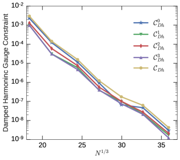
Figure 1: Convergence test for solving the elliptic equations (Eq. (20)) to construct a single BH in the damped harmonic gauge. Plotted are the damped harmonic constraints (cf. Eqs. (32) and (33)) as a function of the number of collocation points per dimension in the domain. As expected for spectral methods, the constraints converge exponentially.

Figure 1 shows the values of the damped harmonic constraints as a function of numerical resolution, where higher resolution is achieved by setting a lower AMR error tolerance. We note that the constraints decrease exponentially with resolution, as expected for a spectral method.

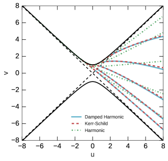
Figure 2: Kruskal-Szekeres diagram showing constant time slices of the unique horizon-penetrating time-independent slicings of Schwarzschild spacetime in damped harmonic and harmonic coordinates, and constant time slices in Kerr-Schild coordinates. The solid black curves represent the curvature singularity while the dashed black lines represent the event horizon. Note that the damped harmonic slices only extend up to the event horizon because we restrict our numerical solution to this region; nevertheless, the damped harmonic slices are horizon-penetrating. Interestingly, we see that the damped harmonic slices are quite close to the Kerr-Schild slices.

III.3 Choosing a time slice

The solution of the elliptic equations along with Eq. (13) gives us a transformation from Kerr-Schild coordinates ($x^{\overline{a}}$) to damped harmonic coordinates ($x^{a}$). But the desired initial data requires computing the metric and its derivatives on a slice of constant time in the new coordinates $x^{a}$, so it is necessary to construct such a slice as a function of the Kerr-Schild coordinates. Using Eq. (13), we can construct a $x^{0}=0$ slice as follows:

$$x^{0}=0=T^{0}{}_{\widehat{a}}~{}x^{\widehat{a}},$$ (34)

$$x^{\widehat{0}}=\frac{-T^{0}{}_{\widehat{i}}}{T^{0}{}_{\widehat{0}}}~{}x^{\widehat{i}},$$ (35)

$$x^{i}=T^{i}{}_{\widehat{a}}~{}x^{\widehat{a}}=\frac{-T^{i}{}_{\widehat{0}}~{}T^{0}{}_{\widehat{i}}}{T^{0}{}_{\widehat{0}}}~{}x^{\widehat{i}}+T^{i}{}_{\widehat{i}}~{}x^{\widehat{i}}.$$ (36)

This gives us a constant-time slice of damped harmonic coordinates ($x^{0}=0$, $x^{i}$) in terms of the intermediate coordinates ($x^{\widehat{a}}$), which in turn are expressed as a transformation from Kerr-Schild coordinates (Eqs. (15)).

The final step in constructing single-BH initial data is to compute the metric and its derivatives on a slice of constant $x^{0}=0$. This is done by choosing a set of points in the new coordinates ($x^{0}=0$, $x^{i}$), computing the corresponding $x^{\widehat{a}}$ using Eqs. (35) and (36), computing the corresponding Kerr-Schild coordinates $x^{\overline{a}}$ using Eqs. (15), and evaluating the metric and its derivatives analytically at those values of $x^{\overline{a}}$ using the Kerr-Schild expressions. The components of the metric and its derivatives are then transformed using the Jacobians (and Hessians for the metric derivatives) that relate $x^{\overline{a}}$ and $x^{a}$.

To visualize the embedding of these damped harmonic slices in spacetime, we restrict ourselves to a nonspinning BH with zero boost. In this spherically symmetric case, we can use the Kruskal-Szekeres coordinates to display the time slices on a spacetime diagram. These are shown in Fig 2, along with constant Kerr-Schild time slices and constant time slices of the unique time-independent horizon-penetrating harmonic slicing of Schwarzschild spacetime Cook and Scheel (1997). We note that constant time slices of damped harmonic coordinates lie nearly on top of the constant time slices of Kerr-Schild coordinates, indicating that the extrinsic curvature of the two slicings are quite similar.

Figure 3: Snapshots during the evolution of a single BH with mass $M=1$ and dimensionless spin $\chi_{z}=0.5$, starting in Kerr-Schild coordinates and moving into damped harmonic coordinates over a time scale of $50M$. Certain components of the spatial metric $g_{ij}$, extrinsic curvature $K_{ij}$, shift $N^{i}$ and lapse $N$ along the $x$-axis are shown as dashed red lines as the evolution progresses. The horizontal axis shows the $x$ coordinate. For each column, time flows downwards and is shown in the left most column. The solid blue lines show our solution for a single time-independent BH in damped harmonic gauge, as described in Sec. III. This solution agrees with the final state of the evolution.

IV Validation against single black hole simulations

In this section, we check whether the solution we constructed in Sec. III agrees with the time-independent final state of a single BH that begins in some different gauge and is evolved numerically using damped harmonic gauge conditions.

We start with a single BH on a $t=0$ slice of Kerr-Schild coordinates, and we evolve it using the following time-dependent gauge source function:

$$H^{a}(t)=\widehat{H}^{a}~{}e^{-t^{4}/\sigma^{4}}+H_{DH}^{a}.$$ (37)

Here $\widehat{H}^{a}$ is the equilibrium gauge source function satisfying Eqs. (2) and (3) for a single Kerr black hole in Kerr-Schild coordinates. It is computed analytically as a known function of $t$ and $x^{i}$ during the evolution. $H_{DH}^{a}$ is the damped harmonic gauge source function given by Eq. (6) and Eq. (7), where we set $f_{0}(t)=1-e^{-t^{4}/\sigma^{4}}$. During the evolution, $H_{a}$ is computed numerically using live values of the metric and its derivatives. We choose the time scale of the gauge transformation, $\sigma$, to be $50M$. At early times, the BH remains time-independent in Kerr-Schild coordinates, then there is a transition on a timescale of $50M$ in which the solution is dominated by gauge dynamics, and at late times the solution obeys the damped harmonic gauge condition and settles down to a time-independent state.

Figure 3 shows the evolution of certain components of the metric as the evolution progresses. These are compared against the single BH damped harmonic solution of Sec. III. The final steady state solution of the simulation agrees with our solution for the time-independent single BH in damped harmonic coordinates. We note that the extrinsic curvature, lapse and shift of the initial state, which is a black hole in Kerr-Schild coordinates, are quite close to the corresponding quantities in the final state; these are all quantities that depend on the embedding of the constant time hypersurfaces in spacetime. We have already seen from Fig. 2 that for zero spin, this embedding is very similar for Kerr-Schild and damped harmonic slicings; Fig. 3 suggests that this embedding is also similar for nonzero spin.

V Conclusion

The damped harmonic gauge has been useful for simulations of binary black hole spacetimes, and is a key ingredient for handling mergers in simulations that use the generalized harmonic formalism. However, currently there is no prescription to construct quasi-equilibrium binary black hole initial data in this gauge; until now, there has been no prescription to construct even a time-independent single black hole in this gauge.

In this work we have developed a method to construct a time-independent boosted, spinning single black hole in damped harmonic gauge. We start with a black hole in Kerr-Schild coordinates, and we construct a coordinate transformation to damped harmonic coordinates. This transformation involves the numerical solution of four coupled, nonlinear elliptic equations with appropriate boundary conditions. We solve these equations with a spectral elliptic solver, and we verify that the solution agrees with the final time-independent state of a single black hole that begins in Kerr-Schild coordinates and is evolved using the damped harmonic gauge.

Our procedure to construct a time-independent boosted, spinning, single BH in damped harmonic coordinates can now be used to construct equilibrium BBH initial data that satisfies the damped harmonic gauge. This is done by superposing two time-independent damped-harmonic BH solutions, in the same way that BBH initial data is currently built by superposing two time-independent Kerr-Schild BH solutions.

The next step is to use the solutions here to construct a BBH initial data set in damped harmonic gauge, evolve it, and compare with evolutions of BBH initial data sets in harmonic gauge and in superposed Kerr-Schild coordinates. This is done in a separate work, Ref. Varma et al. (2018).